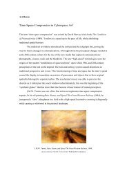
52CHAPTER 4. THE “TRENCH” PROBLEM AND THE PROPOSED SOLUTIONS (a) (b) (c) (d) Figure 4.11: A Lena image with Salt&Pepper noise cleaned with an adaptive SE filter using filtering depth 3. Maximal size of structuring element here is 2 × 2. Notice that there are still part of the noise pixels. (a) Original <strong>Image</strong> (b) <strong>Image</strong> corrupted by the noise (c) erosion of Noisy <strong>Image</strong> (d) opening of Noisy <strong>Image</strong>
4.2. FILTERING USING MULTIPLE MINIMAL PATHS 53 4.2 Filtering using multiple minimal paths An alternative way to avoid the trenches is to store, for each flat zone, all possible combinations of the path-variations, and to choose the most suitable one during filtering. The suitable path-variation is one that has a maximal common-part length. For the example given in Table 2.1, we can store, for the skeleton point x = 5, both BTV transform possibilities {−2, 13, −1} and {8, −3, 5}. Graphically, it can be seen in Fig. 4.6 that the vertex 5, (x = 5), has 2 possible origins - one from the vertex 4 and another from vertex 6. For x = 4, the alternating sequence is {−2, 13}, thus its father is vertex 3. Therefore, the infimum path-variation of the two neighbors x = 4 and x = 5 is either {0} or {−2, 13}, depending on which option we will choose. We choose the path-variation that has a maximal common part length - the option where vertex 4 is the father of vertex 5, that is, {−2, 13}. Of course, this process is more complex and more memory consuming. Another possible implementation is to store the information about multiple pos- sibilities for minimal paths, by enabling connections of the nodes to the multiple fathers in the TD-Tree. This saves the memory usage, but the price is computational overhead. In this case, the path-variation will be created a number of times for each pixel during the filtering, instead of to create it once for each flat zone - before the filtering. Our implementation uses the first option of storing multiple paths for each vertex. A drawback of this approach is that it does not fit all cases, but only those where the topographic distance is equal in the different paths. Obviously, it ignores a large number of cases, because the topographic distance does not have to be equal for multiple paths. Therefore, some trenches remain after the filtering. See the example given in Fig. 4.12. This method has another significant drawback - the performance issue. For real- world images, the number of combinations become very large, and the computation time and memory requirements are exponentially dependent on the number of flat zones in the image. Probably, it is possible, by using some heuristic methods, to reduce significantly the computation requirements, but this issue is out of the scope of this thesis.