Thesis (PDF) - Signal & Image Processing Lab

76 CHAPTER 6. EXTREMA-WATERSHED TREE EXAMPLE
The selected tree-representation was designed with the purpose of achieving good
properties for tasks such as denoising and segmentation. The resulting tree-representation
is called Extrema-Watershed Tree (EWT), and it yields a new set of morphological
operators, derived from the Extrema Watershed Tree, by the general framework of
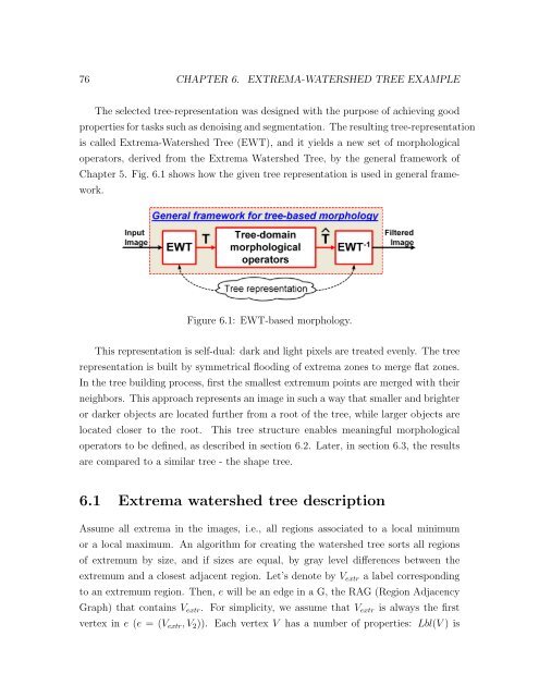
Chapter 5. Fig. 6.1 shows how the given tree representation is used in general frame-
work.
Figure 6.1: EWT-based morphology.
This representation is self-dual: dark and light pixels are treated evenly. The tree
representation is built by symmetrical flooding of extrema zones to merge flat zones.
In the tree building process, first the smallest extremum points are merged with their
neighbors. This approach represents an image in such a way that smaller and brighter
or darker objects are located further from a root of the tree, while larger objects are
located closer to the root. This tree structure enables meaningful morphological
operators to be defined, as described in section 6.2. Later, in section 6.3, the results
are compared to a similar tree - the shape tree.
6.1 Extrema watershed tree description
Assume all extrema in the images, i.e., all regions associated to a local minimum
or a local maximum. An algorithm for creating the watershed tree sorts all regions
of extremum by size, and if sizes are equal, by gray level differences between the
extremum and a closest adjacent region. Let’s denote by Vextr a label corresponding
to an extremum region. Then, e will be an edge in a G, the RAG (Region Adjacency
Graph) that contains Vextr. For simplicity, we assume that Vextr is always the first
vertex in e (e = (Vextr, V2)). Each vertex V has a number of properties: Lbl(V ) is