Master's Thesis in Theoretical Physics - Universiteit Utrecht

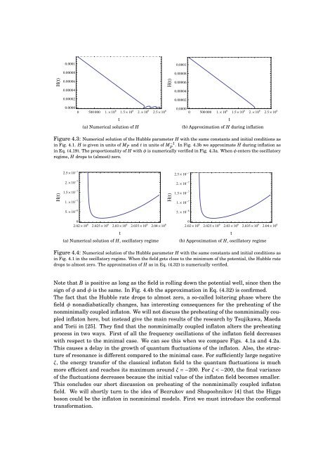
0.00010.00010.000080.00008Ht0.00006Ht0.000060.000040.000040.000020.000020.00000 500 000 1. 10 6 1.5 10 6 2. 10 6 2.5 10 6(a) Numerical solution of Ht0.00000 500 000 1. 10 6 1.5 10 6 2. 10 6 2.5 10 6t(b) Approximation of H during inflationFigure 4.3: Numerical solution of the Hubble parameter H with the same constants and initial conditions asin Fig. 4.1. H is given in units of M P and t in units of M −1 . In Fig. 4.3b we approximate H during inflation asPin Eq. (4.19). The proportionality of H with φ is numerically verified in Fig. 4.3a. When φ enters the oscillatoryregime, H drops to (almost) zero.2.5 10 7 t2.5 10 7 tHt2. 10 71.5 10 71. 10 75. 10 8Ht2. 10 71.5 10 71. 10 75. 10 802.02 10 6 2.025 10 6 2.03 10 6 2.035 10 6 2.04 10 602.02 10 6 2.025 10 6 2.03 10 6 2.035 10 6 2.04 10 6(a) Numerical solution of H, oscillatory regime(b) Approximation of H, oscillatory regimeFigure 4.4: Numerical solution of the Hubble parameter H with the same constants and initial conditions asin Fig. 4.1 in the oscillatory regime. When the field gets close to the minimum of the potential, the Hubble ratedrops to almost zero. The approximation of H as in Eq. (4.32) is numerically verified.Note that B is positive as long as the field is rolling down the potential well, since then thesign of φ and ˙φ is the same. In Fig. 4.4b the approximation in Eq. (4.32) is confirmed.The fact that the Hubble rate drops to almost zero, a so-called loitering phase where thefield φ nonadiabatically changes, has interesting consequences for the preheating of thenonminimally coupled inflaton. We will not discuss the preheating of the nonminimally coupledinflaton here, but instead give the main results of the research by Tsujikawa, Maedaand Torii in [25]. They find that the nonminimally coupled inflaton alters the preheatingprocess in two ways. First of all the frequency oscillations of the inflaton field decreaseswith respect to the minimal case. We can see this when we compare Figs. 4.1a and 4.2a.This causes a delay in the growth of quantum fluctuations of the inflaton. Also, the structureof resonance is different compared to the minimal case. For sufficiently large negativeξ, the energy transfer of the classical inflaton field to the quantum fluctuations is muchmore efficient and reaches its maximum around ξ = −200. For ξ < −200, the final varianceof the fluctuations decreases because the initial value of the inflaton field becomes smaller.This concludes our short discussion on preheating of the nonminimally coupled inflatonfield. We will shortly turn to the idea of Bezrukov and Shaposhnikov [4] that the Higgsboson could be the inflaton in nonminimal models. First we must introduce the conformaltransformation.