Calvo vs. Rotemberg in a Trend Inflation World - Wiwi Uni-Frankfurt
Calvo vs. Rotemberg in a Trend Inflation World - Wiwi Uni-Frankfurt
Calvo vs. Rotemberg in a Trend Inflation World - Wiwi Uni-Frankfurt
Create successful ePaper yourself
Turn your PDF publications into a flip-book with our unique Google optimized e-Paper software.
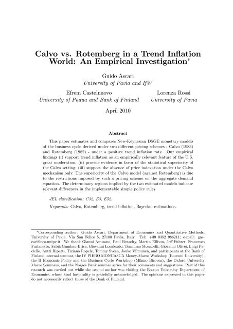
<strong>Calvo</strong> <strong>vs</strong>. <strong>Rotemberg</strong> <strong>in</strong> a <strong>Trend</strong> In‡ation<br />
<strong>World</strong>: An Empirical Investigation<br />
Guido Ascari<br />
<strong>Uni</strong>versity of Pavia and IfW<br />
Efrem Castelnuovo<br />
<strong>Uni</strong>versity of Padua and Bank of F<strong>in</strong>land<br />
April 2010<br />
Abstract<br />
Lorenza Rossi<br />
<strong>Uni</strong>versity of Pavia<br />
This paper estimates and compares New-Keynesian DSGE monetary models<br />
of the bus<strong>in</strong>ess cycle derived under two di¤erent pric<strong>in</strong>g schemes - <strong>Calvo</strong> (1983)<br />
and <strong>Rotemberg</strong> (1982) - under a positive trend <strong>in</strong>‡ation rate. Our empirical<br />
…nd<strong>in</strong>gs (i) support trend <strong>in</strong>‡ation as an empirically relevant feature of the U.S.<br />
great moderation; (ii) provide evidence <strong>in</strong> favor of the statistical superiority of<br />
the <strong>Calvo</strong> sett<strong>in</strong>g; (iii) support the absence of price <strong>in</strong>dexation under the <strong>Calvo</strong><br />
mechanism only. The superiority of the <strong>Calvo</strong> model (aga<strong>in</strong>st <strong>Rotemberg</strong>) is due<br />
to the restrictions imposed by such a pric<strong>in</strong>g scheme on the aggregate demand<br />
equation. The determ<strong>in</strong>acy regions implied by the two estimated models <strong>in</strong>dicate<br />
relevant di¤erences <strong>in</strong> the implementable simple policy rules.<br />
JEL classi…cation: C32, E3, E52.<br />
Keywords: <strong>Calvo</strong>, <strong>Rotemberg</strong>, trend <strong>in</strong>‡ation, Bayesian estimations.<br />
Correspond<strong>in</strong>g author: Guido Ascari, Department of Economics and Quantitative Methods,<br />
<strong>Uni</strong>versity of Pavia, Via San Felice 5, 27100 Pavia, Italy. Tel: +39 0382 986211; e-mail: gascari@eco.unipv.it.<br />
We thank Gianni Amisano, Paul Beaudry, Mart<strong>in</strong> Ellison, Je¤ Fuhrer, Francesco<br />
Furlanetto, Fabià Gumbau-Brisa, Giovanni Lombardo, Tommaso Monacelli, Giovanni Olivei, Luigi Paciello,<br />
Antti Ripatti, Tiziano Ropele, Tommy Sveen, Jouko Vilmunen, and participants at the Bank of<br />
F<strong>in</strong>land <strong>in</strong>ternal sem<strong>in</strong>ar, the IV PIERO MONCASCA Money-Macro Workshop (Bocconi <strong>Uni</strong>versity),<br />
the II Economic Policy and the Bus<strong>in</strong>ess Cycle Workshop (Milano Bicocca), the Oxford <strong>Uni</strong>versity<br />
Macro Sem<strong>in</strong>ars, and the Norges Bank sem<strong>in</strong>ar series for their comments and suggestions. Part of this<br />
research was carried out while the second author was visit<strong>in</strong>g the Boston <strong>Uni</strong>versity Department of<br />
Economics, whose k<strong>in</strong>d hospitality is gratefully acknowledged. The op<strong>in</strong>ions expressed <strong>in</strong> this paper<br />
do not necessarily re‡ect those of the Bank of F<strong>in</strong>land.
1 Introduction<br />
The <strong>Calvo</strong> (1983) and <strong>Rotemberg</strong> (1982) models are the two most popular pric<strong>in</strong>g<br />
schemes <strong>in</strong> the New-Keynesian bus<strong>in</strong>ess cycle literature. 1 Under the typically employed<br />
l<strong>in</strong>ear approximation around "zero <strong>in</strong>‡ation <strong>in</strong> steady state", these two pric<strong>in</strong>g mecha-<br />
nisms lead to the very same reduced-form macroeconomic dynamics (<strong>Rotemberg</strong>, 1987,<br />
Roberts, 1995) and to equivalent welfare <strong>in</strong>dications (Nisticò, 2007). 2 Given such a<br />
model equivalence, the choice of the <strong>Calvo</strong> <strong>vs</strong>. <strong>Rotemberg</strong> pric<strong>in</strong>g scheme has typically<br />
been no more than a matter of macroeconomists’taste.<br />
In a recent contribution, Ascari and Rossi (2009) show that, contrary to conventional<br />
wisdom, the <strong>Calvo</strong> and <strong>Rotemberg</strong> models may imply substantially di¤erent macroeco-<br />
nomic dynamics if log-l<strong>in</strong>earized around a positive steady state <strong>in</strong>‡ation rate, that is<br />
assum<strong>in</strong>g trend <strong>in</strong>‡ation. 3 The two models, then, have very di¤erent policy implica-<br />
tions regard<strong>in</strong>g the <strong>in</strong>‡ation-output relationships, the determ<strong>in</strong>acy conditions, and the<br />
dis<strong>in</strong>‡ation dynamics. 4 Given that (i) the <strong>Calvo</strong> and the <strong>Rotemberg</strong> models are the<br />
two most popular way of modell<strong>in</strong>g nom<strong>in</strong>al price rigidities, (ii) they result <strong>in</strong> di¤er-<br />
ent log-l<strong>in</strong>earized dynamic macroeconomic models under positive trend <strong>in</strong>‡ation, and<br />
that (iii) positive mean <strong>in</strong>‡ation is an undeniable empirical fact <strong>in</strong> OECD countries<br />
<strong>in</strong> the post-WWII sample, it seems natural to proceed to a comparative quantitative<br />
<strong>in</strong>vestigation of these two pric<strong>in</strong>g schemes.<br />
This paper …ts the <strong>Calvo</strong> and <strong>Rotemberg</strong> frameworks derived under positive trend<br />
1For <strong>in</strong>-depth analyses of the new-Keynesian model of the bus<strong>in</strong>ess cycle, see K<strong>in</strong>g (2000) and<br />
Woodford (2003).<br />
2Lombardo and Vest<strong>in</strong> (2008) discuss the conditions under which welfare costs might be di¤erent<br />
under these two pric<strong>in</strong>g schemes.<br />
3As <strong>in</strong> the literature, trend <strong>in</strong>‡ation <strong>in</strong>dicates a positive steady state level of <strong>in</strong>‡ation.<br />
4The zero steady state assumption, which is empirically problematic, has already been questioned<br />
from a theoretical standpo<strong>in</strong>t. Ascari (2004) and Yun (2005) show that …rst-order e¤ects arise on the<br />
<strong>Calvo</strong> price sett<strong>in</strong>g setup under trend <strong>in</strong>‡ation. Elaborat<strong>in</strong>g further with the <strong>Calvo</strong> set-up, Ascari and<br />
Ropele (2007, 2009) study the implications of di¤erent trend <strong>in</strong>‡ation levels for the optimal monetary<br />
policy and for the Taylor pr<strong>in</strong>ciple.<br />
2
<strong>in</strong>‡ation to 1984:I-2008:II U.S. macroeconomic data. Several …nd<strong>in</strong>gs arise. First,<br />
models acknowledg<strong>in</strong>g a positive trend <strong>in</strong>‡ation rate display a better (or, at least,<br />
no worse) …t than a basel<strong>in</strong>e "zero <strong>in</strong>‡ation <strong>in</strong> steady state" framework. Given the<br />
di¤erent policy implications stemm<strong>in</strong>g from a trend <strong>in</strong>‡ation-equipped framework (as<br />
opposed to the basel<strong>in</strong>e model) <strong>in</strong> terms of optimal policy and determ<strong>in</strong>acy of simple<br />
monetary policy rules (Ascari and Ropele, 2007, 2009), our results push towards the<br />
employment and development of macroeconomic frameworks consistently account<strong>in</strong>g for<br />
a positive steady-state <strong>in</strong>‡ation rate. Second, the U.S. data support <strong>Calvo</strong> (as opposed<br />
to <strong>Rotemberg</strong>) as the better …tt<strong>in</strong>g pric<strong>in</strong>g scheme. In particular, when compar<strong>in</strong>g<br />
the two models under the "no price-<strong>in</strong>dexation" restriction, we verify the rejection of<br />
the <strong>in</strong>dexation hypothesis by the <strong>Calvo</strong> framework. Interest<strong>in</strong>gly, this result emerges<br />
<strong>in</strong> absence of any stochastic model for the low frequency of the <strong>in</strong>‡ation rate, i.e.<br />
without appeal<strong>in</strong>g to any exogenous process model<strong>in</strong>g the possibly time-vary<strong>in</strong>g trend<br />
<strong>in</strong>‡ation as <strong>in</strong> Ireland (2007) and Cogley and Sbordone (2008). Di¤erently, shutt<strong>in</strong>g<br />
down <strong>in</strong>dexation <strong>in</strong> the <strong>Rotemberg</strong> framework leads to a drop <strong>in</strong> the model’s empirical<br />
…t, suggest<strong>in</strong>g a lack of <strong>in</strong>ternal dynamics <strong>in</strong> comparison to <strong>Calvo</strong>. Third, conditional<br />
on estimated (as opposed to calibrated) frameworks, the determ<strong>in</strong>acy area is shown<br />
to be strongly dependent on the choice of the price sett<strong>in</strong>g model. In particular, the<br />
set of implementable simple rules conditional on our estimated New-Keynesian model<br />
under positive trend <strong>in</strong>‡ation and <strong>Calvo</strong> price sett<strong>in</strong>g is substantially smaller than<br />
the one associated to the New-Keynesian framework derived under the standard zero<br />
steady-state assumption, and even smaller than that implied by the widely employed<br />
<strong>Rotemberg</strong> framework. Our empirical results po<strong>in</strong>ts toward the <strong>Calvo</strong> mechanism as<br />
the better …tt<strong>in</strong>g pric<strong>in</strong>g scheme. Thus, from a policy standpo<strong>in</strong>t, they suggest that<br />
policymakers should refra<strong>in</strong> from loosen<strong>in</strong>g monetary policy and stay hawkish, i.e., they<br />
should keep react<strong>in</strong>g strongly to the evolutions of the <strong>in</strong>‡ation rate.<br />
3
Other papers stress the importance of consider<strong>in</strong>g trend <strong>in</strong>‡ation <strong>in</strong> empirical work.<br />
Benati (2008) estimates a NKPC for a variety of countries, and shows that price-<br />
<strong>in</strong>dexation à la Christiano, Eichenbaum, and Evans (2005) is not stable across di¤erent<br />
samples <strong>in</strong> countries that explicitly adopted an <strong>in</strong>‡ation target<strong>in</strong>g scheme. He relates<br />
this <strong>in</strong>stability to di¤erent policy regimes, so demonstrat<strong>in</strong>g that <strong>in</strong>dexation is "not<br />
structural <strong>in</strong> the sense of Lucas". Elaborat<strong>in</strong>g on this paper, Benati (2009) estimates<br />
di¤erent NKPCs derived under alternative pric<strong>in</strong>g schemes. His results corroborate and<br />
extend his previous …nd<strong>in</strong>gs, i.e. the degree of price <strong>in</strong>dexation is not <strong>in</strong>variant across<br />
di¤erent policy regimes, and it tends to zero under the more recent, stable regimes.<br />
Notably, Benati (2009) supports, among others, Ascari and Ropele’s (2009) derivation<br />
of the <strong>Calvo</strong> model under trend <strong>in</strong>‡ation for a variety of countries. 5 He considers a<br />
step-function to model possible drifts <strong>in</strong> the <strong>in</strong>‡ation target. Di¤erently from Benati<br />
(2009), who works with a fully-‡edged New-Keynesian DSGE framework, Cogley and<br />
Sbordone (2008) estimate a NKPC embedd<strong>in</strong>g a drift<strong>in</strong>g trend <strong>in</strong>‡ation coupled with<br />
a TVC-VAR model. They …nd that, once drifts <strong>in</strong> trend <strong>in</strong>‡ation are accounted for,<br />
price <strong>in</strong>dexation <strong>in</strong> the U.S. is zero, i.e. a purely-forward look<strong>in</strong>g NKPC …ts the data<br />
well without the need for ad-hoc backward-look<strong>in</strong>g components. 6 Coibion and Gorod-<br />
nichenko (2009) estimate a Taylor rule with trend <strong>in</strong>‡ation for the post-WWII, and<br />
couple it with a calibrated New-Keynesian model derived under positive trend <strong>in</strong>‡a-<br />
tion. They show that the U.S. economy switched to determ<strong>in</strong>acy dur<strong>in</strong>g the Volcker<br />
dis<strong>in</strong>‡ation because of changes <strong>in</strong> the Federal Reserve’s response to macro variables and<br />
the decl<strong>in</strong>e <strong>in</strong> trend <strong>in</strong>‡ation. 7 Paciello (2009) estimates a <strong>Calvo</strong>-based NKPC with<br />
5 The list considered by Benati (2009) <strong>in</strong>cludes the Euro area, West Germany, Germany, France,<br />
Italy, U.K., Canada, Sweden, Australia, New Zealand, and Switzerland.<br />
6 Barnes, Gumbau-Brisa, Lie, and Olivei (2009) use a di¤erent estimation methodology and a more<br />
‡exible <strong>in</strong>dexation-scheme with respect to Cogley and Sbordone (2008), and show that <strong>in</strong>dexation to<br />
past <strong>in</strong>‡ation may be substantial <strong>in</strong> the post-WWII sample.<br />
7 Schorfheide (2005) and Ireland (2007) also embed a time-vary<strong>in</strong>g <strong>in</strong>‡ation target <strong>in</strong> their models,<br />
but without consequences for the speci…cation of the NKPC due to the assumption of full-<strong>in</strong>dexation.<br />
4
constant trend <strong>in</strong>‡ation for the post-WWII via <strong>in</strong>direct <strong>in</strong>ference, and shows that such<br />
a model is able to match the dynamic responses of <strong>in</strong>‡ation to monetary policy and<br />
technology shocks even <strong>in</strong> absence of <strong>in</strong>dexation, an ability not enjoyed by the standard,<br />
zero steady-state <strong>in</strong>‡ation framework.<br />
Our <strong>in</strong>vestigation departs from the ones above along di¤erent dimensions. First<br />
and foremost, our paper focuses on the estimation of, and the empirical comparison<br />
between, two di¤erent frameworks, i.e. <strong>Calvo</strong> and <strong>Rotemberg</strong>. To our knowledge, this<br />
is the only contribution to date assess<strong>in</strong>g the relative empirical relevance of these two<br />
very widely employed pric<strong>in</strong>g schemes under trend <strong>in</strong>‡ation. Second, we focus on two<br />
models display<strong>in</strong>g a constant trend <strong>in</strong>‡ation rate, i.e. display<strong>in</strong>g no exogenous random-<br />
walk type of process for the Fed’s <strong>in</strong>‡ation target. Still, the version of the <strong>Calvo</strong> model<br />
preferred by the data is that with no-price <strong>in</strong>dexation. With respect to Benati (2009),<br />
we provide evidence for the U.S. case, therefore complement<strong>in</strong>g his battery of estimates.<br />
With respect to Cogley and Sbordone (2008) and Paciello (2009), we consider a struc-<br />
tural representation of the demand side of the economy, rather than a reduced-form<br />
TVC-VAR. This is obviously important from an econometric standpo<strong>in</strong>t, because the<br />
identi…cation of forward and backward look<strong>in</strong>g terms <strong>in</strong> the NKPC also depends on how<br />
the rema<strong>in</strong><strong>in</strong>g structural equations are modeled. When such equations are not speci…ed,<br />
as <strong>in</strong> the NKPC-VAR approach, the mean<strong>in</strong>g of the economic restrictions imposed to<br />
the estimation is unclear, as po<strong>in</strong>ted out by Cogley and Sbordone (2008) themselves.<br />
Also from a theoretical po<strong>in</strong>t of view, our analysis shows the importance of estimat<strong>in</strong>g<br />
the full model equations, because the assumed pric<strong>in</strong>g scheme may a¤ect not only the<br />
supply side of the model, but also the other model equations, as <strong>in</strong> the case of the<br />
<strong>Rotemberg</strong> model. Moreover, di¤erently from Paciello (2009), we conduct our empir-<br />
ical analysis with Bayesian techniques. Our choice is driven by the possibly superior<br />
performance aga<strong>in</strong>st <strong>in</strong>direct <strong>in</strong>ference (impulse response match<strong>in</strong>g) as far as this class<br />
5
of DSGE models is concerned (Canova and Sala, 2009). F<strong>in</strong>ally, we concentrate on a<br />
stable subsample (great moderation), which is likely to feature a unique equilibrium<br />
even under historically plausible values for trend <strong>in</strong>‡ation (Coibon and Gorodnichenko,<br />
2009), and a more stable low-frequency component of <strong>in</strong>‡ation. This sample choice<br />
makes our assumption of a constant trend <strong>in</strong>‡ation more palatable. Moreover, it does<br />
not <strong>in</strong>corporate the real output losses caused by the "imperfect credibility" of the Vol-<br />
cker dis<strong>in</strong>‡ation (Goodfriend and K<strong>in</strong>g, 2005), which is not modeled <strong>in</strong> this paper. We<br />
see our contribution as complementary to those presented above.<br />
The paper is structured as follows. Section 2 describes the two frameworks we<br />
deal with and highlights the relevant di¤erences. Section 3 presents and discusses our<br />
empirical …nd<strong>in</strong>gs, with particular emphasis on the estimated degree of price <strong>in</strong>dexation.<br />
Section 4 compares the prescriptions of our estimated models <strong>in</strong> terms of implementable<br />
simple policy rules. Section 5 scrut<strong>in</strong>izes further the two pric<strong>in</strong>g schemes, and discusses<br />
the reasons of <strong>Calvo</strong>’s superiority. Section 6 concludes, and draws some directions for<br />
further research.<br />
2 The theoretical models<br />
In this section we sketch a small-scale New-Keynesian model <strong>in</strong> the two versions of<br />
the <strong>Rotemberg</strong> (1982) and the <strong>Calvo</strong> (1983) price sett<strong>in</strong>g scheme. The model econ-<br />
omy is composed of a cont<strong>in</strong>uum of <strong>in</strong>…nitely-lived consumers, producers of …nal and<br />
<strong>in</strong>termediate goods. Households have the follow<strong>in</strong>g <strong>in</strong>stantaneous and separable utility<br />
function:<br />
U (Ct; Nt) = C1<br />
t+j<br />
1<br />
N<br />
dn<br />
1+'<br />
t+j<br />
1 + ' ;<br />
where Ct is a consumption basket (with elasticity of substitution among goods ") and<br />
Nt are labor hours.<br />
F<strong>in</strong>al good market is competitive and the production function is given by Yt =<br />
6
h R 1<br />
0<br />
" 1<br />
" Y i;t di<br />
i "<br />
" 1<br />
to Yi;t+j = Pi;t<br />
Pt+j<br />
: F<strong>in</strong>al good producers demand for <strong>in</strong>termediate <strong>in</strong>puts is therefore equal<br />
"<br />
Yt+j. The <strong>in</strong>termediate <strong>in</strong>puts Yi;t are produced by a cont<strong>in</strong>uum of<br />
…rms <strong>in</strong>dexed by i 2 [0; 1] with the follow<strong>in</strong>g simple constant return to scale technology<br />
Yi;t = AtNi;t; where labor is the only <strong>in</strong>put and ln At = at is an exogenous productivity<br />
shock, which follows an AR(1) process. The <strong>in</strong>termediate good sector is monopolistically<br />
competitive.<br />
2.1 Firms and Price Sett<strong>in</strong>g: <strong>Rotemberg</strong> (1982) <strong>vs</strong>. <strong>Calvo</strong><br />
(1983)<br />
The <strong>Calvo</strong> model<br />
The <strong>Calvo</strong> price sett<strong>in</strong>g scheme assumes that <strong>in</strong> each period there is a …xed probability<br />
1 that a …rm can re-optimize its nom<strong>in</strong>al price, i.e., P i;t: With probability , <strong>in</strong>stead,<br />
the …rm automatically and costlessy adjust its price accord<strong>in</strong>g to an <strong>in</strong>dexation rule.<br />
The price sett<strong>in</strong>g problem is:<br />
max<br />
P i;t<br />
where Dt;t+j<br />
Et<br />
1X<br />
j=0<br />
s.t. Yi;t+j =<br />
t;t+j 1 =<br />
Dt;t+j j<br />
" Pi;t ( j ) 1<br />
( Pt<br />
" Pi;t ( j ) 1<br />
Pt 1<br />
Pt+j<br />
Pt+1<br />
Pt<br />
Pt+j<br />
t;t+j 1<br />
t;t+j 1<br />
# "<br />
Yi;t+j MC r i;t+jYi;t+j<br />
#<br />
, (1)<br />
Yt+j and (2)<br />
Pt+j 1<br />
P t+j 2<br />
for j = 1; 2;<br />
1 for j = 0.<br />
j Yt<br />
Yt+j represents …rms’stochastic discount factor, MCr i;t+j = Wi;t+j<br />
Pt+jAt+j is<br />
the real marg<strong>in</strong>al cost function, and denotes the central bank’s <strong>in</strong>‡ation target and it<br />
is equal to the level of trend <strong>in</strong>‡ation. The <strong>in</strong>dexation scheme <strong>in</strong> (1) is very general. In<br />
particular: (i) 2 [0; 1] allows for any degree of price <strong>in</strong>dexation; (ii) 2 [0; 1] allows for<br />
any degree of (geometric) comb<strong>in</strong>ation of the two types of <strong>in</strong>dexation usually employed<br />
<strong>in</strong> the literature: to steady state <strong>in</strong>‡ation (e.g., Yun, 1996) and to past <strong>in</strong>‡ation rates<br />
7<br />
(3)
(e.g., Christiano et al., 2005).<br />
In the <strong>Calvo</strong> price sett<strong>in</strong>g framework, prices are staggered because …rms charg<strong>in</strong>g<br />
prices at di¤erent periods will set di¤erent prices. Then, <strong>in</strong> each given period t, there<br />
will be a distribution of di¤erent prices. Price dispersion results <strong>in</strong> an <strong>in</strong>e¢ ciency loss<br />
<strong>in</strong> aggregate production. Formally:<br />
N d t = Yt<br />
Z 1<br />
At 0<br />
"<br />
Pi;t<br />
di<br />
Pt<br />
| {z }<br />
st<br />
Yt<br />
= st<br />
At<br />
. (4)<br />
Schmitt-Grohé and Uribe (2007) show that st is bounded below at one, so that st<br />
represents the resource costs due to relative price dispersion under the <strong>Calvo</strong> mechanism.<br />
Indeed, the higher st, the more labor N d t is needed to produce a given level of output.<br />
Note that price dispersion creates a wedge between aggregate output and aggregate<br />
employment. To close the model, the aggregate resource constra<strong>in</strong>t is simply given by:<br />
The <strong>Rotemberg</strong> model<br />
Yt = Ct: (5)<br />
The <strong>Rotemberg</strong> model assumes that a monopolistic …rm faces a quadratic cost of<br />
adjust<strong>in</strong>g nom<strong>in</strong>al prices, that can be measured <strong>in</strong> terms of the …nal-good and given by:<br />
' p<br />
2<br />
Pi;t<br />
t 1 ( ) 1 Pi;t 1<br />
1<br />
! 2<br />
Yt; (6)<br />
where ' p > 0 determ<strong>in</strong>es the degree of nom<strong>in</strong>al price rigidity. As stressed <strong>in</strong> <strong>Rotemberg</strong><br />
(1982), the adjustment cost seeks to account for the negative e¤ects of price changes<br />
on the customer-…rm relationship. These negative e¤ects <strong>in</strong>crease <strong>in</strong> magnitude with<br />
the size of the price change and with the overall scale of economic activity, Yt. As<br />
for the <strong>Calvo</strong> model, (6) <strong>in</strong>cludes a general speci…cation for the adjustment cost used<br />
by, e.g., Ireland (2007), among others. In particular, the adjustment cost will depend<br />
on the ratio between the new reset price and the one set dur<strong>in</strong>g the previous period,<br />
8
adjusted by a (geometric) comb<strong>in</strong>ation of steady state <strong>in</strong>‡ation and of past <strong>in</strong>‡ation.<br />
The parameters and play a parallel role as <strong>in</strong> the <strong>in</strong>dexation scheme <strong>in</strong> the <strong>Calvo</strong><br />
model.<br />
The problem for the …rm i is then:<br />
8<br />
1X <<br />
max<br />
fPi;tg1 Et<br />
t=0<br />
j=0<br />
Dt;t+j<br />
:<br />
Pi;t+j<br />
Yi;t+j MC<br />
Pt+j<br />
r i;t+jYi;t+j<br />
s.t. Yi;t+j = Pi;t+j<br />
Pt+j<br />
' p<br />
2<br />
Pi;t+j<br />
t+j 1 ( ) 1 Pi;t+j 1<br />
1<br />
(7)<br />
"<br />
Yt+j; (8)<br />
where the notation is as above. Firms can change their price <strong>in</strong> each period, subject<br />
to the payment of the adjustment cost. Therefore, all the …rms face the same problem,<br />
and thus will choose the same price and output. In other words the equilibrium is<br />
symmetric: Pi;t = Pt; Yi;t = Yt; Wi;t = Wt and MC r i;t = MC r t 8i: Given this symmetry,<br />
and di¤erently with respect to the <strong>Calvo</strong> model, <strong>in</strong> the <strong>Rotemberg</strong> model the aggregate<br />
production function features no <strong>in</strong>e¢ ciency due to price dispersion, therefore:<br />
Yt = AtNt: (9)<br />
In the <strong>Rotemberg</strong> model, the adjustment cost enters the aggregate resource con-<br />
stra<strong>in</strong>t, which creates an <strong>in</strong>e¢ ciency wedge between output and consumption:<br />
Yt =<br />
2<br />
41<br />
' p<br />
2<br />
Pt<br />
t 1 ( ) 1 Pt 1<br />
1<br />
! 2 3<br />
5<br />
1<br />
Ct = t Ct: (10)<br />
Some key-di¤erences between the <strong>Calvo</strong> and the <strong>Rotemberg</strong> model arise. In the <strong>Calvo</strong><br />
model, the cost of nom<strong>in</strong>al rigidities, i.e., price dispersion, creates a wedge between<br />
aggregate employment and aggregate output, mak<strong>in</strong>g aggregate production less e¢ cient.<br />
In the <strong>Rotemberg</strong> model, <strong>in</strong>stead, the cost of nom<strong>in</strong>al rigidities, i.e., the adjustment cost,<br />
creates a wedge between aggregate consumption and aggregate output, because part of<br />
the output goes <strong>in</strong> the price adjustment cost. As shown <strong>in</strong> Ascari and Rossi (2009), and<br />
9<br />
! 2<br />
Yt+j<br />
9<br />
=<br />
; ;
evident from (4) and (10), both these wedges are non-l<strong>in</strong>ear functions of <strong>in</strong>‡ation and<br />
they <strong>in</strong>crease with trend <strong>in</strong>‡ation. However, both wedges take the same unitary value<br />
under two particular cases: (i) a net steady state <strong>in</strong>‡ation equals zero, and/or (ii) full<br />
<strong>in</strong>dexation to past or trend <strong>in</strong>‡ation.<br />
2.2 The log-l<strong>in</strong>earized frameworks<br />
We now present the log-l<strong>in</strong>earized versions of the two pric<strong>in</strong>g frameworks we deal with<br />
(for a full derivation, see Ascari and Ropele, 2007, 2009, and Ascari and Rossi, 2009).<br />
Aga<strong>in</strong>, we stress that the derivation allows for a non-zero value for the <strong>in</strong>‡ation rate <strong>in</strong><br />
steady state, which may be <strong>in</strong>terpreted as the target pursued by the Federal Reserve <strong>in</strong><br />
conduct<strong>in</strong>g the U.S. monetary policy.<br />
The <strong>Calvo</strong> model<br />
The <strong>Calvo</strong> model is described by the follow<strong>in</strong>g …rst-order di¤erence equations:<br />
1 "<br />
t = + ( 1) t+1jt + ^yt 'at + '^st + b t+1jt; (11)<br />
h<br />
b (" 1)(1 ) (" 1)(1 )<br />
t = (1 ) 1<br />
^yt +<br />
(" 1) t+1jt + ^ i<br />
t+1jt ; (12)<br />
bst = t + " "(1 ) bst 1; (13)<br />
^yt = y ^yt+1jt + (1 y)^yt 1<br />
1 bit bt+1jt + gt; (14)<br />
where t bt bt 1; ^ stands for the <strong>in</strong>‡ation rate, ^y for detrended output, a is<br />
the technological shock, g is the demand shock. Hatted variables <strong>in</strong>dicate percentage<br />
deviations with respect to steady state values or, <strong>in</strong> case of output, from a trend. The<br />
notation xt+1jt <strong>in</strong>dicates the expectation <strong>in</strong> t of xt+1: is the relative risk aversion<br />
parameter, ' the labor supply elasticity, the discount factor, " the Dixit-Stiglitz<br />
elasticity of substitution among goods, the <strong>Calvo</strong> parameter, the degree of price<br />
<strong>in</strong>dexation, the relative weight of <strong>in</strong>dexation to past <strong>in</strong>‡ation <strong>vs</strong>. trend <strong>in</strong>‡ation, and<br />
10
the steady-state, trend <strong>in</strong>‡ation rate: F<strong>in</strong>ally, ; ; ; and <strong>in</strong> eqs. (11)-(14) are the<br />
follow<strong>in</strong>g convolutions of parameters:<br />
1 (" 1)(1 ) 1 "(1 )<br />
(" 1)(1 ) ;<br />
1<br />
1 1<br />
(" 1)(1 )<br />
( ;") ( + ') + ( ;") (1 ) ;<br />
" (" 1)(1 ) ( 1 1)<br />
1 (" 1)(1 ) ;<br />
Notably, all the convolutions of the log-l<strong>in</strong>earized model are a function of the trend<br />
<strong>in</strong>‡ation rate ; that generally tends to <strong>in</strong>crease the coe¢ cients on the forward-look<strong>in</strong>g<br />
variables (see Ascari, 2004, Yun, 2005, Hornste<strong>in</strong> and Wolman, 2005 and Kiley, 2007):<br />
Moreover, the log-l<strong>in</strong>earized NKPC is <strong>in</strong>‡uenced by the price dispersion process st.<br />
Under <strong>Calvo</strong>, just a fraction (1 ) of …rms is allowed to reoptimize <strong>in</strong> each period, then<br />
price dispersion arises. Under a strictly positive trend <strong>in</strong>‡ation rate, price dispersion<br />
assumes a …rst-order relevance and <strong>in</strong>‡uences the evolution of the log-l<strong>in</strong>earized <strong>in</strong>‡ation<br />
rate. Moreover, price dispersion has a backward-look<strong>in</strong>g dynamics. The forward look<strong>in</strong>g<br />
auxiliary process t also participates to the determ<strong>in</strong>ation of <strong>in</strong>‡ation.<br />
The aggregate demand equation (14) is expressed <strong>in</strong> hybrid terms à la Fuhrer and<br />
Rudebusch (2004), with the parameter y identify<strong>in</strong>g the relative weight of expected<br />
output. This semi-structural, ‡exible version of the IS curve have successfully been<br />
employed by, among others, Benati (2008, 2009) and Benati and Surico (2008, 2009).<br />
The <strong>Rotemberg</strong> model<br />
The <strong>Rotemberg</strong> model is characterized by the follow<strong>in</strong>g di¤erence equations:<br />
^t = p^t 1 + f ^t+1jt + dy (1 ) ^yt+1jt + mc cmct; (15)<br />
cmct = ( + ') ^yt &c ^t + &c ^t 1 (1 + ')at; (16)<br />
^yt = y ^yt+1jt + (1 y)^yt 1 &c ^t+1jt + &c ^t<br />
11<br />
;<br />
1 ^{t ^t+1jt + gt;(17)
where cmc stands for marg<strong>in</strong>al costs, and the notation has the same <strong>in</strong>terpretation as <strong>in</strong><br />
the previous Subsection. The coe¢ cients p, f, dy, mc, and &c are convolutions of<br />
the structural parameters of the model:<br />
&c = ' p ( 1 1) 1<br />
C<br />
Y<br />
1<br />
= 1<br />
'p 2 ( 1 2 ;<br />
1)<br />
'p ( 1)2<br />
2<br />
% 2 2(1 ) (1 ) (1 + ) C<br />
p =<br />
f =<br />
dy =<br />
Y +<br />
2 2(1 ) (1 ) C<br />
Y + [( 1 1) 1 ] 2 ' p<br />
%<br />
2 2(1 ) (1 ) C<br />
Y + [( 1 1) 1 ] 2 ' p<br />
2(1 ) 1 C<br />
Y<br />
%<br />
mc = " 1 + ' p<br />
;<br />
%<br />
2(1 ) 1 (1 ) C<br />
Y<br />
:<br />
'p% 1<br />
1<br />
1 2 'p (1 + ) ;<br />
As often assumed <strong>in</strong> the literature, 8 it is possible to draw a relationship between<br />
the <strong>Rotemberg</strong> adjustment cost ' p and the <strong>Calvo</strong> parameter impos<strong>in</strong>g the condition<br />
' p =<br />
(" 1)<br />
that implies the same …rst order dynamics of the two models <strong>in</strong> the case<br />
(1 )(1 )<br />
of zero steady state <strong>in</strong>‡ation. Such relationship will enable us to <strong>in</strong>directly estimate the<br />
<strong>Rotemberg</strong> adjustment cost by focus<strong>in</strong>g on the <strong>Calvo</strong> parameter and to use the very<br />
same prior densities for the structural parameters of the two models we ultimately aim<br />
at compar<strong>in</strong>g, i.e. <strong>Calvo</strong> and <strong>Rotemberg</strong>. 9<br />
A few comments are <strong>in</strong> order. First, the impact of trend <strong>in</strong>‡ation is evident when<br />
look<strong>in</strong>g at eqs. (15)-(17) and their convolutions of parameters. As <strong>in</strong> the <strong>Calvo</strong> model,<br />
trend <strong>in</strong>‡ation alters the <strong>in</strong>‡ation dynamics by directly a¤ect<strong>in</strong>g the NKPC coe¢ cients.<br />
Higher trend <strong>in</strong>‡ation <strong>in</strong>creases the coe¢ cient relative to expected and past <strong>in</strong>‡ation<br />
8 See <strong>Rotemberg</strong> (1987) or Lombardo and Vest<strong>in</strong> (2009) for details.<br />
9 We also estimated a version of the <strong>Rotemberg</strong> model <strong>in</strong> which the adjustment cost is a free parameter,<br />
and veri…ed no appreciable variations <strong>in</strong> the marg<strong>in</strong>al likelihood.<br />
12<br />
;
as well as the coe¢ cient of real marg<strong>in</strong>al costs (Ascari and Rossi, 2009). Notice that<br />
the presence of past <strong>in</strong>‡ation <strong>in</strong> (15) is due to <strong>in</strong>dexation to past <strong>in</strong>‡ation. With no<br />
<strong>in</strong>dexation to past <strong>in</strong>‡ation, i.e. with = 0; however, the coe¢ cient p equals zero and<br />
the NKPC becomes completely forward look<strong>in</strong>g. Recall that this is not the case <strong>in</strong> the<br />
<strong>Calvo</strong> model, because even if past <strong>in</strong>‡ation disappears when = 0; price dispersion<br />
dynamics <strong>in</strong>troduces a backward-look<strong>in</strong>g component. Furthermore, the expected di¤er-<br />
ence of detrended output appears <strong>in</strong> the NKPC, eq. (15), because of the <strong>in</strong>‡uence that<br />
trend <strong>in</strong>‡ation exerts over …rms’discount factor.<br />
Second, because of the presence of the price adjustment cost, <strong>in</strong> the <strong>Rotemberg</strong><br />
model the log-l<strong>in</strong>earized resource constra<strong>in</strong>t can be written<br />
^ct = ^yt<br />
'p ( 1 1) 1<br />
'p 1 2 ( 1 1) 2 ^t + 'p ( 1 1) 1<br />
'p 1<br />
2 ( 1 1) 2 ^t 1: (18)<br />
This equation shows that to a …rst order approximation the <strong>Rotemberg</strong> model: (i)<br />
implies a wedge between output and consumption; (ii) this wedge depends positively<br />
on current and past <strong>in</strong>‡ation level; (iii) the coe¢ cients of ^t and ^t 1 <strong>in</strong> (18) <strong>in</strong>crease<br />
with trend <strong>in</strong>‡ation; (iv) the wedge disappears with zero steady state <strong>in</strong>‡ation rate or<br />
with full <strong>in</strong>dexation, i.e. with = 1: Such a wedge a¤ects also the amount of resources<br />
produced <strong>in</strong> the economy. Consequently, the IS, eq. (17), features the …rst di¤erence <strong>in</strong><br />
<strong>in</strong>‡ation rates. The price adjustment cost causes the real marg<strong>in</strong>al cost to depend also<br />
on actual <strong>in</strong>‡ation and past <strong>in</strong>‡ation (see the additional term &c ^t and &c ^t 1 <strong>in</strong><br />
(16)).<br />
Notably, under the peculiar case of zero trend <strong>in</strong>‡ation, i.e., = 1, both the Rotem-<br />
berg and the <strong>Calvo</strong> frameworks l<strong>in</strong>es up with the standard hybrid New-Keynesian for-<br />
mulation allow<strong>in</strong>g for price <strong>in</strong>dexation to past/steady state <strong>in</strong>‡ation. The same holds<br />
true <strong>in</strong> a full <strong>in</strong>dexation scenario, i.e. when = 1.<br />
To sum up, the di¤erent wedges which characterize the <strong>Calvo</strong> and the <strong>Rotemberg</strong><br />
model <strong>in</strong>duce three ma<strong>in</strong> di¤erences <strong>in</strong> the two log-l<strong>in</strong>earized representations. First, the<br />
13
<strong>Calvo</strong> model displays price dispersion, which enters the NKPC as endogenous prede-<br />
term<strong>in</strong>ed variable. By contrast, given the symmetry <strong>in</strong> the <strong>Rotemberg</strong> economy, price<br />
dispersion is absent <strong>in</strong> the <strong>Rotemberg</strong> model. Second, the presence of the price ad-<br />
justment cost <strong>in</strong> the <strong>Rotemberg</strong> model causes the real marg<strong>in</strong>al cost to depend also on<br />
actual and past <strong>in</strong>‡ation. F<strong>in</strong>ally, the price adjustment cost generates a wedge between<br />
output and consumption <strong>in</strong> the resource constra<strong>in</strong>t (10), which is re‡ected <strong>in</strong> the IS<br />
curve (17). As shown by Ascari and Rossi (2009), these di¤erences are relevant from a<br />
policy standpo<strong>in</strong>t, because of their impact on the de…nition of the determ<strong>in</strong>acy territory<br />
associated to simple, implementable Taylor-type rules.<br />
2.3 Clos<strong>in</strong>g the models<br />
The two models are closed by a common set of equations, i.e.<br />
^{t = i^{t 1 + (1 i) ( ^t + y ^yt) + mt; (19)<br />
zt = zzt 1 + "zt; "zt N(0;<br />
2<br />
z); z 2 fa; g; mg : (20)<br />
Eq. (19) is a standard policy rule postulat<strong>in</strong>g a smoothed reaction of the policy<br />
rate ^{t to ‡uctuations <strong>in</strong> <strong>in</strong>‡ation and output, with stochastic deviations driven by the<br />
monetary policy shock mt. Eq. (20) de…nes the stochastic properties of the mutually<br />
uncorrelated shocks hitt<strong>in</strong>g the system.<br />
3 Econometric exercise<br />
Our <strong>in</strong>vestigation focuses on U.S. data. We employ three "observables", i.e. the quar-<br />
terly net growth rate of the GDP de‡ator obs<br />
t , the log-deviation of real GDP with<br />
14
espect to its long run trend y obs<br />
t , 10 and the net Federal Funds Rate obs<br />
t . 11 Our measure<br />
of detrended output, be<strong>in</strong>g ma<strong>in</strong>ly statistical, is robust to model misspeci…cation, and<br />
it is also justi…ed by the absence <strong>in</strong> this model of physical capital, which would proba-<br />
bly return a severely misspeci…ed model-consistent measure of natural output. Output<br />
proxies robust to model misspeci…cation have recently been employed by, among others,<br />
Lubik and Schorfheide (2004), Boiv<strong>in</strong> and Giannoni (2006), Benati (2008, 2009) and<br />
Benati and Surico (2008, 2009). 12<br />
Several authors (Clarida, Galí and Gertler, 2000, Lubik and Schorfeide, 2004, Boiv<strong>in</strong><br />
and Giannoni, 2006, Benati and Surico, 2009, and Mavroeidis, 2009) document a break<br />
<strong>in</strong> the U.S. monetary policy conduct <strong>in</strong> correspondence to the advent of Paul Volcker<br />
as chairman of the Federal Reserve. Changes <strong>in</strong> the U.S. macro-dynamics possibly con-<br />
sequential to such a monetary policy shift have also been <strong>in</strong>vestigated by D’Agost<strong>in</strong>o,<br />
Giannone, and Surico (2006), Benati and Surico (2008) and Cogley, Primiceri, and<br />
Sargent (2009), who document a variation <strong>in</strong> <strong>in</strong>‡ation predictability when enter<strong>in</strong>g the<br />
1980s, and by Castelnuovo and Surico (2009), who show how VAR impulse response<br />
functions may be a¤ected by a drift towards a more hawkish monetary policy. Impor-<br />
tantly, Coibion and Gorodnichenko (2009) show that the switch from multiple equilibria<br />
to uniqueness is supported also <strong>in</strong> a context <strong>in</strong> which trend <strong>in</strong>‡ation is allowed to be<br />
positive. In particular, they show that the U.S. economy has entered the unique equilib-<br />
rium territory at the end of the "Volcker experiment" because i) the Fed has engaged <strong>in</strong><br />
10 We employ the Hodrick-Prescott detrended output (relative weight of the smooth<strong>in</strong>g component:<br />
1,600). We conducted a robustness check <strong>in</strong> which we modeled output’s low-frequency component<br />
with a piecewise quadratic trend with break date <strong>in</strong> 1973:I as suggested by Perron and Wada (2009).<br />
Our results turn out to be robust to the employment of this alternative bus<strong>in</strong>ess cycle proxy. More<br />
<strong>in</strong>formation is reported <strong>in</strong> our Appendix.<br />
11 The source of the data is the Federal Reserve Bank of St. Louis’ website, i.e.<br />
http://research.stlouisfed.org/fred2/. Quarterly observations of the federal funds rate were constructed<br />
as averages of monthly observations. The detrended output and the policy rate were demeaned prior<br />
to estimation.<br />
12 For an alternative approach, based on a model-consistent treatment of the real GDP trend, see<br />
Smets and Wouters (2007), Just<strong>in</strong>iano and Primiceri (2008), and Castelnuovo and Nisticò (2009).<br />
15
a stronger systematic reaction aga<strong>in</strong>st <strong>in</strong>‡ation ‡uctuations and ii) trend <strong>in</strong>‡ation has<br />
fallen. Moreover, Goodfriend and K<strong>in</strong>g (2005) conv<strong>in</strong>c<strong>in</strong>gly argue that the real e¤ects of<br />
the Volcker dis<strong>in</strong>‡ation occurred <strong>in</strong> the early 1980s are ma<strong>in</strong>ly due to its imperfect cred-<br />
ibility, which is not modeled <strong>in</strong> our frameworks. Therefore, we condition our analysis<br />
on the "great moderation" period 1984:I-2008:II. Our end-of-sample choice enables us<br />
to avoid deal<strong>in</strong>g with the acceleration of the …nancial crises began with the bankruptcy<br />
of Lehman Brothers <strong>in</strong> September 2008, which triggered non-standard policy moves by<br />
the Fed (Brunnermeier, 2009).<br />
3.1 Bayesian <strong>in</strong>ference and priors<br />
We estimate the <strong>Calvo</strong> (11)-(14), (19)-(20) and the <strong>Rotemberg</strong> (15)-(17), (19)-(20)<br />
models with Bayesian techniques (see e.g. An and Schorfheide, 2007). Canova and Sala<br />
(2009) show that this technique is less prone to identi…cation issues with respect to<br />
alternatives <strong>in</strong> the context of DSGE models. The Technical Appendix o¤ers details on<br />
our estimation strategy.<br />
The follow<strong>in</strong>g measurement equations l<strong>in</strong>k our observables to the latent factors of<br />
our models:<br />
2<br />
4<br />
obs<br />
t<br />
yobs t<br />
obs<br />
t<br />
3<br />
2<br />
5 = 4<br />
3 2 3<br />
1 bt<br />
y 5 + 4 byt 5 (21)<br />
where y and are the sample means of, respectively, detrended output and the federal<br />
funds rate, and obs<br />
t<br />
is the observed net <strong>in</strong>‡ation rate.<br />
Eq. (21) identi…es the qu<strong>in</strong>tessence of a trend <strong>in</strong>‡ation model, i.e., its ability to<br />
shape the steady-state <strong>in</strong>‡ation rate. Clearly, di¤erent trend <strong>in</strong>‡ation values will lead<br />
to di¤erent empirical performances of the di¤erent models we will <strong>in</strong>vestigate. Our<br />
empirical <strong>in</strong>vestigation exactly aims at discrim<strong>in</strong>at<strong>in</strong>g such models on the basis of their<br />
ability to replicate <strong>in</strong>‡ation’s long-run value on top of its dynamics. Our microfounded<br />
16<br />
bt
models, which are log-l<strong>in</strong>earized around a general trend <strong>in</strong>‡ation level, can treat trend<br />
<strong>in</strong>‡ation <strong>in</strong> a model consistent way. This consideration is important when search<strong>in</strong>g<br />
for the encompassed "basel<strong>in</strong>e New-Keynesian model". Indeed, an obvious way to<br />
collapse to such model would be that of sett<strong>in</strong>g the gross trend <strong>in</strong>‡ation rate = 1, so<br />
reconstruct<strong>in</strong>g the "zero-steady state" assumption typically employed <strong>in</strong> the literature<br />
when deriv<strong>in</strong>g such model. However, eq. (21) makes it clear that, while be<strong>in</strong>g logically<br />
grounded, this choice would force us to leave the mean of observed <strong>in</strong>‡ation unmodeled,<br />
so condemn<strong>in</strong>g the standard New-Keynesian model to a poor empirical performance. To<br />
circumvent this issue, one could demean observed <strong>in</strong>‡ation prior to estimation. However,<br />
this would probably penalize, <strong>in</strong> relative terms, the trend <strong>in</strong>‡ation models, one of their<br />
edges be<strong>in</strong>g their ability to model the …rst moment of observed <strong>in</strong>‡ation. To estimate<br />
the encompassed basel<strong>in</strong>e, "zero trend <strong>in</strong>‡ation" framework, we then set the <strong>in</strong>dexation<br />
parameter = 1; as <strong>in</strong> Christiano et al. (2005). In do<strong>in</strong>g so, we switch o¤ the trend<br />
<strong>in</strong>‡ation-related "extra terms", and we mute the impact of trend <strong>in</strong>‡ation on the relative<br />
weights of <strong>in</strong>‡ation expectations and marg<strong>in</strong>al costs <strong>in</strong> the NKPC and IS schedules. We<br />
can then assign a positive trend <strong>in</strong>‡ation rate (with which we model the <strong>in</strong>‡ation mean)<br />
to the basel<strong>in</strong>e New-Keynesian model <strong>in</strong> a theoretically-consistent manner.<br />
Our dogmatic priors and prior densities read as follows. We assume standard values<br />
for a sub-set of parameters, i.e. we set the discount factor to 0:99, the elasticity of<br />
substitution among goods " = 6, and the <strong>in</strong>verse of the labor elasticity ' to 1. To<br />
favor a smooth convergence towards the ergodic distribution, we …x the relative degree<br />
of <strong>in</strong>dexation to 1, i.e., we concentrate on <strong>in</strong>dexation to past <strong>in</strong>‡ation, <strong>in</strong> l<strong>in</strong>e with<br />
Benati (2009). We calibrate the steady state <strong>in</strong>‡ation rate by appeal<strong>in</strong>g to <strong>in</strong>‡ation’s<br />
sample mean, i.e., = 1:0063, which translates to a net annual <strong>in</strong>‡ation target of<br />
about 2:5%. 13 , and set y = 0:0012 and = 0:0131 (sample means of the correspond<strong>in</strong>g<br />
13 We conducted a battery of econometric exercises <strong>in</strong> which we estimated also the trend <strong>in</strong>‡ation<br />
rate. Our results turned out to be virtually unchanged.<br />
17
observables employed <strong>in</strong> the estimation). Table 1 reports the standard prior densities<br />
for the estimated parameters.<br />
3.2 Posterior densities and model comparison<br />
Figure 1 displays the posterior densities of the structural parameters across the three<br />
models we focus on, i.e. the "basel<strong>in</strong>e" model (featur<strong>in</strong>g full <strong>in</strong>dexation to past <strong>in</strong>-<br />
‡ation), the <strong>Calvo</strong> model, and the <strong>Rotemberg</strong> model. 14 First, the data appear to be<br />
quite <strong>in</strong>formative as regards two key parameters <strong>in</strong> the pric<strong>in</strong>g context, i.e. the de-<br />
gree of <strong>in</strong>dexation <strong>in</strong> <strong>Calvo</strong> and <strong>Rotemberg</strong>, and the degree of price stick<strong>in</strong>ess <strong>in</strong> our<br />
three models. Indeed, di¤erent frameworks return di¤erent <strong>in</strong>dications as regards these<br />
key-parameters, with <strong>Calvo</strong> po<strong>in</strong>t<strong>in</strong>g towards a lower <strong>in</strong>dexation and a higher stick<strong>in</strong>ess<br />
than <strong>Rotemberg</strong>. In general, the likelihood function turns out to be <strong>in</strong>formative for<br />
most of the structural parameters of <strong>in</strong>terest, the only exception be<strong>in</strong>g the reaction to<br />
output <strong>in</strong> the Taylor rule.<br />
Table 1 collects our posterior estimates. The posterior means of the <strong>Calvo</strong> parameter<br />
and the degree of relative risk aversion are very standard. Interest<strong>in</strong>gly, the IS curve<br />
turns out to be (almost) fully forward look<strong>in</strong>g. The estimated Taylor rule parameters<br />
suggest a strong long-run systematic reaction to the <strong>in</strong>‡ation gap - <strong>in</strong> l<strong>in</strong>e with recent<br />
estimates provided by Blanchard and Riggi (2009) - and a more moderate reactiveness<br />
to output, both tempered <strong>in</strong> the short run by a fairly large amount of policy gradualism.<br />
As <strong>in</strong> previous studies, (e.g., Smets and Wouters, 2007), the estimated persistence of<br />
the technological shock is large.<br />
In terms of model comparison, the marg<strong>in</strong>al likelihood (computed with the modi…ed<br />
harmonic mean estimator developed by Geweke, 1998) po<strong>in</strong>ts towards the superiority<br />
of trend <strong>in</strong>‡ation-equipped frameworks. 15 The Bayes factor <strong>in</strong>volv<strong>in</strong>g the basel<strong>in</strong>e and<br />
14 Details on our estimation strategy and results are reported <strong>in</strong> our Appendix.<br />
15 Recall that, to assess the standard New-Keynesian model, we set = 1 and allowed for a positive<br />
trend <strong>in</strong>‡ation so to model the …rst moment of observed <strong>in</strong>‡ation. An alternative strategy, often<br />
18
the <strong>Calvo</strong> models (unrestricted) reads exp(4:57) 96:54, which suggests a "strong"<br />
support for the trend <strong>in</strong>‡ation model. 16 Interest<strong>in</strong>gly, the <strong>Rotemberg</strong> model is also<br />
supported by the marg<strong>in</strong>al likelihood comparison, even if the wedge with the basel<strong>in</strong>e<br />
New-Keynesian model is much smaller.<br />
Conditional on a positive trend <strong>in</strong>‡ation rate, one may also detect two important<br />
di¤erences when contrast<strong>in</strong>g <strong>Calvo</strong> and <strong>Rotemberg</strong>. First, a comparison based on their<br />
power of …t speaks <strong>in</strong> favor of the <strong>Calvo</strong> model, with a log-di¤erence that translates<br />
<strong>in</strong>to a Bayes factor of about 13:46. Second, while both models po<strong>in</strong>t towards a degree<br />
of <strong>in</strong>dexation clearly lower than 1 (the calibration suggested by e.g., Christiano et al.,<br />
2005), there is a clear di¤erence <strong>in</strong> the estimated degree of <strong>in</strong>dexation , an object<br />
whose microfoundation is theoretically scant. The estimated posterior mean associated<br />
to the <strong>Calvo</strong> model clearly po<strong>in</strong>ts towards a negligible value for price <strong>in</strong>dexation (0.15),<br />
and the 5th percentile is virtually zero. By contrast, the <strong>Rotemberg</strong> model calls for a<br />
more than double posterior mean, 0:38, the zero value does not belong to the standard<br />
90% credible set, and it calls for a very high 95th percentile read<strong>in</strong>g 0:72.<br />
As already stressed, the theoretical justi…cation for the <strong>in</strong>troduction of <strong>in</strong>dexation <strong>in</strong><br />
a macroeconomic model is somewhat questionable. Moreover, as shown by Benati (2008<br />
and 2009) and Cogley and Sbordone (2008), such a parameter is hardly structural <strong>in</strong> the<br />
sense of Lucas, so that policy exercises conducted with models appeal<strong>in</strong>g to <strong>in</strong>dexation<br />
may very well be mislead<strong>in</strong>g. Then, our posterior estimates po<strong>in</strong>t to the <strong>Calvo</strong> model as<br />
followed by researchers when estimat<strong>in</strong>g zero steady state <strong>in</strong>‡ation models, would have been that<br />
of demean<strong>in</strong>g the observed <strong>in</strong>‡ation rate prior to estimation and let the <strong>in</strong>dexation parameter free.<br />
Admittedly, when do<strong>in</strong>g so, we obta<strong>in</strong>ed a marg<strong>in</strong>al likelihood equal to 33:24, i.e., very close to our<br />
estimated trend <strong>in</strong>‡ation models. But demean<strong>in</strong>g <strong>in</strong>‡ation <strong>in</strong> an a-priori fashion is logically <strong>in</strong>consistent<br />
<strong>in</strong> our context. In fact, with partial <strong>in</strong>dexation the coe¢ cients of the log-l<strong>in</strong>earized model would<br />
depend on the level of trend <strong>in</strong>‡ation. A priori-demean<strong>in</strong>g, thus, just "kills" one of the implications<br />
of the microfounded restrictions imposed by positive trend <strong>in</strong>‡ation on the framework, i.e., that of<br />
jo<strong>in</strong>tly model<strong>in</strong>g <strong>in</strong>‡ation’s …rst moment and its dynamics. Consequently, we <strong>in</strong>tentionally stick to our<br />
theoretically-consistent strategy when conduct<strong>in</strong>g our model comparison.<br />
16 Accord<strong>in</strong>g to Kass and Raftery (1995), a Bayes factor between 1 and 3 is "not worth more than<br />
a bare mention", between 3 and 20 suggests a "positive" evidence <strong>in</strong> favor of one of the two models,<br />
between 20 and 150 suggests a "strong" evidence aga<strong>in</strong>st it, and larger than 150 "very strong" evidence.<br />
19
the more appeal<strong>in</strong>g from a "structural" standpo<strong>in</strong>t. To gauge the statistical relevance of<br />
the di¤erence <strong>in</strong> the estimated <strong>in</strong>dexation parameters, Figure 2 displays the distribution<br />
obta<strong>in</strong>ed by plott<strong>in</strong>g 10,000 pairwise di¤erences computed by subtract<strong>in</strong>g the draws<br />
sampled from the posterior of the parameter under <strong>Calvo</strong> from those sampled from<br />
the posterior under <strong>Rotemberg</strong>. Positive draws from this distribution suggests a higher<br />
degree of <strong>in</strong>dexation associated to <strong>Rotemberg</strong> with respect to <strong>Calvo</strong>. Notably, the larger<br />
part of the mass is clearly associated to positive realizations, with a share of about 82%.<br />
While the standard [5th pct, 95th pct] credible set <strong>in</strong>cludes the zero value, the stricter<br />
[25th pct,75th pct] credible set - recently employed by e.g. Cogley, Primiceri, and<br />
Sargent (2009) - does not. Thus, the data support a lower <strong>in</strong>dexation parameter called<br />
for by the <strong>Calvo</strong> model.<br />
The estimation of a constra<strong>in</strong>ed version of the two models, i.e., with the degree of<br />
<strong>in</strong>dexation set to zero, also con…rms the superiority of the <strong>Calvo</strong> model. As shown<br />
by Table 2, all the structural parameters display an appreciable stability across the<br />
di¤erent model versions. Interest<strong>in</strong>gly, the marg<strong>in</strong>al likelihood gives an even more<br />
clear <strong>in</strong>dication: the …t of the <strong>Calvo</strong> framework improves (suggest<strong>in</strong>g that <strong>in</strong>dexation<br />
is just unwarranted), while the one of the <strong>Rotemberg</strong> set up deteriorates (suggest<strong>in</strong>g<br />
this model needs the <strong>in</strong>dexation assumption to …t the data at hand). Consequently, the<br />
Bayes factor, which <strong>in</strong> this case reads 188:67, leads to a more solid preference <strong>in</strong> favor<br />
of the <strong>Calvo</strong> model, i.e., a "very strong" evidence <strong>in</strong> the language of Kass and Raftery<br />
(1995).<br />
3.3 Robustness checks<br />
In compar<strong>in</strong>g <strong>Calvo</strong> and <strong>Rotemberg</strong>, our empirical exercises support (i) trend <strong>in</strong>‡ation<br />
equipped models, (ii) the empirical superiority of the <strong>Calvo</strong> model, and (iii) the lower<br />
degree of <strong>in</strong>dexation to past <strong>in</strong>‡ation called for by the <strong>Calvo</strong> model. These conclu-<br />
20
sions have been drawn by rely<strong>in</strong>g on some assumptions whose relevance for our …nd<strong>in</strong>gs<br />
deserves further scrut<strong>in</strong>y. Therefore, we performed some robustness checks along dif-<br />
ferent relevant dimensions. With respect to the exercises documented <strong>in</strong> this Section,<br />
we considered (a) alternative calibrations of the trend <strong>in</strong>‡ation rate, i.e. 2% and 3%;<br />
(b) <strong>in</strong>dexation to trend <strong>in</strong>‡ation, i.e. = 0; (c) a more <strong>in</strong>formative prior for the <strong>in</strong>-<br />
dexation parameter, i.e. Beta(0:25; 0:10); (d) a di¤erent measure of <strong>in</strong>‡ation, i.e.<br />
the "<strong>in</strong>‡ation gap" computed by tak<strong>in</strong>g raw <strong>in</strong>‡ation <strong>in</strong> deviations with respect to its<br />
Hodrick-Prescott "trend". This exercise is conducted to account for possible drifts <strong>in</strong><br />
trend <strong>in</strong>‡ation <strong>in</strong> the sample at hand; (e) a di¤erent proxy of the bus<strong>in</strong>ess cycle, com-<br />
puted by model<strong>in</strong>g output’s low-frequency component with a piecewise quadratic trend<br />
with a break <strong>in</strong> 1973:I as suggested by Perron and Wada (2009); (f) alternative cali-<br />
brations of the Frisch labor supply elasticity ' drawn from the <strong>in</strong>terval [0:5; 1:5]. Our<br />
…nd<strong>in</strong>gs (i)-(iii) turn out to be robust to these perturbations. Our robustness checks<br />
are reported <strong>in</strong> the Appendix.<br />
4 Policy implications<br />
In their theoretical paper, Ascari and Rossi (2009) show that trend <strong>in</strong>‡ation enlarges<br />
the determ<strong>in</strong>acy region <strong>in</strong> the <strong>Rotemberg</strong> model. Di¤erently, a positive <strong>in</strong>‡ation rate<br />
<strong>in</strong> steady state shr<strong>in</strong>ks the determ<strong>in</strong>acy region under <strong>Calvo</strong> pric<strong>in</strong>g. This di¤erence is<br />
clearly of great importance from a policymak<strong>in</strong>g perspective, <strong>in</strong> that the set of optimal<br />
and implementable simple policy rules (rules which do rule out self-ful…ll<strong>in</strong>g expectations<br />
lead<strong>in</strong>g to <strong>in</strong>e¢ cient macroeconomic ‡uctuations) is clearly di¤erent under the two<br />
pric<strong>in</strong>g schemes <strong>in</strong> presence of trend <strong>in</strong>‡ation (for an analysis on implementable optimal<br />
policy rules <strong>in</strong> models with trend <strong>in</strong>‡ation, see Schmitt-Grohé and Uribe, 2007).<br />
Of course, di¤erent regions would emerge if di¤erent model calibrations were used.<br />
However, not all the possible regions enjoy the same likelihood from an empirical po<strong>in</strong>t<br />
21
of view. Then, we plot the determ<strong>in</strong>acy regions conditional on our estimated models.<br />
We do so by calibrat<strong>in</strong>g each model we focus on with its estimated posterior means, with<br />
the exception of the Taylor parameters and y, which we vary <strong>in</strong> order to explore<br />
each model’s determ<strong>in</strong>acy territory. This is equivalent to condition<strong>in</strong>g our exercise to<br />
the most plausible calibration (given the sample at hand) among the set of <strong>in</strong>…nite<br />
parameterizations available. Our aim is to understand how relevant the di¤erence <strong>in</strong><br />
terms of determ<strong>in</strong>acy regions is from an empirical standpo<strong>in</strong>t.<br />
We consider the best …tt<strong>in</strong>g versions of the <strong>Calvo</strong> and <strong>Rotemberg</strong> models, i.e. (i)<br />
the <strong>Calvo</strong> model with = 1 and = 0, and the (ii) the <strong>Rotemberg</strong> model with = 1<br />
and = 0:38: To have a sense of the impact that trend <strong>in</strong>‡ation actually exerts on<br />
the determ<strong>in</strong>acy regions, we also consider (iii) the basel<strong>in</strong>e New-Keynesian model with<br />
= = 1, our "basel<strong>in</strong>e" model. It is useful to recall that, under full <strong>in</strong>dexation,<br />
<strong>Calvo</strong> and <strong>Rotemberg</strong> collapse to the same reduce-form dynamics, then the di¤erences<br />
<strong>in</strong> terms of determ<strong>in</strong>acy region disappear.<br />
Figure 3 plots the determ<strong>in</strong>acy regions of the three models. The basel<strong>in</strong>e model,<br />
which is conditional on full <strong>in</strong>dexation, recovers the standard Taylor pr<strong>in</strong>ciple to have<br />
a unique equilibrium under rational expectations: > 1: Our estimates, however,<br />
suggests that the degree of <strong>in</strong>dexation is full neither under <strong>Calvo</strong> nor under <strong>Rotemberg</strong><br />
pric<strong>in</strong>g. Consequently, the determ<strong>in</strong>acy regions under these two estimated frameworks<br />
look quite di¤erent. Indeed, the estimated <strong>Calvo</strong> model delivers a quite smaller deter-<br />
m<strong>in</strong>acy region. This translates <strong>in</strong>to a substantial reduction of the set of implementable<br />
rules, and calls for a hawkish behavior by monetary policymakers not to trigger self-<br />
ful…ll<strong>in</strong>g ‡uctuations. This prediction is <strong>in</strong> stark contrast with the one com<strong>in</strong>g from<br />
the <strong>Rotemberg</strong> model, which suggests a counter-clockwise rotation conditional on the<br />
estimated degree of <strong>in</strong>dexation (as well as the rema<strong>in</strong><strong>in</strong>g structural parameters), and<br />
an enlargement of the set of policy rules which guarantee equilibrium uniqueness.<br />
22
The stark di¤erence <strong>in</strong> the determ<strong>in</strong>acy regions naturally leads to a key policy-<br />
question: should the Fed’s conduct return to be as hawkish as it used to be dur<strong>in</strong>g<br />
the great moderation (before the advent of the recent …nancial turmoil)? Given the<br />
<strong>in</strong>‡ation-output volatility trade-o¤, an hawkish conduct may <strong>in</strong>duce bus<strong>in</strong>ess cycle ‡uc-<br />
tuations which could be dampened under an alternative, more dovish policy behavior.<br />
The determ<strong>in</strong>acy region associated to <strong>Rotemberg</strong> suggests that this behavior would<br />
not lead (to some extent) to <strong>in</strong>determ<strong>in</strong>acy. However, our empirical evidence o¤er<br />
stronger empirical support <strong>in</strong> favor of the <strong>Calvo</strong> model, which associate a higher like-<br />
lihood of fall<strong>in</strong>g <strong>in</strong>to a multiple equilibria scenario than <strong>Rotemberg</strong>. Unfortunately,<br />
under <strong>in</strong>determ<strong>in</strong>acy both <strong>in</strong>‡ation and output volatilities may <strong>in</strong>crease (with respect<br />
to uniqueness) because of distortions <strong>in</strong> the monetary policy transmission mechanism<br />
(Lubik and Surico, 2008). Therefore, our empirical exercise o¤ers a clear policy impli-<br />
cation. Given that <strong>Calvo</strong> proves to be empirically superior to <strong>Rotemberg</strong>, policymakers<br />
should beware self-ful…ll<strong>in</strong>g ‡uctuations and stay hawkish.<br />
5 Understand<strong>in</strong>g the superior empirical performance<br />
of the <strong>Calvo</strong> model<br />
The di¤erences between <strong>Calvo</strong> and <strong>Rotemberg</strong> are fundamentally three: (i) the di¤erent<br />
order of the dynamics because of the presence of price dispersion bst and the auxiliary<br />
process b t <strong>in</strong> <strong>Calvo</strong> but not <strong>in</strong> <strong>Rotemberg</strong>; (ii) the di¤erent non-l<strong>in</strong>ear impact of trend<br />
<strong>in</strong>‡ation on the convolutions of the two systems; (iii) the di¤erent structure ("regres-<br />
sors") <strong>in</strong> the NKPC and IS schedules of the two models. We discuss each element <strong>in</strong><br />
turn.<br />
Price dispersion is an autoregressive process that might <strong>in</strong> pr<strong>in</strong>ciple expla<strong>in</strong> the lower<br />
"request for price <strong>in</strong>dexation" by <strong>Calvo</strong>. The auxiliary process, even if purely forward<br />
look<strong>in</strong>g, might <strong>in</strong> pr<strong>in</strong>ciple be important <strong>in</strong> shap<strong>in</strong>g the dynamics of the system. Figure<br />
23
4 contrasts observed <strong>in</strong>‡ation with these two latent processes. When look<strong>in</strong>g at the<br />
two top panels, which display raw processes, one may easily realize that such latent<br />
processes are hardly responsible for the superiority of the <strong>Calvo</strong> framework. Indeed,<br />
the price dispersion volatility (left column) is way lower than that of raw <strong>in</strong>‡ation. In<br />
contrast, the auxiliary process (right column) is extremely volatile. Of course, this does<br />
not imply that these processes are uncorrelated with raw <strong>in</strong>‡ation. The two bottom<br />
panels, which show standardized processes, make us appreciate the correlations between<br />
price dispersion and raw <strong>in</strong>‡ation (0:80) and the auxiliary process and <strong>in</strong>‡ation (0:60).<br />
Nevertheless, given the very di¤erent volatilities characteriz<strong>in</strong>g these processes, the<br />
explanatory power of these two processes is likely to be very low. 17 However, further<br />
<strong>in</strong>vestigations conducted over these latent processes to isolate their contribution for the<br />
description of the U.S. <strong>in</strong>‡ation rate turn out to be <strong>in</strong>conclusive. In particular, when<br />
switch<strong>in</strong>g these latent processes o¤ and re-estimat<strong>in</strong>g our models, we do not observe any<br />
clear impact on the estimated parameters or a deterioration of the marg<strong>in</strong>al likelihoods.<br />
Clearly, one should take this exercise with a gra<strong>in</strong> of salt. Indeed, given the structure<br />
of the <strong>Calvo</strong>-model at hand, it is not possible to "mute" these latent processes <strong>in</strong> a<br />
theoretically coherent manner. We then leave the attempt to identify the role played<br />
by price dispersion for the description of raw <strong>in</strong>‡ation to future research.<br />
The impact of trend <strong>in</strong>‡ation on the convolutions of our structural models is also<br />
unlikely to be responsible of the di¤erent between <strong>Calvo</strong> and <strong>Rotemberg</strong>. Cogley and<br />
Sbordone (2008) perform an exercise <strong>in</strong> which they shut down the impact of trend<br />
<strong>in</strong>‡ation on the convolutions of a NKPC estimated with U.S. data. They show that<br />
this restricted version of the NKPC tracks U.S. <strong>in</strong>‡ation equally well. Then, the edge<br />
of the <strong>Calvo</strong> model over <strong>Rotemberg</strong> is likely not to be given by the impact of trend<br />
17 Of course, a more volatile price dispersion process, possibly stochastic, could very well turn out<br />
to be a determ<strong>in</strong>ant of raw <strong>in</strong>‡ation. We leave the development of a model with a stochastic price<br />
dispersion process to future research.<br />
24
<strong>in</strong>‡ation on the convolutions of the NKPC and the IS curve.<br />
We are then left with the dist<strong>in</strong>ct structures of the two models. Recall that the<br />
two pric<strong>in</strong>g schemes under scrut<strong>in</strong>y have di¤erent implications also as for the IS curves.<br />
This is due to the di¤erent implications on the relationship between consumption and<br />
output. We then implement an exercise to <strong>in</strong>vestigate if the di¤erence between the<br />
two IS curves is responsible for the …t of the overall frameworks. In particular, we<br />
"swap" the di¤erent, theoretically based IS structures between the two models to check<br />
the consequences on the price <strong>in</strong>dexation estimate and the model …t. To be clear, we<br />
estimate the "<strong>Calvo</strong> NKPC - <strong>Rotemberg</strong> IS" model set up, composed by eqs. (11)-(13),<br />
(17), (19), and (20), and the "<strong>Rotemberg</strong> NKPC - <strong>Calvo</strong> IS" model, which consists by<br />
eqs. (15)-(16), (14), (19), and (20).<br />
This "swap" leads to some <strong>in</strong>terest<strong>in</strong>g …nd<strong>in</strong>gs. First, the estimated <strong>in</strong>dexation<br />
parameter for the "<strong>Calvo</strong> NKPC - <strong>Rotemberg</strong> IS" turns out to be = 0:36 [0:03; 0:68]<br />
(posterior mean and 90% credible set), i.e., the <strong>in</strong>dexation parameter more than double<br />
with respect to the trend <strong>in</strong>‡ation <strong>Calvo</strong> model. Moreover, the empirical …t deteriorates,<br />
with the marg<strong>in</strong>al likelihood read<strong>in</strong>g 35:52. On top of that, we detect a deterioration<br />
of about one log-po<strong>in</strong>t <strong>in</strong> the marg<strong>in</strong>al likelihood when impos<strong>in</strong>g the no-<strong>in</strong>dexation<br />
constra<strong>in</strong>t = 0:36. Contrast<strong>in</strong>g results emerge when mov<strong>in</strong>g to the estimation of<br />
the "<strong>Rotemberg</strong> NKPC - <strong>Calvo</strong> IS" set up, which returns = 0:17 [0; 0:35], with a<br />
marg<strong>in</strong>al likelihood equal to 33:12, higher than the "<strong>Calvo</strong> NKPC - <strong>Rotemberg</strong> IS"<br />
framework. The imposition of the = 0 constra<strong>in</strong>t on this latter framework leaves the<br />
marg<strong>in</strong>al likelihood basically unchanged. 18 These …nd<strong>in</strong>gs suggest that the assessment<br />
of the empirical abilities of the <strong>Calvo</strong> <strong>vs</strong>. <strong>Rotemberg</strong> frameworks must <strong>in</strong>volve all the<br />
model equations, i.e. the study on the NKPCs per se is not exhaustive.<br />
18 We omit the presentation of the whole set of "<strong>Calvo</strong> NKPC - <strong>Rotemberg</strong> IS" and "<strong>Rotemberg</strong><br />
NKPC - <strong>Calvo</strong> IS" estimates for the sake of brevity, but these results are available upon request.<br />
25
6 Conclusions<br />
This paper compares two New-Keynesian DSGE monetary models of the bus<strong>in</strong>ess cycle<br />
derived under di¤erent pric<strong>in</strong>g schemes - <strong>Calvo</strong> (1983) and <strong>Rotemberg</strong> (1982) - and a<br />
positive trend <strong>in</strong>‡ation rate. We exploit the di¤erent reduced-form dynamics of the two<br />
models, derived <strong>in</strong> Ascari and Rossi (2009), to assess their relative empirical …t for the<br />
1984:I-2008:II U.S. data.<br />
Several …nd<strong>in</strong>gs arise. First, we …nd empirical support <strong>in</strong> favor of trend <strong>in</strong>‡ation-<br />
endowed models as opposed to models derived under the commonly used "zero <strong>in</strong>‡ation<br />
<strong>in</strong> steady state" assumption. Second, the data support the <strong>Calvo</strong> model as the better<br />
…tt<strong>in</strong>g pric<strong>in</strong>g scheme as opposed to <strong>Rotemberg</strong>. This superiority is suggested both<br />
by comparisons based on marg<strong>in</strong>al likelihoods and by the economic plausibility of the<br />
estimates we obta<strong>in</strong>. In particular, we …nd the estimated degree of <strong>in</strong>dexation <strong>in</strong> the<br />
<strong>Calvo</strong> model to be statistically zero, <strong>in</strong> l<strong>in</strong>e with the results <strong>in</strong> Cogley and Sbordone<br />
(2008) and Benati (2009). This is a plus of the <strong>Calvo</strong> model with trend <strong>in</strong>‡ation, <strong>in</strong> that<br />
price <strong>in</strong>dexation is theoretically questionable and empirically at odds with micro-data<br />
evidence (Bils and Klenow, 2004, and Nakamura and Ste<strong>in</strong>sson, 2008). Interest<strong>in</strong>gly,<br />
<strong>Calvo</strong>’s superior empirical performance is related to the di¤erent cross-equation restric-<br />
tions a¤ect<strong>in</strong>g the demand-side of the economy with respect to <strong>Rotemberg</strong>’s. This result<br />
stresses the importance of conduct<strong>in</strong>g empirical <strong>in</strong>vestigations with a fully structural<br />
system, rather than only with a NKPC generated from a particular price sett<strong>in</strong>g mech-<br />
anism. Third, we show that the sets of implementable rules rul<strong>in</strong>g out self-ful…ll<strong>in</strong>g<br />
‡uctuations are di¤erent between the two models. In particular, the <strong>in</strong>determ<strong>in</strong>acy<br />
region associated to the <strong>Calvo</strong> model is signi…cantly smaller than that associated to<br />
<strong>Rotemberg</strong>. A clear policy implication arises: given that <strong>Calvo</strong> proves to be empirically<br />
superior to <strong>Rotemberg</strong>, policymakers should beware self-ful…ll<strong>in</strong>g ‡uctuations and stay<br />
hawkish.<br />
26
All <strong>in</strong> all, this paper o¤ers support to the <strong>Calvo</strong> pric<strong>in</strong>g scheme for the model<strong>in</strong>g of <strong>in</strong>-<br />
‡ation dynamics from a macroeconomic perspective. Admittedly, the <strong>Calvo</strong>-parameter<br />
is hardly structural, and the policy implications stemm<strong>in</strong>g from the <strong>Calvo</strong>-world should<br />
be carefully assessed. While o¤er<strong>in</strong>g some empirical support to the <strong>Calvo</strong>-mechanism<br />
conditional on their micro-data analysis, Costa<strong>in</strong> and Nakov (2008) call for further<br />
explorations of state-dependent pric<strong>in</strong>g models, which can potentially provide policy-<br />
makers with more reliable policy suggestions. We are sympathetic with this call, and<br />
welcome contributions engag<strong>in</strong>g <strong>in</strong> the design of more realistic pric<strong>in</strong>g schemes.<br />
References<br />
An, S., and F. Schorfheide (2007): “Bayesian Analysis of DSGE Models,”Econometric<br />
Reviews, 26, 113–172.<br />
Ascari, G. (2004): “Staggered Prices and <strong>Trend</strong> In‡ation: Some Nuisances,”Review<br />
of Economic Dynamics, 7, 642–667.<br />
Ascari, G., and T. Ropele (2007): “Optimal Monetary Policy under Low <strong>Trend</strong><br />
In‡ation,”Journal of Monetary Economics, 54, 2568–2583.<br />
Ascari, G., and T. Ropele (2009): “<strong>Trend</strong> In‡ation, Taylor Pr<strong>in</strong>ciple and Indeterm<strong>in</strong>acy,”Journal<br />
of Money, Credit and Bank<strong>in</strong>g, 41(8), 1557–1584.<br />
Ascari, G., and L. Rossi (2009): “<strong>Trend</strong> In‡ation, Non-L<strong>in</strong>earities and Firms Price<br />
Sett<strong>in</strong>g: <strong>Rotemberg</strong> Vs. <strong>Calvo</strong>,”<strong>Uni</strong>versity of Pavia, mimeo.<br />
Barnes, M., F. Gumbau-Brisa, D. Lie, and G. P. Olivei (2009): “Closed-Form<br />
Estimates of the New Keynesian Phillips Curve with Time-Vary<strong>in</strong>g <strong>Trend</strong> In‡ation,”<br />
Federal Reserve Bank of Boston, mimeo.<br />
Benati, L. (2008): “Investigat<strong>in</strong>g In‡ation Persistence Across Monetary Regimes,”<br />
The Quarterly Journal of Economics, 123(3), 1005–1060.<br />
(2009): “Are ’Intr<strong>in</strong>sic In‡ation Persistence’Models Structural <strong>in</strong> the Sense of<br />
Lucas (1976)?,”European Central Bank Work<strong>in</strong>g Paper No. 1038.<br />
Benati, L., and P. Surico (2008): “Evolv<strong>in</strong>g U.S. Monetary Policy and the Decl<strong>in</strong>e<br />
of In‡ation Predictability,” Journal of the European Economic Association, 6(2-3),<br />
634–646.<br />
(2009): “VAR Analysis and the Great Moderation,”The American Economic<br />
Review, 99(4), 1636–1652.<br />
Bils, M., and P. J. Klenow (2004): “Some Evidence on the Importance of Sticky<br />
Prices,”Journal of Political Economy, 112(5), 947–985.<br />
27
Blanchard, O., and M. Riggi (2009): “Why Are the 2000s so Di¤erent from the<br />
1970s? A Structural Interpretation of Changes <strong>in</strong> the Macroeconomic E¤ects of Oil<br />
Prices,”NBER Work<strong>in</strong>g Paper No. 15467, October.<br />
Boiv<strong>in</strong>, J., and M. Giannoni (2006): “Has Monetary Policy Become More E¤ective?,”The<br />
Review of Economics and Statistics, 88(3), 445–462.<br />
Brunnermeier, M. (2009): “Decipher<strong>in</strong>g the Liquidity and Credit Crunch 2007-<br />
2008,”Journal of Economic Perspectives, 23(1), 77–100.<br />
<strong>Calvo</strong>, G. (1983): “Staggered Prices <strong>in</strong> a Utility-Maximiz<strong>in</strong>g Framework,”Journal of<br />
Monetary Economics, 12, 383–398.<br />
Canova, F., and L. Sala (2009): “Back to Square One: Identi…cation Issues <strong>in</strong> DSGE<br />
Models,”Journal of Monetary Economics, 56(4), 431–449.<br />
Castelnuovo, E., and S. Nisticò (2009): “Stock Market Conditions and Monetary<br />
Policy <strong>in</strong> a DSGE Model for the U.S.,”Journal of Economic Dynamics and Control,<br />
forthcom<strong>in</strong>g.<br />
Castelnuovo, E., and P. Surico (2009): “Monetary Policy Shifts, In‡ation Expectations<br />
and the Price Puzzle,”Economic Journal, forthcom<strong>in</strong>g.<br />
Christiano, L., M. Eichenbaum, and C. Evans (2005): “Nom<strong>in</strong>al Rigidities and<br />
the Dynamic E¤ects of a Shock to Monetary Policy,”Journal of Political Economy,<br />
113(1), 1–45.<br />
Clarida, R., J. Gali, and M. Gertler (2000): “Monetary Policy Rules and Macroeconomic<br />
Stability: Evidence and Some Theory,” Quarterly Journal of Economics,<br />
115, 147–180.<br />
Cogley, T., G. E. Primiceri, and T. Sargent (2009): “In‡ation-Gap Persistence<br />
<strong>in</strong> the U.S.,”American Economic Journal: Macroeconomics, forthcom<strong>in</strong>g.<br />
Cogley, T., and A. Sbordone (2008): “<strong>Trend</strong> In‡ation, Indexation, and In‡ation<br />
Persistence <strong>in</strong> the New Keynesian Phillips Curve,”The American Economic Review,<br />
98(5), 2101–2126.<br />
Coibion, O., and Y. Gorodnichenko (2009): “Monetary Policy, <strong>Trend</strong> In‡ation<br />
and the Great Moderation: An Alternative Interpretation,”The American Economic<br />
Review, forthcom<strong>in</strong>g.<br />
Costa<strong>in</strong>, J., and A. Nakov (2008): “Price Adjustments <strong>in</strong> a General Model of State-<br />
Dependent Pric<strong>in</strong>g,”Banco de España, mimeo.<br />
D’Agost<strong>in</strong>o, A., D. Giannone, and P. Surico (2006): “(Un)Predictability and<br />
Macroeconomic Stability,”European Central Bank Work<strong>in</strong>g Paper Series 605.<br />
Fuhrer, J., and G. Rudebusch (2004): “Estimat<strong>in</strong>g the Euler Equation for Output,”<br />
Journal of Monetary Economics, 51(6), 1133–1153.<br />
Geweke, J. (1998): “Us<strong>in</strong>g Simulation Methods for Bayesian Econometric Models:<br />
Inference, Development and Communication,” Federal Reserve Bank of M<strong>in</strong>nesota<br />
Sta¤ Report No. 249.<br />
28
Goodfriend, M., and R. G. K<strong>in</strong>g (2005): “The Incredible Volcker Dis<strong>in</strong>‡ation,”<br />
Journal of Monetary Economics, 52(5), 981–1015.<br />
Hornste<strong>in</strong>, A., and A. L. Wolman (2005): “<strong>Trend</strong> In‡ation, Firm-Speci…c Capital,<br />
and Sticky Prices,” Federal Reserve Bank of Richmond Economic Quarterly, 91(4),<br />
57–83.<br />
Ireland, P. (2007): “Changes <strong>in</strong> Federal Reserve’s In‡ation Target: Causes and Consequences,”Journal<br />
of Money, Credit and Bank<strong>in</strong>g, 39(8), 1851–1882.<br />
Just<strong>in</strong>iano, A., and G. Primiceri (2008): “The Time-Vary<strong>in</strong>g Volatility of Macroeconomic<br />
Fluctuations,”The American Economic Review, 98(3), 604–641.<br />
Kass, R., and A. Raftery (1995): “Bayes Factors,”Journal of the American Statistical<br />
Association, 90, 773–795.<br />
Kiley, M. (2007): “Is Moderate-to-High In‡ation Inherently Unstable?,”International<br />
Journal of Central Bank<strong>in</strong>g, 3(2), 173–201.<br />
K<strong>in</strong>g, R. G. (2000): “The New IS-LM Model: Language, Logic and Limits,” Federal<br />
Reserve Bank of Richmond Economic Quarterly, pp. 45–103.<br />
Lombardo, G., and D. Vest<strong>in</strong> (2008): “Welfare Implications of <strong>Calvo</strong> Vs.<br />
<strong>Rotemberg</strong>-Pric<strong>in</strong>g Assumptions,”Economics Letters, 100, 275–279.<br />
Lubik, T., and F. Schorfheide (2004): “Test<strong>in</strong>g for Indeterm<strong>in</strong>acy: An Application<br />
to U.S. Monetary Policy,”The American Economic Review, 94(1), 190–217.<br />
Lubik, T., and P. Surico (2008): “The Lucas Critique and the Stability of Empirical<br />
Models,”Journal of Applied Econometrics, forthcom<strong>in</strong>g.<br />
Mavroeidis, S. (2009): “Monetary Policy Rules and Macroeconomic Stability: Some<br />
New Evidence,”The American Economic Review, forthcom<strong>in</strong>g.<br />
Nakamura, E., and J. Ste<strong>in</strong>sson (2008): “Five Facts About Prices: A Reevaluation<br />
of Menu Cost Models,”Quarterly Journal of Economics, 123(4), 1415–1464.<br />
Nisticò, S. (2007): “The Welfare Loss from Unstable In‡ation,” Economics Letters,<br />
96, 51–57.<br />
Paciello, L. (2009): “In‡ation Response to Technology and Monetary Policy Shocks<br />
with Positive <strong>Trend</strong> In‡ation,”E<strong>in</strong>audi Institute for Economics and F<strong>in</strong>ance, mimeo.<br />
Perron, P., and T. Wada (2009): “Let’s Take a Break: <strong>Trend</strong>s and Cycles <strong>in</strong> US<br />
Real GDP,”Journal of Monetary Economics, 56, 749–765.<br />
Roberts, J. (1995): “New Keynesian Economics and the Phillips Curve,”Journal of<br />
Money, Credit and Bank<strong>in</strong>g, 27, 975–984.<br />
<strong>Rotemberg</strong>, J. (1987): “The New Keynesian Microfoundations,”<strong>in</strong> S. Fischer (Ed.):<br />
NBER Macroeconomics Annual, 69-116, MIT Press, Cambridge, MA.<br />
<strong>Rotemberg</strong>, J. J. (1982): “Monopolistic Price Adjustment and Aggregate Output,”<br />
The Review of Economic Studies, 49, 517–531.<br />
29
Schmitt-Grohe, S., and M. Uribe (2007): “Optimal Simple and Implementable<br />
Monetary and Fiscal Rules,”Journal of Monetary Economics, 54, 1702–1725.<br />
Schorfheide, F. (2005): “Learn<strong>in</strong>g and Monetary Policy Shifts,”Review of Economic<br />
Dynamics, 8(2), 392–419.<br />
Smets, F., and R. Wouters (2007): “Shocks and Frictions <strong>in</strong> US Bus<strong>in</strong>ess Cycle: A<br />
Bayesian DSGE Approach,”The American Economic Review, 97(3), 586–606.<br />
Woodford, M. (2003): Interest and Prices: Foundations of a Theory of Monetary<br />
Policy. Pr<strong>in</strong>ceton <strong>Uni</strong>versity Press.<br />
Yun, T. (1996): “Nom<strong>in</strong>al Price Rigidity, Money Supply Endogeneity and Bus<strong>in</strong>ess<br />
Cycle,”Journal of Monetary Economics, 37, 345–370.<br />
(2005): “Optimal Monetary Policy with Relative Price Distortions,” The<br />
American Economic Review, 95, 89–108.<br />
30
6<br />
4<br />
2<br />
χ<br />
0<br />
0 0.2 0.4 0.6 0.8 1<br />
10<br />
5<br />
0<br />
0 0.2 0.4 0.6 0.8 1<br />
α<br />
i<br />
10<br />
5<br />
φ y<br />
0<br />
0 0.2 0.4 0.6 0.8 1<br />
10<br />
2000<br />
1000<br />
ρ g<br />
0<br />
0.7 0.75 0.8 0.85 0.9 0.95 1<br />
σ g<br />
1 1.5 2 2.5 3 3.5 4<br />
x 10 3<br />
0<br />
8<br />
6<br />
4<br />
2<br />
0<br />
1.5<br />
1<br />
0.5<br />
0<br />
20<br />
θ<br />
0.2 0.4 0.6 0.8<br />
α π<br />
1 2 3 4<br />
ρ<br />
a<br />
0<br />
0.7 0.75 0.8 0.85 0.9 0.95 1<br />
400<br />
200<br />
σ a<br />
2 4 6 8 10 12 14<br />
x 10 3<br />
0<br />
2<br />
1<br />
σ<br />
0<br />
1 1.5 2 2.5 3 3.5<br />
10<br />
5<br />
α y<br />
0<br />
0 0.1 0.2<br />
ρ<br />
m<br />
0.3 0.4<br />
5<br />
1000<br />
0<br />
0 0.2 0.4 0.6 0.8<br />
σ m<br />
2 4 6 8 10 12 14<br />
x 10 3<br />
0<br />
Prior<br />
Post., basel<strong>in</strong>e<br />
Post., <strong>Calvo</strong><br />
Post., <strong>Rotemberg</strong><br />
Figure 1: Prior and posterior densities. ’Basel<strong>in</strong>e’model: Full <strong>in</strong>dexation. ’<strong>Calvo</strong>’<br />
and ’<strong>Rotemberg</strong>’: See description <strong>in</strong> the text. Models estimated under a 2.5 per cent<br />
trend <strong>in</strong>‡ation net rate (yearly rate, percentualized) and <strong>in</strong>dexation to past <strong>in</strong>‡ation.<br />
31
P osterior Mean<br />
[5th pct; 95th pct]<br />
P aram: Description P rior Distr: P rior Mean<br />
(St:dev:)<br />
Rotemb:<br />
=0<br />
<strong>Calvo</strong> Rotemb: <strong>Calvo</strong><br />
=0<br />
NK =1<br />
0:00<br />
[ ]<br />
0:00<br />
[ ]<br />
0:38<br />
0:15<br />
1:00<br />
[ ]<br />
Indexation Beta 0:50<br />
[0:03;0:72]<br />
[0:00;0:34]<br />
(0:285)<br />
0:65<br />
0:70<br />
0:59<br />
0:66<br />
0:46<br />
<strong>Calvo</strong> Beta 0:50<br />
[0:58;0:72]<br />
[0:63;0:77]<br />
[0:48;0:70]<br />
[0:56;0:76]<br />
[0:37;0:54]<br />
(0:15)<br />
2:23<br />
2:43<br />
2:25<br />
2:38<br />
2:21<br />
Risk aversion Normal 2:50<br />
[1:83;2:62]<br />
[2:01;2:83]<br />
[1:85;2:67]<br />
[1:97;2:81]<br />
[1:80;2:61]<br />
(0:25)<br />
0:96<br />
0:95<br />
0:95<br />
0:94<br />
0:94<br />
[0:92;1:00]<br />
[0:89;1:00]<br />
[0:90;1:00]<br />
[0:89;1:00]<br />
[0:89;1:00]<br />
(0:285)<br />
y Euler eq. f. look. Beta 0:50<br />
3:46<br />
3:31<br />
3:39<br />
3:32<br />
3:36<br />
T. rule <strong>in</strong>‡ation Normal 2:00<br />
[2:90;4:00]<br />
[2:73;3:87]<br />
[2:85;3:96]<br />
[2:75;3:87]<br />
[2:79;3:88]<br />
(0:50)<br />
0:13<br />
0:14<br />
0:13<br />
0:14<br />
0:13<br />
y T. rule output Gamma 0:125<br />
[0:05;0:21]<br />
[0:06;0:23]<br />
[0:05;0:21]<br />
[0:06;0:22]<br />
[0:05;0:20]<br />
(0:05)<br />
0:75<br />
0:78<br />
0:75<br />
0:77<br />
0:75<br />
i T. rule smooth. Beta 0:50<br />
[0:69;0:82]<br />
[0:73;0:84]<br />
[0:69;0:82]<br />
[0:71;0:84]<br />
[0:68;0:83]<br />
(0:285)<br />
0:98<br />
0:97<br />
0:97<br />
0:97<br />
0:97<br />
[0:96;0:99]<br />
[0:95;0:99]<br />
[0:95;0:99]<br />
[0:95;0:99]<br />
[0:94;0:99]<br />
(0:05)<br />
a Tech. shock pers. Gamma 0:90<br />
32<br />
0:37<br />
0:42<br />
0:41<br />
0:42<br />
0:42<br />
[0:30;0:47]<br />
[0:31;0:53]<br />
[0:30;0:52]<br />
[0:32;0:54]<br />
[0:31;0:53]<br />
(0:15)<br />
m M. pol. shock pers. Beta 0:50<br />
0:91<br />
0:89<br />
0:90<br />
0:90<br />
0:91<br />
[0:87;0:96]<br />
[0:84;0:94]<br />
[0:87;0:95]<br />
[0:85;0:95]<br />
[0:87;0:96]<br />
(0:05)<br />
g IS shock pers. Gamma 0:90<br />
0:0087<br />
0:0094<br />
0:0087<br />
0:0092<br />
0:0084<br />
a Tech. shock std IGamma 0:005<br />
[0:0070;0:0103]<br />
[0:0075;0:0113]<br />
[0:0070;0:0105]<br />
[0:0095;0:0111]<br />
[0:0067;0:0101]<br />
(2:00)<br />
0:0020<br />
0:0018<br />
0:0020<br />
0:0019<br />
0:0020<br />
m M. pol. shock std IGamma 0:005<br />
[0:0016;0:0025]<br />
[0:0014;0:0022]<br />
[0:0015;0:0025]<br />
[0:0014;0:0023]<br />
[0:0015;0:0025]<br />
(2:00)<br />
0:0008<br />
0:0009<br />
0:0008<br />
0:0009<br />
0:0009<br />
g IS shock std IGamma 0:005<br />
[0:0007;0:0010]<br />
[0:0007;0:0011]<br />
[0:0007;0:0010]<br />
[0:0007;0:0011]<br />
[0:0007;0:0011]<br />
(2:00)<br />
Marg:Lik: 37:54 32:97 35:57 31:29 36:53<br />
Table 1: Priors and posteriors for structural parameters. Models estimated under a 2.5 per cent trend <strong>in</strong>‡ation net<br />
rate (yearly rate, percentualized) and <strong>in</strong>dexation to past <strong>in</strong>‡ation. The Table reports the posterior means and the [5th,95th]<br />
percentiles. The Marg<strong>in</strong>al Likelihood are computed with the modi…ed harmonic mean estimator by Geweke (1998). Details<br />
on the model estimation are reported <strong>in</strong> the text.
350<br />
300<br />
250<br />
200<br />
150<br />
100<br />
50<br />
0<br />
1 0.5 0 0.5 1 1.5<br />
Figure 2: Indexation: Di¤erence between densities. Green vertical l<strong>in</strong>e: zero l<strong>in</strong>e.<br />
Red dotted vertical l<strong>in</strong>es: 25th and 75th percentiles.<br />
33
α Y<br />
5<br />
4<br />
3<br />
2<br />
1<br />
<strong>Rotemberg</strong> <strong>vs</strong>. <strong>Calvo</strong> Pric<strong>in</strong>g Determ<strong>in</strong>acy Regions (μ = 1)<br />
<strong>Rotemberg</strong><br />
(χ=0.38)<br />
Basel<strong>in</strong>e<br />
(χ=1)<br />
0<br />
0.5 1 1.5 2<br />
α π<br />
<strong>Calvo</strong><br />
(χ=0)<br />
Figure 3: Determ<strong>in</strong>acy under di¤erent frameworks. Determ<strong>in</strong>ary regions lie at<br />
the right of the model-consistent boundaries.<br />
34
1<br />
0.5<br />
0<br />
<strong>Inflation</strong> <strong>vs</strong>. price dispersion: Raw<br />
0.5<br />
<strong>Inflation</strong><br />
Price dispersion<br />
1<br />
1984 1988 1992 1996 2000 2004 2008<br />
3<br />
2<br />
1<br />
0<br />
1<br />
2<br />
<strong>Inflation</strong> <strong>vs</strong>. price dispersion: Standardized<br />
3<br />
1984 1988 1992 1996 2000 2004 2008<br />
5<br />
0<br />
<strong>Inflation</strong> <strong>vs</strong>. auxiliary process: Raw<br />
<strong>Inflation</strong><br />
Auxiliary process<br />
5<br />
1984 1988 1992 1996 2000 2004 2008<br />
4<br />
2<br />
0<br />
2<br />
<strong>Inflation</strong> <strong>vs</strong>. auxiliary process: Standardized<br />
4<br />
1984 1988 1992 1996 2000 2004 2008<br />
Figure 4: <strong>Calvo</strong> model: In‡ation <strong>vs</strong>. latent factors. Filtered factors estimated<br />
under 2.5 per cent trend <strong>in</strong>‡ation and zero <strong>in</strong>dexation.<br />
35


