Pharmacokinetics Language English Format: PDF Price - Tutorsindia

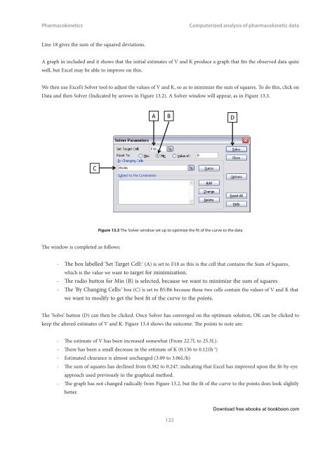
PharmacokineticsComputerized analysis of pharmacokinetic dataLine 18 gives the sum of the squared deviations.A graph in included and it shows that the initial estimates of V and K produce a graph that fits the observed data quitewell, but Excel may be able to improve on this.We then use Excel’s Solver tool to adjust the values of V and K, so as to minimize the sum of squares. To do this, click onData and then Solver (Indicated by arrows in Figure 13.2). A Solver window will appear, as in Figure 13.3.ABDCFigure 13.3 The Solver window set up to optimize the fit of the curve to the dataThe window is completed as follows:--The box labelled ‘Set Target Cell:’ (A) is set to F18 as this is the cell that contains the Sum of Squares,which is the value we want to target for minimization.--The radio button for Min (B) is selected, because we want to minimize the sum of squares--The ‘By Changing Cells:’ box (C) is set to B5:B6 because these two cells contain the values of V and K thatwe want to modify to get the best fit of the curve to the points.The ‘Solve’ button (D) can then be clicked. Once Solver has converged on the optimum solution, OK can be clicked tokeep the altered estimates of V and K. Figure 13.4 shows the outcome. The points to note are:--The estimate of V has been increased somewhat (From 22.7L to 25.3L).--There has been a small decrease in the estimate of K (0.136 to 0.121h -1 )--Estimated clearance is almost unchanged (3.09 to 3.06L/h)--The sum of squares has declined from 0.382 to 0.247, indicating that Excel has improved upon the fit-by-eyeapproach used previously in the graphical method.--The graph has not changed radically from Figure 13.2, but the fit of the curve to the points does look slightlybetter.122Download free ebooks at bookboon.com