Electrical conduction and Joule effect in one-dimensional chains of ...

More documents

Recommendations

Info

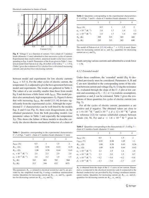
P. Béquin, V. Tournatof existing data on the dependence of electrical resistivityand thermal conductivity on temperature for stainless steels[22,25,26], and in particular for AISI 440C (code used bythe American Iron and Steel Institute) or 1.4125 (Europeanmaterial number).For small electric currents, the voltage V lc (between surfacesS 1 and S 2 )andthecurrentI are observed to be linearlydependent such as V lc = R lc I ,whereR lc is determined bythe slope of the U–I plot at low current (Fig. 2).The substitution of the first two terms of the Taylor expansionof ρλ ≃ ρ r λ r {1 + (α + β)(T − T r )} into Eqs. 3 and 4,leads to the potential difference between electrodes given byHolm [7]:V lc (T 0 ) = R lc I = ρ 0 2(n + 1) √ ρ r λ rρ r (α + β) 3 2{ []W(T 0 )× α arctan1 + (α + β)(T 0 − T r )}+ β W(T 0 )√where W(T 0 ) = α+β U(T0 )2(n+1) √ and ρρ r λ 0 = ρ r {1 + α(T 0 − T r )}.rBy introducing the maximum values of the electric currentI MAX and of the voltage U MAX ,Eq.6 can be rewritten as[]W(Tα arctan0 )1+(α+β)(T 0 −T r )+ β W(T 0 )I = I MAX [] , (7)α arctan+ β W MAXW MAX1+(α+β)(T 0 −T r )√ α+β UMAX2(n+1) √ ρ r λ r.where W MAX =Equations 6 and 7 give the relation between the current Iand the potential difference U between n beads, with α and βtwo parameters to be adjusted. For weak currents I in Eq. 6,the linear dependence between current and voltage is foundby imposing |β| ≪ α. Forhighercurrents,thefollowingsimplifications can be used:– the temperature T r associated to the reference variablesis equal to the temperature of the beads T 0 when theycarry a weak current I ;– the material at the contact follows the Wiedemann–Franz’s law which states that the product of the thermalconductivity by the electrical resistivity of a metalis proportional to the temperature: ρ r λ r = LT 0 ,whereL = 2.45 × 10 −8 V 2 /K 2 is the Lorenz number;– consequence of the preceding assumption, the quantityα + β must be close to 1/T 0 .Under these assumptions, the relation between the current Iand the voltage U can be written in the simplified form [7,8]:I = V lc(T 0 )= 2(n + 1)T √0 LR lc R lc× {αT 0 arctan [U(T 0 )] + (1 − αT 0 ) U(T 0 )} . (8)(6)where U(T 0 ) = U(T 0)2(n+1)T 0√L.4.1 DiscussionTo identify the limitations of the previous models (Eqs. 6 and8), experimental data (U, I ) obtained in a chain ofthree beads (diameter 11 mm) carrying a current with cyclesof increasing and decreasing values, are now presented.Figure 7 shows how voltage U and power P vary withcurrent I .From the preceding paragraph it can be seen that both Eqs.6 and 8, providingarelationbetweenthecurrentI and thevoltage U,presentasimilarform:I = A arctan(BU)+CU.Parameters A, B and C can be adjusted to obtain the best fitwith the experimental data, as shown in Figs. 6 and 8.4.1.1 Simplified modelsBy identifying parameters A, B and C to the correspondingterms of the simplified relation between current and voltage(Eq. 8), R lc , α and T 0 can be determined. Table 1 givesthe evolution of the latter quantities for successive cycles ofelectric current. Values of R lc are identical to those determinedby the slope of the U–I plot at low current (see valuesof R lc listed in Table 3). The values of α are positive anddecrease slowly with the current I MAX . This effect is discussedlater in this article. The values (α ≃ 2 × 10 −3 [K −1 ])are close to the values (α ≃ 6 × 10 −3 [K −1 ])giveninRef.[12]forvarioussolid/solidcontactsbetweenmetals(Al,Ni,Fe) and (α ≃ 1.6 × 10 −3 [K −1 ])giveninRef.[22] forastainless steel AISI 420. Finally, an important feature of thesimplified model is the prediction of temperatures T 0 of thebulk of the beads with anomalously high values comparedto the expected values around 300 K. This discrepancy maybe attributed to the use of Wiedemann–Franz’s law whichhas been found to be inadequate for some materials (iron andnickel for instance [8]).However, it is interesting to note that an equivalent formof this simplified model is used by Falcon et al. [13,14](Eq.(8) in Ref. [14]) and it correctly models the electro-thermalphenomena in the chain of stainless steel beads (martensiticstainless steel AISI 420). In this model [13,14], the coefficientα is initially deduced from the relation α −1 = 3.46 T 0(for an austenitic stainless steel AISI 304—see Ref. [26] from[14]) and is then replaced by the relation α −1 = 4 T 0 in orderto obtain a better agreement between predictions and experimentaldata for martensitic stainless steel beads AISI 420used in the experimental system.Figure 8 compares the experimental data (obtained in ourchain of 3 martensitic stainless steel beads AISI 440C) andthe model [13,14] with α −1 = 1.9 T 0 .Thislastexpressionwith factor 1.9 isfoundtoprovidethebestagreement123
Electrical conduction in chains of beadsTable 2 Quantities corresponding to the experimental characteristicsU–I of Figs. 7 and 8—chain of 3 stainless beads (diameter 11 mm)1 2 3 4I MAX (A) 0.5 1 1.5 2α ↓ ∗ 10 −3 (K −1 ) 1.8 1.7 1.4 1.2α ↑ ∗ 10 −3 (K −1 ) 1.8 1.7 1.4 0.9T 0↓ (K) 295 315 365 440T 0↑ (K) 295 315 365 600Fig. 8 Voltage U as a function of current I for a chain of 3 stainlessbeads (diameter 11 mm) submitted to four successive cycles of current.Experimental data (multisymbol), analytical model (solid lines) correspondingto Eqs. 6 and 8. Parameters of the fit are given in Table 3.Analyticalmodel from Falcon et al. (Eq. (8) in Ref. [14]) with α −1 = 1.9 T 0(Table 2 gives the evolution of T 0 ): (dashed lines with dotted) increasingcurrents and (dashed lines) decreasing currentsbetween model and experiments for low electric currentsI MAX = 0.5 A.Fortheothercyclesofelectriccurrent,thetemperature T 0 is adjusted to give the best agreement betweenmodel and experiments. The results are gathered in Table 2.The values of α are sensibly smaller than those from modelEq. 8 and decrease a little faster with I MAX .Thismodelpredictsalso anomalously high temperatures T 0 .Figure8 showsthat with increasing I MAX ,themodel[13,14] deviatessignificantlyfrom the experimental cycles. Although the experimentalU–I characteristics can be well fitted by the modelsEqs. 6 and 8 (see Fig. 8), there exist disagreements on theobtained parameters from the both preceding models (seeparameter values in Table 1 and especially the temperatureT 0 ). This shows the failure of these models to describe correctlythe electro-thermo-mechanical behavior of a chain ofTable 1 Quantities corresponding to the experimental characteristicsU–I of Figs. 7 and 8—chain of 3 stainless beads (diameter 11 mm)1 2 3 4I MAX (A) 0.5 1 1.5 2R lc↓ () 1.09 0.58 0.43 0.35R lc↑ () 1.08 0.58 0.44 0.41α ↓ ∗ 10 −3 (K −1 ) 2.4 2.3 2.0 2.0α ↑ ∗ 10 −3 (K −1 ) 2.4 2.2 1.9 1.5T 0↓ (K) 543 601 702 968T 0↑ (K) 513 544 632 1071The parameters R lc , α (related to electrical resistivity) and T 0 are providedby the simplified model Eq. 8 using a nonlinear minimizationroutine. Quantities for increasing current are R lc↑ , α ↑ and T 0↑ ; quantitiesfor decreasing current are R lc↓ , α↓ and T 0↓The model of Falcon et al. [13,14] withα −1 = 1.9 T 0 is used. Quantitiesfor increasing current are α ↑ and T 0↑ ; quantities for decreasingcurrent are α↓ and T 0↓beads carrying various currents and submitted to a weak force∼ 1N.4.1.2 Extended modelUnder these conditions, the ‘extended’ model (Eq. 6) describedpreviously must be considered. Parameters A, B andCarenowidentifiedtothecorrespondingtermsoftherelationbetween current and voltage (Eq. 6). Using the resistanceR lc evaluated through the slope of the U–I plot at low currentand assuming α(T 0 − T r ) ≪ 1 (a realistic assumption),quantities α and β can be estimated. Table 3 gives the evolutionsof these quantities for cycles of electric current (seeFig. 7).For all the cycles of electric current, parameters α arepositive and β negative. The obtained values are close toα ≃ 6×10 −3 K −1 and 2×10 −4 ≤ β ≤ 12×10 −4 K −1 givenby reference [12] forvarioussolid/solidcontactsbetweenmetals (Al, Ni, Fe) and α ≃ 1.6 × 10 −3 K −1 given inTable 3 Quantities corresponding to the characteristics U–I of Fig. 7—chain of 3 stainless beads (diameter 11 mm)1 2 3 4I MAX (A) 0.5 1 1.5 2U MAX (V) 0.93 0.98 1.05 1.1R lc↓ () 1.09 0.58 0.43 0.36R lc↑ () 1.09 0.58 0.44 0.42α ↓ ∗ 10 −3 (K −1 ) 2.2 1.9 1.4 1.0α ↑ ∗ 10 −3 (K −1 ) 2.3 2.0 1.5 0.7β ↓ ∗ 10 −4 (K −1 ) −5.2 −5.0 −4.2 −4.8β ↑ ∗ 10 −4 (K −1 ) −4.3 −3.6 −2.7 −2.5R lc is obtained from the slope of the U–I curve at low current. Parametersα (connected to the electrical resistivity) and β (connected to thethermal conductivity) are provided by Eq. 6 using a nonlinear minimizationroutine. Quantities for increasing current are R lc↑ , α ↑ and β ↑ ;quantities for decreasing current are R lc↓ , α ↓ and β ↓123
Page 5: Electrical conduction in chains of
Page 9 and 10: Electrical conduction in chains of
Page 11: Electrical conduction in chains of

Electrical conduction and Joule effect in one-dimensional chains of ...

Create successful ePaper yourself

Delete template?

Save as template?