Noise generated by cavitating single-hole and multi-hole orifices in ...

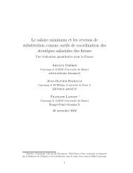
ARTICLE IN PRESSP. Testud et al. / Journal of Fluids and Structures 23 (2007) 163–189 165Fig. 1. Flow through an orifice and corresponding evolution of the static pressure.We prefer to use the cavitation number, based on the pressure drop across the singularity generating the jet:P vs ¼ P 2DP , (3)where DP ¼ P 1 P 2 is the pressure drop across the orifice, with P 1 the static pressure upstream of the orifice and P 2 thedownstream static pressure far away from the orifice. In this choice, we follow common practice in industry (Tullis,1989; Franc et al., 1999; Lecoffre, 1994).One should note that both those cavitation numbers lead to very similar classifications as they are related to eachother by the pressure drop coefficient of the singularity.When the pressure P j has a sufficiently low value, intermittent tiny cavitation bubbles are produced in the heart of theturbulent eddies along the shear layer of the jet. This flow regime transition is called cavitation inception, and it appearsat a cavitation number of the order of 1 (when d=D ¼ 0:30) according to the data of Tullis (1989). Other references(Numachi et al., 1960; Tullis and Govindajaran, 1973; Ball et al., 1975; Yan and Thorpe, 1990; Kugou et al., 1996; Satoand Saito, 2001; Pan et al., 2001) are in good agreement with the values and scale effects given by Tullis (1989). Somedifferences result from the influence of the variation in the dissolved gas content and in the viscosity (Keller, 1994).As the jet pressure decreases further, more bubbles with larger radii are generated, forming a white cloud. Thepressure fluctuations increase and a characteristic shot noise can be heard. A further decrease in jet pressure induces theformation of a large vapor pocket just downstream of the orifice, surrounding the liquid jet. The regime occurring afterthis transition is called super cavitation and it exhibits the largest noise and vibration levels. In the super cavitationregime, noise is known [see, for example, Van Wijngaarden (1972)], to be mainly generated in a shock transitionbetween the cavitation region and the pipe flow, at some distance downstream of the orifice. Downstream of the shock,some residual gas (air) bubbles can persist but pure vapor bubbles have disappeared.Cavitation indicators are used to predict the occurrence of cavitation regimes. The use of two of them has seemedrelevant, in view of our experimental results. First, a so-called incipient cavitation indicator, noted s i , which predicts thetransition from a noncavitating flow to a moderately cavitating flow, that is called developed cavitation regime. Second,a so-called choked cavitation indicator, noted s ch , which predicts the transition from a moderately cavitating flow to asuper cavitating flow, with the formation and continuous presence of a vapor pocket downstream of the orifice aroundthe liquid jet. To calculate both those incipient and the choked cavitation indicators, scaling laws are given by Tullis(1989). They take into account the various pressure effects and size scale effects, by means of extensive experiments onsingle-hole orifices in water pipe flow. For multi-hole orifices, as mentioned in the same work, less data are available butidentical values are expected to hold.Only a few studies provide downstream noise spectra generated by cavitating orifices (Yan et al., 1988; Bistafa et al.,1989; Kim et al., 1997; Pan et al., 2001). A few complementary studies give the noise spectra created by cavitating valves

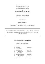
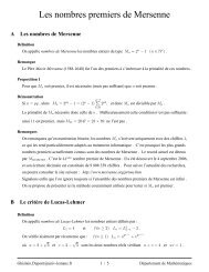
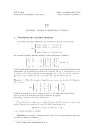
ARTICLE IN PRESS166P. Testud et al. / Journal of Fluids and Structures 23 (2007) 163–189(Hassis, 1999; Martin et al., 1981). In fact, it appears that far more research has been developed on submerged water jets(Jorgensen, 1961; Esipovand Naugol’nykh, 1975; Franklin and McMillan, 1984; Brennen, 1995; Latorre, 1997).A comprehensive overview of the state of the art in this domain is given in Brennen (1995).2. Experimental set-up2.1. Tested orificesIn the piping system of French nuclear power plants, a basic configuration to obtain a pressure discharge can berealized with a single-hole orifice. The maximum flow velocity can reach about 10 m s 1 and the pressure drop 100 baracross the orifice. This can induce high vibration levels. The orifices used are chosen in order to reduce the pipevibration to acceptable levels (Caillaud et al., 2006).In our study, two orifices have been tested (see Fig. 2), as follows:(i) A single-hole orifice, circular, centered, with right angles and sharp edges. It has a thickness of t ¼ 14 mm ðt=d ¼0:64Þ and a diameter of d ¼ 22 mm ðd=D ¼ 0:30Þ, for a pipe diameter of D ¼ 74 mm. It is considered as a ‘thin’orifice as t=dt2 (Idel’cik, 1969). In a sharp edged orifice flow, separation occurs at the upstream inlet edge. In athin orifice, there is no reattachment of the flow within the orifice.(ii) A multi-hole orifice, with N holes ¼ 47 circular right-angled and sharp-edged perforations of diameter d multi ¼ 3 mm.Its total open surface is practically identical to the single-hole orifice one, as it has an equivalent d eq =D ¼ 0:28 ratio.This multi-hole orifice also has the same thickness of t ¼ 14 mm ðt=d multi ¼ 4:67Þ. It behaves as a thick orificet=d\2. The flow reattaches to the wall within the orifice.2.2. Test rigThe test-section, as shown in Fig. 3, consists out of an open loop with a hydraulically smooth steel pipe of innerdiameter D ¼ 74 mm and wall thickness t p ¼ 8 mm. The orifices are placed between straight pipe sections with lengths,respectively, equal to 42 diameters upstream and 70 diameters downstream.The water is injected from a tank located 17 m upstream from the orifice. The nitrogen pressure in the tank above thewater is controlled by a feedback system to maintain a constant main flow velocity. The water is released at atmosphericpressure 20 m downstream of the orifice. The temperature is kept equal to 310 K ð1KÞ during all experiments.The flow velocity U is measured 26D upstream of the orifice, and the static pressures P 1 and P 2 are determined,respectively, by a transducer 11D upstream and another 40D downstream of the orifice. The fluctuating pressures aremonitored by means of a combination of Kistler 701A piezo-electrical transducers and Kistler charge amplifiers. Thelocation of the dynamical pressure transducers is given in Fig. 4. Upstream, the transducers 1–3 are positioned, atrespectively 11D, 8D and 5D from the orifice (0.25 m between consecutive transducers). Downstream, the transducers4–10 are regularly positioned, from 7D to 39D (0.4 m between consecutive transducers).Fig. 2. Front views of the tested orifices: (a) single-hole orifice; (b) multi-hole orifice.

ARTICLE IN PRESSP. Testud et al. / Journal of Fluids and Structures 23 (2007) 163–189 167Fig. 3. Scale scheme of the test rig.Fig. 4. Location of the dynamical pressure transducers upstream and downstream of the orifice.2.3. Experimental conditions2.3.1. Water qualityThe water used is tap water, demineralized, with pH 9 and weak conductivity. It is not degassed, hence it is expectedto be saturated with dissolved air. The volume fraction of dissolved gas (denoted by b) is high compared to othercavitation studies. This gas content has not been measured, but an estimation, assuming saturation condition under atemperature of T ¼ 310 K or T ¼ 273 K, gives for the volume fraction an order of magnitude around, respectively, 10 2or 10 3 .It should be pointed out that the presence of dissolved gas in the water does not mean a presence of gas bubbles in thewater. Thus, the measured upstream speed of sound does not reveal any presence of gas bubbles as it is close to the onein pure water flow.Correcting the compressibility of the water for the influence of the elasticity of the pipe (diameter D ¼ 7:4 10 2 m,wall thickness e ¼ 8 10 3 m, Young’s modulus E ¼ 2 10 11 Nm 2 , Poisson ratio z ¼ 0:3), the speed of sound c th inpure water in the pipe is given in function of the speed of sound in pure water c w (Lighthill, 1978):c th ¼ c w 1 þ r w c 2 Dð1 z 2 0:5Þw. (4)eEThis predicts a speed of sound of c th ¼ 1454 m s 1 using c w ¼ 1523 m s 1 . The measured speed of sound upstream of theorifice is 1420 10 m s 1 .2.3.2. Experimental flow conditionsExperiments are carried out at a constant flow by controlling the static pressure upstream of the orifice. Thedownstream pressure P 2 is imposed by the hydraulic static head of the 17.2 m high vertical pipe downstream of the

ARTICLE IN PRESS168P. Testud et al. / Journal of Fluids and Structures 23 (2007) 163–189orifice. Each experiment lasts about 90 s. Pressures and volume flows are provided in Table 1 for the six experiments onthe single-hole orifice, and in Table 2 for the six experiments on the multi-hole orifice.The Reynolds number Re ¼ UD=n water based on the pipe diameter and the water viscosity varies from 2 10 5 to5 10 5 ; turbulence is fully developed, as usual in industrial pipes.Higher flow regimes have been tested, but the pressure transducers downstream delivered no signal, as they werelocated in a vapor pocket characteristic of the super cavitation regime. As a consequence, no acoustic data are availablein these conditions, and the corresponding hydraulic conditions are not reported in Tables 1 and 2.2.4. Distinction of two cavitation regimesThe application of Tullis’ formulas to our experiments gives the cavitation indicators: s i for the developed cavitationand s ch for the super cavitation. Compared to our observations, those cavitation regime indicators are in goodagreement:(a) For the single-hole orifice: s i X0:93, s ch ¼ 0:25. The observations, based on listening and on the measureddownstream speed of sound, indicate that all experiments (i.e. so0:74) are cavitating. Furthermore, thedownstream acoustic properties and particularly the shape of the downstream noise spectra indicate that the lastthree experiments (i.e. so0:25) are in super cavitation regime.(b) For the multi-hole orifice: s i X0:87, s ch ¼ 0:20. The observations in this case indicate that all experiments (i.e.so0:74) are cavitating. The super cavitation regime is observed for the last two experiments (i.e. so0:17).Table 1Flow conditions for the single-hole orifice experiments (with standard deviations)Developed cavitationSuper cavitationU ðms 1 Þ 1.91 2.38 2.90 3.75 4.08 4.42St. deviation 0.06 0.04 0.04 0.03 0.03 0.05ðms 1 ÞP 1 ð10 5 PaÞ 6.3 9.2 13.3 21.4 25.0 29.5St. deviation 0.3 0.3 0.6 1.4 0.7 0.8ð10 5 PaÞP 2 ð10 5 PaÞ 2.7 2.7 2.7 2.8 2.8 2.8St. deviation 0.0 0.0 0.0 2.0 0.2 1.5ð10 5 PaÞs 0.74 0.41 0.25 0.15 0.12 0.10Table 2Flow conditions for the multi-hole orifice experiments (with standard deviations)Developed cavitationSuper cavitationU ðms 1 Þ 2.08 2.45 2.94 3.65 4.18 4.43St. deviation 0.02 0.04 0.04 0.02 0.02 0.04ðms 1 ÞP 1 ð10 5 PaÞ 6.5 6.9 12.9 19.8 26.0 28.3St. deviation 0.1 0.3 0.4 1.2 0.3 0.6ð10 5 PaÞP 2 ð10 5 PaÞ 2.7 2.8 2.8 2.9 3.0 0.9St. deviation 0.0 0.1 0.1 0.3 1.2 2.1ð10 5 PaÞs 0.74 0.45 0.28 0.17 0.13 0.03

2.5. Acoustic analysis methodARTICLE IN PRESSP. Testud et al. / Journal of Fluids and Structures 23 (2007) 163–189 169In the frequency range of the study, only acoustic plane waves propagate. The issue is to determine the spectra p þ andp representing, respectively, the upstream and downstream traveling plane waves and for which Fourier-like analysisholds.From each experiment, time fluctuating-pressure signals are obtained. These data are truncated to a time intervalwhere the acoustic properties do not evolve significantly, i.e. on a duration of about 10 s. With the help of a referencepressure p ref , we compute the cross-spectral densities G ppref ðf Þ, which are defined as the Fourier Transform of the timecorrelation (Bendat and Piersol, 1986). It is worth recalling that, for a small frequency bandwidth Df , the mean-squarevalue of the pressure in the frequency range ½f ; f þ Df Š is given by G pp ðf Þ Df . These cross-spectra are expressed inPa 2 =Hz. In order to get a spectral expression linear with the pressure, we choose to use the following expression, inPa=Hz 1=2 (see Appendix A for more details):p n ðf Þ¼G p n ðtÞp ref ðtÞðf Þpffiffiffiffiffiffiffiffiffiffiffiffiffiffiffiffiffiffiffiffiffiffiffiffiffiffið1pnp10Þ. (5)G pref ðtÞp ref ðtÞðf ÞFor upstream observations, transducer 1 is chosen as reference, and for downstream observations, transducer 10 ischosen as reference.As plane waves propagate, the acoustic pressure at one point is the summation of the forward (in the direction of theflow) traveling wave p þ and of the backward traveling wave p . We assume the speed of sound to be identical in theforward and in the backward directions, because the Mach number is low (of the order of 10 3 ). The identification ateach transducer of the local speed of sound and of the acoustic plane waves is carried out according to standardintensimetry techniques (Davies et al., 1980; Bode´ n and Abom, 1986; Hassis, 1999).The final spectra represent an average of about 20 spectra, determined with a time signal of 10 s duration. Eachintermediate spectrum is determined with a window of 1 s duration, and the successive windows have an overlappingratio of 0.5 (between 0 and 1). This average is made in order to reduce the random errors.The use of a single reference microphone may give uncertainties for determining standing waves if there is a pressurenode at a microphone. This happens when the reflection coefficient is close to unity. At low frequencies (below 500 Hz),this is the case for developed cavitation (see Fig. 6). However, as shown in Fig. 19, the microphones are not close to thepressure nodes of the standing wave patterns. At higher frequencies, and for super cavitation, the reflection coefficient isso low that we do not expect a problem (see Figs. 6 and 7).2.6. Acoustic boundary conditions on both sides of the orifice2.6.1. Acoustic boundary conditions upstream of the orificeThe acoustic conditions imposed by the test rig upstream of the orifice are quite reflecting, as illustrated in Fig. 5 bythe upstream reflection coefficient R ¼ p =p þ , defined as the ratio between the forward and the backward propagatingplane waves. These reflecting characteristics are due to multiple partial reflections of the acoustic waves on variouselements present on the upstream part of the test rig as an open valve, a few bends and section restrictions. Thoseelements have not been modified in the course of the experiments, so that these reflecting conditions not vary muchfrom one experiment to another.2.6.2. Acoustic boundary conditions downstream of the orificeThe downstream acoustic boundary condition depends on the cavitation regime, developed cavitation regime orsuper cavitation regime.In developed cavitation regime (see Fig. 6), the downstream reflection coefficient has a magnitude close to 1 up to600 Hz, which indicates a strong reflecting condition. As the phase is a linear function of the frequency, the reflectionpoint is determined: it corresponds to the location of an open valve (at 53D downstream of the orifice). The cavity ofthis valve is hence filled with a very compressible fluid, i.e. air, imposing an acoustic pressure node p 0 ¼ 0.The reflection coefficient shows values above unity in Figs. 5 and 6. This may be due to measurement inaccuracies.Also the presence of a noise source outside the main source region is possible and would give values above unity.In the super cavitation regime (see Fig. 7), the downstream reflection coefficient falls down below the value of 0.5. Asa first approximation, the pipe termination is then almost anechoic. This difference of behavior between the developedcavitation regime and the super cavitation regime is not analysed in the framework of the present study.This variation of the downstream acoustic boundary conditions is specific of the test rig. It has some impact on thelevels of the downstream spectra. This will be taken into account further in the study of the downstream noise spectra.

ARTICLE IN PRESS170P. Testud et al. / Journal of Fluids and Structures 23 (2007) 163–189piPhase (rad)0-pi10 500 1000 1500Amplitude1.21U=2.38 m.s -10.80.60.40.2010 500 1000 1500Frequency (Hz)Fig. 5. Typical acoustic reflection coefficient R ¼ pþpupstream of the orifice (calculated at transducer 1).It should be pointed out that, for some frequencies, the determination of the acoustical spectra is inaccurate. Butcoherence values are still good enough, as illustrated in Fig 8, to allow a satisfactory fit of the spectra to determine thespeed of sound, as illustrated in Fig. 9.3. Cavitation regimes3.1. Hydraulic model for the pressure drop DP across the single-hole orificeA simple model of the hydraulics of the single-hole orifice is proposed. The hydraulic conditions (pressure and Machnumber) at the jet of the orifice are estimated, hence giving some insight for a physical interpretation of the differentcavitation regimes.This hydraulic model is a simple classical Borda-Carnot model, see, for example Durrieu et al. (2001). It assumes anincompressible stationary single-phase flow, that is, no effect of cavitation on the hydraulics. Also, the ratio S j =Sbetween the free jet cross-section and the pipe cross-section S is considered as fixed.Firstly, mass conservation requiresS j U j ¼ SU. (6)Secondly, the flow upstream of the jet is assumed to be an inviscid steady potential flow, so thatP 1 þ 1 2 r wU 2 ¼ P j þ 1 2 r wU 2 j . (7)Downstream of the jet, a turbulent mixing region is followed by a uniform flow of velocity U. Neglecting friction at thewalls, and assuming a thin ðt=dt2Þ orifice (with no reattachment of the flow inside the hole of the orifice), one obtains(S d is the cross-section of the orifice)SP j þ r w U 2 j S j ¼ SP 2 þ r w U 2 S. (8)The pressure P j and the velocity U j at the jet are deduced from Eqs. (6)–(8). The measured pressure drop, denoted byDP measured , is in this case equal to the pressure drop across the orifice: DP measured ¼ P 1 P 2 . Hence, denoting by a thecontraction coefficient ða ¼ S j =S d Þ, this developed cavitation model gives" #DP measuredð1=2Þr w U 2 ¼ S 2 1 þ 2 2 S , (9)S jS j

ARTICLE IN PRESSP. Testud et al. / Journal of Fluids and Structures 23 (2007) 163–189 171piPhase (rad)0-pi10 500 1000 1500Amplitude1.210.80.60.40.2010 500 1000 1500Frequency (Hz)U=1.91 m.s -1Fig. 6. Typical acoustic reflection coefficient R ¼ p pþdownstream of the orifice (calculated at transducer 8) in developed cavitationregime.piPhase (rad)0Amplitude-pi10 500 1000 15001.210.80.60.40.2010 500 1000 1500Frequency (Hz)U=3.75 m.s -1Fig. 7. Typical acoustic reflection coefficient R ¼ p pþdownstream of the orifice (calculated at transducer 8) in super cavitation regime.the first part representing the dissipation from upstream to the jet, and the second part the dissipation from the jet todownstream.Finally, after simplifications, we findDP measuredð1=2Þr w U 2 ¼" # D 212 1d a. (10)

ARTICLE IN PRESS172P. Testud et al. / Journal of Fluids and Structures 23 (2007) 163–18910.90.80.7Coherence0.60.50.40.30.20.100 500 1000 1500 2000Frequency (Hz)Fig. 8. Example of the coherence function between two successive transducers (single-hole orifice, U ¼ 2:38 m s 1 , between transducers7 and 8).10.8(p 6 (ω)+p 8 (ω)) / p 7 (ω)fit with c=1425 m/s0.60.4cos (ω∆l/c)0.20-0.2-0.4-0.6-0.8-10 500 1000 1500 2000Frequency (Hz)Fig. 9. Example of the determination of the speed of sound using a fit on the spectra for three successive transducers (single-holeorifice, U ¼ 2:38 m s 1 , middle transducer: 7).In super cavitation, the downstream static sensor is in the jet region, measuring P j . The pressure drop measuredrepresents the dissipation from upstream to the jet (the first part of the preceding expression):DP measuredð1=2Þr w U 2 ¼ 1 D 4a 2 1. (11)d

ARTICLE IN PRESSP. Testud et al. / Journal of Fluids and Structures 23 (2007) 163–189 173320300280∆P measured / (0.5ρ w U 2 )260240220200single-hole experimentsthin-hole developed-cavitation model: α=0.65thin-hole super-cavitation model: α=0.651801 2 3 4 5 6 7 8U (m.s -1 )Fig. 10. Comparison between the Borda–Carnot model with different contraction coefficients a and the single-hole orificemeasurements.Table 3Conditions at the jet using the Borda–Carnot model for the single-hole orificeDeveloped cavitationSuper cavitationU ðms 1 Þ 1.91 2.38 2.90 3.75 4.08 4.42U j ðms 1 Þ 33 41 50 65 71 76c min ðms 1 Þ 28 30 34 13 — —P j ð10 5 PaÞ 1.4 1.6 2.0 0.3 — —Fig. 10 compares the two models using a contraction coefficient a ¼ 0:65 with experimental results (additionalexperimental results in super cavitation, not shown in Table 1, are plotted), as follows:(i) In the developed cavitation regime ðUo3:5ms 1 Þ, theory agrees qualitatively well with experiments, predicting DPwithin 15%.(ii) In the super cavitation regime ðU43:5ms 1 Þ, experimental data agree remarkably well with the model, predictingDP within 1%. Incidentally, we observe that super cavitation does not induce a strong slope variation in the DPversus U curve. This is mentioned in Tullis (1989) for orifices of low d=D ratio (approximately under 0.5, which isthe case here).As a result, the model is validated as a satisfying broad estimation of the hydraulics, taking a contraction coefficient of 0.65.This value is reasonable, as it is close to 0.61 which is the theoretical value for sharp-edged orifices with a jet from a gas to afree space exit (Gilbarg, 1960) and it is less than 0.70, which indicates (Blevins, 1984) that the real radius of curvature of theupstream edge of the orifice is less than 1% of the pipe diameter (this confirms that this edge is a neat sharp angle edge).Using this model, the pressure and the velocity at the jet are estimated, see Table 3, as follows:(a) The pressure in the jet P j is very close to the vapor pressure of the liquid ðP v ¼ 5:65 10 3 PaÞ in super cavitationregime. This is coherent with the stationary presence of a vapor pocket in this region. Hence, it may be an indicatorof the transition to super cavitation regime.(b) The velocity U j is compared to c min , an evaluation of the lowest speed of sound in the two-phase region of the jet.An estimation of it can be obtained, see Van Wijngaarden (1972): the minimum speed of sound is obtained for a

ARTICLE IN PRESSP. Testud et al. / Journal of Fluids and Structures 23 (2007) 163–189 175320300280∆P measured / (0.5ρ w U 2 )260240220200180160multi-hole experimentsthick-hole developed-cavitation model: α=0.65thin-hole developed-cavitation model: α=0.65thick-hole super-cavitation model: α=0.65single-hole experiments1401 2 3 4 5 6 7 8U (m.s -1 )Fig. 11. Evaluation of the multi-hole orifice model and comparison between the single-hole orifice measurements.Table 4Conditions at the jet using the Borda–Carnot model for the multi-hole orificeDeveloped cavitationSuper cavitationU ðms 1 Þ 2.08 2.45 2.94 3.65 4.18 4.43U j ðms 1 Þ 36 43 51 63 73 77c min ðms 1 Þ 20 — 27 — — —P j ð10 5 PaÞ 0.7 — 1.3 — —example in Fig. 14). The higher harmonics are typical of steady whistling stabilized by a nonlinear feedback effect as forall self-sustained oscillations (Fletcher, 1979; Rockwell and Naudascher, 1979).Scant literature has been found on whistling of cavitating orifices in pipes. A vortex shedding phenomenon inpresence of cavitation has been investigated by Sato and Saito (2001), but in the particular case of thick orificesðt=d\2Þ. On thin orifices, some visualizations (Moussou et al., 2003) made on other EDF experiments have shown thepossibility of the presence of vortex-shedding in cavitation regime, as can be seen in Fig. 15, from Archer et al. (2002).The whistling frequencies are given in Table 5. They do not increase continuously with the flow velocity, as one wouldexpect for a hydrodynamic oscillation edge-tone like (Blake and Powell, 1983). The stable frequency is typical of anacoustic feedback which creates and maintains the acoustic oscillation close to a resonance frequency. This is alsorevealed by the locking of the phase of the time pressure signals on successive sensors, which indicates a standing wavepattern.Upstream of the orifice, the level of whistling is higher than downstream: hence the acoustic feedback is suspected tohappen predominantly upstream. The upstream reflection coefficient, see Fig. 5, is reflecting but irregular: no clearacoustic reflection point can be identified (as it can be for the cavity of a valve downstream, see Section 2.6.2). Thisirregular shape is due to the intricacy of the upstream rig design, with a succession of elbows, slight restrictions ofsections and some open valves.It is also worth mentioning that the whistling frequency does not coincide with any downstream natural acousticfrequency. This is coherent with the acoustic uncoupling observed from both sides of the orifice.The single-hole orifice has a ratio t=d ¼ 0:6, inferior to 2, so that it is considered as a thin orifice. We assume that thewhistling phenomenon is influenced by the thickness of the orifice t, rather than its diameter. It is also natural to use the

ARTICLE IN PRESS176P. Testud et al. / Journal of Fluids and Structures 23 (2007) 163–189Fig. 12. From other experiments at EDF (Archer et al., 2002), visualization of the developed cavitation regime for a single-hole orifice(d=D ¼ 0:30, t=d ¼ 0:10, D ¼ 2:66 10 1 m) with s ¼ 0:49 and U ¼ 1:50 m s 1 (DP ¼ 3:1 10 5 Pa, P 1 ¼ 4:6 10 5 Pa). White bubbleclouds are observed around the jet formed at the orifice.Dynamical pressure signal at sensor 9 (10 5 Pa)2.521.510.50-0.5-1-1.5-2σ = 0.41-2.540 40.05 40.1 40.15Time (s)Fig. 13. Typical dynamical time pressure signal from a downstream transducer for the developed cavitation regime (here for the singleholeorifice at s ¼ 0:41).velocity at the orifice U d as a relevant scaling velocity. Hence the Strouhal number is defined asSt ¼ f 0tU d, (14)and values are reported in Table 5.

ARTICLE IN PRESSP. Testud et al. / Journal of Fluids and Structures 23 (2007) 163–189 17710 9 Frequency (Hz)10 8f 02 f 0U=1.91 m.s -1p− 2 (Pa 2 /Hz)10 710 610 510 40 200 400 600 800 1000Fig. 14. Detection of whistling frequency f 0 with harmonics on upstream plane wave spectra pU ¼ 1:91 m s 1 , f 0 ¼ 359 Hz and the first harmonics at 718 Hz).(here for the single-hole orifice atFig. 15. From other experiments at EDF (Archer et al., 2002), visualization of a cavitating and whistling single-hole orifice(d=D ¼ 0:30, t=d ¼ 0:10, D ¼ 2:6 10 1 m) with s ¼ 0:35 and U ¼ 1:97 m s 1 (DP ¼ 5:3 10 5 Pa, P 1 ¼ 7:2 10 5 Pa).The Strouhal number is obtained in the range 0.18–0.26. These values are close to data on orifices: Anderson (1953)finds a Strouhal number around 0.2 for whistling orifices in air with a free air exit. In Anderson’s experiments, theorifices were a bit thinner (with 0:2pt=Dp0:5, whereas here t=D ¼ 0:19) and the Reynolds numbers smaller(U d t=n air H10 3 with n air the kinematic viscosity of air, whereas here U d t=n water H10 5 ).The multi-hole orifice is a thick one, as t=d multi ¼ 4:7. Hence it is no surprise that it does not whistle. The flowreattaches itself inside each hole, which stabilizes the shear layers of the jet and hence prevents whistling in the samemanner as observed for the single-hole orifice.

ARTICLE IN PRESS178P. Testud et al. / Journal of Fluids and Structures 23 (2007) 163–189Table 5Strouhal number St ¼ f 0 t=U d of the whistling frequency f 0 (only observed in the single-hole orifice case)U ðms 1 Þ 1.91 1.91 2.38 2.38 2.90 2.90c ðms 1 Þ 1390 1200 660 1420 1130 1420f 0 (Hz) 359 397 421 436 427 434St 0.23 0.26 0.22 0.23 0.18 0.19Fig. 16. From other experiments at EDF, visualization of the super cavitation regime for a single-hole orifice.3.5. Super cavitation visualization and typical temporal signalIn the super cavitation regime, a vapor pocket is created in the jet region, as illustrated in Fig. 16.When the vapor pocket expands and reaches the downstream transducers, those transducers no longer deliver anyacoustical signal. This constitues an evidence for the existence of the vapor pocket.It appears that the length of the vapor pocket increases quickly with flow velocity. The length of the vapor pocketincreases from about 7D at U 0 ¼ 3:8ms 1 to 18D at U 0 ¼ 4:4ms 1 and is larger than 38D at U 0 ¼ 4:7ms 1 for thesingle-hole orifice. For the multi-hole orifice, the length of the vapor pocket increases from around 7D at U 0 ¼ 4:2ms 1to larger than 38D at U 0 ¼ 4:5ms 1 .The typical time-fluctuating pressure signals obtained are very different from those in the developed cavitation regime(see Fig. 17). They are asymmetric around the mean pressure, exhibiting very large positive spikes, up to 20 bar, linkedto the collapse of bubbles.Focusing on time signals (see an illustration in Fig. 18), it is seen that the phenomenon of bubble implosion ischaracterized first by a decrease in negative values of the fluctuating pressure with a characteristic duration of a tens ofmilliseconds, followed by an abrupt increase of the pressure, a ‘spike’, with a characteristic duration of 1 ms. Bymodeling this bubble volume evolution with a monopole source, which is a common and satisfactory simple model; see,for instance, Brennen (1995), the first decrease is linked with a decrease of the bubble size from its initial size to a valueclose to zero; the second part of the signal is linked with a pressure shock wave originating from the abrupt collision ofthe water particles. However, extremely high amplitudes are observed in comparison to Brennen (1995) (cf. Fig 3.19).This can be due either to the large size of our bubbles or to the effect of confinement.

ARTICLE IN PRESSP. Testud et al. / Journal of Fluids and Structures 23 (2007) 163–189 179Dynamical pressure signal at sensor 9 (10 5 Pa)20151050σ = 0.10-540 40.05 40.1 40.15Time (s)Fig. 17. Spurious pressure pulses (spikes) from collapsing bubbles on dynamical time pressure signal from a downstream transducer insuper cavitation regime (here for the single-hole orifice at s ¼ 0:10).2015Fluctuating pressure (x10 5 Pa)1050-547.07 47.075 47.08 47.085 47.09 47.095 47.1Time (s)Fig. 18. Cavitation peak in super cavitation regime (single-hole orifice at s ¼ 0:10).4. Results in the developed cavitation regimeThe single-hole and the multi-hole orifice developed cavitation regimes are presented together, as they show similaracoustical behavior. Firstly, results on the acoustic features of this cavitation regime are introduced: the observedvariations of the downstream speed of sound and the presence of resonance frequencies in downstream spectra. Thenthe downstream spectra, depending on those acoustical features, are presented and discussed.

ARTICLE IN PRESS180P. Testud et al. / Journal of Fluids and Structures 23 (2007) 163–1894.1. Acoustic features4.1.1. Spontaneous variations of the downstream speed of soundFor a fixed set of hydraulic conditions in the developed cavitation regime, the downstream speed of sound mayspontaneously evolve. For instance, the single-hole orifice experiment at U ¼ 2:38 m s 1 shows the downstream speed ofsound evolving from 660 m s 1 (during the first 20 s) to 1420 m s 1 (till the end of the experiment: 90 s).This variation of the speed of sound indicates that air bubbles are present, in varying quantity, in the water fardownstream of the orifice. For instance, a value of 660 m s 1 indicates a volume gas fraction in the water between 10 3and 10 4 , assuming the static pressure being between P j and P 2 [we use a classic formula; see, for example, VanWijngaarden (1972)]. On the contrary, a value of 1420 m s 1 indicates a negligible content of air in the water, as it isclose to the speed of sound in pure water [which equals to 1454 m s 1 , as presented in Section 2.3.1].Cavitation bubbles, when they are formed, are originally mainly constituted of vapor. During their lifetime, they aregradually filled with air, due to the diffusion of the dissolved gas present in the water surrounding them. As they driftdownstream, moving away from their region of creation, they reach regions where the pressure recovers higher levels.Pure vapor bubbles cannot persist, those bubbles remaining far downstream of the orifice are mainly filled with air (seefor example Fig. 12). Consequently, the observed variation of the quantity of air bubbles is suspected to be due to aninhomogeneity of the dissolved gas content in the injected water. This inhomogeneity may be related to temperaturevariations in the experimental installations. This hypothesis is all the more plausible as the water used has not receivedany degassing treatment, hence having a fluctuating and high dissolved gas content, not measured but estimated around10 2 or 10 3 (values at saturation conditions for T ¼ 273 and 310 K, respectively). In some experiments, the change inresidual air bubble content occurs after the water from the pipe segment between the orifice and the tank has beenevacuated and ‘fresh’ tank water has started to flow through the orifice.These variations of the downstream speed of sound during each experiment have some influence on the acousticalbehavior downstream of the orifice: the values of the natural frequencies, appearing downstream, are alteredproportionally with the speed of sound.The propagating waves are subjected to two-phase flow damping, as already mentioned by Hassis (1999). As regards thislast effect, no significant variation of the propagating wave amplitude could be measured along the downstream sensors,but the downstream acoustical reflection coefficient appears to vary significantly with the downstream speed of sound.4.1.2. Acoustical uncoupling from both sides of the orificeAn acoustical uncoupling is observed between acoustical spectra upstream and downstream of the orifice: the naturalfrequencies present downstream are strongly attenuated on upstream spectra; the whistling, when present, is visible onupstream spectra, but hardly on downstream spectra; and, furthermore, the background noise on downstream spectra is higherthan the one on upstream spectra, approximately from a factor 2 (for U ¼ 1:91 m s 1 ) up to 7 (for U ¼ 2:90 m s 1 )forthesingle-hole orifice, and much more significantly for the multi-hole orifice, with an approximately constant factor of about 10.This acoustical uncoupling is an effect of cavitation as there is choking (indicated in Table 3).4.1.3. Presence of natural modes downstreamIn this developed cavitation regime, resonance frequencies are systematically observed in acoustical spectradownstream of the orifice (both for the single-hole and the multi-hole).The acoustic boundary conditions are of a similar type, as the frequencies are of the form: f n ¼ nf 1 , f 1 being the firstresonance frequency. More precisely, these acoustic boundary conditions can be identified by extrapolating the standingwave patterns at those resonance frequencies. This extrapolation is made possible as a series of transducers (7 innumber) is present downstream of the orifice. As a result, we find two acoustic pressure nodes p 0 ¼ 0 (see Fig. 19),discussed above, as follows:(i) One acoustic pressure node is found far downstream of the orifice, at 52D ð1DÞ. It is the result of the influence of acavity of an open valve filled with air. The reflection coefficient imposed by such a cavity has been presented inFig. 6. The magnitude of the reflection coefficient jRj is close to 1, which confirms the acoustic influence of this cavity.(ii) Another is found just downstream of the orifice, at 4D ð1DÞ. It is likely to be caused by a cavitation cloud.4.2. Noise spectra generated downstreamNoise spectra generated in the pipe downstream of the orifice for the developed cavitation regime are presented in thissection.

ARTICLE IN PRESSP. Testud et al. / Journal of Fluids and Structures 23 (2007) 163–189 181Real part of the cross-spectra (Pa/Hz 0.5 )1.510.50-0.5-1x 10 4p’~0p’~0-1.5-1 0 1 2 3 4 5↑ Orifice↑ Downstream valveDistance (m)Fig. 19. In the developed cavitation regime, two acoustic boundary conditions p 0 ’ 0 are found downstream of the orifice, hencenatural frequencies appear, pointed out by the interpolation of the values of the cross-spectra at those first natural frequencies (here forthe single-hole orifice at U ¼ 2:38 m s 1 , c ¼ 1420 m s 1 and five natural frequencies: 188 Hz, m 386 Hz, . 574 Hz, ’ 770 Hz,E 957 Hz).The downstream transducers give a far-field measurement, as they are not located in the source region mainlyconstituted of bubble implosions located just downstream of the orifice. The acoustical power measured at downstreamtransducers represents the noise generated in the pipe. Under the assumptions of plane-wave propagation and noinfluence of the flow (the Mach number is around 10 3 ), the acoustical power takes the expression: Sðp þ2 p 2 Þ=ðr w c w Þ(Morfey, 1971).It is furthermore assumed that the backward propagating wave spectrum of p is small enough to be neglected. Evenif acoustical reflection is observed to occur downstream, this estimation of the source of noise is considered satisfactoryenough as an order of magnitude (this is all the more relevant as logarithmic representation is used). Thus, it comes tothe source power being represented by the quantity Sp þ2 =ðr w c w Þ.Of course, this representation is no more valid for the discrete frequencies which are whistling harmonics andresonance frequencies, as the backward propagating wave has great influence in those cases.The acoustical power spectra obtained downstream of the orifice for the developed cavitation regime are given inFig. 20 for the single-hole orifice and in Fig. 21 for the multi-hole orifice. The rejection frequency corresponding to awavelength of half of the distance between two successive transducers and depending on the measured speed of soundhas been excluded from those results. The following observations are made on those spectra:(a) spectra exhibit a hump form in the upper frequency range (above 200 Hz); this hump form is typical of cavitationalnoise (Martin et al., 1981; Brennen, 1995);(b) the single-hole orifice generates remarkably much more noise (by a factor of about 10 2 in the acoustical power) thanthe multi-hole orifice.4.3. Nondimensional analysis and representation4.3.1. Choice of the scaling variables for the noise spectraScaling is proposed in order to obtain a dimensionless representation of the acoustical source power.Cavitation noise from the implosions of bubbles is assumed to be predominant in order to scale the noise spectra.Hence, broadband turbulence noise from the mixing region downstream, whistling and resonance frequencies are not

ARTICLE IN PRESS182P. Testud et al. / Journal of Fluids and Structures 23 (2007) 163–18910 0 f (in Hz)10 -1S p +2 /(ρ w c) (in W/Hz)10 -210 -310 -410 -510 -6σ=0.74, c=1280 m/sσ=0.41, c=660 m/sσ=0.25, c=1430 m/s10 1 10 2 10 3Fig. 20. Acoustical power spectra in developed cavitation (single-hole orifice).10 -1 f (in Hz)10 -2p+ 2 S/(ρ c) (in W/Hz)10 -310 -410 -510 -610 -7σ=0.74, c=1420 m/sσ=0.45, c=1420 m/sσ=0.28, c=1425 m/sσ=0.17, c=1425 m/s10 1 10 2 10 3Fig. 21. Acoustical power spectra in developed cavitation (multi-hole orifice).taken into account to choose the scaling variables. This assumption of predominance of cavitation noise is globallyvalid, but seems to fail at low frequencies (in this work, below 200–300 Hz approximately). Also, it is assumed thatwhistling does not alter cavitation noise, generalizing the hypothesis that broadband noise is not affected by whistling[as shown in Verge (1995) for a flue organ pipe].Following Blake (1986), the amplitude of noise produced by cavitation should be made dimensionless by dividingwith the downstream pressure, and not the pressure drop, when using a Rayleigh–Plesset bubble dynamic model for aspherical isolated free bubble. However, ring vortices generated by an orifice are not isolated bubbles in free space, so

ARTICLE IN PRESSP. Testud et al. / Journal of Fluids and Structures 23 (2007) 163–189 183Fig. 22. Choice of the variables d and U d for the scaling of the noise spectra in the developed cavitation regime for the single-holeorifice.that this scaling should not hold in the case of the present study, as it also does not for sheet cavitation on airfoils(Keller, 1994).As we lack a precise model, the scaling data are chosen for the sake of simplicity: the basic idea, as shown in Fig. 22,relies on the fact that, in the developed cavitation regime, the bubbles are created in the mixing high-shear region of thejet.For the single-hole orifice experiments, the velocity U d and the orifice diameter d are representative of the conditionsin this region, hence those quantities are used in order to scale the noise spectra in this regime. Furthermore, the scalingpressure is defined as the pressure drop DP across the orifice, which is a measure of the kinetic energy density in the jet.Hence for the single-hole orifice in developed cavitation, fd=U d is the nondimensional frequency and p þ2 U d =ðDP 2 dÞ isthe nondimensional magnitude.For the multi-hole orifice experiments, we assume the noise issuing from incoherent N holes sources.Each source represents the radiation of one hole. It radiates on a characteristic surface of S=N holes . The strength ofeach source is assumed to be independent of the environment of the source. This assumption is natural, as we havepreviously supposed (see previous section) that the noise generated by the single-hole orifice does not depend on thediameter of the pipe. However, it should be pointed out that this assumption is wrong when whistling occurs.In this model, the total acoustic power P measured downstream is a summation of the acoustic power P each sourceemitted by each source [the key element is that sources are supposed to be incoherent between each other, see Pierce(1981)]:P ¼ N holes P each source . (15)The acoustic power of each source P each source is, by definition, the total acoustic intensity flux I multiplied the surface ofthis source:P each source ¼ IS=N holes . (16)Hence the total acoustic power isP ¼ SI. (17)The total acoustic power is consequently independent of the number of holes. As previously, we ignore any downstreamreflections, so that I ¼ p þ2 =ðrcÞ.This argumentation based on energy considerations can also be conducted in terms of forces: if the source isrepresented as a force acting on the orifice, taking the form Sp þ , the total force imposed on the multi-hole orifice is dueto the contribution of the forces imposed by N holes equivalent single-hole orifices with open surface S=N holes . Thoseforces are supposed to be uncorrelated with each other. Thus, the total force squared equals N holes times the forcesquared due to one hole. As the force squared of one hole is ðp þ S=N holes Þ 2 , the total force squared is expressed as:N holes ðp þ S=N holes Þ 2 , or by simplifying: ðp þ SÞ 2 =N holes .The scaling of the acoustic power is based on each source of surface S=N holes . The scaling velocity is the velocity atthe orifice, which is taken equal to the velocity of the single-hole orifice U d , as the open surface of the two orifices arevery similar, and the scaling length is the diameter of one hole d multi . In conclusion for the multi-hole orifice indeveloped cavitation: fd multi =U d is the nondimensional frequency, and p þ2 U d =ðDP 2 d multi Þ is the nondimensionalmagnitude.4.3.2. Nondimensional noise spectra generated downstreamThe dimensionless acoustical power spectra obtained downstream of the orifice for the developed cavitation regimeare given in Fig. 23 for the single-hole orifice and in Fig. 24 for the multi-hole orifice. The following observations areworth noting.

ARTICLE IN PRESS184P. Testud et al. / Journal of Fluids and Structures 23 (2007) 163–18910 0 f d/U d (10

ARTICLE IN PRESSP. Testud et al. / Journal of Fluids and Structures 23 (2007) 163–189 185(b) The different scaling used for the single-hole and the multi-hole orifice is rather efficient as it makes the levels of thetwo types of orifices closer to each other. However, the nondimensional level of noise of the single-hole orifice is stillhigher, with a ratio of 10, than the one of the multi-hole orifice experiments; see Figs. 23 and 24.(c) We compare the cavitation noise with a standard turbulence noise from a noncavitating orifice in the low frequencyrange. Indeed, in this range of frequency, the level of noise is expected to be mainly determined by turbulence noise(Martin et al., 1981). We use a nondimensional turbulence noise level proposed by Moussou (2005). In this model,the scaling is based on empirical data obtained with simple singularities (single-hole orifice, valve) in water-pipeflow: the level of noise is assumed to depend only on a Strouhal number based on the pipe diameter and thepipe flow velocity. We apply this model with the values of the pipe diameter D and a pipe flow velocity of 2:20 m s 1and compare it to the single-hole orifice nondimensional noise, see Fig. 23. As expected, the turbulence levelfits rather well the cavitation noise at low frequencies, with a good estimation of the slope; the cavitation noise ismuch stronger than the turbulence noise above the low-frequency range, which is a well-known result Brennen(1995).5. Results in the super cavitation regime5.1. Acoustic featuresThe super cavitation experiments exhibit two main differences compared to the developed cavitation experiments, asfollows:(i) The downstream speed of sound appears to be quite constant during each experiment.(ii) No resonance frequencies are found on downstream spectra. The downstream reflection coefficient is much lowerthan in the developed cavitation case (as previously shown in Fig. 7). In this case, the cavity of the downstreamvalve does not reflect the acoustic waves.As for the developed cavitation case, strong acoustic uncoupling is observed from both sides of the orifice. The effectis much more obvious here, with an average ratio between downstream and upstream power spectra of about 2–30 forthe single-hole orifice case, and about 10–50 for the multi-hole orifice case.5.2. Noise spectra generated downstreamNoise spectra obtained downstream are given in Fig. 25 for the single-hole orifice and in Fig. 26 for the multi-holeorifice (as previously, the rejection frequencies being excluded). We note the following points:(i) The typical cavitational hump form is observed, as in the developed cavitation case, but with much more evidence.The level of the hump is higher than for the developed cavitation regime; also, the frequency peak is smaller: thosetendencies when the cavitation number increases confirm literature data Brennen (1995).(ii) Also, as in the developed cavitation case, the single-hole orifice is clearly more noisy (with an approximate factor of10 on acoustical power spectra) than the multi-hole orifice.An important result is illustrated in Figs. 26 and 27: the part of the spectra succeeding the hump peak frequencydepend strongly on the downstream speed of sound. Two-phase flow attenuations phenomena are supposed to be thecause of this observation.6. ConclusionA single-hole and a multi-hole cavitating orifice in a water pipe have been studied experimentally under industrialconditions, i.e. with a pressure drop varying from 3 to 30 bar and a cavitation number in the range 0:03psp0:74.In the regime of developed cavitation, whistling is observed for the single-hole orifice. This occurs at a Strouhalnumber based on the orifice thickness with a value close to 0.2.Our results indicate that in the developed cavitation regime, a multi-hole orifice is much more silent than a single-holeorifice with the same total cross-sectional opening. This might be partially explained by the absence of correlation

ARTICLE IN PRESS186P. Testud et al. / Journal of Fluids and Structures 23 (2007) 163–189between the sound produced by different holes in the absence of whistling. No such difference is found in supercavitation. This is explained by the fact that, in the super cavitation regime, sound is produced far downstream of theorifice rather than in a near region downstream of the orifice.A nondimensional noise source is proposed for the developed cavitation regime (cf. Section 4.3). The source modelseems satisfactory for the developed cavitation case.The results presented are certainly limited and call for further research. In particular, it could be interesting to varythe shape of the orifices and repeat the experiments with degassed water.10 1 f (in Hz)10 0p+ 2 S/ (ρ c) (in W/Hz)10 -110 -210 -310 -4σ=0.15, c=280 m/sσ=0.15, c=1420 m/sσ=0.12, c=120 m/sσ=0.12, c=1310 m/sσ=0.10, c=1230 m/sσ=0.10, c=340 m/s10 1 10 2 10 3Fig. 25. Acoustical power spectra in super cavitation (single-hole orifice).10 1 f (in Hz)10 0p+ 2 S/ (ρ c) (in W/Hz)10 -110 -210 -310 -4σ=0.03, c=1400 m/sσ=0.13, c=1010 m/sσ=0.13, c=700 m/s10 1 10 2 10 3Fig. 26. Acoustical power spectra in super cavitation (multi-hole orifice).

ARTICLE IN PRESSP. Testud et al. / Journal of Fluids and Structures 23 (2007) 163–189 18710 1 f (in Hz)10 0p+ 2 S/ (ρ c) (in W/Hz)10 -110 -210 -310 -4σ=0.15, c=1420 m/sσ=0.15, c=1300 m/sσ=0.15, c=610 m/sσ=0.15, c=280 m/s10 1 10 2 10 3Fig. 27. Super cavitation (single-hole orifice): influence of the speed of sound on the noise spectra.AcknowledgmentThe experiments have been designed and realized by MM. S. Caillaud, Ch. Martin and L. Paulhiac.Appendix A. Acoustic analysisWe assume that only plane waves propagate in the pipe. First, cross-spectral density functions G ppref are used. They arewell suited to acoustic analysis, because they eliminate nonpropagating noise present in time measurements. Indeed, if wedecompose time pressure measurements pðtÞ into a nonpropagating signal p nonprop ðtÞ and a propagating one, we havepðtÞ¼p þ ðtÞþp ðtÞþp nonprop ðtÞ.(A.1)Having defined and fixed a reference sensor and applying the cross-spectral density functions, we get an expression where thenonpropagating pressure is removed because it is not correlated to the propagating pressure:G pðtÞpref ðtÞðoÞ¼G p þ ðtÞp ref ðtÞðoÞþG p ðtÞpref ðtÞðoÞ.(A.2)pSecond, we define quantities G ppref =ffiffiffiffiffiffiffiffiffiffiffiffiffi G pref p refwhich can be handled like Fourier Transforms, and which are almostindependent of the reference pressure. Indeed, if we assume a perfect coherence between the point of observation and thereference sensor, we havejG ppref j 2¼ 1. (A.3)G pp G pref p refpIn this case the quantity G ppref =ffiffiffiffiffiffiffiffiffiffiffiffiffi G pref p refdoes not depend on the reference sensor. In practice, the reference sensor is takenclosest to the points of observation.Finally, we calculate plane waves. Considering two consecutive sensors, denoted n and n þ 1, plane wavespropagation and the linearity characteristics of the cross-spectral density function giveG p þnþ1 p ref ðoÞ ¼G p þ n p refðoÞe jot ,G pnþ1 p refðoÞ ¼G pn p refðoÞe þjot ,(A.4)(A.5)

188ARTICLE IN PRESSP. Testud et al. / Journal of Fluids and Structures 23 (2007) 163–189pwith t being the time of flight of the wave between the two sensors. For the sake of ease, we note p n for G pn p ref=ffiffiffiffiffiffiffiffiffiffiffiffiffiffi G pref p ref.By means of Eqs. (A.2), (A.4) and (A.5), we get the plane wave spectra:p þ n ðoÞ ¼p nðoÞ e þjot þ p nþ1 ðoÞ, (A.6)2j sinðotÞp n ðoÞ ¼ p nðoÞ e jot þ p nþ1 ðoÞ, (A.7)2j sinðotÞfor p upstream measurements ð1pnp2Þ and downstream measurements ð4pnp9Þ. These spectra are expressed inPa=ffiffiffiffiffiffiHz .The reflection coefficient is defined as p =pþ downstream of the orifice, and by p þ =p upstream, because weassume the source of sound to be located in the region of the orifice. For example, if a zero pressure condition is locatedfar downstream of the orifice, and if T is the time of flight toward this pressure node, the reflection coefficient at thiscurrent point is e 2joT .ReferencesAnderson, A.B.C., 1953. A circular-orifice number describing dependency of primary Pfeifenton frequency on differential pressure, gasdensity and orifice geometry. Journal of the Acoustical Society of America 25, 626–631.Archer, A., Boyer, A., Nimanbeg, N., L’Exact, C., Lemercier, S., 2002. Re´ sultats des essais hydrauliques et hydroacoustiques du tronconPTR 900 sur la boucle EPOCA (in French). EDF R&D, Technical Note HI-85/02/023/A, France.Au-Yang, M.K., 2001. Flow-Induced Vibration of Power and Process Plant Components: A Practical Workbook. ASME Press, NewYork.Ball, J.W., Tullis, J.P., Stripling, T., 1975. Predicting cavitation in sudden enlargements. ASCE Journal of the Hydraulics Division 101,857–870.Bendat, J.S., Piersol, A.G., 1986. Random Data—Analysis and Measurement Procedures, second ed. Wiley-Interscience, New York,ISBN 0-471-04000-2.Bistafa, S.R., Lauchle, G.C., Reethof, G., 1989. Noise generated by cavitation orifice plates. ASME Journal of Fluids Engineering 111,278–289.Blake, W.K., 1986. Mechanics of Flow-Induced Sound and Vibration, vol. II. Academic Press, Orlando.Blake, W.K., Powell, A., 1983. The development of contemporary views of flow-tone generation. In: Recent Advances inAeroacoustics, Springer, New York.Blevins, R., 1984. Applied Fluid Dynamics Handbook. Krieger, New York ISBN 0-89464-717-2.Bodén, H., Abom, M., 1986. Influence of errors on the two-microphone method for acoustic properties in ducts. Journal of theAcoustical Society of America 79 (2).Brennen, C.E., 1995. Cavitation and Bubble Dynamics. Oxford University Press, Oxford.Caillaud, S., Gibert, J.R., Moussou, P., Cohen, J., Millet, F., 2006. Effect on pipe vibrations of cavitation in an orifice and in globestylevalves. In: ASME Pressure Vessels and Piping Division Conference, Proceedings PVP2006-ICPVT11-93882, Vancouver,Canada.Davies, P.O.A.L., Bhattacharva, M., Bento Coelho, J.L., 1980. Measurement of plane wave acoustic fields in flow ducts. Journal ofSound and Vibration 72, 539–542.Durrieu, P., Hofmans, G., Ajello, G., Boot, R., Aurégan, Y., Hirschberg, A., Peters, M.C.A.M., 2001. Quasisteady aero-acousticresponse of orifices. Journal of the Acoustical Society of America 110 (4), 1859–1872.Esipov, I.B., Naugol’nykh, K.A., 1975. Cavitation noise in submerged jets. Soviet Physics Acoustics 21, 404–405.Fletcher, N.H., 1979. Excitation mechanisms in woodwind and brass instruments. Acustica 43, 63–72.Franc, J.P., Avellan, F., Belahadji, B., Billard, J.Y., Brianc-on-Marjollet, L., Fréchou, D., Fruman, D.H., Karimi, A., Kueny, J.L.,Michel, J.M., 1999. La cavitation (in French). ISBN 2.7061.0605.0, Presses Universitaires de Grenoble.Franklin, R.E., McMillan, J., 1984. Noise generation in cavitating flows, the submerged jet. ASME Journal of Fluids Engineering 106,336–341.Gilbarg, G., 1960. Jets and cavities. In: Pflu¨ gge, S. (Ed.), Handbuch der Physik, vol. 9. Springer, Berlin, pp. 311–445.Hassis, H., 1999. Noise caused by cavitating butterfly and monovar valves. Journal of Sound and Vibration 225, 515–526.Idel’cik, I.E., 1969. Memento des pertes de charge (in French). Eyrolles, Paris.Jorgensen, D.W., 1961. Noise from cavitating submerged water jets. Journal of the Acoustical Society of America 33 (10), 1334–1338.Keller, A.P., 1994. New scaling laws for hydrodynamic cavitation inception. In: Second International Symposium On Cavitation,vol. 2, Tokyo, Japan, pp. 327–334.Kim, B.C., Pak, B.C., Cho, C.H., Chi, D.S., Choi, H.M., Choi, Y.M., Park, K.A., 1997. Effects of cavitation and plate thickness onsmall diameter ratio orifice meters. Flow Measurement and Instrumentation 8, 85–92.

ARTICLE IN PRESSP. Testud et al. / Journal of Fluids and Structures 23 (2007) 163–189 189Kugou, N., Matsuda, H., Izuchi, H., Miyamoto, H., Yamazaki, A., Ogasawara, M., 1996. Cavitation characteristics of restrictionorifices. ASME Fluids Engineering Division Conference, FED-vol. 236 (1), San Diego, California, pp. 457–462.Latorre, R., 1997. Bubble cavitation noise and the cavitation noise spectrum. Acta Acustica 83, 424–429.Lecoffre, Y., 1994. La cavitation, traqueurs de bulles (in French). Hermes, Paris, ISBN 2-86601-409-X.Lighthill, J., 1978. Waves in Fluids. Cambridge University Press, Cambridge.Martin, C.S., Medlarz, H., Wiggert, D.C., Brennen, C.E., 1981. Cavitation inception in spool valves. ASME Journal of FluidsEngineering 103, 564–576.Morfey, C.L., 1971. Acoustic energy in non-uniform flows. Journal of Sound and Vibration 14, 159–170.Moussou, P., 2005. An attempt to scale the vibration of water pipes. Proceedings 71217 of PVP, ASME, Denver, Colorado, USA.Moussou, P., Caillaud, L., Villouvier, V., Archer, A., Boyer, A., Rechu, B., Benazet, S., 2003. Vortex-shedding of a multi-hole orificesynchronized to an acoustic cavity in a PWR piping system. In: PVP-vol. 465, Flow-Induced Vibration PVP2003-2086, ASMEPress, New York, pp. 161–168.Moussou, P., Cambier, C., Lachene, D., Longarini, S., Paulhiac, L., Villouvier, V., 2001. Vibration investigation of a French PWRpower plant piping system caused by cavitating butterfly valves. In: PVP-vol. 420–2, Flow-Induced Vibration: Axial Flow, PipingSystems, Other Topics, ASME Press, New York, pp. 99–106.Moussou, P., Lafon, Ph., Potapov, S., Paulhiac, L., Tijsseling, A., 2004. Industrial cases of FSI due to internal flows. In: NinthInternational Conference on Pressure Surges, Chester (UK), vol. 1. pp. 167–184, BHR Group Limited.Numachi, F., Yamabe, M., Oba, R., 1960. Cavitation effect on the discharge coefficient of the sharp-edged orifice plate. ASMEJournal of Basic Engineering 82, 1–11.Pan, S.S., Xiang, T., Wu, B., 2001. Investigating to cavitation behavior of orifice tunnel. CAV2001, Fourth Symposium on Cavitation,California Institute of Technology, Pasadena, USA hhttp://cav2001.library.caltech.edu/222i.Pierce, A.D., 1981. Acoustics: An Introduction to its Physical Principles and Applications. McGraw-Hill Book Company Inc.,New York.Rockwell, D., Naudascher, E., 1979. Self-sustained oscillations of impinging free shear layers. Annual Review of Fluid Mechanics 11,67–94.Sato, K., Saito, Y., 2001. Unstable cavitation behavior in a circular–cylindrical orifice flow. CAV2001, Fourth Symposium onCavitation, California Institute of Technology, Pasadena, USA hhttp://cav2001.library.caltech.edu/318i.Tullis, J.P., 1989. Hydraulics of Pipelines: Pumps, Valves, Cavitation, Transients. Wiley Interscience Ed., New York.Tullis, J.P., Govindajaran, R., 1973. Cavitation and size scale effects for orifices. ASCE Journal of the Hydraulics Division 99,417–430.Van Wijngaarden, L., 1972. One-dimensional flow of liquids containing small gas bubbles. Journal of Fluid Mechanics 16, 369–396.Verge, M.P., 1995. Aeroacoustics of confined jets. Thesis, Technische Universiteit Eindhoven, The Netherlands, ISBN-90-386-0306-1.Weaver, D.S., Ziada, S., Au-Yang, M.K., Chen, S.S., Padoussis, M.P., Petitgrew, M.J., 2000. Flow-induced vibration of power andprocess plant components: progress and prospects. ASME Journal of Pressure Vessel Technology 122, 339–348.Yan, Y., Thorpe, R.B., 1990. Flow regime transitions due to cavitation in the flow through an orifice. International Journal ofMultiphase Flow 16 (6), 1023–1045.Yan, Y., Thorpe, R.B., Pandit, A.B., 1988. Cavitation noise and its suppression by air in orifice flow. In: Symposium on Flow-InducedNoise, Chicago, Ill., vol. 6. ASME, New York, pp. 25–39.Young, F.R., 1999. Cavitation. Imperial College Press, London ISBN 1-86094-198-2.