2 The scaling of MOSFETs, Moore's law, and ITRS

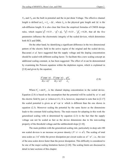
The scaling of MOSFETs, Moore’s law, and ITRS Chapter 2V bi and V ds are the built in potential and the in put drain Voltage. The effective channellength is defined as L el= L g− ∆ L , where L g is the physical gate length and ∆L is thesub-diffusion length. It is also clear that from the empirical formulas of CMOS designxrules, which requirejtL ≈ 0.33 , ox 1 WL ≈ dVT30 L ≈ 0.33 , V ≈ 0.20 , that all the fiveparameters influence the electrostatic integrity of the scaled devices, which determinesboth SCE and DIBL.On the other hand, by identifying a significant difference in the two dimensionalpattern of the electric field in the active region of the original and the scaled device,Baccarani et al. have suggested that the supply voltage and the doping concentrationshould be scaled with different scaling factor. To facilitate this a new scaling concept anadditional scaling constant, α, has been suggested. The effect of α can be demonstratedby examining the Poisson equation within the depletion region, which is explained in[2:8] and given by the equation:dd∂ ( αψ / κ) ∂ ( αψ / κ)qN2 2'a+ =2 2∂( x / κ ) ∂( y / κ)εsi(2.8)Where N'a= ακ N , is the channel doping concentration in the scaled device.aEquation (2.8) is based on the assumption that the potential will be scaled by α / κ andthe electric field by just α (whereα ≥1). It is, however, important to note that in [2.17]the scaled potential is given as ψ ' = ψ / κ which is different than the one shown inequation (2.3). Moreover scaling the potential by the same factor as the dimensionsleads to the constant field scaling theory. The main reason for adopting in this work thegeneralised scaling with α determined by equation (2.3) is the fact that the supplyvoltage can not be scaled as fast as the device dimensions due to the non-scalingproperty of the threshold voltage and the subthreshold slope [2.10].The main problem with the generalized scaling rule, particularly in deep sub-100nm scaled devices is an increase on power density ( P / A ⇒ α 2 ). The scaling of totalarea scales as 1/κ 2 2 2while the power dissipation per circuit scales as α / κ , i.e., the sizeof the area scales down faster than the power dissipation. This difficulty is considered tobe one of the major scaling limitation factors [2.20]. The scaling limits are discussed indetail in later sections of this chapter.21