accelerating the mixing phase in studio recording productions by ...

More documents

Recommendations

Info

2. RELATED WORKAt the application level, alignment techniques were alreadyintroduced in the literature in [3]. Alignment of audio tothe symbolic representation of a piece was integrated intothe workflow, permitting the automation of the editing processthrough operations such as pitch and timing corrections.The application of these approaches is precluded inthe present context by the requirement of accessing a symbolicrepresentation of the music. Nonetheless, despite thislimitation, the work provides important insights in the integrationwithin a DAW setup.At the technological level, audio alignment has often beenthe subject of extensive research; an overview of classicalapproaches in literature can be found in [6]. In contrast totraditional methods, an important aspect of this work is theconsideration of partial results and detection of interest regions.An audio alignment method with similar aims wasintroduced in [7], that explicitly deals with the synchronizationof recordings that have different structural forms.3. GENERAL ARCHITECTUREThe proposed methodology was devised assuming that ageneric algorithm is available that is capable of aligningaudio sequences without a known starting position. Eventhough methods such as HMM or DTW [4] could have beenused for this aim, we chose to exploit our previous work [6]on sequential Montecarlo inference because of its straightforwardapplicability to the present context, its flexibilityregarding the degree of accuracy given by the availability ofsmoothing algorithms and the possibility to trade accuracyfor computational efficiency in an direct way.In the first phase a rough alignment is produced as in Figure2(a); the initial uncertainty in the alignment is due to thefact that the initial position is not known a priori. In a secondphase we identify a sufficiently long region of the alignmentthat can be reasonably approximated by a straight line, as inFigure 2(b); this region intuitively corresponds to the “correct”section of the alignment. These two phases solve thetask of placing the takes along the reference (Figure 1).The remaining steps address the tasks in which a moreaccurate alignment is required. In the third phase, the initialportion of the alignment is corrected, starting from aposition inside the region found in the previous phase andusing a reversed variant of the alignment algorithm (Figure2(c)). Finally, a refined alignment is produced by exploitinga smoothing algorithm for sequential Montecarloinference, as shown in Figure 2(d).4. METHODOLOGYThe four phases described in the previous section are highlightedin Figure 2 and described below in detail.reference time [s]reference time [s]reference time [s]reference time [s]1900 1920 1940 19601910 1930 19501900 1920 1940 19601900 1920 1940 1960p(x 0) = U(0, L)0 10 20 30 40take time [s](a) Initial alignment, using sequential Montecarlo inference.convergence region0 10 20 30 40take time [s]interest region(b) Identification of the interest region of the alignment.p(x (b)B ) = diag(1, −1) p(x B|z 0 . . . z B)0 10 20 30 40take time [s](c) Correction of the beginning of the alignment.p(x (fb)0 ) = diag(1, −1) p(x (b)0 |z B . . . z 0)0 10 20 30 40take time [s](d) Final alignment obtained using smoothed inference.Figure 2. Alignment methodology.
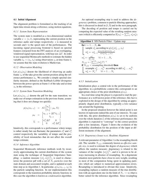
4.1 Initial AlignmentThe alignment problem is formulated as the tracking of aninput data stream along a reference, using motion equations.4.1.1 System State RepresentationThe system state is modeled as a two-dimensional randomvariable x = (s, t), representing the current position in thereference audio and tempo respectively; s is measured inseconds and t is the speed ratio of the performances. Theincoming signal processing frontend is based on spectralfeatures extracted from the FFT analysis of an overlapping,windowed signal representation, with hop size ∆T . In orderto use sequential Montecarlo methods to estimate the hiddenvariable x k = (s k , t k ) using observation z k at time frame k,we assume that the state evolution is Markovian.4.1.2 Observation ModelingLet p(z k |x k ) denote the likelihood of observing an audioframe z k of the take given the current position along the referenceperformance s k . We consider a simple spectral similaritymeasure, defined as the Kullback-Leibler divergencebetween the power spectra at frame k of the take and at times k in the reference.4.1.3 System State Transition ModelingLet p(x k |x k−1 ) denote the pdf for the state transition; wemake use of tempo estimation in the previous frame, assumingthat it does not change too quickly:[ ]skp(x k |x k−1 ) = N ( | µt k , Σ)k[ ]sk−1 + ∆T tµ k =k−1t k−1[ ]σ2Σ = s ∆T 00 σt 2 ∆TIntuitively, this corresponds to a performance where tempois rather steady but can fluctuate; the parameters σ 2 t and σ 2 scontrol respectively the variability of tempo and the possibilityof local mismatches that do not affect the overalltempo estimate.4.1.4 Inference AlgorithmSequential Montecarlo inference methods work by recursivelyapproximating the current distribution of the systemstate using the technique of Sequential Importance Sampling:a random measure {x i k , wi k }Ns i=1is used to characterizethe posterior pdf with a set of N s particles over thestate domain and associated weights, and is updated at eachtime step as in Algorithm 1. In particular, q(x k |x k−1 , z k ) isthe particle sampling function. In our implementation thiscorresponds to the transition probability density function; inthis case the algorithm is known as condensation algorithm.An optional resampling step is used to address the degeneracyproblem, common to particle filtering approaches;this is discussed in detail in [1,5] and in the next paragraph.The decoding of position and tempo is carried out bycomputing the expected value of the resulting random measure(which is efficiently computed as E[x k ] = ∑ N si=1 xi k wi k ).Algorithm 1: SIS Particle Filter - Update stepfor i = 1 . . . N s dosample x i k according to q(xi k |xi k−1 , z k)w i k ←ŵk i ← wi p(z k |x i k )p(xi k |xi k−1 )k−1 q(x i k |xi k−1 ,z k)ŵi k ∑j ŵj k∀i = 1 . . . N sN eff ← ( ∑ N si=1 (wi k )2 ) −1if N eff < resampling threshold thenresample x 1 k . . . xNs kaccording to ddf wk 1 . . . wNs kwk i ← N s−1 ∀i = 1 . . . N s4.1.5 InitializationInitialization plays a central role in the performance of thealgorithm; in a probabilistic context this corresponds to anappropriate choice of the prior distribution p(x 0 ).In a real-time setup the player is expected to start the performanceat a well known point of the reference; this fact isexploited in the design of the algorithm by setting an appropriatelyshaped prior distribution, typically a low-varianceone around the beginning.In the proposed situation however the initial point is notknown (it represents indeed the aim of our interest). To copewith this, the prior distribution p(x 0 ) is set to be uniformover the whole duration L of the reference performance; thealgorithm is expected to “converge” to the correct positionafter a few iterations. Figure 3 shows the evolution of theprobability distribution for the position of the input at differentmoments of the alignment.4.1.6 Degeneracy Issues w.r.t. Realtime AlignmentA relevant parameter of Algorithm 1 is the resampling threshold.The variable N eff , commonly known as effective samplesize, is used to estimate the degree of degeneracy whichaffects the random measure; degeneracy is related to thevariance of the weights {wk i }Ns 1 , and it is proven to be alwaysincreasing in absence of resampling. In a degeneratesituation most particles have close-to-zero weight, resultingin most of the computation being spent in updating particleswhich are subject to numerical approximation errors.Resampling is introduced to obviate this issue. Intuitively,resampling replaces a random measure of the true distributionwith an equivalent one (in the limit of N s → ∞) that isbetter suited for the inference algorithm. Since resampling
Page 1: ACCELERATING THE MIXING PHASE IN ST
Page 5 and 6: the take is then reversed and proce

accelerating the mixing phase in studio recording productions by ...

You also want an ePaper? Increase the reach of your titles

Delete template?

Save as template?