Advances in the Modelling of Motorcycle Dynamics - ResearchGate

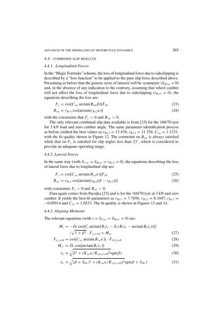
ADVANCES IN THE MODELLING OF MOTORCYCLE DYNAMICS 2654.4. COMBINED SLIP RESULTS4.4.1. Longitudinal ForcesIn the “Magic Formula” scheme, the loss of longitudinal force due to sideslipping isdescribed by a “loss function” to be applied to the pure slip force described above.Presuming as before that the generic tyres of interest will be symmetric (S Hxα = 0)and, in the absence of any indication to the contrary, assuming that wheel camberwill not affect the loss of longitudinal force due to sideslipping (r Bx3 = 0), theequations describing the loss are:F x = cos[C xα arctan(B xα β)]F x0 (23)B xα = r Bx1 cos[arctan(r Bx2 κ)] (24)with the constraints that F x > 0 and B xα > 0.The only relevant combined slip data available is from [23] for the 160/70 tyrefor 3 kN load and zero camber angle. The same parameter identification processas before yielded the best values as r Bx1 = 13.476; r Bx2 = 11.354; C xα = 1.1231,with the fit quality shown in Figure 12. The constraint on B xα is always satisfiedwhile that on F x is satisfied for slip angles less than 23 ◦ , which is considered toprovide an adequate operating range.4.4.2. Lateral ForcesIn the same way (with S Vyκ = S Hyκ = r By4 = 0), the equations describing the lossof lateral force due to longitudinal slip are:F y = cos[C yκ arctan(B yκ κ)]F y0 (25)B yκ = r By1 cos[arctan{r By2 (β − r By3 )}] (26)with constraints F y > 0 and B yk > 0.Data again comes from Pacejka [23] and is for the 160/70 tyre at 3 kN and zerocamber. It yields the best-fit parameters as r By1 = 7.7856, r By2 = 8.1697, r By3 =−0.05914 and C yκ = 1.0533. The fit quality is shown in Figures 13 and 14.4.4.3. Aligning MomentsThe relevant equations (with s = S Vyκ = S Hyκ = 0) are:M z =−D t cos[C t arctan{B t λ t − E t (B t λ t − arctan(B t λ t ))}]/ √ 1 + β 2 · F y,γ =0 + M zr (27)F y,γ =0 = cos[C yκ arctan(B yκ κ)] · F y0,γ =0 (28)M zr = D r cos[arctan(B r λ r )]√(29)λ t = β 2 + (K xκ κ/K yα,γ =0 ) 2 sgn(β) (30)√λ r = (β + S Hr ) 2 + (K xκ κ/K yα,γ =0 ) 2 sgn(β + S Hr ) (31)