


Create successful ePaper yourself
Turn your PDF publications into a flip-book with our unique Google optimized e-Paper software.
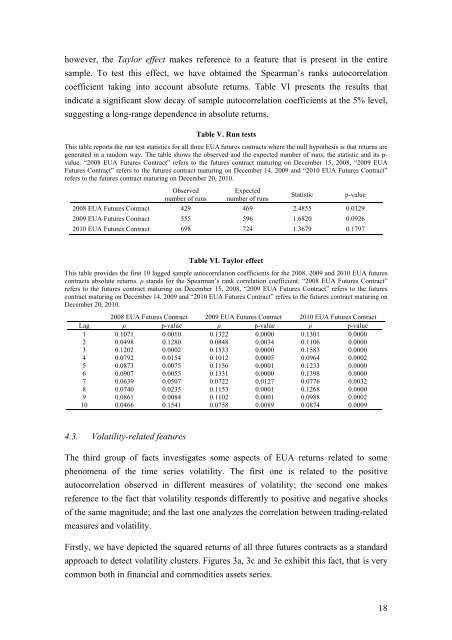
however, the Taylor effect makes reference to a feature that is present in the entire<br />
sample. To test this effect, we have obtained the Spearman’s ranks autocorrelation<br />
coefficient taking into account absolute returns. Table VI presents the results that<br />
indicate a significant slow decay of sample autocorrelation coefficients at the 5% level,<br />
suggesting a long-range dependence in absolute returns.<br />
Table V. Run tests<br />
This table reports the run test statistics for all three EUA futures contracts where the null hypothesis is that returns are<br />
generated in a random way. The table shows the observed and the expected number of runs, the statistic and its p-<br />
value. “2008 EUA Futures Contract” refers to the futures contract maturing on December 15, 2008, “2009 EUA<br />
Futures Contract” refers to the futures contract maturing on December 14, 2009 and “2010 EUA Futures Contract”<br />
refers to the futures contract maturing on December 20, 2010.<br />
Observed<br />
number of runs<br />
Expected<br />
number of runs<br />
Statistic<br />
p-value<br />
2008 EUA Futures Contract 429 469 2.4855 0.0129<br />
2009 EUA Futures Contract 555 596 1.6820 0.0926<br />
2010 EUA Futures Contract 698 724 1.3679 0.1797<br />
Table VI. Taylor effect<br />
This table provides the first 10 lagged sample autocorrelation coefficients for the 2008, 2009 and 2010 EUA futures<br />
contracts absolute returns. ρ stands for the Spearman’s rank correlation coefficient. “2008 EUA Futures Contract”<br />
refers to the futures contract maturing on December 15, 2008, “2009 EUA Futures Contract” refers to the futures<br />
contract maturing on December 14, 2009 and “2010 EUA Futures Contract” refers to the futures contract maturing on<br />
December 20, 2010.<br />
2008 EUA Futures Contract 2009 EUA Futures Contract 2010 EUA Futures Contract<br />
Lag ρ p-value ρ p-value ρ p-value<br />
1 0.1071 0.0010 0.1322 0.0000 0.1301 0.0000<br />
2 0.0498 0.1280 0.0848 0.0034 0.1106 0.0000<br />
3 0.1202 0.0002 0.1533 0.0000 0.1583 0.0000<br />
4 0.0792 0.0154 0.1012 0.0005 0.0964 0.0002<br />
5 0.0873 0.0075 0.1156 0.0001 0.1233 0.0000<br />
6 0.0907 0.0055 0.1331 0.0000 0.1398 0.0000<br />
7 0.0639 0.0507 0.0722 0.0127 0.0776 0.0032<br />
8 0.0740 0.0235 0.1153 0.0001 0.1268 0.0000<br />
9 0.0861 0.0084 0.1102 0.0001 0.0988 0.0002<br />
10 0.0466 0.1541 0.0758 0.0089 0.0874 0.0009<br />
4.3. Volatility-related features<br />
The third group of facts investigates some aspects of EUA returns related to some<br />
phenomena of the time series volatility. The first one is related to the positive<br />
autocorrelation observed in different measures of volatility; the second one makes<br />
reference to the fact that volatility responds differently to positive and negative shocks<br />
of the same magnitude; and the last one analyzes the correlation between trading-related<br />
measures and volatility.<br />
Firstly, we have depicted the squared returns of all three futures contracts as a standard<br />
approach to detect volatility clusters. Figures 3a, 3c and 3e exhibit this fact, that is very<br />
common both in financial and commodities assets series.<br />
18


