JPE - Sept09 - cover2-4.pmd - Pipes & Pipelines International ...

September, 2009 Vol.8, No.3
Scientific
Surveys Ltd, UK
Journal of
Pipeline Engineering
incorporating
The Journal of Pipeline Integrity
Sample issue
Clarion
Technical Publishers, USA

Journal of Pipeline Engineering
Editorial Board - 2009
Obiechina Akpachiogu, Cost Engineering Coordinator, Addax Petroleum
Development Nigeria, Lagos, Nigeria
Mohd Nazmi Ali Napiah, Pipeline Engineer, Petronas Gas, Segamat, Malaysia
Dr Michael Beller, NDT Systems & Services AG, Stutensee, Germany
Jorge Bonnetto, Operations Vice President, TGS, Buenos Aires, Argentina
Mauricio Chequer, Tuboscope Pipeline Services, Mexico City, Mexico
Dr Andrew Cosham, Atkins Boreas, Newcastle upon Tyne, UK
Prof. Rudi Denys, Universiteit Gent – Laboratory Soete, Gent, Belgium
Leigh Fletcher, MIAB Technology Pty Ltd, Bright, Australia
Roger Gomez Boland, Sub-Gerente Control, Transierra SA,
Santa Cruz de la Sierra, Bolivia
Daniel Hamburger, Pipeline Maintenance Manager, El Paso Eastern Pipelines,
Birmingham, AL, USA
Prof. Phil Hopkins, Executive Director, Penspen Ltd, Newcastle upon Tyne, UK
Michael Istre, Engineering Supervisor, Project Consulting Services,
Houston, TX, USA
Dr Shawn Kenny, Memorial University of Newfoundland – Faculty of Engineering
and Applied Science, St John’s, Canada
Dr Gerhard Knauf, Mannesmann Forschungsinstitut GmbH, Duisburg, Germany
Lino Moreira, General Manager – Development and Technology Innovation,
Petrobras Transporte SA, Rio de Janeiro, Brazil
Prof. Andrew Palmer, Dept of Civil Engineering – National University of Singapore,
Singapore
Prof. Dimitri Pavlou, Professor of Mechanical Engineering,
Technological Institute of Halkida , Halkida, Greece
Sample issue
Dr Julia Race, School of Marine Sciences – University of Newcastle,
Newcastle upon Tyne, UK
Dr John Smart, John Smart & Associates, Houston, TX, USA
Jan Spiekhout, NV Nederlandse Gasunie, Groningen, Netherlands
Dr Nobuhisa Suzuki, JFE R&D Corporation, Kawasaki, Japan
Prof. Sviatoslav Timashev, Russian Academy of Sciences – Science
& Engineering Centre, Ekaterinburg, Russia
Patrick Vieth, Senior Vice President – Integrity & Materials,
CC Technologies, Dublin, OH, USA
Dr Joe Zhou, Technology Leader, TransCanada PipeLines Ltd, Calgary, Canada
Dr Xian-Kui Zhu, Senior Research Scientist, Battelle Pipeline Technology Center,
Columbus, OH, USA
❖ ❖ ❖

3rd Quarter, 2009 145
The Journal of
Pipeline Engineering
incorporating
The Journal of Pipeline Integrity
Volume 8, No 3 • Third Quarter, 2009
Contents
Dr Mohamad J Cheaitani ....................................................................................................................................... 149
Approaches for determining limit load and reference stress for circumferential embedded flaws in pipe girth welds
Nigel S Kirk and Dipl-Ing Björn Dobberstein...................................................................................................... 167
The Nord Stream Pipeline’s German landfall: the challenges ahead
Dr Kimberly Cameron and Dr Alfred Pettinger .................................................................................................. 175
Assessing pipeline integrity using fracture mechanics and currently available inspection tools
Navid Nazemi, Sara Kenno, and Sreekanta Das ................................................................................................... 183
Behaviour of wrinkled linepipe subjected to internal pressure and eccentric axial compression load
Kenton Pike ............................................................................................................................................................ 191
Advanced numerical modelling tools aid Arctic pipeline design
Sample issue
Etim S Udoetok and Anh N Nguyen .................................................................................................................... 195
A disc pig model for estimating the mixing volumes between product batches in multi-product pipelines
J P Pruiksma, H J Brink, H M G Kruse, and J Spiekhout .................................................................................. 205
Soil reaction force at the head of the pipeline during the pull-back operation of horizontal directional drilling
Stijn Hertelé, Rudi Denys, and Wim De Waele................................................................................................... 213
Full range stress-strain relation modelling of pipeline steels
Correction ............................................................................................................................................................... 223
A practical approach to pipeline corrosion modelling: Part 2 – Short-term integrity forecasting
❖ ❖ ❖
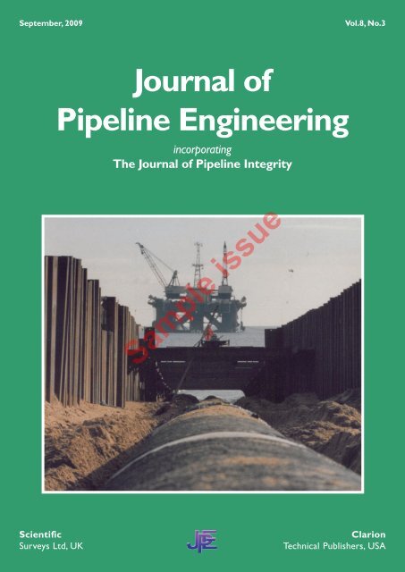
OUR COVER PICTURE shows a typical landfall using a coffer dam to pull-in the pipe from offshore, one of the
techniques being proposed by the designers of the Nord Stream pipeline project. The twin 48-in diameter, 1220-km
long, pipelines will be the world’s longest subsea pipelines once fully operational in 2011. The first of a series of
three papers describing aspects of the project is published on pages 167-173.

146
1. Disclaimer: While every effort is made to check the
accuracy of the contributions published in The Journal of
Pipeline Engineering, Scientific Surveys Ltd and Clarion
Technical Publishers do not accept responsibility for the
views expressed which, although made in good faith, are
those of the authors alone.
2. Copyright and photocopying: © 2009 Scientific Surveys
Ltd and Clarion Technical Publishers. All rights reserved.
No part of this publication may be reproduced, stored or
transmitted in any form or by any means without the prior
permission in writing from the copyright holder.
Authorization to photocopy items for internal and personal
use is granted by the copyright holder for libraries and
other users registered with their local reproduction rights
organization. This consent does not extend to other kinds
of copying such as copying for general distribution, for
advertising and promotional purposes, for creating new
collective works, or for resale. Special requests should be
addressed to Scientific Surveys Ltd, PO Box 21, Beaconsfield
HP9 1NS, UK, email: info@scientificsurveys.com.
3. Information for subscribers: The Journal of Pipeline
Engineering (incorporating the Journal of Pipeline Integrity)
is published four times each year. The subscription price
for 2009 is US$350 per year (inc. airmail postage). Members
of the Professional Institute of Pipeline Engineers can
subscribe for the special rate of US$175/year (inc. airmail
postage). Subscribers receive free on-line access to all issues
of the Journal during the period of their subscription.
The Journal of Pipeline Engineering
THE Journal of Pipeline Engineering (incorporating the Journal of Pipeline Integrity) is an independent, international,
quarterly journal, devoted to the subject of promoting the science of pipeline engineering – and maintaining and
improving pipeline integrity – for oil, gas, and products pipelines. The editorial content is original papers on all aspects
of the subject. Papers sent to the Journal should not be submitted elsewhere while under editorial consideration.
Authors wishing to submit papers should send them to the Editor, The Journal of Pipeline Engineering, PO Box 21,
Beaconsfield, HP9 1NS, UK or to Clarion Technical Publishers, 3401 Louisiana, Suite 255, Houston, TX 77002, USA.
Instructions for authors are available on request: please contact the Editor at the address given below. All contributions
will be reviewed for technical content and general presentation.
The Journal of Pipeline Engineering aims to publish papers of quality within six months of manuscript acceptance.
Notes
4. Back issues: Single issues from current and past volumes
(and recent issues of the Journal of Pipeline Integrity) are
available for US$87.50 per copy.
5. Publisher: The Journal of Pipeline Engineering is
published by Scientific Surveys Ltd (UK) and Clarion
Technical Publishers (USA):
Scientific Surveys Ltd, PO Box 21, Beaconsfield
HP9 1NS, UK
tel: +44 (0)1494 675139
fax: +44 (0)1494 670155
email: info@scientificsurveys.com
web: www.j-pipe-eng.com
www.pipemag.com
Editor and publisher: John Tiratsoo
email: jtiratsoo@j-pipe-eng.com
Sample issue
v v v
Clarion Technical Publishers, 3401 Louisiana,
Suite 255, Houston TX 77002, USA
tel: +1 713 521 5929
fax: +1 713 521 9255
web: www.clarion.org
Associate publisher: BJ Lowe
email: bjlowe@clarion.org
6. ISSN 1753 2116
www.j-pipe-eng.com
is available for subscribers

3rd Quarter, 2009 147
Editorial
Pipeline outlook: it’s not all gloom
FOR A CONSIDERABLE time, headlines around the
world have been focussing on the economic situation
and the immense difficulties the downturn has imposed on
individuals and companies in many industrial sectors.
There is no denying the fact that huge changes are under
way, and the world as a whole is having to readjust to the
new regime that these changes are introducing. Many
might therefore see this as a poor choice of time at which
to launch a new industry publication. The hydrocarbons’
pipeline industry is, however, particularly buoyant currently,
and forecasts for the next five years are tremendously
positive for both on- and offshore pipeline construction.
Fuelled, of course, by the world’s burgeoning need for
energy, gas pipeline projects have never been of greater
significance, and are focussing on transporting reserves
from more technically-challenging areas than ever before.
Oil, too, is in high demand, and requires transport over
longer distances and through terrain of increasing
complexity and environmental sensitivity.
Two recently-published authoritative reports highlight the
strength of the pipeline industry and its forecast growth
over the next few years. Looking offshore, London-based
Infield Energy Analysts’ fourth edition of its Global
perspectives pipelines and control lines update report provides
an in-depth, independent analysis of the global offshore
pipeline and control line market sectors from 2004 to
2013. The report covers pipelines of all lengths and diameters
including SURF flowlines, trunklines, and conventional
pipelines, as well as all control lines, including
communication, power line, seismic cable,
telecommunication, and umbilicals.
With the long-term prospect of increasing global energy
demand, securing future energy supplies has become a
common global issue. As the report points out, for those
countries with dwindling production rates or low
hydrocarbon reserves, the pressure for energy security is set
to increase, while those with abundant reserves will strive
to attract investment to enable adequate development to
meet both domestic and foreign energy demands. As a
consequence of these demands, there has been growth in
the offshore oil and gas industry since 2004. A lower price
outlook and lack of available credit have certainly affected
the future development of reserves, but growth in the
industry is still expected to continue.
Pipeline and control line installation trends have mirrored
those of the wider offshore industry, which is unsurprising,
considering their crucial role within the offshore oil and
gas infrastructure, and Infield forecasts the total pipelines
and control lines capital expenditure to exceed $265bn
over the period 2009-2013. This equates to 103,435km of
lines being installed, of which 81,293km will be pipelines
and 22,142km will be control lines. Combined, these
represent an increase of 68% in installations over that’s of
the previous five years. The forecasted increase will be
dominated by growth in the pipeline market, with a
significantly-slower growth in the control line market. A
considerable percentage of the forecast pipeline expenditure
is related to far-advanced trunklines, many un-connected to
specific field development projects and, as such, key
infrastructure development.
Sample issue
Infield says that the next five years indicate a change in
market demographics, in which all pipeline segments will
hold fairly equal shares of the installation market. This
follows a period in which conventional pipelines dominated
the installation market, highlighting the industry’s
historically-favoured shallow-water developments. However,
as shallow-water production rates fall, the industry has
sought to discover and develop deeper-water reserves. As a
consequence, subsea construction, umbilical, riser, and
flowline (SURF) installations have grown in the previous
five-year period, and are set to continue increasing in the
forecast period. The largest pipeline installation growth is
expected in the trunk/export lines sector, further
characterizing the increasing demand to secure a diversified
mix of future energy supplies.
Whilst growth is still expected in the control line market,
a decline in communication line installations and slower
growth in the power line sector will be seen compared to
the previous five-year period. The overall control line
growth will predominantly be driven by an increase in
umbilical and bundled pipeline installations, both of which

148
imply the continuing trend to replace installation of single
control lines with combined multiple line installations.
Overall however, as the report highlights, the future for the
pipeline and control line industry is expected to be strong
with a variety of water depths, project sizes, and locations
expected over the next five years.
As far as the onshore industry is concerned, Douglas-
Westwood’s report points out that around 157,000km of
pipelines are planned up to 2013, at a cost of over $178
billion, which is a 15% increase in length installed and a
27% increase in investment relative to the previous fiveyear
period. Gas pipelines will make up 95,341km, and oil
pipelines 35,034km, of the total, in which LNG
transportation will also play a significant role. Some specific
projects that will contribute to these totals are featured in
this issue, among which are reviews of various aspects of the
twin 1220-km long, 48-in diameter, Nord Stream pipelines,
which will be the longest subsea pipelines in the world
when commissioned in 2011 and 2012. The issues
surrounding the design and engineering of pipelines in the
Arctic, a region that is becoming of great significance, are
also becoming increasingly high-profile. As a testament to
this, the proposed pipeline to bring Alaskan gas to markets
in the southern United States is expected to cost over $30
billion, and the latest published cost estimate for the
Mackenzie gas pipeline from the Mackenzie Delta area is
$16 billion.
Publishers merge: new industry
magazine launched
TWO OF THE LEADING providers of technical and
business information for the pipeline industry,
Scientific Surveys Ltd and Great Southern Press (GSP),
have merged. The newly formed company has a global
The Journal of Pipeline Engineering
scope, with head offices in the UK and the Asia Pacific, as
well as a strong presence in Houston and contacts
throughout South America, Europe and the Middle East.
The companies will, together, continue to produce their
full range of pipeline products, and have already launched
a new print magazine, Pipelines International, which is
supported by a comprehensive online presence (see
www.pipelinesinternational.com) and will reflect the
diversity of the pipeline industry world-wide. As part of the
merger, the new business division will – in association with
Clarion of Houston – continue publication of the Journal
of Pipeline Engineering, along with developing the
comprehensive database of technical papers at
www.pipedata.com, and expanding its involvement with
high-quality training courses and events.
Formation of the new division is intended to build-upon
the reputations of UK-based Scientific Surveys and
Australian GSP in providing technical information, and
the strong partnership with Clarion in Houston will be
developed and enhanced. In addition to the world-renowned
Pipeline Pigging & Integrity Management Conference and
Exhibition in Houston each February, new major
conferences and exhibitions, as well as training, will be
planned elsewhere, including in the Asia-Pacific and Middle
Eastern regions. The partnership will also strengthen the
companies’ other existing products, for example by providing
greater resources and technical expertise to The Australian
Pipeliner magazine.
Sample issue

3rd Quarter, 2009 149
Approaches for determining
limit load and reference stress
for circumferential embedded
flaws in pipe girth welds
by Dr Mohamad J Cheaitani
TWI Ltd, Abington, Cambridge, UK
THIS PAPER PROVIDES an evaluation of approaches for determining limit load (and equivalent reference
stress) for use in failure-assessment diagram (FAD)-based fracture assessment of circumferential
embedded flaws in pipe girth welds. Three-dimensional elastic plastic finite-element analyses have been
conducted on pipe models containing typical circumferential embedded flaws and subject to global bending
loads. ‘J-based’ limit loads (and equivalent reference stresses) and global collapse limit loads have been
determined from the finite-element analyses and used to evaluate existing standard flat-plate solutions,
including those in BS 7910 and R6. A general approach for determining the limit load (and the equivalent
reference stress) is presented. This approach is consistent with both the finite-element results and
reference stress J-estimation scheme and, consequently, allows the development of improved assessment
models.
THE USE OF AN engineering critical assessment (ECA)
to derive flaw acceptance criteria for pipeline girth
welds allows the maximum tolerable size of surface and
embedded circumferential planar flaws to be determined
on a fitness-for-purpose basis. A typical ECA involves
assessing the significance of such flaws with regard to
failure mechanisms, including fracture, which the pipeline
may experience during construction, commissioning, and
service. The most commonly used approach to assess the
significance of flaws with regard to fracture and plastic
collapse is the failure-assessment diagram (FAD), which is
based on the reference stress J-estimation scheme [1, 2] . An
FAD-based assessment involves the calculation of a fracture
parameter (K r , d r , or J r ) and a plastic collapse parameter,
This paper was presented at the Pipeline Technology Conference held
in Ostend, Belgium, on 12-14 October, 2009, and organized by the
University of Gent, Belgium, and Technologisch Instituut vzw, Antwerp,
Belgium.
Author’s contact details:
tel: +44 (0)1223 899000
email: mohamad.cheaitani@twi.co.uk
Sample issue
L r , Fig.1. The fracture parameter characterizes the proximity
to fracture under linear elastic conditions. The plasticcollapse
parameter characterizes the proximity to failure by
yielding mechanisms and is defined as either the ratio of
applied load to the limit load or, equivalently, the ratio of
the reference stress to the yield stress. There is a unique
relationship between a reference stress and a limit load
which enables one to be defined if the other is known:
specifically, a limit load is inversely proportional to the
corresponding reference stress as follows:
Applied load Reference stress
=
Limit load Yield stress
The work described in this paper concerns the development
of a reference-stress (or limit-load) model for use in FADbased
fracture assessments of circumferential embedded
girth weld flaws such as that shown in Fig.2. This work is
considered necessary since existing reference-stress solutions
for embedded flaws are not consistent with the referencestress
solutions that are typically used to assess surface
(1)

150
K r (fracture parameter)
1.2
1
0.8
0.6
0.4
0.2
flaws, because the approaches used in their derivation are
different. Whereas there are several reference-stress models
for surface-breaking flaws, including some intended
specifically for circumferential flaws in pipe sections, there
are fewer reference-stress models for embedded flaws, and
these are intended for flaws in flat plates.
One of the most widely used solutions is that in BS
7910:2005 [1], which assumes that plastic collapse occurs
locally when the net section stress on a small area
surrounding the embedded flaw reaches the yield or flow
strength of the material. It also assumes that tensile loads
are applied through a pin-jointed coupling, i.e. that there
is negligible bending restraint. The use of this solution to
assess embedded flaws could lead to overly conservative
results, which may in some cases be counter-intuitive: for
example, for a given applied loading, the maximum tolerable
length for an embedded flaw (whose ligament is greater
than or equal to the height of one weld pass) is smaller than
that for a surface-breaking flaw of the same height.
The paper focuses on the evaluation of the existing referencestress
(and the equivalent limit-load) solutions for embedded
flaws and the development of improved models. The existing
solutions are evaluated using data generated from elasticplastic
finite-element analyses of pipe models containing
typical circumferential embedded flaws.
Scope of work
Acceptable
Not acceptable
0
0 0.2 0.4 0.6 0.8 1 1.2
L r (yielding or collapse parameter)
The scope of work includes three-dimensional elastic-plastic
finite-element analyses of pipe models containing typical
circumferential embedded flaws. The pipe models were
loaded by pure bending, which is the pre-dominant loading
mode during pipeline installation, and were perfectly aligned
across the section containing the flaw; the same tensile
properties were assigned to the parent and weld metals.
Data from the finite-element analyses were used to review
and evaluate a number of methods for determination of the
reference stress (or limit load) for embedded flaws, including
the conventional methods recommended in BS 7910 [1]
The Journal of Pipeline Engineering
and R6 [2], and novel methods. It is shown that none of the
existing codified reference-stress (or limit-load) solutions
agree well with the results obtained from the finite-element
analyses. Therefore, a new approach using a novel method
for definition of reference stress, which is fully consistent
with the findings from the finite-element analyses, is
proposed.
The remainder of this paper consists of the following
sections: reference stress J-estimation scheme; approaches
for determining reference stresses (and limit loads) in FADbased
assessments; codified reference-stress (and limit-load)
solutions for embedded flaws; approach adopted for
determining J-based limit loads (M J ); scope of (and results
from) finite-element analyses; comments on global collapse
and J-based limit loads; comparison of flat-plate solutions
with J-based solutions; plastic strain in ligaments; and
summary and conclusions.
Sample issue
Reference stress
J-estimation scheme
The evaluation of reference-stress models is performed
within the context of the reference stress J-estimation
scheme [2], which is defined below.
J is estimated from the following expressions, which
correspond to the material-specific FAD (BS 7910 Level
2B/3B and R6 Option 2):
Je
J = 2
fL ( )
(2)
and
r
3
−0.5
⎛Eεref Lrσ
⎞
y ⎟
f( Lr
) =
⎜ ⎟
⎜ + ⎟
⎜⎝Lrσy2Eε ⎟ ref ⎠
Fig.1. A typical failure-assessment
diagram (FAD).
where, for a given applied bending moment, M:
(3)

3rd Quarter, 2009 151
L r s y is the reference stress (denoted as s ref );
e ref is the reference strain corresponding to s ref and
determined from the stress-strain curve of the
material;
s y is the yield or 0.2% proof strength of the material;
and
E is Young’s modulus.
J e is the elastic value of J at an applied moment M,
determined from data obtained at an applied moment M o ,
as follows:
⎛ M ⎞
= ⎜
⎟
⎜⎜⎝ ⎟
⎠⎟
Je Jo Mo
2
or using the equivalent expression
where:
2
⎛ ⎞
M
e = ⎜ ⎟
o⎜⎟
⎜⎜⎝σ ⎟
o ⎠
J J σ
J o is the elastic value of J determined at M o (for example,
from an elastic finite-element analysis); and
s M and s o are the elastic bending stresses on the pipe
OD corresponding to M and M o , respectively,
determined using elastic section properties.
An alternative estimate of the elastic value of J may be
determined as follows:
2
⎛ ⎞
M1
e = ⎜ ⎟
o⎜⎟
⎜⎜⎝ σ
⎟
o ⎠
J J σ
which is similar to Equn 5 but uses the actual elastic-plastic
stress on the pipe OD (denoted s ), rather than s . In this
M1 M
case, J is not proportional to M e 2 .
The parameter L r , which characterizes the proximity to
plastic collapse, can be expressed as follows:
Lr ML
(4)
(5)
(6)
M
= (7)
or alternatively as:
σref
Lr
= (8)
σy
where M is the limit load.
L
The reference stress J-estimation scheme could also be
applied using alternative expressions of J, such as that
which corresponds to simplified FADs in BS 7910 and R6.
There are a number of approaches for determining M L (and
Fig.2. Idealized curved elliptical embedded flaw in a pipe
(located at 12 o’clock position).
the corresponding s ref ), which are described in the following
sections.
Approaches for determining
limit loads for FAD assessments
The limit load (or plastic collapse) required for the
calculation of reference stress and the parameter L r is one
of the most important elements of an FAD-based assessment
since it serves two functions:
• it ensures that the limit load of the component
containing the flaw under consideration is not
exceeded;
• it ensures that the relationship between elasticplastic
driving force and proximity to plastic collapse
is consistent with the relationship implied by the
failure-assessment curve.
Sample issue
Two potential plastic-collapse modes of a flawed component
can be identified:
• Local collapse: corresponds to failure, by yielding
mechanisms, of the ligament adjacent to the flaw.
This is deemed to occur when the stress in the
remaining ligament reaches the yield strength of the
material. With regard to a circumferential partthickness
flaw in a girth weld (surface-breaking or
embedded), the significance of the circumferential
extent of the remaining ligament on either side of
the flaw is not well defined in any of the existing
standards. Another source of uncertainty is whether
bending of the section containing the flaw is
restrained or not. In the absence of bending restraint,
secondary bending stresses arise due to eccentric
loading. This is caused by movement of the neutral

152
axis, due to the existence of the flaw, compared with
the unflawed condition.
• Global collapse: corresponds to failure, by yielding
mechanisms, of the whole section containing the
flaw. This is deemed to occur when the global
deformation, displacement and/or rotation, of the
section become unbounded. Global collapse occurs
at a higher load than that corresponding to local
collapse.
Most codified limit-load or reference-stress solutions for
part-thickness (surface or embedded) flaws are based on the
local-collapse approach. Although some standards, such as
R6 [2] also provide solutions based on the global-collapse
approach, further checks, such as against finite-element
analyses, may be required to verify that such solutions
provide safe assessments.
An alternative method for determining limit loads, which
requires J data from finite-element analyses, consists of
defining the limit load such that it is consistent with the J
data and the reference stress J-estimation scheme represented
by Equn 2. The main benefit of this approach is that it does
not require the analyst to specify in advance whether a localor
global-collapse model is more suitable. The limit load is
found by solving Equns 2 and 3 using J results from an
elastic-plastic finite-element analysis of the flawed
component. A simple version of this approach is
recommended in Section B.6.4.3(e) of API 579 [3] and in
a slightly different form in Section B.1.89 of API-579-1/
ASME-FFS-1 [4] as follows:
L
r
t
Fig.3. Idealized elliptical embedded flaw in a flat plate, used in BS 7910 (BSI, 2005).
P
=
P
ref
where P ref is determined from the following relationship:
(9)
The Journal of Pipeline Engineering
J 0.002E 1 ⎛ 0.002E⎞
⎟
= 1+ +
⎜
⎜1
⎟
Je σy 2
⎜ + ⎟
⎜⎝ σ ⎟ y ⎠
P= Pref
−1
(10)
where J is the total value of J determined from an elasticplastic
analysis of the flawed component; J e is the elastic J
determined from an elastic analysis by, for example, using
Equns 4 or 5; P is a characteristic applied load (or stress)
such as axial force, bending moment, or a combination
thereof; and P ref is the reference load (or stress) defined as
the load at which the ratio J/J e reaches the value defined by
Equn 10.
If P ref is used to construct a BS 7910 Level 3C FAD (with L r
defined according to Equn 9), it will intersect the
corresponding BS 7910 Level 2B/3B material-specific FAD,
and give the same K r value, at L r = 1.0. Thus, the limit load
P ref is defined in a manner which is consistent with the Level
2B/3B material-specific FAD, at least at L r = 1.0. In this
case, the limit load may depend on the strain-hardening
characteristics of the material.
Sample issue
Codified reference-stress
solutions for embedded flaws
General
Whereas there are several well-established reference-stress
solutions for circumferential surface flaws in pipe girth
welds, there are no such solutions for circumferential
embedded flaws. Consequently, most analysts use referencestress
solutions originally derived for flat plates to assess
circumferential embedded flaws in pipe girth welds. The
most widely used of these solutions are the reference-stress
equations given in BS 7910 [1] and R6 [2]. These are given
in terms of the membrane stress, P m , and through-wall

3rd Quarter, 2009 153
Fig.4. Idealized
rectangular embedded
flaw in a flat plate
subjected to tension
and/or bending loading,
used in R6 (BEGL,
2001).
bending stress, P b . However, given that in a thin-walled
pipe loaded by bending P b is very small compared with P m ,
and in a pipe loaded by tension P b is equal to zero, the
reference-stress equations considered below are given
assuming that P b is equal to zero. Note that references to
equations, sections, and figures in codes and standards are
shown in italics.
BS 7910
The embedded flaw reference stress equation in Equation
P4 of BS 7910 [1] is based on local collapse and assumes
that tensile loads are applied through pin-jointed coupling,
i.e. that there is negligible bending restraint. The equation
was derived by Willoughby and Davey [5] assuming that the
load-bearing area (or ligament) extends to the plate surfaces
above and below the embedded flaw and has a length equal
to the flaw length plus one plate thickness on either end of
the flaw. The solution, with P b set at zero, is as follows:
σ
ref
{ }
⎡ 2 2
2 4 α"
p ⎤
Pmα" + ⎢( Pmα" ) + Pm
( 1 − α"
) + ⎥
⎢ t ⎥
= ⎣ ⎦
2 4 α"
p
( 1 − α"
) +
t
0.5
(11)
where p is the ligament (the smallest distance between the
flaw and the surface), t is the wall thickness, and
2a
α " =
⎛ t ⎞⎟
t ⎜
⎜⎜⎝ 1+
⎟
c⎠⎟
(12)
where 2a is the flaw height and 2c is its length – see Fig.3
(note that the wall thickness in BS 7910 is denoted as B).
R6
R6 [2] provides several reference stress solutions for
embedded flaws in flat plates, which are based on local or
global collapse with loads applied through pin-jointed
coupling (i.e. pin loading) or fixed-grip loading conditions.
The approach used to develop these solutions is described
by Lei and Budden [6]. The solutions cater for flaws located
fully or partially in the tensile stress zone (determined by
the location of the neutral axis). Whilst this distinction is
important when assessing flat plates, it is less significant for
circumferential embedded flaws in pipe girth welds, which
are almost always assumed to be in the tensile stress zone.
Consequently, attention is focussed below on the latter
condition. The solutions are expressed using the following
parameters:
N a c
n
Wt t W k
y
L
off c
L = , a= , b = , = , g =
2 s t t
Sample issue
y
where N L is the limit load and other parameters are illustrated
in Fig.4. The limit-load solutions are given below in terms
of the non-dimensional parameter n L .
Global collapse, pin-loaded (IV.1.6.3-1):
c1
nL
=
2
2ab + 4(
ab)
+ c
1
(IV.1.6.1-1 with l = 0) (13)
2
c = 1-8abk-4( ab)
(IV.1.6.1-3) (14)
1
Valid for:
1
1
> k³ 0 anda£ -k
2
2

154
Stress (MPa)
Global collapse, fixed-grip tension (IV.1.6.3-1 with k = 0):
As above (Equns 13 and 14) but with k = 0 (the limit load
does not depend on the crack position in the cross section).
Local collapse, pin-loaded (IV.1.6.3.2), solution (a):
d= t+ c, t1= t and W > d
This solution is approached when yielding takes place
across the whole loading-bearing area 2(t + c) t.
n
L
600
500
400
300
200
100
Stress (MPa)
0
0 1 2 3 4 5 6 7 8 9 10
400
300
200
100
=
⎛ αγ ⎞
2 ⎜
⎟ ⎟+ ⎜⎝1+ γ
⎟ ⎟⎠ c1
2
⎛ αγ ⎞
4 ⎜
⎟ + c
⎜
1
⎝1+ γ⎠
⎟
(IV.1.6.2-1 with l = 0) (15)
2
Strain %
8αγ
k ⎛ αγ⎞
c1
= 1− −⎜
⎜ ⎟
1 γ ⎜1 γ
⎟ (IV.1.6.2-3) (16)
+ ⎜⎝
+ ⎠ ⎟
Valid for:
1
1
g
> k ³ 0 and a£ - k and b<
2
2 1+
g
True stress R-O n=15
Eng stress R-O n=15
0.2% offset
0
0 0.2 0.4 0.6 0.8
Strain %
The Journal of Pipeline Engineering
True stress R-O n=15
Eng stress R-O n=15
0.2% offset Fig.5. Stress-strain curve used:
Local collapse, pin-loaded (IV.1.6.3.2), solution (b):
d= t+ c, t1= t and W > d
Sample issue
This is approached when yielding spreads through the
smallest ligament along the plate thickness. Solution (b) is
always less than or equal to Solution (a).
⎛ 2α
⎞
d= t ⎜
⎜1 ⎟
⎜⎝
− ⎟+
c, t1= t( 1− 2k)
and W > d
1−2k⎠⎟ n
L
⎛ 2α
⎞
⎜
⎜1 ⎟
⎜⎝
− ⎟(
1+
γ)
1−2k⎠⎟ =
⎛ 2α
⎞⎟
⎜
⎜⎜⎝ 1− ⎟+
γ
1−2k⎟⎠ Local collapse, fixed-grip tension:
1+ g( 1-2a) nL =
1+
g
(a - top) curve up to 10% strain;
(b - bottom) curve up to 0.8% strain.
(17)
(18)
(19)

3rd Quarter, 2009 155
Approach adopted for determining
J-based limit loads (M J )
As evident from the above, there are numerous approaches
for the definition of limit load including local collapse,
global collapse, or J-based methods associated with the
reference stress J-estimation scheme. Each of these
approaches can be applied using a number of options. For
example, local collapse can be defined based on a somewhat
arbitrarily postulated load-bearing area, and either fixedended
or pin-ended supports (reflecting whether bending
of the section containing the flaw is restrained or not). In
practice it is difficult to assess the suitability of these
solutions for use in specific applications without additional
information.
The suitability of the above approaches to assess
circumferential embedded flaws in pipe girth welds is
evaluated in the following sections using data from elasticplastic
finite-element analyses of pipe models containing
typical circumferential embedded flaws. A reference stress
(or limit load) is deemed to be adequate if it allows the
effective elastic-plastic crack driving force expressed in
terms of J integral (or J), to be determined using the FADbased
reference stress J-estimation scheme, with a reasonable
degree of accuracy compared to finite-element results.
Therefore, the meaning of the term ‘limit load’ is extended
to include any load that is used to define the reference stress
in the context of a FAD calculation. Within this framework,
the above approaches are assessed against a J-based limit
load, which for a pipe subjected to bending is referred to as
M J . This is determined using an approach somewhat similar
to that of API-579-1/ASME-FFS-1 in that the limit load is
defined to ensure consistency between the Level 3C FAD
and the Level 2B/3B material-specific FAD (Equn 3).
However, unlike the API 579 model which achieves this
consistency at L r = 1.0, M J is determined such that the Level
3C FAD matches the Level 2B/3B FAD at a range of L r and
applied strain values. For each model, M J is determined for
each load increment (in the finite-element analysis) as
follows:
• L r is determined by solving Equns [2] and [3]
• M J is determined as M/L r (according to Equn 7),
where M is the applied moment.
This approach allows M J to be determined for every load
increment and, consequently, allows M J to be plotted as a
function of any loading parameter, including applied
moment, remote applied stress/strain or L r .
In theory, M J may depend on the position along the crack
front. In the present work, attention has been restricted to
solutions in the centre of the crack, which is usually the
position of maximum J.
Finite-element analyses
Three-dimensional elastic-plastic finite-element analyses
were conducted on pipe models containing a range of
embedded flaw geometries. Four pipe geometries with pipe
radius to thickness ratios in the range 5 to 20 were
considered: in this paper, only results from Series E1 (pipe
outside diameter = 400mm, wall thickness = 20mm), which
were conducted using the stress-strain curve shown in Figs
5a and 5b, are reported. The stress-strain curve was
constructed from the following Ramberg-Osgood powerlaw
hardening relationship:
⎛ n
⎛ ⎞ ⎞
Y ⎜ α⎜
⎟ ⎟
⎜ ⎜ ⎟
E σY σ
⎟ ⎟
⎜⎝
⎜ ⎜ ⎜⎝ ⎟
Y ⎠ ⎠ ⎟
σ σ σ
e=
+ ⎟
where:
e = true strain
s = true stress
s Y = 0.2% proof strength (= 400MPa)
E = Young’s modulus (200,000MPa)
n = strain-hardening exponent (= 15)
a = 0.002/e Y (= 1.0)
e Y = s Y /E
(20)
Each finite-element model contained an elliptical embedded
flaw oriented in the circumferential direction and contained
within a plane perpendicular to the pipe axis. The flaws
considered had a height in the range 3 to 9mm, were
located at 1.5 to 14mm from the pipe inside surface, and
had a length, along the ellipse major axis, in the range 25
to 250mm. The flaws were located at the 12 o’clock
position to ensure that they were subjected to the largest
tensile stresses when the model was loaded by bending. The
models were loaded by pure bending, which is the
predominant loading mode during pipeline installation. In
all models, the pipes were perfectly aligned across the
section containing the flaw and the same tensile properties
were assigned to the finite elements representing parent
and weld metals. The dimensions of the pipes and flaws
considered within Series E1 are summarized in Table 1.
Sample issue
All the analyses were performed using ABAQUS Version
6.6 [7] using a small strain formulation, which is considered
to be acceptable at least up to applied strains in the range
0.5 to 1%. The finite-element meshes consist entirely of
type C3D20R elements, which are 20-noded, quadratic,
three-dimensional elements. As the flaw in the pipe is
symmetric about the vertical plane and the applied load is
also symmetric about this plane, it is only necessary to
model half the pipe.
In addition to analyses using the above-mentioned stressstrain
model, analyses were performed on a number of pipe
models using an elastic-perfectly plastic stress-strain model
to determine a global collapse limit load, denoted M FEA .

156
Results
J-based limit loads -
dependence on applied load
Analyses using the above stress-strain model enabled the Jintegral
to be calculated as a function of the applied load
along the crack front. The highest J values, which generally
occurred at the middle of the crack front adjacent to the
smaller of the two ligaments (below and above the flaw),
were adopted.
The Journal of Pipeline Engineering
Pipe dimension
s,
mm
Flaw
dimension
s,
mm
Outside
diameter
Wall
thickne
ss
Height Length
Ligame
nt
to
ID
Ligame
nt
OD
E1BH3L50L1. 5M0
400 20 3 50 1. 5 15.
5
E1BH3L50L3M0400 20 3 50 3 14
E1BH3L50L14M0400 20 3 50 14 3
E1BH3L50L6M0400 20 3 50 6 11
E1BH3L50L9M0400 20 3 50 9 8
E1BH6L50L3M0400 20 6 50 3 11
E1BH6L50L11M0400 20 6 50 11 3
E1BH9L50L3M0400 20 9 50 3 8
E1BH6L50L6M0400 20 6 50 6 8
E1BH6L50L1. 5M0
400 20 6 50 1. 5 12.
5
E1BH3L25L3M0400 20 3 25 3 14
E1BH3L100L3M0400 20 3 100 3 14
E1BH3L200L3M0400 20 3 200 3 14
E1BH3L250L3M0400 20 3 250 3 14
Sample issue
E1BH6L25L3M0400 20 6 25 3 11
E1BH6L100L3M0400 20 6 100 3 11
E1BH3L25L6M0400 20 3 25 6 11
Table 1. Dimensions of pipe and flaw considered in finite-element analysis models (series E1).
The J results were used to estimate the following J-based
limit loads according to the approach described earlier:
• M J2B E – consistent with Equn 2, representing the
material-specific FAD of BS 7910 (Level 2B/3B)
and R6 (Option 2) with J e estimated using the elastic
pipe bending stress according to Equn 5.
• M J2B EP – consistent with Equn 2, representing the
material-specific FAD of BS 7910 (Level 2B/3B)
and R6 (Option 2) with J e estimated using the
elastic-plastic pipe bending stress in Equn 6.
to

3rd Quarter, 2009 157
The above results are shown in Figs 6 and 7 in terms of
2 M /4ts R vs Lr and applied strain, respectively. Here,
J2B EP y m
t is the pipe thickness, R is the pipe mean radius, and s m y
2 is the pipe yield strength. Plots of M /4ts R vs Lr and
J2B E y m
applied strain are not included since they have broadly
similar shapes to those shown in Figs 6 and 7 (but M is J2B E
approximately 4% higher than M ). J2B EP
2 Fig.6. M /4tv R (Je based on elastic-plastic pipe bending stress) vs L .
J2B EP y m
r
Sample issue
2 Fig.7. M /4ts R (Je based on elastic-plastic pipe bending stress) vs remote strain (%).
J2B EP y m
Figures 6 and 7 indicate that M J2B EP increase slightly with L r
(for L r > 1.0) and applied strain (for strains > 0.2%). This
behaviour is believed to be due to a number of factors
including:
• Component loading (it can be shown that the load
dependence of J-based limit load solutions is

158
2 Fig.8. M x (s /s )/4ts R (Je based on elastic-plastic pipe bending stress) vs L .
J2B EP M1 M y m
r
influenced by the loading considered and is more
significant for components loaded by bending than
by tension).
• The fact that J-based limit loads are not true limit
loads: M J2B E is lower than M FEA , which is a true
global collapse limit load, by approximately 9 to
16%; M J2B EP is lower than M FEA by approximately 13
to 19%.
• Approximations within the reference stress J
estimation scheme.
The fact that M (i.e. M and M ) increases with L and
J J2B E J2B EP r
applied strain implies that a single value of M is an optimal
J
solution only for the L or applied strain value at which it
r
is determined. Furthermore, if M is determined at L = 1,
J r
as recommended in API 579, the use of this solution to
assess load conditions where L > 1 can lead to very
r
conservative results. Equally, if M is determined at a
J
relatively high L value, say at L = 1.2, the use of this
r r
solution to assess load conditions where L < 1.2 can lead
r
to non-conservative results.
Such dependence of M J2B E and M J2B EP on L r and applied
strain somewhat complicates their use to assess standard
solutions and/or develop new equations for determining
M J . However, further work has shown that this load
dependence can be largely eliminated by using either of the
following two approaches:
• If the estimated M J for a given load level (for
example, corresponding to a load increment in the
finite-element analysis) is multiplied by s M1 /s M (the
ratio of the elastic-plastic pipe stress to the elastic
Sample issue
The Journal of Pipeline Engineering
pipe stress at the same load level), the product
2 (M x (s /s ) /4ts R ) or (MJ2B x (s /s ) /
J2B E M1 M y m
EP M1 M
2 4ts R ) is largely independent of Lr and applied
y m
strain and is nearly constant for L > 1 and applied
r
strain > 0.5%. The evidence is illustrated in Figs 8
2 and 9, which show (M x (s /s ) /4ts R ) vs
J2B EP M1 M y m
L and applied strain, respectively. For a given
r
applied moment, the factor (s /s ) depends only
M1 M
on the pipe cross section and its stress-strain
properties and, consequently, can be determined
easily.
• If the results are expressed as non-dimensional
reference stress (determined as s ref /s M1 ), it is seen
that this parameter is largely independent of L r and
applied strain, see Fig.10. This is predictable since
s ref /s M1 is inversely proportional to M J x (s M1 /s M ).
Therefore the beneficial effects of multiplying M J by
s M1 /s M (described above) are included within
s ref /s M1 (here M J refers to both M J2B E and M J2B EP ).
An example of the impact of the above approaches is
illustrated in Fig.11 for E1BH3L50L3M0 (2a = 3mm, 2c =
50mm, p = 3mm), which shows that the use of the correction
factor (s M1 /s M ) or expressing the results in terms of s ref /s M1
enables J to be estimated with greater accuracy. It can also
be seen that J estimates obtained using the global collapse
limit load, M FEA , are significantly lower than those from
finite-element analysis.
The above two approaches give comparable results, but the
second approach is generally preferable since it is relatively
simpler to apply, and is potentially easier to develop into a
versatile assessment model (applicable to pipe loaded by
either tension or bending).

3rd Quarter, 2009 159
Comments on global
collapse and J-based limit loads
2 Fig.9. M x (s /s )/4ts R (Je based on elastic-plastic pipe bending stress) vs remote strain (%).
J2B EP M1 M y m
To facilitate evaluation of the limit loads considered in the
previous section, M J2B E at an applied strain of 0.5% (denoted
M J2B E 0.5% ) and M J2B EP at an applied strain of 0.5% (denoted
M J2B EP 0.5% ) were determined. The results are given in nondimensional
form in Table 2, which also includes M FEA (the
global collapse load determined by finite-element analysis
using an elastic perfectly-plastic stress-strain model). The
following observations can be made:
Sample issue
Fig.10. Non-dimensional reference stress (s ref /s M1 ) with J e based on elastic-plastic pipe bending stress) vs remote strain %.
• The M FEA results are insensitive to crack size and
ligament height and are always greater than J-based
limit loads. This implies that limit loads based on
global collapse (such as M FEA ), could lead to nonconservative
estimates of J (see also Fig.11).
• J-based limit loads decrease as the height increases,
the ligament decreases, or as the length increases,
but changes in height appear to have greater
influence than changes in ligament or length. For
example, considering E1BH3L50L3M0 as a base

160
J, N/mm
80
60
40
20
case (height = 3mm, length = 50mm, ligament =
3mm), the following is observed based on results in
Table 2:
• increasing the height from 3 to 6 and 9mm
leads to reductions in M of 3.8 and
J2B E 0.5%
5.5%, respectively;
• increasing the ligament from 3 to 6 and
9mm, leads to increases in M of 1.8
J2B E 0.5%
and 2.3%, respectively;
• increasing the length from 50 to 100 and
200mm leads to reductions in M of
J2B E 0.5%
1.1 and 1.8%, respectively.
• The J-based limit loads for flaws located at a given
ligament from the ID are nearly equal to those for
flaws located at the same ligament from the OD (for
example E1BH3L50L3M0 and E1BH3L50L14M0).
• M J2B E (with J e based on the elastic pipe bending
stress) is higher than M J2B EP (with J e based on the
elastic-plastic pipe-bending stress) by approximately
4%. This is not surprising since in the former case,
for a given load level, the elastic driving force (J e ) and
f(L r ) are higher, L r is lower, and M J is higher, see
Equns 2 and 7.
Comparison of flat-plate solutions
with J-based solutions
To facilitate comparison of the J-based limit loads with the
codified flat-plate solutions reviewed earlier, the M J results
The Journal of Pipeline Engineering
OD=400mm, t=20mm, e=0.0mm. Embedded flaw near ID: 2a=3.0mm, 2c=50.0mm, pi=3mm, 'E1BH3L50L3M0'
J estimate based on σ ref/σ M1 determined at 0.5% strain
J max (FEA)
J estimate based on M J2B EP 0.5% x (σ M1/σ M)
J estimate based on M J2B EP 0.5%
J estimate based on Global collapse,
0
0.1 0.2 0.3 0.4 0.5 0.6 0.7 0.8 0.9 1.0
Remote strain %
Fig. 11. J results for model E1BH3L50L3M0 (from FEA and based on estimates of limit moment).
(M J2B E 0.5% and M J2B EP 0.5% ) were expressed in terms of the
non-dimensional parameter s ref /s M1 , where s M1 is the elasticplastic
pipe-bending stress, and compared with s ref /s M1
determined from the flat-plate solutions (as 1/n L ). The
results are given in Table 3. The same results are reproduced
as the ratio of s ref from the flat-plate solutions to s ref from
M J2B EP 0.5% in Table 4. The following conclusions are drawn:
Sample issue
• s ref /s M1 estimates based on flat-plate solutions and
local collapse with pin loading exceed significantly
s ref /s M1 based on M J2B E 0.5% and M J2B EP 0.5% . Therefore,
flat-plate solutions based on local collapse with pin
loading lead to conservative assessments according
to the following ranking (given in order of decreasing
conservatism):
• R6, local collapse, solution (b), pin loading
(Equn 18)
• BS 7910, local collapse, solution (a), pin
loading (Equn 11)
• R6, local collapse, solution (a), pin loading
(Equn 15)
• Table 4 shows that the BS 7910 flat-plate s ref solution
exceeds s ref based on M J2B EP 0.5% by a margin which
varies depending on flaw size and ligament. The
margin is higher for deeper and longer flaws. Except
for the shortest flaw considered (length = 25mm)
and shallow flaws located near the middle of the
thickness (height = 3mm and ligament >= 6mm) the
margin exceeds 5%. These results apply to the
stress-strain curve considered (low work hardening).

3rd Quarter, 2009 161
J e
based on
Equn 4 Equn
5
Source
FEA
global
collapse
M / F EA
2
4tσ R y m
Table 2. Non-dimensional limit-load results from finite-element analysis, and ligament plastic strain.
Note: (1) Maximum plastic strain (%) on surface (ID or OD) nearest to the flaw (remote strain on OD = 1%).
Limited results, not reported in this paper, indicate
that the margin is lower for high work hardening
materials. It should be noted that there are other
sources of conservatism in BS 7910 assessments of
circumferential embedded flaws in pipes, which
include the equations used to estimate the stress
intensity factor (intended for flaws in flat plates).
FEA
@ 0.
5%
strain
M J 2B
E 0.
5%
2
/
4tσ R y m
FEA
@ 0.
5%
strain
M J 2B
EP
0.
5%
2
/
4tσ R y m
Ligament
plastic
strain
( % )
( 1)
E1BH3L50L1. 5M0
0. 999
0. 872
0. 841
2.
8
E1BH3L50L3M00. 999
0. 888
0. 854
1.
9
E1BH3L50L14M00. 999
0. 890
0. 854
2.
3
E1BH3L50L6M00. 999
0. 904
0. 867
1.
1
E1BH3L50L9M00. 999
0. 909
0. 870
1.
1
E1BH6L50L3M00. 998
0. 855
0. 825
6.
0
E1BH6L50L11M00. 999
0. 853
0. 822
7.
6
E1BH9L50L3M00. 995
0. 840
0. 811
11.
5
E1BH6L50L6M0- 0. 872
0. 839
2.
4
E1BH6L50L1. 5M0
- 0. 848
0. 819
8.
6
E1BH3L25L3M01. 000
0. 901
0. 865
1.
6
E1BH3L100L3M00. 999
0. 878
0. 846
2.
2
E1BH3L200L3M0- 0. 872
0. 841
2.
4
Sample issue
E1BH3L250L3M0- 0. 870
0. 839
2.
5
E1BH6L25L3M0- 0. 880
0. 847
3.
6
E1BH6L100L3M0- 0. 832
0. 805
8.
9
E1BH3L25L6M0- 0. 916
0. 876
1.
0
• The majority of s ref /s M1 estimates based on flatplate
solutions and global collapse (with the plate
width assumed equal to half the pipe’s mean
circumference) are lower than s ref /s M1 based on
M J2B E 0.5% and M J2B EP 0.5% . Therefore, flat-plate
solutions based on global collapse can lead to nonconservative
assessments. However, it can be shown

162
Table 3. s ref /s M1 estimates from J-based limit loads and flat-plate solutions.
Notes:
(1) K based on elastic stress, L uses elastic-plastic stress and is J-based at 0.5% strain.
r
(2) K based on elastic-plastic stress, L uses elastic-plastic stress and is J-based at 0.5% strain.
r
(3) Collapse of load bearing area around crack front.
(4) All plate solutions: width = p x mean pipe radius.
that modifying the R6 pin-loading model (Equn 13)
by adjusting the plate width can lead to solutions
that agree well with s ref /s M1 based on M J2B E 0.5% and
M J2B EP 0.5% .
It may be inferred from the above results that the
conventional definition of local collapse solutions for flat
plates, assuming that the load-bearing area extends one
plate thickness at either side of the flaw, leads to
overestimating the reference stress for embedded flaws in
pipes, which may result in overly conservative assessments.
On the other hand, limit loads based on global collapse of
the pipe cross section (M FEA ) or global collapse in a flat-plate
model, with plate width assumed equal to half the pipe
The Journal of Pipeline Engineering
Source Equn 4 Equn 5 BS 7910
R6 R6 R6 R6
Basis of
σ ef
/σ r M1
M J2B
E 0.
5%
FEA
@ 0.
5%
strain
M J2B
EP
0.
5%
FEA
@ 0.
5%
strain
Flat
plate,
local,
pinned
Flat
plate,
global,
pinned
Flat
plate,
global,
fixed
Flat
plate,
local,
pinned
Flat
plate,
local,
fixed
M odel
( 1)
( 2)
( 3)
, ( 4)
( 3)
, ( 4)
( 3)
, ( 4)
( 3)
, ( 4)
( 3)
, ( 4)
E1BH3L50L1_5M01. 077
1. 117
1. 176
1. 022
1. 013
1. 168
1.
091
E1BH3L50L3M01. 057
1. 099
1. 158
1. 020
1. 013
1. 150
1.
091
E1BH3L50L14M01. 052
1. 096
1. 158
1. 020
1. 013
1. 150
1.
091
E1BH3L50L6M01. 038
1. 082
1. 124
1. 016
1. 013
1. 117
1.
091
E1BH3L50L9M01. 031
1. 077
1. 103
1. 013
1. 013
1. 096
1.
091
E1BH6L50L3M01. 098
1. 138
1. 351
1. 037
1. 026
1. 308
1.
200
E1BH6L50L11M01. 097
1. 138
1. 351
1. 037
1. 026
1. 308
1.
200
E1BH9L50L3M01. 117
1. 157
1. 586
1. 049
1. 039
1. 459
1.
333
E1BH6L50L6M01. 075
1. 117
1. 260
1. 028
1. 026
1. 225
1.
200
E1BH6L50L1_5M01. 107
1. 146
1. 404
1. 041
1. 026
1. 357
1.
200
E1BH3L25L3M01. 042
1. 086
1. 106
1. 010
1. 006
1. 099
1.
061
E1BH3L100L3M01. 069
1. 110
1. 209
1. 041
1. 026
1. 202
1.
120
E1BH3L200L3M01. 077
1. 117
1. 249
1. 085
1. 053
1. 244
1.
143
E1BH3L250L3M01. 080
1. 120
1. 260
1. 109
1. 067
1. 255
1.
149
E1BH6L25L3M01. 066
1. 108
1. 227
1. 018
1. 013
1. 194
1.
130
E1BH6L100L3M01. 128
1. 167
1. 480
1. 076
1. 053
1. 437
1.
273
E1BH3L25L6M01. 024
1. 071
1. 084
1. 008
1. 006
1. 078
1.
061
Sample issue
mean circumference, underestimate the reference stress
compared with J-based solutions.
Based on the above, it may be concluded that the way
forward is to develop new pipe-specific J-based solutions,
which represent loading conditions between global collapse
and conventionally-defined local collapse. This implies
that the required J-based solutions correspond to a larger
load-bearing area (defined by the extent of the ligament on
either side of the flaw) than that associated with conventional
local-collapse solutions.
In further work, simple equations to estimate M J2B E 0.5%
have been developed using a semi-analytical approach

3rd Quarter, 2009 163
Basis of
σ from
code
ref
flat
plate
solution
BS
7910:
local,
pinned
( 2)
, ( 3)
σr ef
( BS
7910)
/
σ ( M )
ref J 2B
EP
0.
5%
effects
of
R6:
global,
pinned
( 2)
,
( 3)
σr ef
σref ( R6)
/
( M )
J 2B
EP
0.
5%
R6:
global,
fix
σr ef
σref ligamen
t size
( 2a=
3,
2c=
50,
p=
1.
5 to
9)
ed
( 2)
,
( R6)
/
( M )
J 2B
EP
0.
5%
Table 4. Ratio of s ref from code flat-plate solution to s ref from M J2B EP 0.5% .
Notes:
(1) M J2B EP 0.5% based on elastic-plastic stress and is determined at 0.5% strain.
(2) Collapse of load bearing area around crack front.
(3) All plate solutions: width = p x mean pipe radius
( 3)
R6:
local,
pinned
( 2)
,
( 3)
σr ef
σref ( R6)
/
( M )
J 2B
EP
0.
5%
E1BH3L50L1_5M01. 05
0. 91
0. 91
1.
05
E1BH3L50L3M01. 05
0. 93
0. 92
1.
05
E1BH3L50L6M01. 04
0. 94
0. 94
1.
03
E1BH3L50L9M01. 02
0. 94
0. 94
1.
02
effects
of
ligamen
t size
( 2a=
6,
2c=
50,
p=
1.
5 to
6)
E1BH6L50L1_5M01. 23
0. 91
0. 90
1.
18
E1BH6L50L3M01. 19
0. 91
0. 90
1.
15
E1BH6L50L6M01. 13
0. 92
0. 92
1.
10
effects
of
ligamen
t size
( 2a=
3,
2c=
25,
p=
3 to
6)
E1BH3L25L3M01. 02
0. 93
0. 93
1.
01
E1BH3L25L6M01. 01
0. 94
0. 94
1.
01
effects
of
height
( 2a=
3 to
9,
2c=
50,
p=
3)
E1BH3L50L3M01. 05
0. 93
0. 92
1.
05
E1BH6L50L3M01. 19
0. 91
0. 90
1.
15
E1BH9L50L3M01. 37
0. 91
0. 90
1.
26
effects
of
height
( 2a=
3 to
6,
2c=
25,
p=
3)
E1BH3L25L3M01. 02
0. 93
0. 93
1.
01
E1BH6L25L3M01. 11
0. 92
0. 91
1.
08
Sample issue
effects
of
length
( 2a=
3,
2c=
25
to
250,
p=
3)
E1BH3L25L3M01. 02
0. 93
0. 93
1.
01
E1BH3L50L3M01. 05
0. 93
0. 92
1.
05
E1BH3L100L3M01. 09
0. 94
0. 92
1.
08
E1BH3L200L3M01. 12
0. 97
0. 94
1.
11
E1BH3L250L3M01. 13
0. 99
0. 95
1.
12
effects
of
length
( 2a=
6,
2c=
25
to
100,
p=
3)
E1BH6L25L3M01. 11
0. 92
0. 91
1.
08
E1BH6L50L3M01. 19
0. 91
0. 90
1.
15
E1BH6L100L3M01. 27
0. 92
0. 90
1.
23

164
calibrated by means of the finite-element results. Additional
work is currently being performed to develop equations to
estimate s ref /s M1 . The outcome of these activities, in terms
of equations that can be used to predict M J and/or s ref /s M1
in routine assessments, will be published in 2010.
Plastic strain in ligament
In order to enable an assessment of strains in the ligament
adjacent to embedded flaws, data on strain concentrations
in the smaller of the two ligaments (below and above the
flaw) were obtained for all cases. Figure 12 shows typical
contour plots for the equivalent plastic strain in the ligaments
adjacent to an embedded flaw. The example shown illustrates
contour plots in model E1BH6L50L3M0, which indicate
that strain concentration occurs in two plastic zones
issue
The Journal of Pipeline Engineering
Fig.12. Contour plots for the equivalent plastic strain in the ligaments adjacent to an embedded flaw (model
E1BH6L50L3M0). Sample
extending from the flaw tip towards the surface at 45 o with
respect to the plane of the flaw.
The plastic strain at the surface on either side of the flaw
corresponding to a remote axial strain on the pipe OD of
1% is given in Table 3. It can be seen that such strains,
which increase as the flaw height or length increase or the
ligament decreases, can be as high as 11.5% (model
E1BH9L50L3). It should be noted that these strains were
obtained in models which were perfectly aligned. Had axial
misalignment been included, the strains in the ligament
would have been even higher.
Further research is required to produce guidance on strain
concentrations in the ligament in the presence of axial
misalignment and strength mismatch. Such guidance can

3rd Quarter, 2009 165
be used to assess the possibility of ligament failure due to
excessive straining. This would be a separate failure criterion
to J-based fracture associated with extension of the flaw.
Summary and conclusions
Three-dimensional elastic-plastic finite-element analyses
have been conducted on pipes containing circumferential
embedded flaws. From these analyses, the elastic-plastic
fracture mechanics’ parameter J has been evaluated and
used to determine limit loads consistent with the reference
stress J-estimation scheme. Two J-based limit loads have
been determined: M J2B E and M J2B EP . In addition, global
collapse limit loads were obtained from elastic-perfectly
plastic finite-element analyses (denoted as M FEA ).
Existing standard solutions and methods for determining
limit load (and/or reference stress) estimates for
circumferential embedded flaws in pipes within the context
of FAD-based assessments have been reviewed and evaluated
against results obtained from the finite-element analyses.
The following conclusions are made:
a) J-based limit-load and reference stress
1 M J2B E (J e based on the elastic pipe bending stress) is
higher than M J2B EP (J e based on the elastic-plastic
pipe bending stress) by approximately 4%.
2 Both M and M are found to increase with
J2B E J2B EP
applied load (bending moment), and hence applied
strain (for strains > 0.2%). This behaviour is believed
to be due to the combined effects of the loading
considered, approximations within the referencestress
J-estimation scheme, and the fact that J-based
limit loads are not true limit loads. Also M and
J2B E
M are both found to increase with L (for L >
J2B EP r r
1.0).
3 If M J2B E and M J2B EP are multiplied by the ratio of the
maximum elastic-plastic stress to the elastic stress
(s M1 /s M ) in the pipe remote from the crack at a
given load level, or if the results are expressed in
terms of s ref /s M1 , the resulting parameters become
largely independent of load level (for L r > 1 and
applied strain > 0.5%). This enables J to be estimated
reliably for a wide range of applied loads.
b) Standard solutions and methods
4 Global-collapse limit loads (such as M FEA ) are higher
than J-based limit loads and insensitive to crack size
and ligament height. Their use in FAD-based
assessments could lead to non-conservative estimates
of J.
5 Flat-plate reference-stress solutions based on local
collapse with pin loading overestimate J-based
solutions determined from M J2B E 0.5% and M J2B EP 0.5%
(values of M J2B E and M J2B EP at 0.5% applied strain)
and, consequently, lead to conservative estimates of
J.
6 In most of the cases considered, the flat-plate
reference-stress solutions based on global collapse
(with a plate width equal to half the pipe
circumference) underestimate J-based solutions
determined from M J2B E 0.5% and M J2B EP 0.5% and,
consequently, can potentially lead to nonconservative
assessments. However, it can be shown
that modifying the R6 pin-loading model (Equn 13)
by adjusting the plate width, can lead to solutions
that agree well with s ref /s M1 based on M J2B E 0.5% and
M J2B EP 0.5% .
c) Equations for estimating J-based limit-load and/or
reference stress
A new general equation for estimating M J2B E 0.5% has
been derived from a semi-analytical approach
calibrated by means of the finite element results.
Additional equations are being developed for
estimating s ref /s M1 . When used in conjunction
with BS 7910 (Level 2B/3B) FAD or R6 Option 2
FAD, the new J-based solutions give an improved
estimate of J, and hence flaw assessment, compared
to using standard codified limit-load solutions based
on local or global collapse. The new solutions will
be published in 2010.
d) Plastic strain concentration
Sample issue
Data on plastic strain concentration in the smaller
of the two ligaments adjacent to embedded flaws
have been obtained. For some cases, the plastic
strain at the surface nearest to the flaw exceeds 10
times the nominal remote strain on the pipe OD.
e) Future work
More work is needed to incorporate the effects of
axial misalignment and strength mismatch and
account for discontinuous yielding and other rates
of strain hardening. More work is also required to
produce guidance on strain concentration in the
ligament to enable the assessment of ligament failure
due to excessive straining.
Acknowledgements
The work was funded, as part the Core Research Programme,
by Industrial Members of TWI, whose support is gratefully
acknowledged. The author also acknowledges the efforts of
Dr Martin Goldthorpe, who conducted the finite-element
analyses, and the valuable support provided by John Wintle
and Dr Simon Smith.

166
References
1. BSI, 2005. BS 7910:2005 including Amendment 1, 2007:
Guide to methods for assessing the acceptability of flaws in
metallic structures. British Standards Institution.
2. BEGL, 2001. R6 Revision 4 and amendments: Assessment of
the integrity of structures containing defects. British Energy
Generation Ltd, Gloucester, UK. (Amendments issued in
subsequent years.)
3. API, 2000. API 579: Fitness-for-service, 1 st Edn, American
Petroleum Institute.
4. API/ASME, 2007. API-579-1/ASME-FFS-1-2007: Fitnessfor-service,
API 579 2 nd Edn, American Petroleum Institute
(API)/American Society of Mechanical Engineers (ASME).
The Journal of Pipeline Engineering
5. A.A.Willoughby and T.G.Davey, 1987. Plastic collapse at
part wall flaws in plates, in ‘Fracture mechanics: perspectives
and directions. Proc. 20th national symposium, Bethlehem,
PA, USA. ASTM STP 1020, pp340-409.
6. Y.Lei and P.J.Budden, 2004. Limit load solutions for plates
with embedded cracks under combined tension and bending.
Int. J.Pressure Vessels and Piping, 81, pp589-597.
7. ABAQUS/Standard User’s Manuals, Version 6.6, Hibbitt,
Karlsson and Sorenson Inc.
Sample issue

3rd Quarter, 2009 167
The Nord Stream Pipeline’s
German landfall: the challenges
ahead
by Nigel S Kirk 1 and Dipl-Ing Björn Dobberstein* 2
1 Project Manager Landfall Germany, Nord Stream AG, Zug, Switzerland
2 Project Engineer Landfall Germany, Nord Stream AG, Zug, Switzerland
IN THIS ISSUE the Journal of Pipeline Engineering features the first of three articles on one of the world’s
biggest current pipeline projects, Nord Stream. The series articles will review various aspects of the
project, with specific attention paid to the pipeline landfall in Germany. The first article describes the Nord
Stream project and general technical details, together with a description of the German landfall (preconstruction)
including the environmental and permitting issues, anticipated construction techniques, and
the expected installation schedule.
The second article will provide a general update of the project (during construction) and describe the
installation design together with the actual construction activities and the challenges encountered. The final
article will review the Nord Stream project on completion of the first pipeline and assess the positive and
negative aspects of the German landfall’s construction.
Project overview
The Nord Stream Pipeline Project consists of two 1223-km
long parallel 48-in diameter offshore pipelines laid across
the Baltic Sea, connecting the pig launchers close to the
compressor station at Portovaya Bay, Russia, and the pig
receivers adjacent Greifswald receiving terminal in
Germany. The pipelines landfall at their most northerly
end in Vyborg, NW of St Petersburg, and generally run
westward through the Gulf of Finland for approximately
440km, then turning generally southward and running
east of the Swedish island of Gotland. The pipelines then
turn to the SW and skirt the Danish island of Bornholm,
continuing in an SSW direction and eventually landfalling
close to Lubmin, east of Greifswald in Germany.
The planned route of the Nord
Stream project
Nord Stream AG is an international joint venture: its
shareholders are OAO Gazprom (51%), BASF/Wintershall
*Author’s contact details
tel: +41 41 766 9209
email: bjoern.dobberstein@nord-stream.com
AG and E.ON Ruhrgas AG (each with 20%) and NV
Nederlandse Gasunie (9%). The company was set up in
September, 2005, to plan, construct, and subsequently
operate, the Nord Stream pipeline. The Nord Stream
Project has a budget of approximately $11.1 billion, with
goods and services being supplied to the project on a
worldwide basis from across Europe, the USA, and Russia.
Sample issue
The European Union’s annual demand for natural gas
imports, which was approximately 314 billion cubic meters
(bcm) in 2005, is forecasted to increase to 509 bcm in 2025:
subsequently, the annual import gap is anticipated to reach
almost 200 bcm by 2025. Nord Stream’s goal is contribute
to closing this gap by connecting the largest gas reserves in
the world with the European gas network: the Nord Stream
pipeline will meet about 25% of this additional import
demand by supplying Europe with 55 bcm/yr of natural
gas. In other terms, 55 bcm of natural gas contains enough
energy to meet the annual demands of 13-14 million
people.
The Nord Stream pipeline will be installed by two of the
world’s largest offshore installation contractors for largediameter
pipelines: Saipem SpA of Italy, and Allseas
Deepwater Contractors of Switzerland. The pipe for the
project will be supplied by Europipe GmbH, Germany, and
OMK Steel, Russia; production is well advanced, and

168
Fig.1. The planned route of the Nord Stream project.
approximately 70% of the first pipeline’s pipes have already
been manufactured. Eupec Pipe Coatings of France will
provide the complete pipe logistical and supply services,
including the concrete weight coating of the pipes. Two
brand-new concrete-coating plants have been built to service
the vast quantity of pipe, one at Mukran on the island
Rugen, Germany, and one at Kotka in the Gulf of Finland.
The Baltic Sea is a highly-sensitive ecological region and, as
a result, Nord Stream AG has carried out extensive and
detailed environmental impact studies and environmental
planning to ensure that the design, installation, and
operation of the pipeline will be environmentally sound.
Construction of pipeline 1 (the North West line) is planned
to start in April, 2010, with first gas expected by September,
2011. The full transport capacity of approximately 55 bcm/
yr will be available on completion of pipeline 2 (the South
East line) in November, 2012.
Technical aspects/data
System design
The pipeline has been designed in accordance with DNV
OS-F101 2000, Rules for submarine pipeline systems, including
the January, 2003, Amendment and corrections. Additionally,
in Germany the DIN - EN 14161 Petroleum and natural gas
industries: pipeline transportation systems (ISO 13623:2000
modified) code has also been satisfied due to authority
requirements. However, should DIN EN 14161 and the
DNV F101 code be in contradiction with each other, then
the DNV code takes priority.
Each of the pipelines will have a transport capacity of
approximately 27.5 bcm/yr of natural gas at reference
conditions of 20°C and 1atm, and the system’s design life
is 50 years.
The Journal of Pipeline Engineering
The pipeline system’s limits are defined as between the pig
launcher and the pig receiver at the Russian and German
landfalls, respectively.
The fundamental design of the Nord Stream pipelines was
based on several factors, including the steady-state and
transient flow operating conditions and overall
environmental, economic, and commercial optimization.
This resulted in dividing the pipeline’s overall length of
1,223km into three MAOP (maximum allowable operating
pressure) sections, as shown in Table 1.
Pipe data
Sample issue
• nominal size = DN 48in (DN1200)
• constant internal diameter ID = 1,153mm
• pipes with longitudinally-welded seams (submergedarc
welding) with an individual pipe length of
approximately 12.2m
• pipe material SAWL 485 I DF according to DNV
standard OS-F101 with the following characteristic
values:
minimum yield strength = 485N/mm²
modulus of elasticity = 2.07 x 10 5 N/mm²
transverse contraction number = 0.3
thermal expansion coefficient = 1.16 x 10 -5 /°C
density = 7,850 kg/m³
External coating
The three-layer anti-corrosion coating was designed in
accordance with ISO 21809-1 External coatings for buried or
submerged pipelines used in pipeline transportation systems.
Designed to a minimum thickness of 4.2mm, it consists of:
• first layer: approximately 0.15mm of FBE (fusionbonded
epoxy)

3rd Quarter, 2009 169
Table 1. Pipeline design data.
• second layer: approximately 0.25mm of adhesive
PE coating
• third layer: approximately 3.8mm of PE coating
Internal coating
The internal coating was designed in compliance with API
RP5L2 Recommended practice for the internal coating of line pipe
for non corrosive gas transmission with an epoxy coating film
thickness of approximately 90mmm and an internal
roughness specified as Rz = 5mmm.
Concrete weight coating
The designed thickness of the concrete coating depends on
a variety of factors including, environmental influences
(water depth, current flow, waves), the pipe properties
(diameter and wall thickness), and the concrete density. In
accordance with DNV OS-F101, the selected concrete
density of 3,040 kg/m³ is achieved by mixing an additional
70% of iron ore to the concrete. The concrete thickness
varies between 60mm and 110mm over the whole pipeline
route.
Anodes
Locat ion
Kilomet
re
post
Russia
section
- dry
Offshore
-
Segment
1
Offshore
-
Segment
2
Offshore
-
Segment
3
Germany
- dry
section
Galvanic anodes, commonly known as sacrificial anodes,
provide a permanent current flow through the pipe,
commonly known as cathodic protection. Anodes are
fitted to the pipes as part of the concrete weight coating
process and are directly electrically connected to the steel
pipe to protect the pipeline from corrosion in those areas
where the basic coating may be defective. The anodes are
designed in accordance with two primary specifications,
namely DNV RP-F103 Cathodic protection of submarine
pipelines by galavanic anodes and ISO 15589-2 Cathodic
protection of pipeline transportation systems. Along the pipeline
route the anode spacing varies between 7 and 12 pipe
lengths.
Depending on the average salinity of the surrounding
seawater either aluminium or zinc anodes will be used on
0 - 0.
5
0.
5
- 300
Design
temper
atures
( oC)
60
max
-38
min
MAOP
( desig
n
pressure
- bar)
Wall
thickne
ss
( mm)
22041. 0
22034. 6
300-675 40
max
-10
min
200 30.
9
675-1223170 26.
8
500m
seawards
up
to
pig
trap
60
max
-25min170 30.
9 ( buried
section)
34.
6 ( above
ground
section)
the Nord Stream pipeline. The weight of each aluminium
anode is between 200kg and 460kg, whereas the zinc
anodes each weigh between 530kg and 1,200kg. The weight
of the anodes is dependent on their density, individual
length, outer pipe diameter, and the concrete coating
thickness. A total of 4,800t of zinc and 5,200t of aluminium
anodes will be attached to the pipelines.
Environment and permitting in
the German EEZ and elsewhere
Within the German Exclusive Economic Zone (EEZ) border
and territorial waters, the pipeline route circumvents and
bisects several national and international designated nature
protection areas.
The most significant zones include the following flora,
fauna habitat (FFH) areas, such as the Greifswalder Bodden
and Parts of Stralsund and Usedom North Head (DE 1747-
301 SCI) and the Greifswalder Boddenrandschwelle and
Parts of the Pomeranian Bight (DE 1749-302 SCI). This
area of the Baltic Sea is designated as the Greifswalder
Bodden and Stralsund national wetland, and is one of the
most important stopover sites during migration, or as a
wintering or moulting area; the following areas have
therefore been dedicated as EU Bird Sanctuary Areas, and
include the Greifswalder Bodden and Southern Stralsund
(DE 1747-402 SPA) and (DE 1747-401 SPA), the
Pomeranian Bight (DE 1552-401 SPA), and the Western
Pomeranian Bight (DE 1649-401 SPA).
Sample issue
At Lubmin, the route runs through the planned
Peenemünder Haken, Struck and Ruden nature reserve.
The landfall dry section design has been altered significantly
here to satisfy the conditions of the Habitats Directive
2130 Fixed dunes with herbaceous vegetation (grey dunes).
During the Great Nordic War (1700 - 1721) 20 ships were
sunk on the Boddenrandschwelle sandbar by the Swedish
army to block access to the Greifswalder Bodden area. This

170
Sample issue
The Journal of Pipeline Engineering
Fig.2. General
layout of the
Nord Stream
pipeline’s
German landfall.

3rd Quarter, 2009 171
barrier of ships, known as ‘Schiffssperre’, is a designated
historic monument. One of the shipwrecks, identified
simply as No 67, has recently been successfully recovered
from the sea bed and placed in wet storage to allow access
for the laybarge and dredging vessels.
The unusual S-shape of the route within the Greifswalder
Bodden has been designed so that the pipelines can be
installed within a defined planning corridor designated as
a marine priority area within the planning policy of the
regional development of Mecklenburg-Western Pomerania.
The environmental and ecological restrictions within the
protected areas have essentially determined the construction
schedule and have had such a significant and direct effect
on the project’s technical aspects that numerous installation
methods have had to be designed, proposed, modified, and
ultimately accepted to minimize the environmental impact
and maintain the construction operations within the
available time period.
Onshore, several environmental-mitigation measures will
have to be undertaken prior to the start of construction at
Lubmin. These include the construction of habitats for
lizards, amphibian pathways, solid partition fencing/
screening, and transplantation of small trees and bushes.
Additional permit restrictions, including dredging and
cofferdam installations, are not allowed to commence
before 15 May, 2010, due to the herring-spawning season
in the Greifswalder Bodden, and all offshore construction
work must be completed in one construction season, i.e. by
31 December, 2010, within the FFH areas in the area of the
German landfall.
Noise-restriction guidelines have been set, at the nearest
residential towns adjacent to the pipeline route, where the
levels shall not exceed 50dB(A) during the daytime and
35dB(A) at night-time; additionally noise levels at the
adjacent marina shall be monitored and shall not exceed
65dB(A) during the daytime and 50dB(A) during nighttime.
Geological formation
The offshore area crossed by the Nord Stream pipeline
within the German sector can be divided into four different
geological sectors: the Greifswalder Bodden, the
Boddenrandschwelle, the Oder subsea valley, and the Oder
Bank. Each area was formed by the glacial processes in the
last ice age and the subsequent marine progression of the
Baltic Sea and can generally be distinguished by their
different water depths.
The Greifswalder Bodden is almost a land-enclosed basin
with a water depth up to 10m. The seabed of this basin is
characterized by the variation of a large number of soil
types, such as sand and gravel, peat, clay, or alluvial mud,
which is typical for lagoon-like areas.
At its eastern edge the basin is restricted towards the Baltic
Sea by a submarine barrier with water depth of less than
5m. This barrier is called the Boddenrandschwelle, and is
formed of glacial till (a cohesive mixture of clay, sand, and
gravel) with loose residual sediments (sand, gravel, cobbles)
generally at the uppermost (surface) layers.
The Oder valley formation, an ancient course of the river
Oder during the end of the last ice age, runs parallel to the
Boddenrandschwelle. The water depth in this subsea valley
ranges to 20m and above. The sea bottom is composed of
coarse-grained fluvial sediments which have been covered
by recent alluvial mud deposits.
The major part of the pipeline route within the German
sector crosses the Pomeranian Bay east of the Oder valley
along the northern foothill of the Oder Bank. The sea
bottom is characterized by marine sediments (largely sand),
with water depths varying from 15m to more than 20m.
German landfall
At the German landfall the Nord Stream pipeline is divided
into three separate sections: the offshore section, the ‘pullin’
section, and the dry section.
The German landfall offshore section commences
approximately 1km seaward of the highly-protected
Greifswalder Boddenrandschwelle and Parts of the
Pomeranian Bight (DE 1749-302) FFH-area, and extends
in a south-westerly direction for 26km to approximately
1,100m from the shoreline at Lubmin. The pull-in section
then commences and ends approximately 220m landward
of the shoreline. The remaining 300m consists of the dry
section up to the pig receivers.
Sample issue
Dry section
The dry section generally comprises an ‘Omega’-shaped
spool arrangement and a combination of valves (emergency
shutdown and gate) together with isolation joints and pig
receivers. The 48-in pipework is connected to the Greifswald
receiving terminal (GRT) by way of twin 38-in diameter
pipelines and supplementary 16-in by-pass lines.
The dry section works were originally designed with a ‘dogleg’
arrangement; however, subsequent to a periodic
environmental survey, it was discovered that the Grey
Dune vegetation had migrated onto the pipeline route,
thereby necessitating a realignment of the pipeline route
and a redesign of the onshore pipework
The dry-section pipework and permanent-work items will
be supported by over 100 reinforced concrete bases of
varying sizes.

172
All the permanent-work materials will be delivered to site
by road including the 105-t valves and 75-t pig receivers. A
standard fabrication process is anticipated, notwithstanding
the size and scale of the valves and pipework. All the welds
will be non-destructively examined by automatic ultrasonic
techniques with the entire permanent works being painted
subsequent to the completion of fabrication.
The dry section will be hydrostatically tested as part of the
project’s pre-commissioning philosophy with the final
‘golden’ welds being carried out at the connection to the
pull-in section. The final reinstatement of the area postconstruction
will necessitate the construction of a small
artificial dune to ensure that the minimum cover levels for
the pipelines are achieved.
Pull-in
The pipelines will be pulled from Saipem’s pipelay barge
Castoro Dieci moored approximately 1100m away from the
shoreline in a water depth of approximately 4.5-5m. The
pipelines will be pulled individually into a pre dredged
trench using a 4-in diameter steel wire and 500-t winch and
piled back-anchor arrangement. At approximately 550m
from the shoreline, the pre-dredged trench is replaced by a
pre-installed cofferdam of approximately 9.5m width; the
cofferdam continues for a further 150m onshore.
As the pipelines are pulled ashore, buoyancy tanks are
fitted to the pipelines at the laybarge to ensure that the pull
loads are not exceeded. At the shoreline, the pipe level
begins to increase with the pipes eventually being pulled
into a lazy-S profile. The pipeline will be pulled to
approximately 220m onshore using a combination of dry
pull and temporary support rollers.
There are currently two options under consideration for
the construction of the cofferdam:
• Option 1: three-wall cofferdam
The seaward cofferdam consists of three sheet pile
walls running parallel to each other and forming
two channels that will each be 9.5m wide. Material
will be dredged from one of the channels, and the
other will be used for storage of the dredged material,
resulting in a total width of approximately 19m.
The channel for the storage of the dredged material
will be additionally supported by piles providing a
support for a steel framework that serves as a platform
for the pile-driving and dredging equipment.
• Option 2: two-wall cofferdam with Bailey bridge
The offshore cofferdam will consist of two parallel
sheet pile walls forming a trench which will be
approximately 9.5m wide, and will be constructed
from a pre-installed Bailey bridge running parallel
to the cofferdam. The Bailey bridge will be supported
The Journal of Pipeline Engineering
by steel piles with a diameter of approximately 1m;
as it is a modular steel structure, it will be quick and
easy to construct. The dredging of the cofferdam
will be undertaken from the bridge, with the dredged
material being stored in the shallow water adjacent
to the bridge. Silt screens will be installed in the
water to contain the sediments released from the
dredged material.
Typical cofferdam and pull-in arrangement
Offshore section
The offshore pipelay will be undertaken by Saipem’s Castoro
10 laybarge using the traditional S-lay method, commencing
immediately after the pull-in operations. The two pipelines
will be individually pulled-in toward the shoreline and laid
in a single trench with a bottom width of 9.5m in the
straight sections and 10.5m in the curved sections (a radius
of 2500m approx.). The bottom trench widths were set at
9.5m and 10.5m in order that the affected areas due to
dredging would be minimized.
The pipelines will be laid sequentially, with the pipeline on
the inner curve laid first. This will prevent the second
pipeline being laid on top of the first in the unlikely event
of an emergency abandonment on the second pipelay.
Additionally, the sequenced lay has been developed to
enable the backfilling operation to commence as early as
possible and to reduce the amount of time the dredged
trench remains open, thus satisfying permit and
environmental requirements. The expected pipeline lay
rate is between 350m/day and 550m/day.
The minimum separation between the pipelines in the
dredged trench will be 2.5m, with a nominal pipeline
centre-to-centre distance of 6m.
Sample issue
The total length of the pre-dredged trench will be
approximately 26km with about 1,800,000m 3 of material
being excavated, temporarily stored, and backfilled.
The dredging and backfilling works within the German
landfall have been subcontracted to a joint venture of
Boskalis Offshore bv of the Netherlands and Rohde Nielsen
A/S of Denmark. The trench will be excavated using
trailing suction-hopper dredgers, bucket-ladder dredgers,
and backhoe dredgers. The dredging operations will
commence with a comprehensive pre-dredge survey of the
anticipated trench and material-storage areas. The pipeline
trench will be excavated well in advance of the laybarge
mobilization in order that the scheduling of dredging,
pipelay, and backfilling is sequenced precisely, and the
works are completed in an efficient manner.
The dredged material will predominantly be transported to
a temporary offshore storage area unless the excavation and
backfilling works are sequenced in parallel.

3rd Quarter, 2009 173
Fig.3. Typical cofferdam and pull-in
arrangement.
The pipeline profile within the landfall area has been
designed to satisfy a variety of criteria in respect of the
burial depth. The cover to the pipeline varies from 1m to
4.5m depending on pipeline stability, pipeline protection,
coastal erosion, and local shipping authority requirements.
The Nord Stream pipeline crosses a sandbar known as the
Boddenrandschwelle, an area where the water depth is
relatively shallow, varying between 2.5m and 4.5m deep.
The pipe trench has to be widened over a length of about
1,100m to ensure a minimum trench width of approximately
50m to allow access for the laybarge.
Several environmental restrictions have been applied to
the dredging process, and include the following;
• Several different types of topsoil (minimum dredged
thickness of 0.3m) have to be dredged, temporarily
stored, and backfilled separately to increase the
possibility of a shorter regeneration period.
• At all the excavation and backfilling locations the
turbidity within the water is limited to 50mg/l
(peak values 100mg/l) above the natural background
levels within a distance of 500m around the dredging
and transport equipment. In areas with fine-grained
material such as clay or silt, these values may not be
achieved during extreme adverse weather conditions,
and therefore the deployment of silt screens and/or
temporary contingency measures may become
necessary.
• Some of the dredged material cannot be stored at
sea because of its high organic content and must be
transported to an onshore location and either
permanently disposed of (at spoil grounds, for
example) or recycled (by soil separation).
• Boulders of a certain size are designated as reefs, and
therefore necessitate specific protection. All the
boulders identified along the German landfall
pipeline route with a size of more than 0.6m in one
dimension will be stored separately and placed back
as near to their original location as practicably
possible after the reinstatement of the topsoil.
To minimize the environmental impact within the German
landfall the dredging tolerances for all dredging works have
been limited to:
• horizontal: +1.0 m/-0.0m
• vertical: +0.0m/-0.3 m
After installation of the pipelines the dredged material
contained within the offshore storage area will be redredged
and backfilled into the trench. Selected coarsegrained
material will be placed directly around the pipeline
to ensure that liquefaction of the material does not occur
and induce buoyancy of the pipeline. Silty and cohesive
soil-type materials will be placed above the coarse material
with topsoil finishing-off the layered backfilling. Any soils
unsuitable for backfilling will remain permanently at the
offshore storage area. Should there be a deficit in respect of
backfill material due to soil quantities being stored
permanently either offshore or onshore, then suitable
backfill material will be imported. The backfilled trench
will be accepted on completion of an approved bathymetric
survey.
Sample issue
After completion of the backfilling and reinstatement the
offshore and pull-in sections of the German landfall will be
hydrostatically tested in combination with the remainder
of the Nord Stream pipeline.
The German landfall section of the Nord Stream project is
highly demanding in respect of environmental restrictions
and technical challenges to this end Nord Stream are
working closely with the various contractors to ensure the
project is delivered on time and within budget.

174
Sample issue
The Journal of Pipeline Engineering

3rd Quarter, 2009 175
Assessing pipeline integrity using
fracture mechanics and
currently available inspection
tools
by Dr Kimberly Cameron* and Dr Alfred Pettinger
Exponent Failure Analysis, Menlo Park, CA, USA
PIPELINE SYSTEMS ARE DESIGNED to comply with the regulatory requirements of each country and
their applicable engineering standards. In the USA, Title 49 of the Code of Federal Regulations (CFR)
establishes the mandatory minimum federal safety standards of pipelines for the transportation of natural
gas (Part 192) and hazardous liquids (Part 195). These mandatory regulatory requirements typically cite
consensus standards promulgated by the American Society of Mechanical Engineers (ASME), the American
Pipeline Institute (API) and ASTM International1 . Specific performance criteria for pipeline systems suitable
for the transportation of gas and hazardous liquids are established in ASME B31.8 [Gas transmission and
distribution piping systems] and ASME B31.4 [Pipeline transportation systems for liquid hydrocarbons and other
liquids] and frequently quoted in the construction specification of pipeline systems throughout the world.
Code compliance is established if the designer demonstrates that all specific code requirements and all
reasonably foreseeable load conditions are addressed by the design. The load condition seen by all pipelines
is the load resulting from internal pressure. Because the hoop stress resulting from the internal pressure
in the pipeline is at least twice the axial stress, typically longitudinal cracks and welds are the most susceptible
and a substantial volume of literature addresses longitudinal cracking in pipes. Several pipeline systems,
however, are subjected not only to internal pressure but also to significant external loads, which need to
be evaluated using the code’s so-called occasional load condition. For example, pipeline systems buried in
regions of active landslides, expansive soils, steep topography, and poor foundation conditions can be
subjected to substantial external forces, which produce axial loads in the pipe. These loads can well exceed
the axial pressure load and present a much greater risk for joints like circumferential welds. Guidance on
how to implement some of these geotechnical considerations and how to estimate these external loads are
described in more detail in Refs 1, 2, and 3.
As our analysis will show, circumferential growth of cracks has the potential of causing severe consequences,
typically leading to the rupture of the pipeline with the potential of a full-bore pipe failure. This observation
is also reflected in the spill incident data of the 6th EGIG report [4], where the leading cause of spill incidents
is external interference at 49.7%, followed by construction defects/material failure at 16.7%, corrosion at
15.1%, and ground movement at 7.1%, with ground movement having the largest proportion of ruptures
and landslides, causing more than half of the ground-movement-related spill incidents. Incident-spill data
have been further segregated to only include pipelines in mountain areas [3]. The authors report an incident
rate of 0.32 to 0.8 spill incidents per 1000 km years for mountainous areas in Europe and the USA and,
depending on the sophistication of the geotechnical engineering, a rate of 0.33 to 2.8 spills per 1000 km year
in the Andean Mountains. This rate is slightly larger than the most recent spill incident rates for pipelines
at large, which are typically 0.2 spill incidents per 1000 km year [4]. However, this incident data [3] does
not include the spill incident data from the most recently constructed pipeline system crossing the Andean
*Author’s contact details:
tel: +1 832 325 5700
email: kcameron@exponent.com
Sample issue
continued overleaf
1. Formerly known as the American Society for Testing and Materials.

176
Background on case study
The Camisea system consists of a buried natural gas (NG)
pipeline and a buried natural gas liquid (NGL) pipeline.
The NGL pipeline transports liquid condensates from
Malvinas in the Peruvian Amazon to a fractionation plant
near Pisco, on the coast of Peru south of Lima (see Fig.1).
The pipeline starts in the jungle (“selva”) and climbs up the
east slopes of the Andes Mountains (“sierra”) to a height of
approximately 4,800m, from where it drops steeply towards
the coastal (“costa”) city of Pisco. The NGL pipeline is
approximately 561km long, and telescopes from a nominal
pipe diameter of 14 to 10.75in. The wall thickness of the
NGL pipeline ranges between 0.219 and 0.469in. The 734km
long and larger-diameter NG pipeline shares the same
right-of-way (RoW) along its initial 550km until it follows
the Pacific coast towards Lima. Both pipelines are
constructed of tubular high-strength steel (X70) in
conformance with the American Petroleum Institute (API)
5L standard, welded and inspected per API 1104, and
The Journal of Pipeline Engineering
Mountains, the Camisea transportation system, which is buried in a region where landslides and other
geological hazards are common.
In this paper an elastic plastic fracture mechanics analysis of a pipeline is presented that ruptured due to
external soil loading, to evaluate possible loading conditions and correlate the observed crack propagation
with possible external loading conditions. Next a fracture mechanics based performance criterion is derived
for the most commonly used in-line inspection (ILI) methods, to detect these circumferential cracks; i.e.
the magnetic flux leakage (MFL) tool.
Fig.1. Alignment of the NGL and NG pipeline of the Camisea system in Peru [5].
protected by a triple layer of polyethylene. All girth welds
were x-rayed 24hrs after welding and evaluated per API
1104 [5, 6].
Since the Camisea Transportation System was brought
into service in August, 2004, the NGL pipeline has
experienced six spill incidents involving a release of NGL;
however, no incident has been reported for the NG pipeline
(see Fig.1). Three of these failures occurred at girth welds
and were determined to result from soil loading due to
ground movement [5]. Overall the Camisea pipeline system
has experienced a spill incident rate of approximately 1.1
spill incidents 2 per 1000 km year, which is slightly larger
than the spill incident rate of contemporary South American
pipelines through similar regions that were constructed
with the newest geotechnical means. However, the spill
incident rate of the Camisea system should improve because
2 Using the combined length of the NG and NGL pipeline.
Sample issue

3rd Quarter, 2009 177
Fig.2. Failed pipe segment of fifth spill incident: tearing of the pipe occurred in the heat-influenced zone of the weld.
many new geotechnical stabilization measures have been
constructed along the ROW since 2006 and active
monitoring of the ROW is ongoing [5].
Fracture-mechanics analysis
Pipeline rules for mechanical design intend to ensure
integrity by requiring a set of minimum material and
fabrication quality requirements and seeking to ensure that
the design is such that it can reliably withstand the specified
design loads (internal pressure and external). The latter is
based on the strength of the material of the pipeline and
there is no specific consideration given to the presence of
defects such as weldment flaws, etc.
When it comes to determining the fitness-for-service of a
given operating pipeline, however, due consideration needs
to be given to the behaviour of defects that may be indicated
Fig.3. Low amplification of the pipe
cross-section of the fifth spill
incident.
in an inspection or may be assumed with reasonable
conservatism based on experience, including prior failures.
The API RP 579 Recommended practice for fitness for service,
for example, provides a means for evaluating the acceptability
of a given crack-like flaw in a given pipeline using a failureassessment
diagram that defines a region of acceptability on
a fracture stress intensity factor-based parameter (Y-axis) vs
strength-based parameter (X-axis). The intent is to, via
conservative calculations of each parameter, establish
whether the pipeline can fail by unstable crack propagation
(Y-axis determined) or by plastic collapse (X-axis determined).
The crack propagation portion of the estimation is based
on the science of fracture mechanics that provides a means
of predicting flaw tolerance or the capacity of a structure to
resist the propagation of a given crack for a given set of
loading conditions.
The authors now discuss in detail the application of fracture
mechanics to predicting the behaviour of cracks in the
Sample issue

178
Camisea system, including the subcritical, stable behaviour
prior to unstable fracture or plastic collapse.
In order to quantify the impact of ground movement,
fracture mechanics was used to relate an assumed defect
size to the failure load and to gain some insight into how
quickly tearing can occur. To assess the soil loading and
observed crack growth behaviour, an elastic-plastic fracture
analysis was conducted for the tearing process that led to
the fifth spill incident at KP 125+950, where a
circumferential crack initiated on the outside of the pipe
and grew by progressive tearing to a through-wall 275-mm
long circumferential crack; Fig.2 shows the failed pipe
segment after complete rupture of this crack. The fracture
surface of the crack has three distinct stages of crack
propagation, which are shown in Fig.3; in the figure, the
top is the outside wall of the pipe and the blue arrows
marking the transition between stages.
In this spill incident, the mechanism of both crack initiation
and propagation was ductile tearing caused by soil
movement. It should be noted that under high axial loads,
the biaxial stress state of the pipe could effectively increase
the axial load needed to cause general yielding and allow
tearing of the weld material prior to the general yielding of
the pipe. After this ductile tearing through the majority of
the pipe wall, the final slant fracture occurred by plastic
collapse of the remaining ligament. The difference in the
fracture surface in the three stages of crack growth shown
in Fig.3 may be due to the differences in the rate of ductile
tearing.
In ductile materials, plastic tearing ahead of a crack initiates
when the driving force of the crack, J, reaches J IC . However,
once tearing begins there can be stable crack advance due
to the increasing resistance of the material to crack advance,
The Journal of Pipeline Engineering
which is typically summarized with a J-R curve. A J-R curve
for API 5L X70 steel is shown in Fig.4 [7].
As can be seen in Fig.4, as the length of the crack, Da,
increases, the driving force required for further crack
advance increases. Unstable fracture will occur when the
rate of change of the crack driving force with crack length
becomes greater than the rate of change of the resistance
curve with crack length for a given loading or the remaining
ligament fails by plastic collapse: for API 5L X70, J is IC
reported to be approx. 400 kJ/m2 [7]. In the initial stages of
crack growth, corresponding to the ductile tearing in stage
one in Fig.3, the resistance curve is relatively steep. As the
crack grows, however, the slope of the resistance curve
decreases and it is possible that a transition to a more rapid
ductile tearing begins when the crack reaches a length of
1.4 mm, which corresponds to the blue arrow indicating
the end of the first stage in Fig.3. This transition may
correspond to this change in slope of the resistance curve
seen in Fig.4. This more rapid ductile tearing continues
until the rate of change of the crack driving force with crack
length becomes greater than the rate of change of the
resistance curve with crack length for a given loading or the
remaining ligament fails by plastic collapse
Sample issue
Fig.4. J-R resistance curve for
API 5L X70.
The load necessary to reach a value of J IC = 400kJ/m 2 was
computed using a SENT (single edge notch tension) with a
crack of length a = 1.4mm. The stress in the wall was found
to be approx. 95ksi, greater than the measured yield stress
(82ksi) of the pipe material. This would be consistent with
the observed plastic deformation and lateral contraction of
the pipe. This wall stress correlates to a 1,205kip load in
addition to the typical operating pressure of 2,320psi. It
should be noted that the calculation of the load based on
J is only approximate because J is very sensitive to the stress
near J IC and tearing would probably occur before the

3rd Quarter, 2009 179
Fig.5. EPRI-J based failure
assessment diagram for a centrecracked
panel.
remaining ligament reaches the flow stress (at an additional
load of 716kips).
In order to gain some insight in to how quickly the tearing
may have occurred, the load increase was calculated for a
crack advance Da = 0.25mm. That load increase was found
to be only a 2% increase of the load that had already been
applied to initiate tearing, which means that once the crack
begins to tear through the wall the progressive growth can
happen over a short period of time. Hence, pipelines that
are subjected to continuous ground movement are at an
elevated risk since progressive tearing only requires a small
increase in external loading.
The EPRI-J based failure assessment diagram for centrecracked
panel was used to assess the stability of the cracked
pipe before failure occurred (see Fig.5). The centre-cracked
panel is a close approximation to the SENT solution used
for the J analysis. The failure assessment diagram allows a
body with a crack to be assessed for failure from both crack
growth and plastic collapse. When the point is inside the
curve there will be no plastic collapse. Using the loads
calculated from the J analysis, J r and S r were calculated
to be 0.2 and 1.38 respectively for a 1.4mm deep crack and
n = 10 [8]. Although there is no curve available for
a/w = 0.15 it can be seen that the pipe wall would be on the
verge of plastic collapse. The final slant fracture occurred by
plastic collapse of the remaining ligament after the ductile
tearing. It should be noted that the measured yield strength
is higher than the specified minimum yield strength of
70ksi, so that if the material yield point were lower plastic
collapse would have occurred earlier.
The elastic-plastic analysis shows that an incremental tearing
of 0.25mm can be caused by as little as a 2% increase in the
total applied load, and this indicates that cracks can
propagate easily once they have begun ductile tearing.
Therefore pre-existing circumferential cracks should be
detected before reaching a depth of 1.4mm in cases where
external loading could be significant.
Crack mouth opening
displacement and ILI of
circumferential cracks
1.4 mm deep
crack at J 1C
Following the above analysis, an ILI tool would need to be
able to reliably detect circumferential cracks with a minimum
depth of 1.4mm. Several API 1163-compliant ILI solutions
are available that could theoretically detect circumferential
crack-like features: one is a high-resolution MFL tool; the
other one could be a slightly-modified ultrasound ILI tool.
The MFL tool has traditionally been used as an ILI tool to
detect material loss and characterize corrosion damage.
Most inspection companies advertise their high-resolution
MFL tools to be capable of detecting crack-like features
with a minimum face opening of 0.1mm. Tuboscope (TPS)
developed a detection and accuracy specification for
circumferential cracks for its high-resolution MFL tool.
This specification states that for a pipe thinner than 0.344in
(8.74mm), cracks of a length of 25mm with a depth of more
than 25% can be found at a probability of detection (PoD)
of 90% only when the minimum crack opening is at least
0.1mm. Similarly, for a thicker pipe, the 25-mm long crack
needs to be 30% deep to be detected at a PoD of 90%.
Sample issue
Ultrasound ILI tools are currently the most reliable tools to
detect tight axial cracks with no minimum crack opening
requirement. However, some technical issues will need to
be addressed in order to run an ultrasound ILI tool to
detect circumferential rather than axial cracks; these
technical changes to the UT tool appear to be surmountable.
In order to evaluate the capability of the MFL detection
technique to detect the above-discussed circumferential

180
Crack Mouth Opening Displacement (inches)
0.004
0.003
0.002
0.001
δ
0.1 mm
a
σ
t
σ
0.000
0 500 1000 1500 2000 2500
cracks under either the MAOP or an external soil load that
will yield the entire pipe, an analysis must be performed to
evaluate the crack opening for such cracks under such
loads.
To put an upper bound on the crack mouth opening
displacement (CMOD), the crack geometry is taken as the
crack shown in Fig.6 with the pipe cracked all the way
around the circumference of the pipe. The solutions were
performed for a pipe with R/t = 18.2, a hardening exponent
of n = 10, and different depths into the wall (see Fig.6). This
solution should slightly overestimate the crack opening of
a finite length crack in the actual pipe since the crack is not
all the way around the circumference of the pipe.
Figure 6 shows that under the design operating pressure of
2,700psi (72% SMYS), even a crack that has propagated
halfway through the wall is not reliably detectable by the
MFL technique, since the crack mouth opening is still less
than 0.1mm. At an assumed operating pressure of
approximately 2,320psi a circumferential crack that is 15%
of the way through the wall would have a crack mouth
opening that is an order of magnitude less than the detection
limit of the MFL technique.
In this context it is also useful to consider what the crack
mouth opening displacement would be under both the
operating pressure and external loads such as soil loads.
The CMOD versus applied bending moment and versus
applied tension with the same crack configurations and
pipe geometry as given in Fig.6 are plotted in Figs 7 and 8,
respectively. In both cases the applied load is in addition to
the operating pressure of 2,320psi (86% of the MAOP).
a
Internal Pressure (psi)
a=0.15t
a=0.25t
a=0.5t
Cracked Region
t
Operating
Pressure
The Journal of Pipeline Engineering
The loads at which the cracks could fail by plastic collapse
of the remaining ligament are circled in red in Figs 7 and
8: when the crack is 15% of the wall thickness, an external
soil load of 720kips would cause the remaining ligament to
reach the flow stress (76,000psi) of the material. At this
point the crack opening is only 0.03mm and below the
detection capability of the MFL technique. When the crack
is 25% of the wall thickness, an external soil movement
inducing a tensile load of 595kips would cause the remaining
ligament to reach the flow stress (76,000psi) of the material.
At this point the crack opening is only 0.06mm, which is
still below the detection capability of the MFL technique.
Therefore the MFL tool is most likely not capable of reliably
detecting this size of circumferential cracks prior to them
being susceptible to progressive tearing by small increases
in external loadings.
Sample issue
Fig.6. Plastic CMOD of an outside
circumferential for three different
crack depth versus internal pressure
for a pipe with dimensions R/t =
18.2 and t = 0.375in.
The repeat inspection interval required to mitigate this risk
is determined by computing the difference between the
time to detection, T det , i.e., the amount of time needed
under the loading conditions for the crack to grow to a
detectable size at high probability and confidence for the
chosen method, and T c , the time needed under the loading
conditions for the crack to grow to a critical size. This gives
rise to the computation of the safe inspection interval T s ,
which is simply the difference T c - T det . The repeat inspection
interval is then typically chosen to be a fraction of this the
safe inspection. If the length of time is short between when
the crack can be detected and when the crack is critical, a
short repeat inspection interval is obtained that would be
economically and logistically not viable.
Following the above, it is imperative that pipelines in

3rd Quarter, 2009 181
Fig.7. Plastic CMOD versus
bending moment and internal
pressure of 2,320psi for a pipe
with dimensions R/t = 20 and t =
0.375in.
Fig.8. Plastic CMOD versus tensile
load and internal pressure of
2,320psi for a pipe with
dimensions R/t = 18.2 and t =
0.375in.
Crack Mouth Opening Displacement (inches)
Crack Mouth Opening Displacement (inches)
0.005
0.004
0.003
0.002
0.001
adverse environments benefit from a detailed geological
and geotechnical evaluation, where all potential geotechnical
hazards are properly identified and the pipeline engineer
consults with competent geotechnical engineers during the
design on the need for geotechnical stabilization measures.
During operation, a careful monitoring programme needs
to be implemented to identify any potential geotechnical
hazards along the RoW. This hazard identification should
Internal Pressure = 2,320 psi
a=0.15t
a=0.25t
δ
a
σ
t
σ
0.1 mm
Cracked Region
0.000
0 50 100 150 200
0.010
0.009
0.008
0.007
0.006
0.005
0.004
0.003
0.002
0.001
a
Additional Bending Moment (kips*ft)
a
δ
0.000
0 200 400 600 800
t
Outer Circumferential Crack a=0.15t
Outer Circumferential Crack a=0.25t
Internal Pressure = 2,320 psi
Cracked Region
σ
Sample issue
t
a
Tensile Load (kips)
t
σ
0.1 mm
be integrated into the operator’s overall risk-assessment
methodology and preferably follow guidelines like API
1160, which allow for a rationale evaluation of geotechnical
risks. Exponent’s engineers and engineering geologists
have recently developed a geotechnical risk assessment
method that has now been used to identify and evaluate the
risk along the RoW of the Camisea pipeline in the jungle
and mountains [5].

182
Conclusion
Our presented non-linear elastic-plastic fracture mechanics
analysis of the fifth spill incident indicates that the high
toughness of both the pipe material and the weld material
necessitated the combination of extremely high axial loads
(which exceeded the uniaxial yield strength of the material)
and a biaxial stress state to propagate defects at the
circumferential girth welds. The biaxial stress state, caused
by the internal pressure, essentially increases the load
needed to cause yielding in the pipe and can allow ductile
tearing to occur in the girth welds before the load reaches
this higher yield point for biaxial stress. A substantial axial
load can cause ductile tearing of defects that are considered
allowable by API 1104, since girth welds may be code
compliant, but may still contain allowable deviations from
the ideal condition allowed in the standard. These minor
defects will ultimately provide the stress risers to initiate
cracks as high loads arise. Although the exact propagation
rate was not determined, it seems likely that this tearing
could occur over a short time: this limits the ability of (ILI)
tools in identifying these defects in a timely fashion.
Currently only an ultrasound ILI with a modified sensor
arrangement would reliably detect circumferential cracks
within an actionable timeframe to safeguard the pipeline
against potential geotechnical hazards. However, at present,
insufficient evaluation has been conducted to establish the
relationship between the onset of tearing and the shape,
size, and orientation of welding defects. The timescales of
the ductile tearing have also not been established sufficiently
to rely upon periodic inspection. Hence, detailed
geotechnical studies prior to construction, careful
monitoring of the pipeline’s RoW, and geotechnical risk
assessments appear currently to be the most comprehensive
way to safeguard the integrity of the pipeline. Constructing
the necessary geotechnical stabilization measures can
typically mitigate geotechnical hazards.
When designing pipeline systems, particularly for use in
susceptible geological environments, it is important to
recognize that axial loads generated from soil movement
The Journal of Pipeline Engineering
can be high enough to propagate relatively-small
circumferential flaws and cause failure. Currently-available
commercial pipeline inspection methods do not appear to
provide a suitable means of detecting such flaws and
guarding against failure due to propagation of these
relatively-small flaws. Therefore, in susceptible geologic
environments, extra attention must be given during the
design phase to specifically include suitable and conservative
assumptions of the external loading.
References
1. EGIG, 2005. Report 1970-2004. Gas pipeline incidents.
6th Report of the European Gas Pipeline Incident Data
Group, Doc. Number EGIG 05.R.0002, December.
2. PRCI, 2004. Guidelines for the seismic design and assessment
of natural gas and liquid hydrocarbon pipelines. Catalog No.
L51927, October.
3. Exponent Failure Analysis, 2007. Report: Integrity analysis
of the Camisea transportation system, Peru. Submitted to
the Inter-American Development Bank, June.
4. A.P.S. Selvadurai, J. J. Lee, R.A.A. Todeschini, and H.F.
Somes, 1983. Lateral soil resistance in soil-pipe interaction.
Proc. Conf. Pipelines in adverse environments 11, San
Diego, California, November.
5. M. Sweeney, A. H. Gasca, M. G. Lopez, and A. C. Palmer.
Pipelines and landslides in rugged terrain: a database, historic
risks and pipeline vulnerability.
6. Germanischer Lloyd, 2007. Report: Auditoria integral de
los sistemas de transporte de gas natural y liquidos de gas
natural del proyecto Camisea. Final audit report of the
Ministerio de Energia y Minas del Peru, No. GLP/GLM/
MEMP/726-07, October.
7. Mauricio Carvalho Silva, Eduardo Hippert Jr., and Claudio
Ruggieri, 2005. Experimental investigation of ductile tearing
properties for API X70 and X80 pipeline steels. Proc. PVP2005
2005 ASME Pressure vessels and piping division conference,
July 17-21, Denver, CO, USA.
8. C. Ruggieri and E. Hippert Jr., 2002. Cell model predictions
of ductile fracture in damaged pipelines. Fatigue and Fracture
Mechanics: 33rd Volume, ASTM STP 1417, Walter G. Reuter
and Robert S. Piascik, Eds, ASTM International.
Sample issue

3rd Quarter, 2009 183
Behaviour of wrinkled linepipe
subjected to internal pressure
and eccentric axial compression
load
by Navid Nazemi, Sara Kenno*, and Sreekanta Das
Department of Civil and Environmental Engineering, University of Windsor, Windsor, ON,
Canada
AN NPS10 field linepipe failed due to rupture in the wrinkle. The segment of the field linepipe where
the wrinkle formed and rupture occurred was situated in an unstable ground slope. The rupture
occurred when the linepipe was being brought back to service after its regular shutdown. Post-failure
observation indicated that the shape of the wrinkle was not symmetric and the rupture occurred at the foot
of the wrinkle. The pipeline operator wanted to understand the load condition that can produce this type
of asymmetric wrinkle and rupture. Therefore, two laboratory tests on NPS6 pipe specimens were
conducted to investigate possible load conditions that may have created such a wrinkle and rupture in the
pipe wall. The pipe specimens were tested under eccentric axial load with or without internal pressure.
This paper discusses the test procedure used and results obtained from these two tests. The test results
show that the load combinations applied to these two specimens were able to produce a wrinkle and a
rupture that looked very similar to that of the field linepipe, and these load combinations impose a great
threat to the structural integrity and safety of a field linepipe passing through an unstable slope.
NATURAL GAS AND OIL are being explored in the
far arctic and sub-arctic zones of Canada, USA, and
other countries because of their high demand. As a result,
pipelines are being laid in severe weather zones where
temperature variation between summer and winter can be
40º C or even higher. As a result, it is not uncommon for
geotechnical movements and thermal variation to impose
large forces and displacements on buried pipelines resulting
in local and/or global buckling in these linepipes. Local
buckling in a pipe wall – which is commonly known as a
‘wrinkle’ – forms in the pipe wall if the localized compressive
strain in the pipe wall is higher than yield strain of the pipe
material. Material strain can localize and exceed the yield
strain value if the local displacement in a linepipe is large.
Such displacement may be associated with river crossings,
unstable slopes, thermal load, regions of discontinuous
*Author’s contact details:
tel: +1 519 253 3000 x 2549
e-mail: kenno2@uwindsor.ca
Sample issue
permafrost, and freeze-thaw of the ground. The wrinkle
may grow rapidly if the linepipe is subjected to sustained
deformation and/or loads. The loads and associated
deformations that develop in a field buried linepipe in the
arctic and sub-arctic regions can occur under various loading
conditions that may be idealized as combinations of variable
internal pressure, compressive axial load, lateral load, and
moment.
Recently, an NPS10 linepipe (linepipe with nominal
diameter of 10in, or 254mm) in Canada’s sub-arctic zone
failed in rupture that occurred in the wrinkle region. The
segment of the pipe where failure occurred was situated in
an unstable ground slope and was a buried linepipe. The
segment of failed linepipe is shown in Fig.1: the rupture in
the field-wrinkled NPS10 linepipe was detected when the
pipeline was being brought back to normal service after
regular shutdown. The pipeline operator wanted to
understand why the wrinkle of that unusual shape formed
and a rupture occurred and this was the motivation of the
current study. From physical inspection of the ruptured

184
Rupture
NPS10 field linepipe, it was felt that the wrinkle formed
and subsequently the rupture occurred in the pipe wall due
to application of axial load and associated deformation not
aligned with the axis of linepipe. However, the actual load
history was not known. Therefore, the current research
programme was designed and undertaken at the University
of Windsor for understanding the load conditions that are
able to produce a wrinkle and a rupture in the wrinkle
region similar to the field NPS10 linepipe (Fig.1). Under
the scope of this research programme, two laboratory tests
on NPS6 (pipe with nominal diameter of 6in, or 152mm)
X60 grade (API 2008) pipe specimens subjected eccentric
axial load and deformation with or without internal pressure
were successfully completed and the results are discussed in
this paper.
A literature review on wrinkle formation, growth of wrinkle,
and formation of rupture in the wrinkle revealed that
Top foot of wrinkle
Crest of wrinkle
The Journal of Pipeline Engineering
Fig.1. Rupture in wrinkle of field
NPS10 linepipe.
several studies on pipeline local buckling (wrinkling) and
failures have been undertaken over the last three to four
decades (for example, Gresnigt 1986; Ju and Kyriakides
1988; Yoosef-Ghodsi et al. 1995; Dorey et al. 1999; Das et
al. 2000; Song et al. 2003; Einsfeld et al. 2003; Dorey et al.
2006; Das et al. 2007; Zhang and Das 2008). The majority
of previous research on local (wrinkling) failure of linepipe
was undertaken primarily to understand when and how
wrinkles forms in the field linepipes when subjected to axisymmetric
axial deformation or bending deformation. The
study by Das et al. (2000) shows that X52 grade wrinkled
pipe subjected to monotonically increasing axi-symmetric
axial deformation and internal pressure may not rupture
and multiple wrinkles may form that looks like an ‘accordion’
shape. The other studies by Das et al. (2001 and 2007) show
that the same wrinkled pipe may, however, lose its structural
integrity because of rupture formation in the wrinkle
region if it is subjected to elastic-plastic strain reversals due
Sample issue
Fig.2. Schematic of test setup.

3rd Quarter, 2009 185
Table 1. Test matrix.
Specim
en
to cyclic deformations that develop due to temperature
variations, pressure fluctuations, and freeze-thaw cycles of
the ground. No studies on the investigation of initiation
and growth of a wrinkle that look similar to the field NPS10
linepipe (Fig.1) were found in the open literature.
Test specimens and test setup
The test parameters were chosen with the intention to
simulate wrinkle shape and rupture that look similar to the
field NPS10 buried pipeline (Fig.1). The test specimens
were subjected to eccentric axial compression deformation
with or without internal pressure. Axial compression load
and deformation in the pipelines can occur due to several
factors. The effect of temperature difference between the
tie-in and operating conditions of pipeline is very important.
Compressive forces may also be imposed on pipelines that
are placed in unstable sloping ground because of the earth
movements along the length of the pipe. However, if the
movement of soil is not aligned perfectly in the longitudinal
axis of the pipe an eccentric axial force develops in the pipe
wall.
Two test specimens were made from 152-mm (6-in) nominal
diameter pipe of API X60 grade steel (API 2008). Actual
outside diameter and wall thickness of the pipe were
measured as 168mm and 7.3mm, respectively. Actual yield
strength (SIGMAs y ) for this pipe material at 0.5% strain
was obtained as 422MPa (61.2ksi) from coupon test. The
modulus of elasticity of pipe steel (E) was 201GPa. Both test
specimens were 800mm long and had no girth weld (plain
pipe).
The test setup is shown schematically in Fig.2. The ends of
each pipe specimen were welded to 300-mm long, 300-mm
wide, and 50-mm thick steel plates to contain the water and
internal pressure. The welding was completed by a certified
welder to ensure no leaks occur in the welded locations due
to application of axial load and internal pressure. One set
of steel collars were mounted at the ends of the pipe to
avoid buckling near the connection between the pipe and
the steel end plates. A swivel head was mounted at the top
end of the pipe specimen to allow the specimen to rotate
about the top end. The bottom end was clamped to a steel
base which was clamped to the strong floor. This restricted
any translation and rotation at the bottom end of the pipe
specimen.
Eccen
tricit
y,
e
( mm)
Pressur e test
Axia
l Load
test
Constant
pressure
( MPa)
1
20
9.
6
( 0.
25py
)
2 0.
0MPa
End
conditions
pin-fixed
As shown in Fig.2, an eccentric axial compression load (P a )
was applied to the specimen through a universal hydraulic
loading actuator with an eccentricity (e) of 20mm. The
required internal pressure was applied by filling the pipe
with water and then pressurizing it using an air-driven
water pump.
Instrumentation
The vertical load was controlled and measured through a
3000-kN capacity load cell. Two vertical linear-variable
differential transformers (LVDT) were mounted between
the top swivel head support and the solid steel base, as
shown in Fig.2, to measure the vertical deformation of the
pipe. One pressure transducer was used to control and
acquire the internal pressure. A digital inclinometer was
installed on the top end plate to acquire the rotations of the
top end of the pipe.
Electrical resistance strain gauges of 5-mm gauge length
were installed to measure localized strains in the longitudinal
direction; the gauges were installed before application of
load and pressure, and therefore measured the local strains
from the beginning of the test. Post-buckling strain-gauge
readings on the wrinkle vary rapidly from one point to
another depending on their positions relative to the crest
or foot of the wrinkle. Since the location of the wrinkle is
unknown at the beginning of the test, the strain gauges
were spaced closely in the 300-mm long space at the midheight
of the pipe specimen to measure local strains over
the entire wrinkle region.
Sample issue
Test procedure
and test behaviour
Maximum
pressure
( MPa)
5.
4
( 0.
14py
)
7.
7
( 0.
20py
)
End
conditions
Free
at
top
Each specimen was loaded in two test steps: (i) Axial load
test, when an eccentric axial loading with constant internal
pressure was applied and; (ii) Pressure load test, when a
monotonically increasing pressure load was applied (Table
1).
The internal pressure during the axial load test was chosen
as 0.25p y (9.6MPa) and 0.0p y (zero pressure) for Specimens
1 and 2, respectively, as shown in Table 1. The internal
pressure required to yield the pipe material in the

186
Y
Rupture
U
circumferential direction is referred to as p y and the value
of p y for this pipe material was found to be 38.4MPa
(5560psi).
First, the axial load test was undertaken on each specimen.
The purpose was to simulate the initiation and growth of
wrinkle for two scenarios: (i) assuming the first possibility
that the wrinkle in the field linepipe may have formed and
grew when the linepipe was in operation and then; (ii)
assuming the other possibility, that is, the wrinkle may have
initiated and grew when the linepipe was in shutdown
condition. Accordingly, the internal pressure for Specimen
1 was 0.25p y during the axial load test when the wrinkle
formed and grew and no internal pressure was applied
during the axial load test for Specimen 2 (Table 1).
C
Rupture
Sample issue
Specimen 2 Specimen 1 Field Specimen
E
The Journal of Pipeline Engineering
Fig.3. Load-deformation behaviour.
Fig.4. Final deformed shape of
specimens.
The load-deformation behaviours of both specimens are
shown in Fig.3. The axial compression load was applied
with small incremental loads at an eccentricity of 20mm to
apply a moment along with the axial compression load on
the specimens. As the axial load was increasing, the pipe
specimens yielded (point Y in Fig.3) and then the axial load
reached the maximum load carrying capacity of the pipe, as
shown by point U in Fig.3. At this point, a wrinkle initiated
at about the mid-height of the specimens. Application of
axial load was then controlled by the displacement rather
than the load. With the application of furt her axial
deformation, the load-carrying capacity decreased as the
wrinkle began to grow and became more asymmetric. The
wrinkle at point C in Fig.3, closed from inside pipe wall and
as a result, the load carrying capacity started to increase, as

3rd Quarter, 2009 187
Fig.5. Strain-load plot for Specimen 1.
shown by the path C-E. The axial load test was then
discontinued when the axial deformation was 75mm and
77mm for Specimens 1 and 2, respectively. Small surface
cracks were observed at the top foot and also at the crest of
wrinkle of both specimens. However, both pipe specimens
were able to maintain structural integrity and no rupture or
leak occurred. It is worth mentioning that the internal
pressure was maintained constant during the application
of axial load and deformation.
The maximum loads for Specimens 1 and 2 were obtained
as 1151kN and 1176kN, respectively (Table 2). Since
Specimen 2 had no internal pressure, the load carrying
capacity was slightly higher than Specimen 1; however, the
post-wrinkle-initiation behaviour for Specimen 1 was more
stable than Specimen 2. The pipe specimens at this stage
developed wrinkles that look very similar to the field
NPS10 linepipe. Though both specimens maintained
structural integrity when the axial load test was discontinued,
Fig.6. Strain-load plot for
Specimen 1.
Y
U
-
the linepipe with a wrinkle like that may not be suitable for
inline inspection tool to pass through and thus, it can be
considered as a deformation failure.
In the next test step, that is in the pressure test, the top end
of the pipe specimens were made free from rotations and
translations. The internal pressure was monotonically
increased and as a result, rupture occurred in the wrinkle
region. The rupture occurred at the top foot of the wrinkle
for Specimen 1 when the internal pressure was 5.4MPa
(780psi) and at the crest of Specimen 2 when the pressure
was 7.7MPa (1100psi) (see Fig.4 and Table 1). Therefore, it
can be concluded that the field NPS10 linepipe was subjected
to an eccentric axial load similar to the one applied in the
axial load test step for the laboratory specimen. The axial
load developed due to a landslide in the unstable slope
where the field linepipe was situated. This might have
happened when the field linepipe was in operation. Then,
as the pressure was being brought back to resume the
Sample issue
C

188
Specim
en
Maxim um
strain
( % ) Maxim
um
rotati
on
Foot Crest
( dreg
rees)
pipeline operation after its regular shutdown, a rupture
occurred at the foot of the wrinkle similar to the way the
rupture occurred in Specimen 1.
Strains and rotations
As mentioned earlier, a large number of strain gauges were
installed on the middle 300mm long segment of each pipe
specimen to make an effort in acquiring the strain histories
at critical locations of the wrinkle as wrinkle initiates and
grows. The strain history for Specimen 1 is shown in Fig.5.
From this figure, it can be observed that the strain at both
feet of the wrinkle increased monotonically as the axial
loading continued. The strain stabilized at both feet when
the wrinkle came in contact from inside face of the pipe
wall (Figs 3 and 5). However, for the crest, the strain
increased only until when the maximum load capacity
reached (point U in Figs 3 and 5). Then, the strain at the
crest reduced slightly since the crest area relaxed as tension
developed locally in the crest. The maximum compressive
strains obtained from this specimen at the foot and at the
crest of wrinkle are 13.7% and 3.6%, respectively (Table 2).
It is important to note that these maximum compressive
strain values were obtained from the axial load test and all
the strain gauges failed and became non-functional when
the wrinkle came in contact (point C in Fig.3).
Inclinometers were installed on the top end plate of pipe
specimens to measure the rotation that occurred during
formation and growth of wrinkle. Figure 6 shows the
rotation history of Specimen 1. It can be seen that the
increase in rotation until initiation of wrinkle (point U)
was small and it was only 0.37º. The rotation began to
increase rapidly as soon as the wrinkle started to grow and
the total rotation at top end of Specimen 1 reached to 3.3º
until the wrinkle closed from inside pipe wall (point C in
Fig.3). The change in rotation was very small once the
wrinkle closed from inside pipe wall and the maximum
rotation for Specimen 1 was 3.6º (Table 2).
Similar behaviour in strain and rotation were also observed
for Specimen 2. However, the maximum compressive
strains at crest and foot of the wrinkle in Specimen 2 were
4.9% and 13%, respectively. The maximum rotation at the
top end of Specimen 2 was recorded at 2.8º.
Maxim
um
load
( kN)
Ruptu
re
locati
on
1 13. 7
3. 6
3. 6
1151 foot
2 13. 0
4. 9
2. 8
1176 crest
Conclusions
The Journal of Pipeline Engineering
The following conclusions are made based on the
experimental test data obtained from two tests conducted
under the scope of this study. Therefore, these conclusions
are limited to the pipe specimen and loading history that
were applied to these two specimens.
Sample issue
1. Both test specimens produced wrinkle shape that
look similar to the one observed in the field linepipe.
Therefore, it can be concluded that the field NPS10
linepipe was subjected to an eccentric axial load.
The axial load might have developed due to
movement of soil in the unstable slope.
2. The shape of wrinkle and location of rupture of the
field linepipe correlates better with those of
Specimen 1. An axial load test on this specimen was
undertaken in presence of internal pressure. Thus,
it can be concluded that the wrinkle in field linepipe
initiated and grew when it was in operation. The
rupture occurred when the pipeline was being
brought back to its normal operation after its
scheduled shutdown.
Acknowledgements
This work was completed with financial assistance from the
Natural Science and Engineering Research Council of
Canada.
References
Table 2. Strains and rotations.
American Standard (API), 2008. Specifications for Linepipe:
API 5L. American Petroleum Institute, Washington, DC,
USA.
S.Das, J.R.Cheng, and D.W.Murray, 2007. Behavior of wrinkled
steel pipelines subjected to cyclic axial loading. Canadian J.
Civil Engineering, 34, pp 598-607.
S.Das, J.J.R.Cheng, D.W.Murray, S.A.Wilkie, and Z.J.Zhou,
2001. Wrinkle behavior under cyclic strain reversals in
NPS12 pipe. Proc. 20th International Conference on Offshore
Mechanics and Arctic Engineering, ASME, Rio de Janeiro,
Brazil, pp129-138.
S.Das, J.J.R.Cheng, D.W.Murray, S.A.Wilkie, and Z.J.Zhou,

3rd Quarter, 2009 189
2000. Laboratory study of wrinkle development and strains
for NPS12 linepipe. Proc, 3rd International Pipeline Conf,
Calgary, Canada, pp909-915.
A.B.Dorey, D.W.Murray, and J.J.R.Cheng, 2006. Critical buckling
strain equations for energy pipelines – a parametric study.
Journal of Offshore Mechanics and Arctic Engineering, 128, 3,
pp248-255.
A.B.Dorey, D.W.Murray, J.J.R.Cheng, G.Y.Grondin, and
Z.I.Zhou, 1999. Testing and experimental results for NPS30
pipe under combined loads. Proc. 18th International
Conference on Offshore Mechanics and Arctic Engineering,
ASME, St. John’s, Canada, Paper No. OMAE99/PIPE-
5022.
R.A.Einsfeld, D.W.Murray, and N.Yoosef-Ghodsi, 2003. Buckling
analysis of high-temperature pressurized pipelines with soilstructure
interaction. Journal of Brazilian Society of Mechanical
Science and Engineering, 25, 2, pp1-14.
A.M.Gresnigt, 1986. Plastic design of buried steel pipelines in
settlement areas. Heron, 31, 4, pp40-51.
G.T.Ju and S.Kyriakides, 1988. Thermal buckling of offshore
pipelines. Journal of Offshore Mechanics and Arctic Engineering,
110, pp355-364.
X.Song, D.W.Murray, and J.J.R.Cheng, 2003. Numerical solutions
for pipeline wrinkling. Engineering Report AAT MQ82346,
Department of Civil & Environmental Engineering,
University of Alberta, Edmonton, Canada.
N.Yoosef-Ghodsi, G.L.Kulak, and D.W.Murray, 1995. Some
test results for wrinkling of girth-welded linepipe. Proc. 14th
International Conference on Offshore Mechanics and Arctic
Engineering, ASME, Copenhagen, Denmark, pp379-388.
Y.Zhang, and S.Das, 2008. Failure of X52 wrinkled pipelines
subjected to monotonic axial deformation. Journal of Pressure
Vessel Technology, 130, 2, pp130-136.
Sample issue

190
Sample issue
The Journal of Pipeline Engineering

3rd Quarter, 2009 191
Advanced numerical modelling
tools aid Arctic pipeline design
by Kenton Pike
JP Kenny, Houston, TX, USA
A
THREE-dimensional (3D) finite-element (FE) simulator tools has been developed to deal with common
challenges in Arctic regions: ice gouging and permafrost. The Arctic oil and gas market has garnered
much renewed attention as of late, and the team at J P Kenny is developing tools to help ensure pipeline
designs for future Arctic developments are as safe and economical as possible.
REMOTE LOCATIONS, extreme cold and harsh
weather conditions, lack of infrastructure, difficult
transportation of materials, goods and services, sensitive
environments, and limited construction windows are merely
some of the challenges faced when designing, constructing,
and operating in Arctic regions. As a result of the high costs
and long cycle times associated with developing oil and gas
in the Arctic, break-even oil prices can be as high as $61/
barrel. Safety of course takes precedence; however,
unnecessary conservatism should be avoided to reduce
expenses when technically and practically feasible.
Ice gouging
Ice gouging (or ice scouring) occurs when environmental
forces drive ice features (icebergs or ice-ridges) that extend
deeper than the water depth through the seabed soil. Ice
gouging occurs offshore in Arctic and sub-Arctic regions,
such as in the shallow Beaufort Sea and offshore
Newfoundland. With the majority of estimated Arctic oil
and gas reserves being held offshore, ice gouging could
potentially govern the design of pipelines and subsea
architecture for many future field developments.
Current practice in pipeline design to mitigate the ice
gouging hazard is to bury the pipeline deep enough to reach
Author’s contact details:
tel: +1 281 675 1045
e-mail: kenton.pike@jpkenny.com
a safety target against pipeline system failure. Contact with
the keel of the ice feature is avoided; however, pipelines are
installed in a region where some soil displacement can be
transferred to the pipeline. It is therefore critical to
accurately predict sub-gouge soil displacement.
J P Kenny utilizes the Coupled Eulerian Lagrangian (CEL) FE
method, available in ABAQUS/Explicit, to model the ice
gouge process and has carried out extensive validation
work to ensure its models behave accurately. The major
advantage realized by this modelling technique is that it
overcomes mesh distortion and convergence issues
experienced by other methods. In the CEL FE formulation,
the seabed soil is modelled using an Eulerian material that
is allowed to freely flow throughout a fixed mesh. Because
the mesh does not distort, very large deformations
experienced during the ice gouge process can be realistically
simulated.
Sample issue
The model (Fig.1), consisting of a rigid ice keel, Eulerian
seabed, and Lagrangian pipeline, provides a fully-coupled
numerical solution for ice-soil-pipeline interaction events.
In running the model, the first step of the analysis allows
the soil to reach an in-situ initial stress state; during the
second step, the ice keel is translated through the seabed
causing soil failure and displacement. The soil forms a
frontal mound, displaces to the side, creating berms, and
also displaces below the gouge, imposing strains on the
buried pipeline. As pipeline strain demand and response
are determined explicitly, the results of the model can be
used to optimize pipeline burial depth requirements based
on limit state-based design criteria. J P Kenny has performed

192
The Journal of Pipeline Engineering
Fig.1. The CEL FE ice-gouge model. Fig.2. Simplified CEL FE ice-gouge model.
Fig.3. CEL FE model vs centrifuge data.
validation, sensitivity and hypothetical design studies that
have demonstrated the reliability and applicability of the
tool.
Ice-gouge model validation
Modelling of the ice-gouge phenomenon has been
approached through small- and medium-scale experimental
testing, analytical and empirical formulations, simplified
structural analyses, and advanced numerical techniques.
However, uncertainty remains on the magnitude and extent
of subgouge soil deformations, giving rise to uncertainty in
pipeline burial depth requirements.
The results obtained using the model were compared with
existing experimental centrifuge data. In order to match
the centrifuge testing conditions, the trench geometry,
trench backfill material, and the pipeline were removed
from the model, as shown in Fig.2.
Sample issue
The centreline horizontal subgouge displacement profile
resulting from a simulation with clay soil compared to
centrifuge data is shown in Fig.3. The gouge depth and
width were 1.2m and 10m, respectively. The accuracy at
one gouge depth is approximately 85% with good correlation
extending downward.
Ice-gouge model application
Using the developed model, a hypothetical study was
carried out assuming a 305-mm (12-in) diameter pipeline
with varying wall thicknesses. The pipe was placed in a 3.61m
deep trench, 1m wide at the bottom and with side slopes
2V:3H. The burial depth was 3m measured from the top of
the pipe. The trench soil was modelled using a softer
material relative to the surrounding native seabed. The
model was run a number of times for a range of D/t values
and depths.

3rd Quarter, 2009 193
Fig.4. A hypothetical design application for
the ice-gouge model.
In order to satisfy the buckling ultimate limit state, the ratio
of the design compressive strain to the design resistance
strain (e Sd /e Rd ) must be less than unity. Fig.4 presents this
ratio versus the ratio of the clearance depth/gouge depth
for the hypothetical study. The clearance depth is defined
as the available soil cover below the ice keel base measured
from the top of the pipe.
Using this methodology, governing failure mechanisms
can be investigated and required burial depths can be
determined. The results of the hypothetical study indicated
that lowering the value of D/t may result in a shallower
burial requirement for maintenance of pipeline integrity.
If the required burial depth is technically feasible, one
would have to weigh trenching cost versus material cost.
Figure 5 shows an isometric view of a typical FE model
output, illustrating pipeline deformation and soil mound
and berm formation; Fig.6 shows the same in plan view.
Determining the pipeline burial depth in order to protect
against encroaching ice keels has traditionally been a
conservative aspect of Arctic pipeline design due to analysis
procedures and a lack of explicit criteria. Traditional
approaches using simple structural models (special beam
elements and soil springs) do not truly represent the icegouge
process, and are inherently conservative in predicting
sub-gouge displacements. Realistic 3-D simulation can help
reduce the unknowns associated with ice-soil-pipeline
interaction, safely reduce unnecessary conservatism, and
ultimately, save on trenching costs.
Permafrost
Permafrost is permanently frozen soil, covering about half
of Canada and Russia and 85% of Alaska. The existence of
permafrost presents a significant challenge to the design,
construction, and operation of pipelines on Arctic terrain.
Pipelines transporting warm hydrocarbons can transfer
heat to the surrounding soil, causing the ground to thaw
Fig.5. Isometric view of the ice-soil-pipeline interaction.
Sample issue
Fig.6. A plan view of the ice-soil-pipeline interaction.
Fig.7. 3-D permafrost thawsettlement-pipeline
interaction model.
Fig.8. One-dimensional whiplash curve solution vs the FE
model predictions (pure conduction).

194
Fig.9. One-dimensional Neumann solution vs FE model
predictions (latent heat effect).
during the years of operation, and lose load-carrying
capacity. Differential ground settlement is likely to occur,
overstressing pipelines and inducing bending strains.
JP Kenny has developed a 3-D FE model for investigating
the effects of permafrost on Arctic pipelines. The model
predicts unsteady-state heat transfer, thaw settlement, and
global deformation processes of a pipeline buried in
permafrost soil.
The pipeline-permafrost soil interaction process is simulated
in two decoupled steps:
• unsteady-state, two-dimensional (2-D), FE simulation
of heat transfer for a specific time period;
• 3-D FE prediction of long-term soil settlement due
to consolidation and pipeline deformation based
on the mapped temperature distribution.
The influence of the soil settlement on the heat transfer
process is considered a second order effect.
Thermal model validation
The Journal of Pipeline Engineering
The capabilities of the thermal model to predict pure
conduction and to simulate the latent heat effect were
validated by comparison with theoretical solutions. The
pure conduction solution, also known as the “whiplash
curve” solution, considers only the thermal diffusion in the
permafrost soil with surface temperature fluctuation and
geothermal gradient boundaries. Simulated temperature
gradients in spring and summer in comparison to the
theoretical solution are presented in Fig.8; the theoretical
upper- and lower-bound temperatures due to fluctuation
are also shown in the figure.
So as to verify the capability of the developed model to
simulate the latent heat effect, simulation results were
compared with the Neumann solution, which is a onedimensional
theoretical solution of simple heat conduction
involving the latent heat effect. As shown in Fig.9, the
results of the simulation exhibit excellent correspondence
with the Neumann solution after one- and ten-month thaw
periods.
The model is designed to give accurate predictions of the
amount of thawed ground around a pipe, and the
corresponding strain on the pipeline. The thaw settlement
of the pipeline is assessed based on the actual growing size
of the thaw ‘bulb’, instead of the commonly-used total
thickness of the thaw-unstable permafrost layers. The
predictions of the current model provide clear scenarios of
a pipeline’s thaw-settlement evolution and corresponding
bending strains over its lifetime, and help avoid overconservative
designs. Similar to the ice-gouge model, this
model improves upon traditional methods that employ
structural modelling.
The 3-D model that has been developed can be used during
the initial pipeline design phase to improve safety and cost
effectiveness; the evaluation can aid the selection of proper
construction and implementation methods used to
minimize the impact on the permafrost and the surrounding
environment. In addition, the model can be used to assess
existing pipelines embedded in permafrost soils from both
thermal and mechanical perspectives.
Sample issue

3rd Quarter, 2009 195
A disc pig model for estimating
the mixing volumes between
product batches in multiproduct
pipelines
by Etim S Udoetok* and Anh N Nguyen
Colonial Pipeline Co, Alpharetta, GA, USA
IN MULTI-PRODUCT PIPELINES, mixing occurs between the product batches. A new model for
estimating the mixing volume, developed by modelling the leading interface as a concentric disc similar
to the action of a separation pig, is presented in this paper. Comparison with field data and other models
shows that the proposed new model is reliable over a wider range of flow conditions.
DUE TO THE IMPORTANCE of product pipelines in
the petroleum industry, there is a need for better
understanding of the relationship between theory and field
results for the mixing that occurs when products are
transported in batches [1, 2, 3]. The problem of estimating
the mixing interface is common in multi-product pipelines
where the batching involves dispatching different products
through a pipeline in continuous succession with no
medium employed to separate the different products [4].
Under these conditions there is always mixing at the
boundary of two adjacent product streams, so a volume of
contaminate product is formed between the two products
[4]. The accurate estimation of the mixed volume affects the
pipeline operation economically, because underestimating
will result in contamination of product batches and possibly
lead to failure to meet optimum product quality, while
overestimating will result in directing valuable product
into transmix tank for shipping back to refinery for
reprocessing at an additional cost.
A number of models have been developed for predicting
the volume of the mixture, using experimental and/or
theoretical approaches. However, practical field
measurements over a wide range of conditions have showed
that these models are not reliable in most cases. In this
paper, a new model for estimating the mixing volume is
*Author’s contact details:
tel: +1 678 762 2467
email: eudoetok@colpipe.com
described based on modelling the leading interface as a
concentric disc, similar to the action of a separation pig.
Method
The turbulent flow velocity profile gives a near-straight
velocity profile in the central region of a pipe, as shown in
Fig.1. The profile is described be the power-law as [5]:
Sample issue
max 0
1 n
⎛r0−r⎞ ⎜ ⎟
u
= ⎜
u ⎜⎜⎝ ⎟
r ⎟⎠
and the average velocity is:
2
2n
V = u
( n+ 1)( 2n+ 1)
max
1
where n = , r is the pipe radius, and f is friction
f 0
coefficient (the Appendix shows methods for calculating f).
In order to estimate the mixing volume, it is assumed that
the turbulence creates an imaginary and concentric disc pig
at the leading interface and this disc pig prevents mixing
and gives the characteristic near-straight velocity profile in
the pipe centre (Fig.2). The radius, r’, of the imaginary disc
pig depends on the flow conditions: it is large for high
Reynolds’ number (Re) and small for low Re.
(1)
(2)

196
Since r’ < r , the slow leading product close to the wall lags
0
behind the disc pig in a turbulent mixing action. The radius
of the imaginary disc pig is found by equating the velocity
to a fraction, e, of the average velocity:
ur (') = eV
Equations 1 and 2 can be combined into Equn 3 to give the
disc pig radius as:
⎛ n
2 ⎞
⎜ ⎛ 2n
⎞
n ⎟
r′ = r ⎜
0 1
⎜ ⎟
e ⎟
⎜ −⎜
⎟ ⎟
⎜ ⎜
⎟
( n 1)( 2n 1)
⎟ ⎟
⎜⎝
⎜ ⎝ + + ⎠⎟ ⎠
⎟
The fractional area not swept by the disc is given as:
(3)
(4)
n
2
2 2 2
A′ ⎛ ⎞
πr0−πr′ ⎜ ⎛ 2n
⎞
n ⎟
= = 1−⎜1 ⎜ ⎟
e ⎟
2 ⎜ −⎜
⎟ ⎟
A πr
⎜ ⎜
⎟
0
( n 1)( 2n 1)
⎟ ⎟
⎜⎝
⎜ ⎝ + + ⎠⎟ ⎠
⎟
(5)
Assuming the constant of proportionality is absorbed into
e, the volume of the mixture is given as:
The Journal of Pipeline Engineering
Fig.1. Turbulent velocity profile. Fig.2. Disc pig separation generated by turbulence.
Fig.3. Plot of volume of mixture (kerosene + gasoline) for a 12-in diameter, 100-mile long, pipeline.
⎛ n
2⎞
⎜ ⎛ 2 ⎞
⎜ ⎜ ⎛ 2n
⎞
n ⎟ ⎟
V = ⎜1−⎜1 ⎜ ⎟
e ⎟
⎜ −⎜ ⎟ ⎟ ⎟ V
⎜ ⎜ ⎜ ⎟
( n 1)( 2n 1)
⎟ ⎟
⎝ + + ⎠ ⎟
⎜⎜⎝ ⎜⎝
⎟⎠
⎟⎠
Sample issue
m pipe
where e is constant and the only unknown to be found by
experiment. In this model, the mixed volume is a function
of Re, pipe roughness, and pipe length. The Reynolds’
number is evaluated using the 50/50 mixture properties
(see Appendix B for the viscosity equation for liquid
mixtures).
(6)
Comparison with other models
In order to check the performance of the proposed model,
Equn 6, field data provided by Colonial Pipeline Co was
used to find e as 0.585. For the determination of n, a
roughness value of 0.000025m was used for the pipes.
The models used in the comparison included Smith and
Schulze [2, 3], Birge [6], Taylor [7], Sjenitzer [8], Hull and
Kent [9], Jablonski [10], Austin and Palfrey [4], Levenspiel
[1] (see Aappendix C for the model equations.)

3rd Quarter, 2009 197
Fig.4. Plot of volume of mixture (kerosene + gasoline) for a 30-in diameter, 100-mile long, pipeline.
Fig.5. Plot of volume of mixture (kerosene + gasoline) for a 30-in diameter, 350-mile long, pipeline.
When the estimated volume of mixture was plotted against
the Reynolds’ number (see Figs 3-5), it was observed that
the proposed model compared favourably with most of the
existing models. As the diameter of the line was changed
(Figs 3 and 4), the models nearing the proposed models
changed. Similarly, as the length of the line was changed
(Figs 4 and 5), the models nearing the proposed model
changed. The deviation of other models from the proposed
model was high for lower Reynolds’ numbers.
Sample issue
For constant Reynolds’ number and varying pipe length
(see and compare Tables 1-4), it was observed that some of
the existing models overestimated the mixed volume for
short pipe lengths (say L 400 miles) most of the models
underestimated the mixing, but deviation from proposed
model was low. Holding the flow rate constant and varying
the diameter of the pipe also caused deviations of some
existing models from the proposed model (see Tables 5-7).

198
Re = 2691025
Products:
kerosene
+ gasoline
3 Model Mix volum
e ( m ) Mix
volum
e ( brl)
Smith&Schulze177. 49
1.
12
Barge126. 70
0.
80
Taylor169. 12
1.
06
Sjenitzer46. 39
0.
29
Hull&Kent149. 10
0.
94
Jablonski320. 39
2.
02
Austin&Palfrey172. 81
1.
09
LevenspielN/ A
N/
A
Proposed 72. 02
0.
45
Re = 2691025
Products:
kerosene
+ gasoline
3 Model Mix volum
e ( m ) Mix
volum
e ( brl)
Smith&Schulze272. 79
1.
72
Barge182. 82
1.
15
Taylor239. 17
1.
5
Sjenitzer68. 87
0.
43
Hull&Kent210. 86
1.
33
Jablonski485. 62
3.
05
Austin&Palfrey244. 38
1.
54
LevenspielN/ A
N/
A
Sample issue
Proposed 144. 05
0.
91
Re = 2691025
Products:
kerosene
+ gasoline
3 Model Mix volum
e ( m ) Mix
volum
e ( brl)
Smith&Schulze419. 24
2.
64
Barge263. 80
1.
66
Taylor338. 23
2.
13
Sjenitzer102. 23
0.
64
Hull&Kent298. 20
1.
88
Jablonski736. 06
4.
63
Austin&Palfrey345. 61
2.
17
LevenspielN/ A
N/
A
Proposed 288. 10
1.
81
The Journal of Pipeline Engineering
Table 1. Length
50 miles,
diameter 24in.
Table 2. Length
100 miles,
diameter 24in.
Table 3. Length
200 miles,
diameter 24in.

3rd Quarter, 2009 199
Table 4. Length
400 miles,
diameter 24in.
Table 5. Length
500 miles,
diameter 16in.
Table 6. Length
500 miles,
diameter 20in.
Re = 2691025
Products:
kerosene
+ gasoline
3 Model Mix volum
e ( m ) Mix
volum
e ( brl)
Smith&Schulze644. 32
4.
05
Barge380. 64
2.
39
Taylor478. 33
3.
01
Sjenitzer151. 77
0.
95
Hull&Kent421. 72
2.
65
Jablonski1115. 66
7.
02
Austin&Palfrey488. 77
3.
07
LevenspielN/ A
N/
A
Proposed 576. 20
3.
62
Re = 4036538
Products:
kerosene
+ gasoline
3 Model Mix volum
e ( m ) Mix
volum
e ( brl)
Smith&Schulze328. 37
2.
07
Barge190. 37
1.
20
Taylor189. 21
1.
19
Sjenitzer53. 61
0.
34
Hull&Kent155. 79
0.
98
Jablonski481. 22
3.
03
Austin&Palfrey190. 42
1.
20
LevenspielN/ A
N/
A
Sample issue
Proposed 338. 87
2.
13
Re = 3229231
Products:
kerosene
+ gasoline
3 Model Mix volum
e ( m ) Mix
volum
e ( brl)
Smith&Schulze513. 46
3.
23
Barge297. 45
1.
87
Taylor335. 18
2.
11
Sjenitzer101. 95
0.
64
Hull&Kent286. 55
1.
80
Jablonski822. 78
5.
18
Austin&Palfrey340. 16
2.
14
LevenspielN/ A
N/
A
Proposed 508. 75
3.
20

200
Re = 1614615
Products:
kerosene
+ gasoline
3 Model Mix volum
e ( m ) Mix
volum
e ( brl)
Smith&Schulze2061. 02
12.
96
Barge1189. 81
7.
48
Taylor1980. 03
12.
45
Sjenitzer750. 49
4.
72
Hull&Kent1903. 85
11.
97
Jablonski4360. 58
27.
43
Austin&Palfrey2062. 35
12.
97
LevenspielN/ A
N/
A
Proposed 2062. 53
12.
97
Other variations of flow conditions were made, and it was
observed in all cases that there were always some models
close to the proposed model. The models whose prediction
approximated the proposed model more often include
those by Austin and Palfrey, Hull and Kent, Taylor, and
Smith and Schulze.
Discussion
The proposed model encompasses variables used by existing
models and in addition includes the effect of the pipe
roughness. The model predicts that mixing volume increases
with pipe roughness. The proposed model has been
developed by a simplified theoretical approach involving
the finding of only one constant, and it accurately predicts
field data over a wider range of flow conditions compared
to existing models. Unlike some models, the dispersion
coefficient or Schmidt’s number were not used to formulate
the proposed new model. The new model is directly
proportional to the pipe length unlike other models, which
are mostly proportional to the square root of the pipe
length; therefore, applying the proposed model to a pipeline
with sections of varying diameter gives a better estimate of
the flow mixing. The new model is based on turbulent flows
and works for all turbulent flow conditions. The proposed
new model agrees with most models that maintaining the
velocity as high as possible minimizes mixing. The new
model also implies that if the Reynolds’ number tends to
infinity, the pipe is perfectly smooth, and f tends to zero,
the turbulent velocity profile is perfectly straight and there
will be no interfacial mixing.
However, the proposed model and other models may
deviate from practical data due to factors such as pump
start-ups and shutdowns, varying flow rates, valve switching
time between product batches, and complicated pipe
networks at the depots and pump stations.
Conclusions
The Journal of Pipeline Engineering
A new model for predicting the mixing volume between
product batches has been developed by modelling the
leading interface as a concentric disc, similar to the action
of a separation pig. The separation disc is assumed to have
its outer radius as the radius where the pipe velocity is equal
to 58.5% of the average velocity. The model uses the
Reynolds’ number, pipe roughness, and pipe length to
accurately predict the mixed volume over a wider range of
conditions than existing models.
Symbols used
Sample issue
A = area (m2 )
D = diameter of pipe (m)
E = constant (d” 1)
F = friction coefficient
K = dispersion coefficient
L = pipe length (m)
n = power-law constant
Re = Reynolds’ number
r, z = cylindrical coordinates
r = pipe radius (in, m)
0
u = velocity at r (m/s)
u = maximum velocity usually at r = 0 (m/s)
max
V = average velocity (m/s)
V = volume (m3 , Mbbl)
e = pipe roughness (m)
n = kinematic viscosity
References
Table 7. Length
500 miles,
diameter 40in.
1. O.Levenspiel, 1958. How much mixing occurs between
batches? Pipe Line Industry, 5, pp51-54.
2. S.S.Smith and R.K.Schulze, 1948. Interfacial mixing

3rd Quarter, 2009 201
characteristics of products in products pipeline – Part 1. The
Petroleum Engineer, 20, 8, pp94-104.
3. Idem, 1948, 20, 9, pp7-12.
4. J.E.Austin and J.R.Palfrey, 1964. Mixing of miscible but
dissimilar liquids in a serial flow in a pipeline. Proc. Inst.
MechE, 178, 1, 15, pp377-395.
5. M.C.Potter and D.C.Wiggert, 2002. Mechanics of fluids,
3rd Edn. Brooks/Cole California, pp298-305.
6. E. A.Birge, 1947. Contamination control in products
pipelines. Oil and Gas Journal, 46, p176.
7. G.I.Taylor, 1954. The dispersion of matter in turbulent flow.
Proc. R. Soc., 223, p446.
8. F.Sjenitzer, 1958. How much do products mix in a pipeline?
The Pipeline Engineer, D31-D34.
9. D.E.Hull and J.W.Kent, 1952. Radioactive tracers to mark
interfaces and measure intermixing in pipelines. Ind. Eng.
Chem., 44, 11, p2745.
10. V.S.Jablonski, 1946. Neftjanoje Chozjajstvo, 2, p56.
11. T.K.Serghides, 1984. Estimate friction Factor accurately.
Chemical Engineering, 91, 5, pp63-64.
12. S.E.Haaland, 1983. Simple and explicit formulas for the
friction factor in turbulent flow. Trans ASIVIE, J. of Fluids
Engineering, 103, 5, pp89-90.
13. W.R.Gambill, 1959. How to estimate mixtures viscosities.
Chemical Engineering, 66, pp151-152.
The paper continues with the Appendix, on pages 202-204
Sample issue

202
Appendix
Sample issue
The Journal of Pipeline Engineering

3rd Quarter, 2009 203
Appendix (continued)
Sample issue

204
Appendix (continued)
Sample issue
The Journal of Pipeline Engineering

3rd Quarter, 2009 205
Soil reaction force at the head of
the pipeline during the pull-back
operation of horizontal
directional drilling
by J P Pruiksma 1 , H J Brink 2 , H M G Kruse 1 , and J Spiekhout* 2
1 Deltares, National Institute Unit Geo-Engineering, Delft, Netherlands
2 NV Nederlandse Gasunie, Groningen, Netherlands
THE SUCCESS OF A horizontal-directional drilling (HDD) project is largely dependent on the success
of the pull-back operation, when the product pipe is installed in the created borehole. For global design
purposes and global engineering practice, a calculation method is available in the Dutch standard. This is a
quick and relatively simple method for the calculation of the distribution of normal forces between the
pipeline and the borehole wall, and gives a reasonable estimate of the maximum pull-back force. The reason
for possible pulling problems, however, cannot be explained with this method. Therefore knowledge of the
behaviour of the head of the pipeline at the connection with the pull-back equipment is required.
This behaviour was investigated using a pull-back model based on the finite-element code ABAQUS. Since
the model calculations consume a considerable amount of time, the results are compared with analytical
solutions. It is observed for which situations analytical solutions can be used to calculate the soil reaction
force relatively quickly. Forces on the coating and borehole wall penetrations during the pull-back operation
can therefore be assessed relatively easy.
Further research into this subject from members of the same team of authors, plus others, and titled
Horizontal directional drilling – the influence of uplift and downlift during the pull-back operation of the steel pipeline
string, will be published in the Fourth Quarter, 2009, issue of the Journal of Pipeline Engineering.
THE SUCCESS OF A horizontal-directional drilling
(HDD) project is largely dependent on the success of
the pull-back operation, when the product pipe is installed
in the created borehole. The cost of damaged pipelines and
the costs of additional measures during and after the pullback
operation can be considerable [1]. Recently, in the
Netherlands, problems occurred during the pull-back
operation at some locations where relatively large diameter
pipelines where installed: the problems varied from high
pulling forces to uncompleted pull-back operations due to
a jammed pipeline. The nature of the pull-back problems is
related to the pipeline-soil interaction during the pull-back
operation.
*Author’s contact details:
tel: +31 5 0521 2190
email: j.spiekhout@gasunie.nl
Sample issue
The current Dutch method for calculating the pull-back
force on the product pipe is based on the soil-pipeline
interaction, and considers the distribution of the normal
forces between the pipeline and the wall of the pre-reamed
borehole. The method was developed more then ten years
ago [2]. For global design purposes and global engineering
practice, it is a quick and relatively simple method for the
calculation of the distribution of normal forces between
the pipeline and the borehole wall, and gives a reasonable
estimate of the maximum pull-back force. The reason for
the pulling problems, however, cannot be explained with
this method. Recent research explained that the behaviour
of the head of the pipeline is of major importance in the
pull-back operation [5], and therefore the behaviour of the
head of the pipeline at its connection with the pull-back
equipment in the curved sections of a horizontal-directional
drilling has been investigated in more detail.

206
Engineering practice
The pull-back force calculation used in engineering practice
is partly based on friction between the pipeline and the
borehole wall [2], and is described in the Dutch Standard
[4]. The magnitude of the friction is caused by the normal
force which the pipeline exerts on the borehole wall. In
curved sections of the borehole, the pipe is subjected to
elastic bending. From elementary beam theory it is known
that if a beam is bent into a perfect circle the bending
moment is:
EI
M = (1)
R
where EI is the bending stiffness of the beam (pipeline) and
R the circle radius. EI can be calculated as follows:
π
EI E D D
64
4 4
= ( 0 − i )
(2)
in which E is the Young’s modulus of the pipeline material,
D 0 the outer diameter, and D i the inner diameter of the
pipeline.
The bending moment can only exist if the pipeline is able
to mobilize reaction forces, and the forces of the moment
The Journal of Pipeline Engineering
must be provided by the soil. The Dutch Standard uses
Hetényi’s theory [3a] to calculate the soil reaction forces.
This is done by applying a moment on an infinite beam on
elastic foundation (see also Fig.1).
Hetényi’s solution can be written as:
Sample issue
Fig.1. Soil reaction at the end of an
elastic bend in an infinite pipeline.
Fig.2. Soil reaction when the head of
the pipeline is located in a bend.
2
EIλ
−λ
x
Qrbend , = kvy = e sin λx
(3)
DR
0
kD
4 v o
`λ
= (4)
4EI
where:
x = position, moment is applied at x = 0
Q r, bend = maximum soil reaction near the end of the
bend (N/mm 2 )
k v = vertical modulus of subgrade reaction (N/mm 3 )
y = displacement (mm)
EI = bending stiffness of the pipe (Nmm 2 )
R = radius of the bend (mm)
It can be shown that the equation has a maximum for
lx = p/4. This gives the maximum reaction stress in the
subsequent equation.
Equation 5 is used in the Dutch Standard [4] for calculating
the maximum soil reaction force. This equation gives the

3rd Quarter, 2009 207
Fig.3. Pipeline and drill pipe
(consisting of a number of
elements) are bent into the shape
of the bore path.
Fig.4. One element of a pipeline or
drill pipe and its interaction with soil
and drilling fluid.
spring force F(u n )
-b
maximum soil reaction at the crossover point from straight
bore path section to circular bend, or the crossover point
from circular bend to straight section, when the head of the
pipeline is located beyond the curved section (bend).
2
0.322λ
EI
Qrbend , = kvy= (5)
DR
o
This calculation method is valid when the pipeline is
pulled-in entirely in the curved section (bend) of the
borehole. When only the head of the pipeline is located in
a curved section or close to a curved section, the distribution
of the soil reaction forces is different.
b
plastic
k(u n )
1
pipe line
friction force f w
u n
u t
nel_pipe
net force,
submerged weight
wall of bore hole
pipe line wall
u n
spring k(u n )
Soil reaction at the head of the
pipeline inside a bend
To calculate the maximum soil reaction at the head of the
pipeline when it is in a circular bend, Hetényi’s theory [3b]
is used. Hetényi gives a solution for a semi-infinite beam on
elastic foundation with a moment applied at the end
(Fig.2). The solution for the soil reaction stress can be
written as:
2
2EIλ
−λ
x
Qrhead , = kvy = e (cosλx−sin λx)
DR
0
u n
nodes on centre line
of bore path
Sample issue
drilling
pipe
nel
(6)
Δu
nodes on beam elements
b= gap between pipe and wall
centre of bore hole
Fig.5. Spring stiffness of tube support element between beam and borehole.

208
The Journal of Pipeline Engineering
Fig.6. Simulation results of the soil reaction forces for a pipeline lying in the upward circular bend of a bore path and at
certain distances beyond the bend.
Sample issue
Fig.7. Borehole wall penetration as a results of soil-reaction forces.

3rd Quarter, 2009 209
Fig.8. Simulation results of the soil-reaction forces for a pipeline lying in the upward circular bend of a bore path and at
certain distances beyond the bend. A gap of 100mm around the pipeline represents the borehole.
Sample issue
Fig.9. Displacement normal to bore path for simulations with 100-mm gap. The borehole wall penetration occurs when
displacements are larger than +100mm or smaller than -100mm.

210
if the moment is applied at x = 0 and the pipeline extends
from x = 0 to infinity. It can be shown that Q r has a
maximum for x = 0, which is given by the formula:
2
λ EI
Qrhead , = kvy= 2
(7)
DR
o
Compared to the maximum soil reaction stress that occurs
when the pipe is pulled-in entirely in the curved section, a
much higher soil reaction stress is calculated when the head
of the pipeline is located in the curved section:
2
λ EI
Qrhead , = kvy= 2
(8)
DR
o
This, depending on the radius of the borehole, can result
in an unexpectedly higher pulling force than calculated
using the method commonly used in engineering practice.
Finite-element model
description
A recently developed pull-back model was used to investigate
the distribution of the soil-reaction forces in curved sections
of the bore path. The pull-back model uses the ABAQUS
finite-element code, and the MATLAB package was used
for the input for the model and to control the calculations
[7]. The model considers the pipeline and the drill pipes,
which are both modelled using beam elements. For a
certain length of the pipeline and drill pipe, both are
divided into beam elements with a bending and pulling
stiffness.
In the model, the pipeline and drill pipe are initially
straight, and they are bend into the shape of the bore path
in the first simulation step, as shown in Fig.3. The model
simulates the pull-back operation by a series of a prescribed
displacements (Du). To describe the penetration behaviour
of the pipeline and the drill pipes into the borehole wall
during pulling, the interactions between the soil and the
pipeline, and between the soil and the drill pipe, are
described in the model, using spring elements at the end
nodes of a two-noded beam element. For each node on the
beam which undergoes a displacement normal to the bore
path, a user-defined spring stiffness k(u ) describes the
n
interaction with the soil and drilling fluid in the borehole.
The value of k(u n ) can be defined arbitrarily using piecewise
linear segments. In the current model, two segments were
used, a linear spring stiffness for borehole wall penetration
and a linear stiffness in the gap between the pipe (or drill
pipe) and the borehole wall, which represents the drilling
fluid.
By defining the spring function k(u n ) the force normal to
The Journal of Pipeline Engineering
the borehole wall, F n , is calculated. A friction force is then
calculated according to the formula F w = c + mF n in which
F w is the total friction force at a node, F n the normal force,
m the friction coefficient for the pipeline-borehole wall
contact, and c the cohesion, a measure for the friction
between the pipeline and the drilling fluid, which is
independent of the normal force.
Model simulations
Simulations were performed in order to investigate the
behaviour of the head of the pipeline during the pull-back
operation in the upward circular bend of a horizontal
directional drill. To compare with analytical results, the net
weight of the pipeline is set to zero; the pipeline diameter
(D 0 ) was 1.21m, the wall thickness 22.7mm, and the pipe
material was steel with EI=3.1343e 9 Nm 2 . The soil was
chosen to be very soft, with a spring stiffness k = k v D 0 =
130kN/m 2 . Half of the total bore path was modelled as a
straight section of 200m, and a curved section with a
bending radius R = 1000D 0 . The last part of the bore path
beyond the curved section (the bend) is an inclined straight
section to the exit point with a length varying from 0 to
100m.
In the simulations, the pipeline is considered to be located
along the bore path without pulling in order to observe the
soil reaction as the head of the pipeline is moves to different
positions beyond the bend. A first set of simulations was
carried out using no gap between the pipeline and borehole
wall (i.e. no borehole): the resulting soil-reaction stress is
presented in Fig.6. It can be seen that the analytical
solution of the Dutch standard (a moment applied on an
infinite beam on an elastic foundation) gives similar results
to the Abaqus model when the head of the pipeline is
beyond the bend. The analytical solution for a moment
applied on a semi-infinite beam on elastic foundation also
gives similar results to the Abaqus model when the head of
the pipeline is located in the bend. The slight difference
between FEM and analytical solution is due to the fact that
the FEM simulation is geometrically nonlinear and that the
pipeline in the simulations is finite in length.
Sample issue
As the head of the pipeline moves further beyond the end
of the bend into the next straight section, the FEM solution
more and more resembles the analytical solution of the
moment applied on an infinite beam.
From these simulations it can be seen that the maximum
soil-reaction stress as calculated in the Dutch standard
underestimates the soil reaction by a factor of 6.2, as
calculated above, when the head of the pipeline is inside
the bend. Of course the higher soil reaction force leads to
a significant penetration of the pipeline into the borehole
wall, as presented in Fig.7, where the maximum penetration
of the head of the pipeline inside the bend is 126.5mm. The
penetration is 20.8mm when the head of the pipeline is
located beyond the curved section.

3rd Quarter, 2009 211
A second set of simulations were performed with a 100-mm
gap between the pipeline and borehole wall to simulate the
borehole, the results for which are shown in Figs 8 and 9.
The pull-back operation
It is interesting to observe that the borehole-wall penetration
and soil-reaction stress differ by a factor of 6.2, depending
on the location of the head of the pipeline, compared to the
Dutch standard. This results in:
• Primarily:
higher pulling forces due to higher frictional
forces
higher normal forces on the coating of the
pipeline
• Secondarily:
higher pulling forces due to borehole-wall
penetration
higher forces on the pull-back equipment
(connection pipeline and drill pipes)
Firstly, the soil-reaction force leads to a higher normal force
between the pipeline and the borehole wall. By integrating
the Hétenyi formulae [3a] and [3b], the contribution of the
friction to the pulling force can be determined. For the
situation that the head of the pipeline is located in the
curved section, the friction contribution is a factor 1.26
higher than when the head of pipeline is located beyond
the curved section. For the entire pipeline in a borehole
with two bends, this factor for the friction contribution
amounts to 4.26/4 = 1.07.
Secondly, the pulling force is influenced by the effects of
the borehole-wall penetration. The repeated penetration
(every time a drill pipe is disconnected) leads to a ‘bulldozer’
effect during the pull-back operation. In the case of a large
repeated penetration, the pipeline will follow a path below
the created borehole, so that the forces on the connections
between the pull-back equipment and the drill pipes will
considerably increase [5].
Conclusions
A model for the pull-back of pipelines has been created, and
simulations have been performed to study the behaviour of
the pipeline in the borehole during the pull-back operation
in a horizontal directional drilling project. The model can
describe the complex set of interactions between the
pipeline, the drilling pipe, the drilling fluid, and the soil in
the borehole.
From the simulations and analytical solutions, it can be
concluded that the soil-reaction forces are much higher
when the head of the pipeline is located in the bend
compared to when the head of the pipeline has passed
through the bend.
Depending on the ground conditions and the bending
radius, the high soil reaction stress in the curved section
may lead to damage to the pipeline coating, and may lead
to penetration of the borehole wall, which in turn leads to
high pulling forces and may lead to a stuck pipeline or to
damaged pull-back equipment.
References
1. H.M.G.Kruse and H.J.Brink, 2007. Soil related risks during
the pull back operation of horizontal directional drilling. Int.
No-Dig conf., Rome.
2. P.P.T.Litjens and H.J.A.M.Hergarden, 2001. A calculation
method to determine pulling forces in a pipeline during
installation with horizontal directional drilling. Von der
production zur service Schrift (Schriftenreihe aus dem institut
for Rohrleitungsbau Oldenburg).
3a. M.Hetényi, 1946. Beams on elastic foundations. University
of Michigan, equation 6a, page 14.
3b. Idem, equation 20a, page 25.
4. Requirements for pipeline installation, 2003. Dutch Standard
ICS 23.040.10, NEN Delft.
5. H.J.Brink, H.M.G.Kruse, H.Luebbers, H.J.A.M.Hergarden,
and J.Spiekhout. Design guidelines for the bending radius
for large diameter HDD. Journal of Pipeline Engineering, 6, 4.
6. J.P.Pruiksma and H.M.G.Kruse, 2008. Soil pipeline
interaction during the pull back operation of horizontal
directional drilling. Int. No-Dig conf., Moscow.
7. Idem, 2009. Modelling the soil pipeline interaction during
the pull back operation of horizontal directional drilling.
Publication CT-221, Centre for Underground Construction,
Gouda, Netherlands
Sample issue

212
Sample issue
The Journal of Pipeline Engineering

3rd Quarter, 2009 213
Full range stress-strain relation
modelling of pipeline steels
by Stijn Hertelé* 1 , Rudi Denys 2 , and Wim De Waele 2
1 FWO Flanders aspirant, Laboratory Soete, Ghent University, Belgium
2 Laboratory Soete, Ghent University, Belgium
IT IS STANDARD PRACTICE to model the post-yield behaviour of pipeline steels by means of the
Ramberg-Osgood (RO) equation. However, errors can be made when the strain-hardening exponent
or the slope of the stress-strain curve in the post-yield loading range varies with increasing strain. A new
‘UGent’ stress-strain model, outlined in this paper, has been developed to address this problem. It
successfully describes the ‘double-n’ strain hardening seen in contemporary high-strength TMCP pipeline
steels.
THE POST-YIELD BEHAVIOUR of pipeline steels is
often approximated by a constitutive equation which
enables parametric studies in finite-element modelling
applications and provides necessary information to perform
some higher-level variants of ECA analysis. To this purpose,
the Ramberg-Osgood (RO) model [1] is attractive because
of its simplicity. It is usually defined in engineering stress
and strain terms (s and e, respectively) using the 0.2% proof
stress in a form proposed by Hill [2]:
s ⎛ s ⎞
⎟
e = + 0.002
⎜ ⎟
E
⎜ ⎟
R ⎟
n
⎜⎝ p0.2
⎠
In this equation, E is the elasticity modulus, R p0.2 the 0.2%
proof stress, and n a so-called strain-hardening exponent.
The RO equation is almost exclusively applied in pipeline
research, and is recommended in some standards such as
CSA Z662 (App. K) [3] and API 1104 (App. A) [4]. There,
This paper was presented at the Pipeline Technology Conference held
in Ostend, Belgium, on 12-14 October, 2009, and organized by the
University of Gent, Belgium, and Technologisch Instituut vzw, Antwerp,
Belgium.
* Author’s contact details:
email: Stijn.hertele@ugent.be
(1)
it is presented under a slightly modified form, which
enables the use of the more common yield stress at 0.5%
total strain:
s ⎛ s ⎞
e = + ⎜0.005 ⎟ ⎜
⎜ − ⋅⎜ ⎟
E ⎜
⎟
⎝ E ⎠⎟ ⎜ ⎜R
⎟
⎝ ⎟⎠
n
⎛ R ⎞ t0.5
⎟
Sample issue
t0.5
Figure 1 shows the model and its three parameters E, Rt0.5
and n. Note that the power law, which uses n as an
exponent, applies for the full range of the post-yield
behaviour (small-scale yielding as well as extensive yielding).
The strain-hardening exponent n is an important parameter
because it describes the entire post-yield stress-strain
behaviour. Since this exponent is difficult to visually identify,
some relations have been developed that express n as a
function of easily measureable tensile characteristics. Firstly,
if the emphasis is put on an accurate description of the
onset of yielding, n is often estimated using R p0.01 and R p0.2 ,
the 0.01% and 0.2% proof stresses:
⎛ 0.2 ⎞
ln ⎜
⎟
⎜⎝
⎟
0.01⎠⎟
n =
⎛R⎞⎟ ln
⎜ p0.2
⎜ ⎟
⎜ ⎟
⎜⎝R⎟ p0.01
⎠
(2)
(3)

214
Fig.1. The Ramberg-Osgood model as put forward in CSA Z662 and API 1104.
True stress, σ (MPa)
750
730
710
690
670
650
630
610
590
570
550
Sample issue
Experimental curve
Ramberg-Osgood model, using Eq. (3)
Ramberg-Osgood model, using Eq. (4)
The Journal of Pipeline Engineering
0 1 2 3 4 5 6 7 8
True strain, ε (%)
Fig.2. Illustration of the limitations of the Ramberg-Osgood model using Equns 3 and 4.

3rd Quarter, 2009 215
Secondly, if a good global description of post-yield behaviour
is desired, the following rule is frequently applied (R m is the
ultimate tensile stress, uELpl the plastic component of the
uniform elongation, expressed in %):
⎛uEL ⎞ pl
ln ⎜
⎟
⎜⎝ 0.2 ⎟ ⎟⎠
n =
⎛ R ⎞⎟
ln
⎜ ⎟
m
⎜⎜⎝R ⎟ p0.2
⎠
Both Equns 3 and 4 are analytically derived from the
Ramberg-Osgood equation, so their accuracy depends on
the extent to which the Ramberg-Osgood model provides
a good approximation of reality.
Limitations of the
Ramberg-Osgood model
Despite the popularity of the RO model, previous and
ongoing research [5, 6] shows that contemporary highstrength
pipeline steels exhibit a more complex post-yield
behaviour. In particular, modern TMCP pipeline steels
exhibit the so-called ‘double-n’ behaviour, which can be
described by two different characteristic strain-hardening
exponents: the one accounting for small-scale yielding, the
other for extensive yielding. Thus, depending of the
procedure used in establishing n, the single-exponent RO
equation is either capable of well representing the smallscale
yielding stage, or the extensive yielding stage. To
(4)
illustrate the restrictions of Equns 3 and 4 in describing
TMCP pipeline steels, both equations were applied to an
experimental curve of a Grade X70 steel (Fig.2: true stress
and strain). It is clear that both approaches can produce
results that vary from very poor to unacceptable.
Nevertheless, an accurate full-range stress-strain description
may be desired in a range of applications. Important
examples which can be referred to are higher-level FAD
analyses, such as the SINTAP Level 3 FAD [7], and strainbased
design [8-10]. This issue indicates the need for a
better approximation of the post-yield stress-strain relation
of high-strength TMCP pipeline steels.
Sample issue
UGent model
Fig.3. The UGent model and its parameters.
Considering the limitations of the RO equation, a new true
stress-true strain (UGent) model has been developed and is
illustrated, with its parameters, in Fig.3. Note that the
occurrence of a Lüders plateau is not incorporated in the
current study. In essence, the model consists of a
combination of two RO power laws, with a smooth transition
in between. In mathematical terms, the UGent model is
defined by three equations:
⎧ ⎪
RO1(
σ) σ≤σ1 ε= ⎪
⎨RO
→ ( σ) σ < σ≤σ ⎪ ⎪⎩ RO2(
σ) σ2 < σ
1 2 1 2
(5a)
(5b)
(5c)
First, Equn 5a represents the ‘small-scale’ yielding portion
of the stress-strain curve. This portion is modelled by a RO

216
True stress, σ (MPa)
True stress, σσ (MPa)
True stress, σσ (MPa)
700
650
600
550
500
450
400
0 1 2 3 4 5 6 7 8 9 10 11 12 13
650
600
550
500
450
True strain, ε (%)
Test 1
Y/T = 0.73
Ramberg-Osgood model
UGent model
experimental curve
400
0 1 2 3 4 5 6 7 8 9 10 11 12 13
700
650
600
550
500
Ramberg-Osgood model
=
poor representation of
post-yield response
transition stage
small-scale yielding
True strain, ε (%)
Test 2
Y/T = 0.78
Ramberg-Osgood model
UGent model
experimental curve
Sample issue
450
0 1 2 3 4 5 6 7 8 9
True strain, ε (%)
extensive yielding
Test 3
Y/T = 0.82
Ramberg-Osgood model
UGent model
experimental curve
The Journal of Pipeline Engineering
Fig.4a-c (top-bottom). Representative
stress-strain curves from pipeline
TMCP steel and their curve-fits using
the Ramberg-Osgood model and the
UGent model.

3rd Quarter, 2009 217
Fig.4d-f (top-bottom). Representative
stress-strain curves from pipeline
TMCP steel and their curve-fits using
the Ramberg-Osgood model and the
UGent model.
True stress, σ (MPa)
True stress, σ (MPa)
700
650
600
550
500
450
0 1 2 3 4 5 6 7 8 9
950
900
850
800
750
True strain, ε (%)
Test 4
Y/T = 0.86
Ramberg-Osgood model
UGent model
experimental curve
700
0 1 2 3 4 5 6 7
True strain, ε (%)
Test 5
Y/T = 0.87
Sample issue
True stress, σ (MPa)
800
750
700
650
Ramberg-Osgood model
UGent model
experimental curve
600
0 1 2 3 4 5 6 7
True strain, ε (%)
Test 6
Y/T = 0.88
Ramberg-Osgood model
UGent model
experimental curve

218
True stress, σ (MPa)
True stress, σ (MPa)
750
700
650
600
550
700
650
600
550
Test 7
Y/T = 0.90
Ramberg-Osgood model
UGent model
experimental curve
0 1 2 3 4 5 6 7 8
True strain, ε (%)
500
0 1 2 3 4 5 6
True strain, ε (%)
Test 8
Y/T = 0.94
Ramberg-Osgood model
UGent model
power-law relation with a strain hardening exponent n 1 :
n1
σ ⎛ σ ⎞
RO1 ( σ)
= + 0.002 ⎜
⎟
E ⎜⎜⎝σ ⎟
⎠ ⎟
(5a)
0.2
experimental curve
Next, Equn 5b (shown below) models a smooth curve shape
transition.
For the sake of completeness, it is noteworthy that Equn 5b
was obtained from a differential equation with boundary
conditions defined by Equns 5a and 5c, in order to assure
a smooth full-range curve [6].
Finally, Equn 5c represents the RO equation, with strain-
RO
Sample issue
The Journal of Pipeline Engineering
Fig.4g-h (top-bottom). Representative
stress-strain curves from pipeline
TMCP steel and their curve-fits using
the Ramberg-Osgood model and the
UGent model.
hardening exponent n 2 , of the ‘extensive’ yielding portion
of the stress-strain curve (translated over a term –De):
n2
σ ⎛ σ ⎞
RO2 ( σ) = + 0.002 ⎜
⎟ −Δε
E ⎜⎜⎝σ ⎟ ⎟⎠
0.2
(5c)
The strain-translation term De in Equn 5c – note the
minus sign – ensures a continuous curve at s 2 , and is given
by:
2 1 2 1 1 1 1 1
0.002 ⎡ n + n + n + n +
σ2 −σ1 σ2 −σ
⎤
1
Δ ε = ⋅⎢ −
⎥
n2 n1
σ2− σ ⎢
1 ( n2 + 1) ⋅ σ0.2 ( n1+
1)
⋅σ
⎥ (6)
⎢⎣ 0.2 ⎥⎦
⎡ ⎤ ⎡ ⎤
= ⎢ ⎥ ⎢ ⎥
⎣ ⎦ ⎢ ⎥
⎣ ⎦
n
1 n 1 1 1 1
2
n
n
2
+ n
2
+ n
1
+ n
1
+
σ σ
σ−σ 1 σ σ 1 0.002 σ −σ ( ) 0.002
1
σ −σ
1
1→2 σ + ( ) + 0.002 ⋅ − − ⋅ −
E σ σ ( ) ( ) 0.2 2
−σ 1 σ σ
0.2
σ
0.2 2
−σ
1 n
( 1) 2
n
n ( 1)
1
2
+ ⋅ σ n
0.2 1
+ ⋅σ
0.2
(5b)

3rd Quarter, 2009 219
n, n 1, n 2 (-)
60
50
40
30
20
10
0
n (UGent model)
1
n (UGent model)
2
n (Ramberg-Osgood model)
Fig. 4(a)
Fig. 4(b)
Fig. 4(c)
0.70 0.75 0.80 0.85 0.90 0.95 1.00
Y/T (-)
trendline for n 1 (UGent model)
Fig. 4(d)
Fig. 4(e)
Fig. 4(f)
Fig. 4(g)
Fig. 4(h)
increasing tendency
towards
double-n behavior
trendline for n 2 (UGent model)
and n (Ramberg-Osgood model)
Fig.5. Strain-hardening exponents obtained through curve-fitting as a function of Y/T-ratio. ‘Double-n’-behaviour is more
pronounced for higher Y/T-ratios.
Table 1. Tensile
characteristics and model
parameters for the eight
characteristic tensile tests.
Test
no.
Tensile
charac
teristi
cs
Y/
T
Rp 0.
2
( = Y)
MPaksi The model has six independent parameters: E, s 0.2 , n 1 , n 2 ,
s 1 , and s 2 . Of these, E and s 0.2 represent the model’s
elasticity modulus and 0.2% proof stress, respectively. The
strain-hardening exponents n 1 and n 2 characterize the
‘double-n’ behaviour. Note that:
• n 1 , which describes the small-scale yielding area, is of
Rambe
rg-
Osgood
σ / 0 . 2
Rp0. 2
n
Curv
e-fitted
model
parame
ters
σ / 0 . 2
Rp0. 2
UGent
model
n n σ /σ 1 2 1 0.
2
σ /σ 2 0.
2
1 0. 73
432 62. 3 0. 983
9. 0 1. 011
10. 5 9. 5 1. 19
1.
37
Sample issue
2 0. 78
424 61. 5 0. 963
10. 2 1. 013
13. 6 11. 0 1. 13
1.
35
3 0. 82
515 74. 7 0. 967
12. 0 1. 008
19. 1 13. 3 1. 08
1.
15
4 0. 86
521 75. 6 0. 958
13. 4 0. 999
23. 5 15. 1 1. 04
1.
14
5 0. 87
736 106. 7 0. 988
15. 7 1. 003
24. 9 16. 5 0. 90
1.
13
6 0. 88
649 94. 1 1. 004
17. 8 1. 018
20. 6 18. 3 1. 11
1.
15
7 0. 90
605 87. 7 0. 960
16. 3 0. 995
30. 0 18. 3 1. 02
1.
12
8 0. 94
584 84. 7 0. 975
24. 1 1. 006
52. 1 27. 1 1. 03
1.
06
particular importance for flaw integrity. Indeed, the
crack driving force, for instance expressed in terms
of CMOD, is highly influenced by the initial strainhardening
behaviour [11].
• n 2 , which describes the extended yielding area,
might be related to uniform elongation capacity.

220
n, n 1, n 2 (-)
60
50
40
30
20
10
0
n (UGent model)
This statement follows from Equn 5c and the onset
of necking criterion for true stress and strain,
ds/de = s. Further validation is, however, needed
to confirm and identify this supposed relation.
The stress values s 1 and s 2 define the intervals of application
of the different sub-equations. Generally, they define the
end of small-scale yielding and the initiation of extensive
yielding.
Experimental validation
The UGent model has been validated using 146 stressstrain
curves of Grade X60 to X100 pipeline steels. Defined
as the ratio between 0.2% proof stress and ultimate tensile
stress, the yield-to-tensile ratio (Y/T) varied from 0.68 to
0.94. This paper elaborates eight representative results,
which are summarized in Table 1. The findings from this
selection are confirmed in a more in-depth validation on
the entire set of 146 curves, which will be reported in the
near future.
The experimental stress-strain curves were transformed to
true stress – true strain up to the point of necking, using the
following well-known conversion relations:
ε = ln( 1+ e)
(7)
σ = s⋅ ( 1+
e)
(8)
For the ease of data manipulation, all curves were next
reduced to a set of 100 points: 80 of these points were taken
1
n 2(UGent model)
no trend observed
Fig. 4(b)
Fig. 4(a)
n (Ramberg-Osgood model)
Fig. 4(c)
Fig. 4(d)
Fig. 4(h)
The Journal of Pipeline Engineering
400 450 500 550 600
Rp0.2 (MPa)
650 700 750 800
Fig.6. Strain-hardening exponents obtained through curve-fitting as a function of R p0.2 . No trend is visible.
Fig. 4(g)
Fig. 4(f)
Fig. 4(e)
in the strain interval [0% – 1%], since that area shows the
elastic-to-plastic transition, a zone which is generally of
particular importance in plastic analysis. The resulting data
sets were least-squares’ curve-fitted with the Ramberg-
Osgood model and the UGent model, using the Levenberg-
Marquardt algorithm [12].
Figure 4 shows the eight resulting experimental curves,
along with their RO and UGent curve fits. The parameters
obtained are given in a dimensionless form in Table 1. It
can be seen that the UGent model produces an almostperfect
approximation of the experimental curves, whereas
the RO model shows considerable errors for some cases
(tests 3, 4, 7, and 8). The deviation is especially significant
at small-scale yielding. To illustrate the different stages of
strain hardening, some additional explanation is given on
a clear example in Fig.4c (test 3). As discussed, the poor
performance of the RO-model can be attributed to the
‘double-n’ behaviour of the steel.
Sample issue
Figures 5 and 6 depict the variation of the strain-hardening
exponents n 1 and n 2 (UGent model) and n (RO model) as
a function of the Y/T-ratio and Rp0.2, respectively. Two
important observations can be made:
• the difference between n 1 and n 2 increases with Y/
T ratio (Fig.5). In other words, pipeline TMCP
steels with a high Y/T-ratio display ‘double-n’
behaviour. A similar trend could not be observed
using R p0.2 (Fig.6).
• the exponent n (RO-model) correlates with n 2
(UGent model). Thus, in the case where there is a

3rd Quarter, 2009 221
‘double-n’ behaviour, the RO curve-fit merely
describes the extensive yielding stage. In contrast,
the UGent model manages to describe the smallscale
yielding stage as well, through n 1 . It must be
mentioned that, for n 1 to be a representative
parameter for small-scale yielding, SIGMA 1 must
exceed SIGMA 0.2 . This was not the case in test 5.
Summary and conclusion
It is standard practice to model the post-yield behaviour of
pipeline steels by means of the Ramberg-Osgood (RO)
equation. However, errors can be made when the strainhardening
exponent, or the slope of the stress-strain curve
in the post-yield loading range, varies with increasing
strain. The ‘UGent’ stress-strain model outlined in this
paper describes the ‘double-n’ strain hardening seen in
contemporary high-strength pipeline TMCP steels. It may
therefore contribute towards a better numerical description
of mechanical pipeline-related problems.
Acknowledgments
The authors would like to acknowledge the FWO (Fund for
Scientific Research), Flanders, for its financial support.
References
1. W.Ramberg and W.R.Osgood, 1943. Description of stressstrain
curves by three parameters. National Advisory
Committee for Aeronautics, Technical Note 902.
2. H.N.Hill, 1944. Determination of stress-strain relations from
the offset yield strength values. National Advisory Committee
for Aeronautics, Technical Note 927.
3. CSA Z662, 2007. Oil and gas pipeline systems.
4. API 1104, 2007. Welding of pipelines and related facilities.
5. R.Denys, P.De Baets, A.Lefevre, and W.De Waele, 2002.
Material tensile properties in relation to the failure behaviour
of girth welds subject to plastic longitudinal strains. Proc.
Conf. Application & Evaluation of High-Grade Linepipes in
Hostile Environments, Yokohama, Japan, November 7-8,
pp159-172.
6. S.Hertelé, W.De Waele, and R.Denys. To be published.
7. S.Webster and A.Bannister, 2000. Structural integrity
assessment procedure for Europe - of the SINTAP programme
overview. Engineering Fracture Mechanics, 67, 6, pp481-514.
8. W.De Waele, 2004. Effect of material properties on the
plastic straining capacity of defective welds. PRICM 5: the 5 th
Pacific Rim International Conference on Advanced Materials
and Processing, Beijing, China, November 2-5, pp2659-
2662.
9. R. Denys, P.De Baets, and W.De Waele, 2003. Weld metal
test performance requirements - a critical appraisal of future
needs. Thermec’ 2003, Pts 1-5, Vols 426-430, pp4153-4158.
10. R. Denys, 2007. Interaction between material properties,
inspection accuracy and defect acceptance levels in strain
based pipeline design. Proc. NATO Advanced Research
Workshop on Safety, Reliability and Risks Associated with
Water, Oil and Gas Pipelines, Alexandria, Egypt, February 4-
8, pp45-64.
11. R. Denys, 2008. Weld metal strength mismatch: past, present
and future. Proc. International Symposium to Celebrate
Prof. Masao Toyoda’s Retirement from Osaka University,
Osaka, Japan, pp115-148.
12. D.W.Marquardt, 1963. An algorithm for least-squares
estimation of nonlinear parameters. J. Soc. for Industrial and
Applied Mathematics, 11, 2, pp431-441.
Sample issue

222
Sample issue
The Journal of Pipeline Engineering

3rd Quarter, 2009 223
Correction
A practical approach to pipeline corrosion modelling: Part 2 – Shortterm
integrity forecasting
cv
R
R
by Dr Érika S M Nicoletti, Ricardo Dias de Souza,
and Dr Sérgio da Cunha Barros
WE REGRET that some of the equations and figures published in this paper in our 2nd Quarter issue,
2009 (Vol 8 No 2) were reproduced incorrectly. Readers are asked to note the corrected versions
publsihed below, and are advised that a fully-corrected version of the paper, and of the issue itelf, are
available on the Journal website www.j-pipe-eng,com.
It goes without saying that we are very sorry for the problems that this may cause, and apologize both to
the authors and to readers.
The following are the correct verions of the equations and figures involved:
σ
R
r = (2)
Li
Li
j= n+ i
∑
dj
j=− i n
=
(2n+ 1). j= nΔ+ its
∑ dj
j=− i n
=
(2n+ 1). Δt −Δt
s c
(3aa)
(3ab)
σ = R . cv
(3b)
Li
Li
Fig.2. Logic flowchart for metal-loss
growth under general hot-spot
conditions.
>N
d = d + R . Δ t
(4a)
fi i Li f
Pif = f( df, li, wi)
(5)
R
rc
d −d
=
Δt
2 1
i
(8a)
σ = R . cv
(8b)
Sample issue
rc
d
σ
Li
Li
=
=
rc
dINSP
d i>=perc 0.8dLi. Y dLi = di
Loop i
∑ + = j n i
j=
i−n
d Li
N
d j
2n
+ 1
. cv

224
>N1
INSP1B
d1B
f(x)
0,25
0,20
0,15
0,10
0,05
0,00
INSP1
Segmetation
Criterion
Loop j
N2

Sample issue

Sample issue