3 - FTP Directory Listing - Nato

I” AGARD-CP-496
K
U
3
ADVISORY GROUP FOR AEROSPACE RESEARCH & DEVELOPMENT
7 RUE ANCELLE 92200 NEUILLY SUR SEINE FRANCE
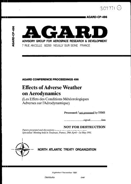
AGARD CONFERENCE PROCEEDINGS 496
Effects of Adverse Weather
on Aerodynamics
(Les Effets des Conditions M6t6orologiques
Adverses sur l’A6rodynamique)
Processed 1 not Drocessed by DIMS
.. .. .... .. .... .. .. .... .. .... .... signed. .. .. .... .. .... .. .date
NOT FOR DESTRUCTION
..._ - .-”- y,IIIII.. - _.”-.
Papers presented and discussions t .-.- _.
Specialists’ Meeting held in Toulouse, France, 29th April-1st May 1991.
I
NORTH ATLANTIC TREATY ORGANIZATION
Publiaharl nacnmhnr 1991
Distributioi over

ADVISORY GROUP FOR AEROSPACE RESEARCH 81 DEVELOPMENT
7 RUE ANCELLE 92200 NEUILLY SUR SEINE FRANCE
AGARD CONFERENCE PROCEEDINGS 496
Effects of Adverse Weather
on Aerodynamics
(Les Effets des Conditions Metkorologiques
Adverses sur YALrodynamique)
Papers presented and discussions held at the Fluid Dynamics Panel
-6
Specialists' Meeting held in Toulouse, France, 29th April-1st May 1991.
- North Atlantic Treaty Organization
Organisation du Traite de I'Atlantique Nord
I

The Mission of AGAlRD
According to its Charter, the mission of AGARD is to bring together the leading personalities of the NATO nations in thi: fields
of science and technology relating to aerospace for the following purposes:
-Recommending effective ways for the member nations to use their research and development capabilities for the
common benefit of the NATO community;
- Providing scientific and technical advice and assistance to the Military Committee in the field of aerospace research and
development (with particular regard to its military application);
Continuously stimulating advances in the aerospace sciences relevant to strengthening the common defence posture;
- Improving the co-operation among member nations in aerospace research and development;
-Exchange of scientific and technical information;
- Providing assistance to member nations for the purpose of increasing their scientific and technical potential;
- Rendering scientific and technical assistance, as requested, to other NATO bodies and to member nations in connection
with research and development problems in the aerospace field.
The highest authority within AGARD is the National Delegates Board consisting of officially appointed senior representatives
from each member nation. The mission of AGARD is carried out through the Panels which are composed of experts appointed
by the National Delegates, the Consultant and Exchange Programme and the Aerospace Applications Studies Programme. The
results of AGARD work are reported to the member nations and the NATO Authorities through the AGARD wits of
publications of which this is one.
Participation in AGARD activities is by invitation only and is normally limited to citizens of the NATO n .I t' ions.
The content of this publication has been reproduced
directly from material supplied by AGARD or the authors.
Published December 1991
Copyright 0 AGARD 1991
All Rights Reserved
ISBN 92-835-0644-8
Printed by Speciulised Printing Services Limited
40 ChigweN Lune, Loughton, Essex IGIO 3TZ

AGARDOGRAPHS (AG)
Design and Testing of High-Performance Parachutes
AGARD AG-319, November 199 1
Recent Publications of
the Fluid Dynamics Panel
Experimental Techniques in the Field of Low Density Aerodynamics
AGARDAG-318 (E),April 1991
Techniques Experimentales Likes a I’Aerodynamique a Basse Densit6
AGARDAG-318 (FR),April 1990
A Survey of Measurements and Measuring Techniques in Rapidly Distorted Compressible Turhulent Boundary Layers
AGARDAG-315,May 196‘9
Reynolds Number Elfects in Transonic Flows
AGARD AG-303, Decembcr 1988
REPORTS (R)
Aircraft Dynamics at High Angles of Attack Experiments and Modelling
AGARD K-776, Special Course Notes, March 1911 1
Inverse Methods in Airfoil Design for Aeronautical and Turbomachinery Applications
AGARD R-780, Special Course Noies, Novcmber 1990
Aerodynamics of Rotorcraft
AGARD R-781, Special Course Notes, November 1990
Three-Dimensional Supersonic/Hypcrsonic Flows Including Separation
AGAKD R-764, Special Course Notes, January 1990
Advances in Cryogenic Wind Tunnel Technology
AGARD R-774, Special Course Noies, November 1989
ADVISORY REPORTS (AR)
Air Intakes for High Speed Vehicles
AGARD AR-270, September 1991
Appraisal of the Suitability of Turbulence Models in Flow Calculations
AGARD AR-291, Technical Status Review, July 1 99 1
Rotary-Balance Testing for Aircraft Dynamics
AGARDAR-265,Reportof WG 11,December 1990
Calculation of3D Separated Turbulent Flows in Boundary Layer Limit
AGARDAR-ZSS,ReportofWGlO, May 1990
Adaptive Wind Tunnel Walls: Technology and Applications
AGARDAR-269,Rcportof WG12,April 1990
CONFERENCE PROCEEDINGS (CP)
Elfects of Adverse Weather on Aerodynamics
AGARD CP-496, December 199 1
Manoeuvring Aerodynamics
AGARDCP-497,Novcmber 1991
Vortex Flow Aerodynamics
AGAKD CP-494, July 199 1
Missile Aerodynamics
AGARD CP-493, October I990

1-4
the stall protection and the "Alpha- Floor"
system.
Fig 22
The stall protection system enable the pllot
to pitch up the aircraft up to maximum lift,
without any risk of excursions to higher
angles of attack:steady flight at this maxi-
mum angle of attack is possible,without
needing skillness.
The "Alpha-F1oor"system takes Care Of pre-
venting high rate of sink usually met at
high angles of attack :the maximum available
thrust is automatically triggered when A.0.A
exceeds a figure depending on the configura-
tion,and when the stick is fully deflected
aft.
These protections appear as one of the
major weapons of the pilots against stcong
windshears,since they enable them to apply
the right procedure without worrying about
the stall or high rate of descent which may
endanger the aircraft.
2.4.Experimental programmes or studies
Fig 23
Paper (16) from BOERET and WINTER, Germany,
presents the experimental DORNIER 28 TNT
implementing the "OLGA" system to improve
passenger comfort while flying through
gcsts.1t presents a very interesting ana-
lysis of frequency response of aircraft
structure, and human body.
SESSION 3 - VISIBILITY
3.2.Subjects adressed:
The objectives of this Session were only
partially covered ,with two papers adressing
visibility measurements , and one worthwile
mentioning , Paper (20) from WRIGHT, USA.
This paper points out the real need ,when
flying helicopters at low altitudes,in
darkness or bad visibility ,of a proper
interface between man and outside world,
which is still not provided.It points out
that, In addition to the usual sensors
providing adequate vision of the hori-
zon in the direction of the flight
(flight vector),there is a need of a good
coverage of the field of view below the he-
licopter,not yet provided.
3.2.Gaps of this session :
The following very common factors produ-
cing poor visibility were not covered:
- clouds and precipitations,rain
drizzle,fog (in weather flying)
- smoke, smog (solid particles such as
those above a battlefield,or above indus-
trial factories,sometime mixed up with
clouds 1
sand storms (often met in deserts)
Nevertheless these problems have already
been studied in AGARD , in particular it
Ck" _i_"
+h>+
-"- "C
^F *h- CC..A.. r r-.. ~
The title of this study was"Al1 weather
capability of combat aircraft".The follo-
wing comments may be extracted from the
unclassified part of the conclusions of
this study:
(3)- confirmation is given of the very
specific use of all infrared sensor systems
for dry air nights.The range reduction in
weather 1s such that it cannot be seri,>usly
envisaged to use them for precise tasks in
weather,such as take-off and landing.
(b)- electromagnetic systems are liar
more promissing:the key factor is the wave
1enath.comoared to the dimensions of w,Hter
~ I .
particles,droplets or ice crystal.It is
feasible to select the right wavelength for
optimum transmission :best transmissions
are given by VHF frequencies :millimetr-ic
wave radars provide quasi optical picture
definition while having a range far be.i.ter
than present infra-red systems,but stil~l
not sufficient in spite of the progress made
in the emitting power.
For navigation only,when the image of a
target or obstacle is not required,widely
used Air Traffic Control Radar systems,operating
on longer wavelength,have proven
their efficiency ,from a long time ago.
New positioning systems of very hi.gh
accuracy,such as the NAVSTAR Global Positioning
System.operating from a set of
Earth Satellites,or local radio electrical
systems having the same frequency,but operating
from a set of ground stations,such as
the TRIDENT (Thomson,France) are very
promissing to provide new navigation ai.ds
used in all flight phases,including take-off
and landing which require the highest accuracy.
For all these electromagnetic Systems
stealthiness remains a problem.
SESSION 4.ICING
Icing research and technology
In this session paper (22) from REINMANN
SHAW and RANAUDO,USA,on NASA's programme
on Icing Research and Technology meets the
._
challenae of arovidina in 22 waaes a vc!rv
extensive presentation of almost all subjects
related to icing.
Fig 25
(a) Physical mechanism of icing:
this mechanism involve a number of parame-
ters: airspeed,outside air temperature,alti-
tude,cloud liquid water content and concen-
tration,cloud droplet size distribution,
size or scale of models ar aircraft expo-
sed to icing,Mach and Reynolds Numbers,etc..
Ice formed in flight over the the air-
craft skin results from supercooled water
droplets impacting the airframe surface at
the flight speed.
A number of types of ice may resu1.t
from variations of the above parameters,
mainly liquid water concentration and
droplet size distribution in clouds.
Adhesion on the skin depends on the type of
icing,and roghness of surface.Basic mecha-
nical properties of ice accreted is (11
tensile (Young's module) (2)Shear (adhesion)
(3) peeling properties.

I
I
i
I
(bl Protection against icing
With the decrease of available hot air
bleed of new fan engines, there is a need
to develop new deicing systems using less
bleed,or more efficiently,or newer systems
relying on other sources of energy.
Fig 26
New systems are being developped based on
electrical capacitor discharge,using exter-
nal boots on the surface to protect,such as
EleCtrO-Expulsive Separation System, 01
Eddy Current Repulsion Deicing Boot,or
installed inside the airframe, such as the
Electromagnetic Impulse Deicer.Al1 these
systems provide very short duration impulses
but high forces, and have been foun to be
very efficient.
(cl Computation of icing accretion :
aircraft performance degradation:
Prediction of airfoil aerodynamic performance
degradation due to icing is now made
possible with the high capacity computers
~
I of to-day.The code of the method used at
I
j
~
I
NASA LEWIS is named "LEWICE".It uses invis-
cid flow equations,and determines the free-
zing point,by solving co-tinuity and energy
equations in each control volume of the flow.
Comparisons with experience give confi-
dence in this code at least for the low
incidences :the Authors state that viscous
fluid equations will have to be used for
better consistency with experiments at
higher angles of attack. close to CL max.
Fig 27
(a), Icing testing
The main ground testing means mentioned by
REINMANN SHAW and RANAUDO is the NASA
LEWIS Icing Research Wind Tunne1,which is
the largest refrigerated tunnel in the world
capable of testing big models of aircraft,
helicopters, wing profiles etc...
Flight test research is conducted at NASA
LEWIS using a modified TWIN OTTER imple-
menting modified deicing systems instead df
the basic ones.Wings and gear Struts are
used to flight test ice accretion and new
deicing systems
Associated measurements involve a number
of devices such as :
- forward scattering spectrometer probe
- optical array probe
- phase doppler particle analyser
(to measure the dimensions of water par-
ticles).
Fig 28
(e) New physical models:
REINMANN SHAW and RANAUDO made the propo-
sal of a new physical mbdel for ice accre-
tion, shown by this figure.
SESSION 5.ELECTROMAGNETIC INTERFERENCES
This Session included three papers ,each of
them bringing complementary information to
the others.The followin items are worthwile
mentioning: they are extracted from Paper
(26) from FISHER, USA
Fig 29
Surprisingly,sevez-e lightning strikes can
be found where one would not expect them:
- Aircraft lightning strikes occur in
both thunderstorm and non thunderstorm con-
ditions.
- The thunderstorms regions with the
highest probability for an aircraft to expe-
rience a direct lightning strike were those
areas where the ambiant temperature was
- 40DCelsius, where the relative turbulence
and precipitation intensities were characte-
rized as negligible to light.
- The non -thunderstorm regions with
the highest probability for an aircraft to
experience a direct lightning strike were
those areas where the ambient temperature
+
was between -10°C in rain, where the rela-
tive turbulence intensity is characterized
as negligible to light.
- Most aircraft lightning strikes are
triggered by the vehicle itself.Lightning
strikesin which the aircraft intercepts
a naturally-occurring lightning flash also
occur.predominantly at lower altitudes.
- The presence and location of light-
ning do not necessarily indicate the pre-
sence or location of hazardous precipita-
tions and turbulence.
During the discussion of this session the
Special Regulatory Conditions applied to
the A320 , giving the Electromagnetic
Interference Model , and the Lightning
model to take into account for Airworthi-
ness Certification,were presented by
the Technical Evaluation Reporter as
very severe threats.The A320 was demon-
strated as not effected by.these threats,
originated either by "natura1"events ,
such as lightning, or from equipments
made by man ( powerfull ground radio
stations, radars ,etc...l

1-8
3
TABLE I - DIGITAL FLIGHT WCORDS FROM AIRLINE ENCOUNTERS WITH SEVERE ATMOSPHERIC
DISTURBANCES
RATE
611 5
11/75
418 1
7/82
10183
11/83
1/85
2/85
U85
8/85
8/85
11/85
3/86
4/86
7/86
9/87
11/87
1/88
3/88
,!aaAEC
LlOll
DClO
DClO
DClO
DClO
LlOll
B747
B747
B747SP
LlOIl
MD80
B747
B747
DClO
A300
LlOl!
A310
0767
B767
JFK, NY
Calgary, Canada
Hannibal, MO
Morton. WY
Near Bermuda
Offshore SC
Over Greenland
Over Greenland
Offshore CA
DallasiFt.Worlh, TX
Dallas/Ft.WorIh, TX
Over Greenland
Offshore Hawaii
Jamestown, NY
West Palm Beach, FL
Near Bermuda
Near Bermuda
Chicago, IL
Cimarron, NM
OPERATlON
Go-around
33,000'
37,000'
39,000'
37,000'
37,000'
33.000'
33,000'
41.000'
Landing
Go-around
33,000'
33,000'
40,000'
20,000'
31,000'
33.000'
25.000'
33.000'
FROM PAPER 3 WINGROVE BACH SCHULTZ . USA
4
(a) HIGH-ALTITUDE TURBULENCE
W
(b) LOW-LEVEL MICROBURST
Figure 1. Two types of severe atmospheric disturbances.
lx."ME
Microburst,
Clear air turbulence
Clear air turbulence
Clear air turbulence
Convective turbulence
Clear air turbulence
Clear air turbulence
Clear air turbulence
Wind shear
Minoburst
Microburst
Clear air turbulence
Clear air turbulence
Wind shear
Convective turbulence
Convective turbulence
Convective turbulence
Convective turbulence
Clear air turbulence
FROM PAPER 3 WINGROVE BACR SCHULTZ . USA

5
(81 HANNIBAL. MO. APRIL
lbl MORTON, WY. JULY
37,000 11. 39.000 11.
lcl SOUTH CAROLINA, NOVEMBER [dl CALGARY, NOVEM8ER
37.000 11. 33.000 11.
Figure 4. Overview'of seven: turbulence encounters a1 cmisc
altitudes.
FROM PAPER 3 WINGROVE BACK SCHULTZ.. USA
NOVEMBER
-70 -50 -30
TEMPERATURE,%
: (dl CALGARY,
NOVEMBER
-70 -50 -30
TEMPERATURE.%
FROM PAPER 3 HINGROVE BACH SCHULTZ . USA

1-20
27
CALCULATED CWAR I SON EXPERIENTAL
Lwc = 1.02 gn/M3 "D = 12 wti V, = 52 WSEC T, -26 OC
CALCULATED CWARISON EXPERIENTAL
LWC = 1. M gun3 WD = 20 PM v, = 89 USEC T, = -11 OC
FIGURE 10. - CWARISON OF ICE SHAPE PREDICTIONS WITH AIRFOIL ICING DATA.
FREEZING AT
FROM PAPER 22 REINMANN SHAH RANAUDO - USA
- I
ICE HILL GROWING UNDER
-
-WATER FILM:.,-- .-
*TOP
'OF ICE HILLS. '
,, ICE HILLS GROW BY FREEZING
CLOUD MOPLETS
.I ._
-_
-: ..
- HEAT TRANSFER COEFFICIENT
(B) FREEZING OCCURRING.
FIGURE 15. - PROPOSED NEW PHYSICAL MOML FOR ICING PROCESS.
-

Pressure 24
altltude, 16
Pressure 24
altitude, ,6
29
1496 penelratlons 4239.5 mln 707 strikes
Mean = 7.0 km
Meon = 8.7 km
3 (22 900 11)
(29 600 11)
40 Ll0
0 80 240 400
Penetration
714 strlkes
1496 penetratlor
I
u
0 2 4 6 9 1 0
Slrikeslpenetratlon
,
,200 to 4OOHegaHertz 50
40OHegaHertz-lGlgaHertz 400 6
1 to 3 GlgaHertz 200 6
3 to 0 GlgaHertz 400 6
18 to 30 GigaHertz
0 200 600 1000 0 40 120 200
Duration, mln Strikes
714 strlkes 185 nearby llashes
4239.5 mln Mean = 8.6 km
c
LL
0 .30 .90 1.50 0 8 16 24 32 40
Slri keslm in Nearbvs
Fig 4 - THUNDERSTORH PENETRATIONS AND LIGHTNING STATISTICS
AS A FUNCTION OF PRESSURE ALTITUDE FOR NASA STORM
HAZARDS 1900- 1986 FROM PAPER 26 FISHER . USA
EFFECT OF EXTERNAL RADIATIONS ON AIRCRAFT
SYSTEMS
(extracted from the J.A.A. Requirements applied to
the A320 )
The external threat frequency bands and corresponding
average end peak levels that shall be used to establish
the internal threat levels are defined as follows
Frequency range
600 6
(28 100 tt)
P
30
1-21

3-4
effect on ice types similar to an increase
in airspeed or reduction in liquid water
content, producing more brittle opaque ice
which shed more easily. Different
temperatures produce ice of a different
nature. Rime ice forms at low temperatures,
is smooth, opaque and tends to follow the
shape of the surface on which it is
building. Glaze ice forms at temperatures
approaching OOC, is clearer and comprises
forward facing "feathers" which give the
classic horned shape. Glaze ice is
generally a greater problem since it has a
larger effect on drag and damage potential
if the ice is released. But it tends to be
more brittle and is more readily shed. The
appearance, net quantity, shape,
distribution, relative location, physical
properties of the ice are a function of
ambiant conditions, the collecting surface
and surroundings, the external forces.
Macroscopic and microscopic observation of
ice accretion concluded that:
- the physical and mechanical properties
of ice formed by accretion are a
function of formation conditions.
- the effects of altitude, rotational
speed, vibration, heat input, material
type and surface finish may also
influence ice properties, and these
phenomena should be investigated.
- alternative techniques for microscopic
observation should be investigated.
The author also explained the research on
static vane sets. The vanes were set at
different incidences and the test run for
30 minutes at the highest air velocity of
119 m/s. The comparison was made on the
result of pressure drop, platted non-
dimensionally in the form:
where bP = measured pressure drop
bPo- initial bP
An example of the pressure drop's
evolution, indicating the blockage is shown
in figure 17. For different speeds and
temperatures, the closely spaced vanes are
more prone to blockage and ice bridging,
and the blockage is highly dependent on
shedding propensity. We also mention from
this report the research on the adhesive
strength of ice formed by accretion. These
experimental investigations determined the
bond strength of ice build up on rotating
collectors. The ice mass resulted in a
centrifugal shedding force recorded by
strain gauges on the collector arm front
and back faces (figure 18). It was noted
that failure tended to be cohesive,i.e.
failure occurred within the ice at lower
temperatures. At higher temperatures
adhesive failure 0ccurred.i.e. the bond
between ice and metal surface was broken.
The transition occurred between -6OC and
-10-C air temperature, which corresponds to
the transition between rime and glaze ice.
Tests were carried out to investigate the
effects of LWC (0.5 to 2.5 g/m3), droplet
size (15 to 30 pml, impingement angle,
surface preparation (clean or greased) and
coatings.
Mr. E. Carl presented the icing test
facility operated at Barcley in the U.K. by
Aero and Industrial Technology Limited
(AIT)(32). This plant is operated on a
normal commercial basis and is CAA
approved. Figure 19 shows the main plant
schematically, and the main capabilities
are: airflow of up to 5.7 kg/s at a
pressure down to 38 kPa, corresponding to a
Pressure altitude of 7620 m. At higher
altitudes up to 15240 m the airflow is
reduced at 3.4 kg/s. Air temperature is
supplied in the range -65-C to +75"C and
rapid changes in air pressure and
temperature can be achieved. The engine
test cell is 12.2 m long by 4 m diameter
giving a normal working space 7.9 m long by
1.8 m diameter. Based on the JAR and 'the
FAR the correct icing conditions, such as
air velocity, pressure, temperature, water
content and droplet size are set for
predetermined times. In addition there may
be a requirement for testing the effect of
ice blocks ingested by the engine. This is
done by either allowing the ice accretions
to shed as in service or by producing ice
blocks in a refrigerator and injecting
pieces of a known size into the item. A
special gun can also produce and inject
hailstones. The configuration of the test
sections is shown in figure 20. Recently a
laser equipment (Malvern 2600C) has been
installed for water droplet measurement.
Scott Bartlett presented the AEDC
facilities (31). These are altitude engine
test facilities covering a wide range of
mach numbers, pressure altitudes, inlet
temperatures and icing conditions. The
free-jet and direct-connect testing modes
are possible. In direct-connect tests one
can test engines requiring an airflow of
340 kgls at sea-level. Bigger engines can
be tested at increasingly higher altit.udes.
As many icing problems occur at reduced
power setting meaningful icing teste can be
conducted an engines for which the maximum
airflow is above the facility capabili.ty.
Figure 21 indicates the test limits in
pressure and temperature. An interesting
detail is the LWC required in a direct
connecting test. Figure 22 shows that the
streamtube in the real flow in front of the
inlet is convergent or divergent depending
on the flight mach number and the mach
number in front of the fan. Thus air
density increases or decreases and the LWC
in g/m3 is modified. The LWC in the airflow
of the straight connecting tube must be
adapted to simulate the required content in
the real upstream conditions set by the
regulations. The icing cloud's uniformity
is evaluated by the ice accreted on a
calibration grid. This technique has been
automated a2 AEDC by application of
ultrasonic piezo-electric transducers.
These are integrated into the grid and the
ice thickness and growth rate on the
transducer is calculated in real time by a
signal processing system. This automation
greatly reduces time for icing test
preparation. The measurement effort of the
cloud's liquid water content uniformity
aimes at developping electro-optical
diagnostics to replace the pieza-electrical
transducers on the calibration grids. Using
fluorescent dve in the water and excitino
illustrated in figure 23 obtained at AEDC.
The test facility at Pyestock was
presented by Hr Holmes of the RAE (34). The
capability for icing tests was incorporated
at the design stage of two of the altitude

test cells intended for aero-engines. There
is still work to do an improving the icing
tests and one of the most important
elements is the simulation of a defined
cloud. Some icing clouds consist of a
mixture of supercooled water droplets and
particles of dry ice. These can be produced
at Pyestock based an different techniques
for the production of both components: ice
particles are produced by milling chips of
prepared ice blocks and introduced into the
main flow upstream of the liquid water
injection. There is a problem in measuring
the uniformity of the droplet size
distribution in a 2.6 m diameter cell.
Therefore at RAE they calibrate individual
nozzles in a controlled environment in a
low speed wind tunnel especially adapted
for this purpose. The two cells have large
test chambers of 6 m and 7.6 m diameters,
the latter can accomodate a helicopter
without rotors. A majority of the aeroengine
testing is done in connect mode, but
it is more realistic to do it in free jet
mode. The icing cloud is produced by a
number of airblast water spray nozzles on
rakes . A new rake for testing of large
engines requires 310 nozzles for a 2.64 m
duct. Five channels of closed circuit TV
are available for remote viewing: one
channel is a strobed view of rotating parts
whilst highspeed cine up to 1200 frames per
second records the ice shedding and
particle trajectories. Measuring the water
content and droplets’ diameter in the real
test cells close to the engine is the
preferred solution but it is very difficult
to achieve in large scale engineering
environment with delicate instruments. The
alternative solution at Pyestock is an open
circuit wind tunnel with a 0.31 m2 working
section and 80 m/s wind speed. Spray
nozzles characteristics (figure 24) show
the nozzles’ operational limits. Another
problem is the cooling down of the droplets
in the airflow. The water is injected at
20‘C to prevent freezing on the nozzle; are
the droplets supercooled at the time they
impact on the target? The state of the
droplets determines the ice accretion
forms. A 10 micron droplet comes to thermal
equilibrium in a -5-C airflow in under a
meter, but a 30 micron droplet might
require 5 meters. Thus the distance between
the spray rake and the target needs to
exceed 5 meters.
Hr Creismeas of C.E.Pr reported on a
numerical code developed at C.E.Pr. and
ONERA (30). As said in above paper the
distance between spray rake and test item
is in excess of 5 m and there can be a
significant modification in the droplets’
mean diameter. The test requires a given
mean droplet diameter and it is useful to
have a method to predict the evolution. The
theory is based on the thermal exchanges
between the liquid water and the gasflow,
taking into account the hygrometry. This
numerical code is named H.A.GI.C
(Modelisation et Analyse du GIvrage en
Caisson). The equations are based on the
continuity, momentum and heat equation. The
drag force of the droplet in airflow is
based on the value of Cx which is taken as:
(24/Re). (1+0.15
3-5
Theoretical results were compared with
experimental results. The starting section
is 0.25 m where mass distribution in
diameter intervals are given in table 2 for
4 Cases. The diameters in a section 1.95 m
from the injector were measured and
calculated and figure 25 gives an example
of the comparison.
5. Ice relevant cloud physical varameters.
Since 1983 the icing of aircraft is
investigated in the DLR - Institute for
Atmospheric Physics using an icing research
aircraft (33). The aim is to get
information about the dependance of the
icing relevant cloudphysical parameters on
cloud type and the height above cloud base.
The total water content (fluid and solid
particles), the median volume diameter and
the temperature T were collected during
vertical and horizontal flight through
clouds. A result is shown in figure 26. The
TWC of clouds of a high pressure area
increases about linearly with height above
cloud base. Its maximum is located just
below the cloud top and has values between
0.40 and 0.50 g/m3. Temperature is
decreasing with height and the median
volume diameters (MVD) are rather small and
are situated between 11 and 23 pm. The
phase of the particles is always fluid. The
MVD of clouds in the range of a Warm front
fluctuates strongly between small and large
values and maximum values are between 100
and 460 pm. The phase of the particles in
clouds in the range of a warm front would
vary between fluid and solid.
6. Low temperature and fuel vroblems.
The low temperature operations could
impact aircraft missions as the fuel can
form solid wax precipitates which may cause
plugging of filters or blockage of fuel
transfer lines. The Naval Air propulsion
center of Trenton was concerned with the
problem of availability of the F-44 (JP5)
fuel. This fuel with very low freezing
point accounts for only a small fraction,
less than 1% of total refinery production.
The relaxation of the freezing point
specification to that of the commercial
Jet-A specification would lead to a higher
fraction of the crude (25).
This study requires the determination
of the fuel temperature in the fuel tanks
which is very expensive if it has to be
done experimentally. NAPC looked for a CFD-
code that could be modified to handle the
calculations. They chose the PHOENICS 84 as
the base code performing fluid-flow, heat
transfer and chemical reaction calculations
simultaneously. The major developments are:
optimum grid selection, turbulence
modelling, phase change modelling and
expert system. The user-friendly menu
driven format allows the user to operate in
a menu driven step-wise format, depicted in
figure 27, where he has to input the
dimensions of the tank and the amount of
fuel desired. The boundary conditions are
either the experimental skin temperature of
the tank, or the calculated skin
temperature based on air temperature and
air speed. Figure 28 compares test and
calculated data. The model predicts
accurately, in both two and three

3-6
dimensions, fuel temperature profiles. The
accuracy of the fuel holdup is not as good
as that of the fuel temperature because
holdup was shown to be a somewhat random
phenomenon. The model is currently used to
predict the effect of higher freeze point
fuels on naval aircraft mission
performance.
A second danger of the cold fuel is
due to the presence of water dissolved in
the fuel. This water under the form of ice
crystals can block the filters, the fuel
control and change the flow passages in the
heat exchanger air-fuel. Mr Garnier of
SNECMA (23) explained the mathematical
model based on a heat balance oil-fuel to
predict the fuel temperature during the
take-off phase and cruise flight. This
model was verified on a test bench built at
SNECMA to verify the model and on an
aircraft equipped with four CFM-56, that
was put in the climatic chamber of EGLIN
(Florida) where the temperature was lowered
to between -21OC and -54-C.
1.
2.
3.
4.
5.
6.
7.
a.
9.
10.
11.
12.
13.
14.
15.
16.
17.
18.
Low Temperature Environment Operation
of Turbo Engines - Hilitary Operator‘s
Experience & requirements by Summerton
Fighter Operations in the Far North by
A.L.Smith.
Analyse des Problemes de Demarrage par
Temps Froid avec les Turbomoteurs
d’Melicopt&re de type ASTAZOU
par W.Pieters.
Avions d’Affaires Hystere-FALCON -
Experience Operatiannelle par Temps
Froid par C.Domenc.
Vulnerability of a Small Powerplant to
Wet Snow Conditions by R.Meijn.
Ice Tolerant Engine Inlet Screens for
CH133/113A Search h Rescue Helicopters
by R.Jones and P.K.Scott.
Cold Starting Small Gas Turhines - An
Overview by C.Rodgers.
Cold Start Optimization on a Hilitary
Jet Engine hy H.Gruber.
Cold Weather Ignition Characteristics
of Advanced Gas Turbine Combustion
Systems by S.Sampath and 1.Critchley.
Cold Weather Jet Engine Starting Stra-
tegies Hade Possible by Engine Digital
Control Systems by R.C.Wibbelsman.
Cold Start Investigation of an APU with
Annular Combustor and Fuel Vaporizers
by K.H.Collin.
Control System Design Considerations
for Starting Turbo-Engines during Cold
Weather Operation by R.Pollak.
Cold Start Development of Hodern Small
Gas Turbine Enaines at PWC
by D.Sreitman and F.Yeung
Design Considerations based upon Low
Temperature Starting Tests an Hilitary
Aircraft Turbo-Engines by M.-F.Feig.
Climatic Considerations in the Life
Cycle Hanagement of the CF-18 Engine
by R.YI.Cue and D.E.Muir.
Application of a Water Droplet Trajec-
tory Prediction Code to the Design of
Inlet Particle Separator Anti-Icing
Systems by D.L.llann and S.C.Tan.
Captation de Glace sur Une AUbQ de
Prerotation d’Entr6e d’Air
par R. Henry et D. Guffond.
Development of an Anti-Icing System for
CONTENTS OF THE 76th SYHPOSIUM
Fuel at cold temperature can also
impact the engines’ starting capabilities.
This is due to the low vapour pressure and
the low viscosity. The droplet mean
diameter increases and the fuel evaporation
rate is inversely proportionate to the
square of the droplet size (7,9,22). Figure
29 shows that the minimum fuel air ratio
for ignition has to be increased with
higher viscosity, thus lower fuel
temperature. Three papers: GE (lo), APU for
the Tornado (11) and PW (12) explain the
improvements in the starting capabilities
with new fuel control schedules related to
the ambient conditions.
The flame propagation model in
heterogeneous phase must take into account
the droplet diameters and droplet
distribution, the temperatures and
pressures, the fuel air ratio, the
evaporation and the turbulence. In paper
(24) this flame propagation is studied in
the case of a multicomponent fuel to
compare it with the case of a single
component idealization.
the T800-LHT-800 Turboshaft Engine
by G.V.Bianchini.
19. Engine Icing Criticality Assessment by
E.Brook.
20. fce Ingestion Experience on a Small
Turboprop Engine by L.W.Blair,
R.L.Miller and D.J.Tapparo.
21. Fuels and Oils as Factors in the
Operation of Aero Gas Turbine Engines
at Low Temperatures by G.L.Batchelor.
22. The Effect of Fuel Properties and
Atomization on Low Temperature Ignition
in Gas Turbine Combustors by
D.W.Naegeli, L.G.Dodge and C.A.Moses.
23. Givrage des Circuits de Carburant des
Turhoreacteurs par F. Garnier.
24. The Influence of Fuel Characteristics
on Heterogeneous Flame Propagation by
M.F.Bardan, J.E.D.Gauthier and V.K.Rao.
25. The Development of a Computational
Hodel to Predict Low Temperature Fuel
Flow Phenomena hy R.A.Kamin, C.J.Nowack
and B.A.Olmstead.
28. Environmental Icing Testing at the
Naval Air Propulsion Center
by W.H.Reardon and V.J.Truglio.
29. Icing Research Related to Engine Icing
Characteristics by S.J.Riley.
30. Hodelisation Numerique de l‘lvolution
d’un Nuage de Gouttelettes d’Eau en
surfusion dans un Caisson Givrant par
P.Creismeas et J.Courquet.
31. Icing Test Capabilities for Aircraft
Propulsion Systems at the Arnold
Engineering Development Center by
C.S.Bartlett, J.R.Moore, N.S.Weinberg
and T.D.Garcetson.
32. Icing Test programmes and Techniques by
E.Carr and D.Woodhouse.
33. Documentation of Vertical h Horizontal
Aircraft Soundings of Icing Relevant
Cloudphysical Parameters by H.E.Hoffman
34. Developments in Icing Test Techniques
for Aerospace Applications in the RAS
Pyestock Altitude Test Facility by
M.Holmes, V. E. W. Garrat and R.G. T. Drage.
35. Entree d’air d’HelicoptSres: Protection
pour le vol en Conditions Neigeuses ou
Givrantes par X.de la Servette et
P. Cabrit.

Fig 1: Positions and fields of view of cameras
mounted in the air intake duct
BLEEDIBYPASS DOOR
,
NO. 2 RAMP NO. 3 RAMP
RAMPS LOWERED IHIGH MACH CONDITION1
NO. 2 RAMP
BLEEDIBYPASS DOOR
NO. 3 RAMP
RAMPS STOWED [LOW MACH CONDITION1
Fig 2: Engine inlet duct F 14
Fig 3: Installation ice accretion on CT7 Turboprop
/ Dischargelo /
IPSwenge , // war
/
/ f /
Fig 4: Inlet Particle Separator system (IPS)
Airflow
20% of Chord point
IPS scavengevane cross-senion
TE90-2187
Fig 5: Required ice free surfaces
Fig 6: Preliminary Flight Rating anti-ice
thermal survey instrumentation

8-E

tar = -5°C
\
tar = 0°C
3
Fig 12: LWC=O,bg/m ; DMV=20 m Mean Diameter
Y :
FREE JET
DIRECT CONNECT
Fig 13: Icing Test inlet configurations
RUMIOIFICATIGN
11
- 130
y:
u
Y
D *IO
e
z
I- -10
I- Y
=
d
- -30
4
I-
o
I- -50
- E
I- =
I _-
e
Y=
5.0
4.0
3.0
-
= 1.0
D
4
0.0
(12-45)
fW POINT SENSOR OlSlRlBUllON
(SCREEN
ABLE SINGLE
SPRAT EARS
OTAllNE CILINOER
CALIBRATION
[ ~ ~ ~ % \ O V l E CAMERA
Q
Fig 14 :TYPICAL CALIBRATION/TEST ARRANGEMENTS
Mean Effective Drop
(,s.q5)/~iamefer Raws (microns)
I
Fig 15: NAPC Icing capabilities
TABLE 1: SEA-LEVEL ANTI-ICING CONDITIONS (MIL E 005007E (AS))
3-9

3-12
.S~)eciIy Tank Dimensions
_1
Specify Tank Wall Characteristics
' .c
I inwf Time VaryiG 0oundsry Condition8
tank skin tem~eraturee if available
Specify external heat lranaler coellicient and recovery
1emL7erature DiOtilF
-50 '
Y .\ \
m-
,002
KINEMATIC VISCOSITY. cSt
Fig 29a: Correlation of mimimum fuel-air ratio for
ignition with viscos:ity for two atomizers
M 65
.
E
0 2P.l
n JPl5
0 717: NOT. 25- Cas
* 3oz mi. 70% Car
+o
/$"
Q
4. Goroi8"E
J
AlR TEMPERATURE (K)
Fig 29b: Effect: oi inlet air temperature and fuel
type on SMD required for ignition
~42 ,-loitid temp 43.67 Lwmd:
0 Cakulatod (tank contar)
1
-- Measured bulk tompralure
100
-62
-64
-66
1
0 cakxulatod hold-up
Mewrod fop and bollom Cakulated
(baundary) tem~~ratures hold-up
-68
.70
0 40 80 120 1 80 200 240
0
280
Time, min
Fig 28: Comparison of cnlcula~ed and measured temperatures and hold-up
90
BO
70
60 %
%
50 I
8
40
30
20
10

1. -E
EVOLUTION REGLEMENTAIRE EN MATIERE DE CERTIFICATION DES
AVIONS ClVlLS EN CONDITIONS GIVRANTES
L'experience acquise au cours
certification de type et de l'utilisation en
service des avions civils a mantre qu'une
evolution des ceglements applicables a-
conditions givrantes s'av8rait necessaire. Ce
document decrit les itvolutions reglementaires
qui sont actuellement envisagees de mani$re a
maintenir au cours d'un "01 en conditions
givrantes un niveau de securite comparable B
celui qui est garanti hors givrage.
2. - RAPPEL DES EFFETS DE L'ACCUMULATION DE CIA-
CE SUR LE5 CARACTERISTIQUES ilERODYh'AMIQU8
D'UN AVION
On sait depuis fort longtemps que la
presence de glace SUP un avion degrade de
maniere significative les carncteristiques
aerodynamiques correspondantes.
I1 existe m e abondante litterature qui
traite de ce sujet et de nombreuses etudes ont
ete conduites dans le iuonde POUP en kvaluer des
consequences. Nous rappelons brievement les
principeles conclusions.
L'accumulation de glace sur un avion
grovoque :
- tine perte de portance CL a meme incidence a
qui s'accompagne d'une diminution du CLmax et
de 1'angle a (CLmax) associe.
- Une augmentation du coefficient de trainee CD.
- line degradation de la stabilite longitudinale
et de la stabilite laterale.
- D'autres caracc.Bristiques tomme la stabilite
dynamique transversale (DUTCH ROLL1 peuvent
aussi Btre affectees.
par
Gilbert CA'ITANEO
Ingeniour Nnvigant d'Essais
CENTRE DESSAIS EN VOL 13128 ISTRES AIR
4-1
L'amplitude de I'effet etudie depend de
l'epaisseur de glace. de sa forme et daw line
certaine mesure de sa rugosite (CF figures no 1
et n' 2).
Une epaisseur n&me faible peut avair un
effet considerable sur le CLmax.
L'accumulation de glace sur la profandeur
peut pmvoquer des prabl6mes graves de contrdle
longitudinal 1it.s d l'alt6ration du moment de
charniere observable SUP les avions B commmdes
de vol purement mecaniques. Des degradations
significative5 de l'efficacite de la profondeur
ne peuvent pas +tre exclues sur les avions
Bquipes de servo cammandes.

I 1
Les avions peuvent Btre plus ou mains
sensibles au givrage.
Parmi les reisons possibles qui les
differencient on peut notec :
- Que les turboceacteurs ont un domaine de "01
etendu et des performances &levees leur
permettant d'eviter ou de traverser rapidement
les zones de givrage.
- Que les systbmes de degivrage pneumatiques a
chambres deformantes (boots) n'ont Pas Une
efficacite parfaite. De la glace s'accumule
entre deux gonflages des chambres
(intercycle). Par camparaisan les systemes
d'antigivrage par soufflage d'air chaud
evitent l'accumulation de glace.
- La mise en route differbe des SyStBmes de
degivrege par application de la procedure
gacantissant 1 ' ef ficaci ti. du sys teme ,
correspond B "ne certaine quantite de glace
accumulee.
- Des conditions donnBes de givrage peuvcnt
avoir un effet different en fonction du type
de l'avion.
I1 resort de ces considerations que les
turbopropulseurs ont plus de chance d'etre
"sensibles au givrage" a cause :
- De leur domaine de vol reduit
- De leur performances limitees.
- De leur capacite limitee de prelevement de
puissance particuliereolent au decollage.
- De l'absence de servo commandes.
Par contre on observe que les profils
modernes ne paraissent pas presentsr une
sensibilite plus marquee que celle des profils
anciens.
3, - LES REGLEMENTS DE CERTIFICATION EXISTANTS
On sait que pour certifier les avions
civils de grande taille il existe
essentiellement deux reglements de base :
- La part 25 (large aeroplenes) du ti.tre 14
(Aeronautique et Espace) du Code des Lois
Federales Americaines.
- La JAR 25 (Joint Aviation Requirements).
Ces reglements sont pratiquement identiques
et sont completes par des textes additionnels :
Annexes. Advisory Circular Joint. etc....
Ainsi lorsque la certification en
conditions givrantes est demandbe en cor.focmite
avec le rbglement JAR on utilisera :
a) ktexte de base

- L'utilisation en service montre que la
meconnaissance ou le non respect. des
procedures associees a la presence de glace
peuvent conduire a des pertes de contrdle
sBveces suivies de recuperations hasardeuses
qui dans un cas extreme ant entrain6 la perte
de l'avion et de ses occupants.
Pourtant la reglementation telle qu'elle
existe parait constituer un ensemble coherent et
complet. Pendant de nombreuses annees elle a 6t.e
considepee comme suffisante et pscfaitement
capable d'atteindre l'objectif qui lui Btait
assigne : garantir une sewrite suffisante.
En realite. cette reglementation, tres
explicite sur les conditions de givrage A
etudier et sur les demonstrations relatives aw
systemes. reste extremement vague sur les
I dBgPadationS de performance et de qualites de
vol que l'on peut accepter. A titre d'exemple on
peut citer le seul paragraphe qui aborde cet
! aspect (CF ACJ 25-1419). Where ice can accrete
on unprotected parts it should be demonstrated
that the effect of such ice will not critically
affect the charactepistics of the sbroplane as
regards safety (eg Flight, Structure and
flutter). The , subsequent operation of
retractable devices should be considered."
Ces insuffisances ont conduit les autorites
franpises de certification a proposer des
textes compl8mentaires.
5.1. CENFBALITES
Les objectifs de securite des textes
existants etant parfaitement definies le choix
s'est porte SUP le maintient de ces textes et le
developpement de moyens d'intecpretation (Advi-
sory Material Joint). L'AMJ 25-1419 ainsi
developpee $'est en partie inspicee du conten"
des AMA's 52512-x et 525/5-x Blaborees par les
autorites canadiennes DOT.
5.2. CONTENU DE L'AMJ 25-1412
5.2.1. Generalites
- Les conditions atmosph6riques sont celles
definies dans l'annexe C des reglements
FAR 25 ET JAR 25 (CF annexe 1).
- Les phases de vol significatives sui-
vantes sont prises en consideration.
Decollage. montee. croisiere. attente.
atterrissage. cas de panne. Pour le
dCcollage les systemes de degivrage sont
supposes etre mis en route 400 feet,
sauf si la procedure permet explicite-
ment leur utilisation avant d'atteindre
cette altitude.
- Les essais pewent &tre effect"& avec
des formes de givre artificielles. les
resultats ainsi obtenus doivent etre
recoupes par des essais en givrage
naturel. Les formes artificielles doivent
etre dbterminees B partir de madeles de
calcul valid& par des essais (soufflerie
par exemple) et appniuves.
5.2.2. Quantites de glace accumulee
Decollage :
suppose effectue avec une panne moteur B
VEF. un rapport critique PoussAeJPoids. La
glace est accumulee sur l'ensemble des
parties captantes de l'avion a une
incidence mayenne pendant une phase de
duree determinee.
Croisiere - Attente et Atterrissage :
a) Parties no" protegbes de l'avion.
Captation jusqu'a une Bpaisseur maximum de
3 pouces avec des asperites de hauteur 3 mm
et "ne densite de 8 a 10 grains par cm2.
b) Parties pro-.
Les delais de mise en route des systemes
anti/degivrages, involontaires ou lies a la
procedure. sont pris en compte ; de meme
que la glace accumulee pendant un inter-
cycle et que la recongelation eventuelle
(runback).
Cas de panne :
LoPsque la panne affecte l'efficacite du
system de degivrage et que l'avion doit
alors quitter les conditions givrantes la
quantiti: supposCe de glace deposbe SUP les
parties protkg6es est fixee a 1.5 cm
Cas particulier du Sand Paper :
Une forme specifique de captation
correspondant a "ne faible epaisseur et une
cugosite du type papier de verre a ete
utilisee pour qualifier le camportement de
l'avion lors des manoeuvres de rendus de
mains (push overs). On Sait en effet par
l'experience SUP differents avions tels que
ATR 42. SF 340 DO 228 que Ce type
d'accretion est critique POUP la manoeuvre
consider&.
5.2.3. Essais B executer
Performances :
Etablissement des vitesses de decrochage en
vue du calcul des nouvelles vitesses
OpCrationnelles associesr. Validation des
marges entre activation des systemes de
protection (Stall warning. stick shaker) et
decrochage. Etablissement des palaires de
traini:e.

D'une man1
ulO" tren t c
degradee e
auaiites de vol.
gherale. les quali
cune caracteristique
wage naturel que ce
is de "01
,'est plus
e observee
nvec les formes artificielles. Les objectifs
definls en 5.2.4 sont donc atteints.
7.- BIWN DES ESSAIS
La campagne de certification de 1'ATR 72 en
givrage a necessite :
- 25, vols yeprksentant 47 heures POUP les essais
avec formes artificielles.
- 11 vols representant 35 heures pour les essais
en givrage naturel.
soit au total 36 "01s representant 82 heures.
I1 convient cependant de remarquer ce qui
suit :
Vols avec formes artificielles.
Un important tcevail de mise BU point des
gknerateurs de tourbillons de voilure et
d'optimisatian du seuii de declenchement du
stick pusher ont 6th rendus necessaires pour
ameliocer le comportement de l'avion a m hautes
incidences. Ce travail ne peut Btre impute ti
l'application de 1'AMJ. il represente 21 heures
de "01.
Vols en givraKe naturel.
Un certain nombre d'heures ont du Btre
cansacrees B la recherche. quelquefois
infructueuse. de conditions givrantes valables.
Ainsi qu'am essais de certification des
SystBmes antigivragefdhgivrage equipant l'avion.
Ces heures ne peuvent egalement pas Btre
imputees a 1'AMJ. elles representent environ 25
heures.
Finalement I'application de 1'AMJ entrainerait
un surplus d'environ 25 heures de "01 avec
formes artificielles et 10 heures en givrage
naturel soit approximativement 35 heures all
total.
Cette quantite est raisonnable eu hgard au coat
total d'un programme de certification complet
(entre 1000 et 1200 heures de voi). surtout si
on cansidere l'ameliorntion importante de
securite que les essais correspondants
apportent.

8.- APPLICATION DE L'AW A D'AUTRES AVIONS
A titre experimental. 1'AMJ a et6 appliquee
sur un autre avion : le FOKKER 21 ARAT (Avian de
Recherche Atmospherique et de Teledetection). 11
s'agit d'un avion FOKKER 27 madifie Par
ad jonction :
- D'une perche de nez porte capteurs (a, B. PP).
- D'une CouPonne de capteurs autouc du Fuselage
avant.
- De points d'emports de capteurs sous voilure
Ces modifications Sont destinees a des
mesupes au profit de divers organismes :
- Institut CBographique National
- Institut National des Sciences de 1'Univers.
- Groupe de TBlBd6tection Aerienne.
Les principales conclusions qui one et6
tirdes de cette etude sont les suivantes :
- Les essais de performances confirment
l'influence notable des formes de givre sur
les vitesses de decrochages (CF figure no 9).
Y
P
I
4-7

- Les formes artificielles constituent une - Les essai-s de recoupement en givrage nature1
enveloppe realiste des accretions naturelles sont indispensables et permettent notwent
de givre. d'avoir une idee de l'influence du givre SUP
la trainee (CF fiwuce no 10 evolution de la
- Sur cet avion les qualites de vol sent vitesse Vp stabilisee en palier A is0
faiblement affectees PBP le givrage.
9,- CONCLUSION
Les essais effect"& SUP deux avians
comparables du point de vue de la motorisation
et des commandes de vol mais assez differents du
point de vue des formes exterieuces tendent a
prouvep que 1'AMJ 25-1419 est bien adaptee BUX
avions du type Commuter.
Bien que les textes correspondant ne sont
pas formellement approuves a l'heure actuelle au
niveau des instances JAA. son application B des
avions =omme le JETSTREAM 4100. le SAAB 2000. le
DORNIFA 328 de meme que l'A330 et l'A340 est
envisagee sous forme de conditions speciales.
Elle contient en et'fet suffisamment d'Bli.ments
qui peuvent i-tre transposes sans difficulte des
Commuters aux Jets. Bien entendu il est
necessaire de tenir compte des paPticularites de
ces derniers et plus specinlement des systemes
de protection en incidence.
Dans l'esprit de ses auteurs 1'AM.I 25-1419
represente une exigence susceptible d'apporter
une meilleure garantie de sBcurit6 du vol en
conditions givrantes
puissance en fonction de la quatit6 de glace
accumulee).

1, - MAXIMIM CONTINU
DEFINITION DES CONDITIONS MAXIMUM CONTINU ET MAXIMUM INTERMllTENT
(ANNEXE C DES REGLEMENTS JAR 25 ET FAR 25)
Altitude Pression : 2.- WINJM INTERMITTENT
0 i 7.0 s 22 000 feet
Temperature ext6rieure :
- 30 5 ~a i o'c
Ktendue verticale mimum du nllage :
6 500 feet
Etendue horlzontale maximum du nuage :
17.4 NM
Altitude Presslan '
4 000 i zp 5 22 000 feet
Tentpepatwe exterieure :
- 30 I ~a I o'c
Ktendue hortzontale maximum du nuage
2.6 NM
Dlametre effectif moyen des gouttelettes :
Diametre effectlf myen des gouttelettes . 15 % j4 5 50 mlcmns
15 i p i 40 mlcmns
Concentration en ea" .
0.05 i C i 0.8 g/d
1.- FORMES DECOLLAGE (~es
&tat inoperants).
2 = Oft
SAT = -4'C
C = 0.5j glm3
Concentratlo" en eau
0.15 i C.5 2.9 g/m3
CONDITIONS DE CALCUL DES FORMES ARTlFlClELLES DE GlVRE SUR ATR 72
diametre des gouttelettes = 20p
VC = 81 k t (LREI = 1~
pendant ot = 60 sec
VC i 126 kt am = 7'
pendant bt = 120 sec
2.- FOWS CROISIERE
2.1 Parties no" Dmt6K6eS
systems de protection
zp = 15000 ft SAT = -12OC
diametre des gouttelettes = 2Op
vc cmiei6re max 230 kt
c = 0.38 g/m3
2.2 Partie DmteKCeS
ot = 35 mn (e = 3in ma)
zp i 15000 ft SAT = -2O'C
diametre des gOutteletteS = 20p
VC croisiere max 230 kt
~aximum intermittent c = 1.7 gr/m3
ot = 34 sec
~aximum continu
ot = 146 sec
c = 0.2 gr/m3
3 ~ - CAS DE PA"E
L ~ S conditions smt les memes que pour Ies
parties "on protegees en cmisiere main plur un
temps d'exposition moitie ot = 17 mn.
4.- FOMIES "PUSH OVERS" sur parties prot&g&es.
Configuration atterrissage
VC i 90 kt Zp i 5000 ft
Diametre des gouttelettes ZOp
Maximum intermittent
C = 2.42 g/m3
5, - RUGOSITE DES FORMES
ot = 60 sec
SAT = - 4.C
pour les accumulations impartantes
(e = 3i") :
hauteur des grains 3 mm
dewit6 a a 10 par cm2
pour les accumulations faibles (e < 5 mn):
hauteur des grains 1 mm
densit6 a A io pap CG
4-9

Summary
ICING SIMULATION
A SURVEY OF COMPUTER MODELS AND EXPERIMENTAL FACILITIES
This paper is a survey of the current methods for
simulation of the response of an aircraft or aircraft sub-
system to an icing encounter. The topics discussed
include: 1) computer code modeling of aircraft icing and
performance degradation, 2) evaluation of experimental
facility simulation capabilities, and 3) ice protection sys-
tem evaluation tests in simulated icing conditions. Cur-
rent research, which is focussed on upgrading simulation
fidelity of both experimental and computational meth-
ods, is discussed. The need for increased understanding
of the physical processes governing ice accretion, ice
shedding, and iced airfoil aerodynamics is examined.
1. Introduction
The safe operation of an aircraft under icing condi-
tions is a topic of current interest in the aerospace com-
munity. A need for development of icing simulation
methods has been identified by aircraft manufacturers
and certification authorities alike.' Reinmann, et al?
identified several reasons for the current interest in icing;
'(1) the more efficient high by-pass ratio engines of
today and the advanced turboprop engines of tomorrow
have limited bleed air for ice protection, so the airframers
are seeking more efficient systems; (2) airfoil designers
do not want their modern, high-performance surfaces
contaminated with ice, so they are intensifying pressure
to develop ice protection systems that minimize residual
ice and thereby allow the airframer to keep airfoil surface
aiea to the minimum; (3) new military aircraft requiring
severe weather capability are currently under develop
ment (4) some existing military aircraft, being used pri-
marily for training missions, are experiencing foreign
object damage @OD) due to icing conditions they would
not normally encounter in combat (5) designers of high
performance military aircraft want to avoid burdening
the aircraft with ice protection, so they want to know
where and how much ice will build on the aircraft and
whcther the aeroperformance penalties are acceptable;
(6) designers of future high performance aircraft with
relaxed static stability need to know how their aircraft
will perform with contaminated aerodynamic surfaces;
(7) littleisknownabouttheeffectsof iceaccretiononthe
by
M.G.Pntaoczuk and J.J.Reinmann
NASA Lewis Research Center
Mail Stou 77-10
Cleveland, Ohio 44135
United States
operation and performance of advanced turboprops, and
whetherornot iceprotectionwillberequired;and(8) the
FAA has certified only one civilian helicopter for flight
into forecasted icing, which implies a strong need for
support of helicopter icing.'
Satisfying these needs can require lengthy and
expensive flight test programs if unassisted by icing sim-
ulation methods. Additionally, finding icing conditions
over the full certification icing envelope can not be done
within a reasonable time frame. Thus, various methods
for simulation of icing conditions are an important and
necessary part of the design and certification of aircraft
and ice protection systems.
Initial efforts at icing simulation took place in the
late 1920's and early 30's. These activities are described
in References 3-8. World War I1 precipitated an urgent
need for research into icing simulation and ice protection
system design. In the United States, this led the National
Advisory Committee for Aeronautics, NACA, to build
the Icing Research Tunnel (IRT) at the Lewis Research
Center in Cleveland, Ohio during the early 1940's. Initial
activities in the IRT covered a broad range of icing prob-
lems. Many of these included the development of ice for-
mations on aerodynamic surfaces and the evaluation of
aerodynamic performance degradation. A complete bib-
liography of the NACA research activities during this
period is available as a NASA TM?
Icing simulation activities have increased dramati-
cally during the period from the late 1970's to today.
Wind tunnel and flight research has been conducted by
many organizations in North America and Europe. In
addition, the advent of high speed computer systems has
allowed the development of sophisticated computer sim-
ulations of ice accretion processes and resulting perfor-
mance degradation. As a result, a new role has been
created for wind tunnel and flight research, that is devel-
opment of code validation databases.
Despite the long history of icing research, there still
remains a significant number of unresolved issues in the
process of icing simulation. These issues range from the
fundamental physics of the icing process to the mecha-
nisms underlying the ice removal process. The ability of
the aerospace community to predict the effects of aircraft
icing and the performance of potential ice protection sys-
tems will be strengthened by addressing these issues and

incorporating an increased understanding of the icing
process into simulation efforts. This paper seeks to iden-
tify the issues of current icing simulation research and to
suggest how current simulation methods might be
improved.
2. The Physics of Icing and Ice Protection
2.1 Ice accretion ohvsics
Icing occurs when an aircraft encounters a cloud
containing supercooled water droplets, which impact
aerodynamic surfaces and freeze, forming non-aerodynamic
shapes on these surfaces. Incoming water droplets
can vary in size from 2 or 3 microns to over 40 microns.
Typically, smaller droplets tend to follow the airflow over
the surface while larger droplers follow more straightline
paths to the surface. Upon impact on the aircraft surface,
the water droplets can either freeze immediately or
exist as a water/ice mixture. These two conditions are
dependent on environmental parameters such as, temperature
and clood liquid water content (LWC), and on aircraft
surface conditions such as, skin temperature and
surface roughness.
The basics of the ice accretion process, as described
above, have been known for some time. However, there
are details of the process which are still not completely
understood. Recent research in these areas has focused
on development of alternatives to the physical model currently
used in ice accretion codes.The current model was
proposed by Messinger" nearly forty years ago and
includes the following concepts: in rime icing conditions
(i.e. air temperatures well below freezing and low LWC
values), all cloud droplets freeze upon impact with the
surface. In glaze icing conditions (Le. air temperatures
close to freezing and high LWC values), only a fraction
of the water will freeze upon impacr and the remainder
will run back. The close-up photography of Olsen and
Walker," as shown in Figure 1, indicates that some fraction
of the water which remains in the liquid state after
impact may not runback along the surface, as is currently
assumed. This water may remain in pools formed by the
surrounding ice, thus requiring an alteration of the current
model of the ice growth process. Splashing of
incoming water dr~plets'~"~ may occur under certain
conditions, which could result in less water on the surface
than indicated by droplet trajectory calculations. It
is also suspected that the initial conditions of the icing
process may have a significant impact on the subsequent
ice growth. Factors such as the initial surface roughness,
the surface tension at the air-water-airfoil interface, the
water droplet size, and the boundary layer transition
location can all influence the final ice
Following up on Olsen's work, Hansman, et al. l4
further studied the icing process. Figure 2 shows the test
setup used to observe ice growth on a cylinder. By illu-
minating the ice surface with a laser sheet, they con-
structed a time history of the ice profile (shown in the
middle diagram). This sequence of profiles suggested a
three zone heat transfer model that differed significantly
from the Messinger model. Hansman's model attempts to
account for the changing conditions on the airfoil surface
by tying the transition from the smooth to rough region
to the boundary layer transition.
It is hoped that by understanding the ice accretion
process more completely, some of the empiricism
present in current icing models may be eliminated. This
should result in more robust models providing simulation
of the icing process over a broader range of the icing
envelope.
2.2 Iced airfoil aerodvnamics
Ice accretions on the wing leading edge lead to
increases in drag, decreases in lift, changes in the
moment distribution, a decrease in the value of CL-.
and a decrease in the stall angle. These effects are due to
a change in the pressure disnibution on the wing and to
increased viscous losses.
From the point of view of effects on aerodynamics,
ice growths have two relevant length scales. Ice growth
structures on the scale of the boundary layer height can
be considered as roughness elements. Structures larger
than the boundary layer height and on the order of the airfoil
thickness influence the aerodynamics in different
ways and are typically referred to as ice shapes or ice
caps.
Ice shapes can result in changes in the pressure distribution
over the airfoil, development of separated flow
regions, early transition of the boundary layer, and premature
stall. Ice roughness can result in thickening and
early transition of the boundary layer, alterations to the
pressure distribution, and increased drag. Both types of
ice growth can lead to a decrease in maximum lift.
The results of Ingelman-Sundberg, et al.'5suggest
that ice roughness can result in a decrease in CL- and
that a glaze ice shape can result in an even larger decrease
for single-element airfoils. Their results alsoindicate that
roughness and ice caps produce approximately the same
level of change in CL- for high lift configurations.
Potapczuk and I3erkowifd6 have measured the changes
in lift, drag, and pitching moment for a two-dimensional
model of a Boeing 737-200 ADV wing section, in both
cruise and high-lift configurations, as ice accumulated on
the surface. Their results indicated continual increases in
the effects of ice accumulation on drag. The changes to
IiCt and pitching moment were not evident until the angle
of attack was varied from the condition at which the ice
was accumulated.

It is difticult to establish any clear trends applicable
to all icing encounters, however, it is safe to say that the
dcgree of aerodynamic degradation due to icing is depen-
dent on airfoil geometry and attitude, ice accretion time,
and icing cloud conditions. As a consequence of this
dependence, it is apparent that simulation of iced airfoil
aerodynamics is necessary to thoroughly evaluate the
behavior of a given aircraft encountering icing condi-
tions.
The changes in airfoil aerodynamics due to icing
apply equally to helicopter rotors. Bond et has
shown that rotor icing can lead to increases in rotor
torque on the order of 25 to 50 percent. Additional results
indicate that ice shedding events can reduce rotor torque
by 5 to 10 percent temporarily, thus producing loading
transients which can increase system vibration. Asym-
metric ice shedding can pose a considerable problem due
to out-of-balance conditions which may lead to high
vibratory loads on the rotor system."
2.3 Ice Protection Svstems
Thereare twoapproaches toaircraftprotection from
icing; anti-icing and de-icing. Anti-icing is the prevention
of ice growth on critical aircraft lifting surfaces,
while de-icing is the removal of accumulated ice before
significant degradation of aircraft performance. Antiicing
methods provide the greatest safety factor but
require the greatest amount of energy. De-icing methods
on the other hand may provide appropriate safety with
lower energy requirements.
Either approach to ice protection may be implemented
in a number of ways. There are essentially three
catcgories of ice protection techniques: chemical,
mechanical, and thermal. Chemical methods typically
consist of exuding some type of material on the wing surface
that mixes with the ice and depresses the freezing
point. Mechanical methods utilize various devices that
break the ice-wing surface bond by imparting a strain or
an impulse to the outer structure of the wing. Thermal
methods melt or evaporate the ice by heating the wing
surface through a variety of methods.
The conventional approach for protection of commercial
transport vehicles for the past thirty years has
becn anti-icing through the use of hot compressor bleed
air. Hot air flowing inside the wing raises the temperature
of the leading edge above a level which will allow ice to
form on the surface. Usually the temperature of the leading
edge is high enough to evaporate any water on the
surface. This prevents runhack water from refreezing on
the wing surface aft of the heated area.
But more recently, as jet engine manufacturers have
begun increasing engine by-pass-ratios to achieve higher
efficiencies, the engine cores have become smaller and
the amount of hot bleed air available for anti-icing has
5-3
shrunk significantly. First priority for bleed air is given to
cabin pressurization and air conditioning. To cope with
this loss of bleed air, airframers are either eliminating ice
protection from selected components, or considering
altematives to compressor bleed air. Attractive altema-
tives are more energy-efficient deicing systems that
allow some ice buildup before actuating the deicer. Heli-
copters, general aviation aircraft, and light transports, all
with relatively small payload fractions and low power
margins, have always relied on these more efficient ice
protection systems.
As altemate ice protection methods are incorporated
into aircraft designs, there will be a need to simulate their
capabilities either computationally or in ground testing
facilities such as icing wind tunnels. It therefore will be
necessary to fully undersmnd these experimental simula-
tion activities.
3. Analytical Simulation Methods
Analytical icing simulation has been based on a combi-
nation of correlations, computer codes, and theoretical
models of the icing process and its consequences. This
section will discuss some of the current methods used for
modeling ice accretion, aeroperfonnance degradation,
and ice protection system performance. For funher infor-
mation on recent progress in analytical modeling see the
report by Shaw, et al.I9
Ice accretion codes have been developed by several
Typically, these codes calculate the
flowfield surrounding the airfoil, determine the droplet
impingement pattern, and calculate the amount and
shape of ice that grows on the surface. Results of these
codes are compared to ice shape tracings from tests in
icing wind tunnels. Comparisons to flight data have also
been perf~rmed?~ but are not as common due to the difficulty
in obtaining actual in-flight ice shapes.
Current ice accretion models are based on the control
volume approach, such as that of Messinger." In this
model, a mass balance and energy balanceare wormed
in order to determine the amounts of water that either
freeze or runback along the surface to the next control
volume. This control volume approach is depicted in Figure
3. The key factors influencing the ice growth in this
model are the mass of incoming water from the cloud and
from the upstream control volume, the convective heat
flux, and the heat flux into the surface at the ice-body
interface.
The ability to accurately calculate the incoming
water from the cloud has been demonsuated quite convincingly
by several comparisons between calculation
and experiment. The accuracy of these methods is deter-

mined by evaluating the local collection efficiency calcu-
lation along the surface of the airfoil. The local collection
efficiency, in a 2D sense, is defined as the ratio of the ver-
tical distance between two particles at the upstream
release point to the distance along the airfoil surface
between their impact points. An example of the collec-
tion efficiency calculation is shown in Figure 4, where
the calculated value along the surface of a NACA 65-015
airfoil is shown to agree quite closely with experimental
results.
The convective heat flux is influenced by the devcl-
opment of the boundary layer on the rough iced airfoil
surface. As such, the pressure distribution, roughness
lcvcl, and transition location alI play an important roll in
the iw growth process. Currently these effects are
accounted for by correlations between the heat transfer
coefficient and the cloud icing conditions. A typical
example is found in the roughness correlation in
LEWICE?’ the ice accretion code developed by NASA.
Hansman, et al.I4 has indicated an alternate
approach which tries to incorporate more of the physics
of the process, as it is currently understood. His results
have shown a marked improvement for cases of ice
accretion on cylinders. Figure 5 shows a comparison of
calculations using LEWICE with the original ice accre-
tion model and with Hansman’sZ updated model. The
updated analysis and experiment agree remarkably well.
This mulkone model is undergoing further study and
refinement, especially regarding surface roughness and
its effect on heat transfer and transition location.
Most computer codes treat the heat flux into the sur-
face as a specified constant value during the entire. simu-
lation. This constant is normally taken to be zero thus
prescribing an insulated boundary. However, heat flux
into the airfoil surface may play an important role in the
development of the ice shape, especially in the initial
moments of the ice accretion. This possibility along with
the desire to model thermal de-icing systems has led to
the development of computational methods for evaluat-
ing the heat transfer between the ice and the underlying
airfoil smcture. These models will be discussed more
fully in the section on ice protection system simulation.
Until recently, these computer models have been
strictly two dimensional, calculating ice shapes for
chord-wise slices along a wing surface. Three dimen-
sional ice accretion codes are currently under devclop-
mcnt as extensions of the well established 2D methods.
Potapczuk and Bidwe1Ix have calculated the ice growth
on a MS-317 wing section with 30’ sweep angle. Guf-
fond has calculated ice growth on the tip of a helicopter
r0tor.2~ These efforts, while promising, require. further
development before use as an engineering tool.
A recent research activity has been the coupling of
the ice accretion code with methods for evaluation of the
performance degradation due to icing. Cebeciz8 has cou-
pled a twodimensional interactive boundary layer (IBL)
method with the LEWICE ice accretion code in order to
simulate the entire icing process. Figure 6, taken from
Shin et a~.,” shows the results for several icing condi-
tions. The most encouraging aspect of this calculation is
the ability of the code to determine the drag rise at tem-
peratures just below freezing. The results for the ice
shape comparison agree quite well. The differences
between the code and experiment for the actual drag val-
ues suggest that the method requires further refinement
3.2 Performance Deeradation ComDuter Model5
Determination of an aircraft’s response to an icing
encounter requires the evaluation of performance
changes resulting from a wide variety of ice accretion
shapes. This necessitates the use of an extensive series of
tests either in flight or in a wind tunnel. In either casc, the
use of appropriate computational methods could
decrease the amount of required testing and thus
decrease the cost and time requirements of the certification
process. As such, computer codes currently being
used for evaluation of clean or un-iced aircraft are being
adapted for use in evaluation of icing performance degradation.
Until recently, performance changes for iced akfoils
have been com uted usin empirical correlations such as
those of Gray,% Bragg:‘and Flemming et al.?’ These
methods work well over a restricted set of environmental
conditions, hut are not adequate for general use by potential
aircraft designers. As a result, computer codes have
also been developed to evaluate the changes in performance
of airfoils, wings, and rotors due to the prescnce
of ice on critical surfaces.
CebeciZ8 has used the IBL code to evaluate he performance
degradation of a NACA 0012 airfoil with a
simulated leading edge ice shape. Comparisons of the
IBLresults with Bragg’s wind tunnel data33 are shown in
Figure 7. These results indicate that the IBL method can
determine the aerodynamic losses associated with ice
growth on an airfoil up to stall. Further work with the
IBL method has involved coupling with the LEWICE ice
accretion code, as mentioned previously. An interesting
result of this work is that the roughness parameters used
in the ice accretion calculation were not the same values
used in the viscous-flow drag calculation. There is some
linkage between the role of ice roughness level in heat
Bansfer and in boundary layer development. Further
study is required to determine the influence of roughness
on the ice growth process as well as on the iced airfoil
boundary layer development.
Navier-Stokes calculations, while requiring more
computer time, reveal interesting details of the iced airfoil
aemiynamics not produced by the IBL method.

Potap~zUk3~ has used the ARC2D code with a modified
algebraic turbulence model to calculate the flowfield for
the same iced NACA 0012 geometry that was used in the
IBL calculations. Results, also shown in Figure 7, indicate
good agreement with data even beyond the stall condition.
The structure of the recirculation zone aft of the
ice shape was also examined and compared to the measurements
of as shown in Figure 8. These
results reveal that the reverse flow velocity is not calculated
properly. Use of a more appropriate grid or alteration
of the turbulence model may be required.
Additionally, results From investigations of Bragg and
Khodadou~t.~ and Zaman and Potap~zuk~~ suggest that
there may be significant flow unsteadiness as this iced
airfoil approaches stall.
The recirculation zone in the region aft of the ice
shape results in complicated flow structures which are
fundamentally three-dimensional in nature. An effort has
begun to calculate the flowfield for a swept wing geometry
with ice on the leading edge. Kwon and Sand8 have used a 3D Navier-Stokes code to evaluate the aerodynamics
of a finite span wing model with a NACA 0012
profile and a 30° sweep angle. Figure 9 showsoparticle
traces obtained from their calculation for an 8 angle of
attack condition. The traces show the separated flow condition
that occurs behind the ice shape and increases in
size from the root to the tip of the wing.Their results for
clean and iced conditions agree quite well with the experimental
results of Khodadoust and Bragg?9 Figure 10,
which shows the comparison of spanwise lift distribution
for these two conditions, supports the promising results
from this simulation effort.
3.3 Ice Protection Svstem Models
Ice protection systems have alsobeen modeledcomputationally.
Analysis methods for thermal systems are
the most advanced. Both hot air systems and electrothermal
systems havebeen modeled successfully. There have
been fewer reported results from analysis efforts for
mechanical systems. However, some recent activity in
this area suggests that these systems will also be modelled
computational1 in the future.
ab
AI-Khalil, et al. used a 3D potential flow code, a
3D particle trajectory code, and a control volume energy
analysis to evaluate a hot air anti-icing system for an
engine inlet.This method holds the potential for optimization
of hot air ice protection systems.
Electrothermal systems have been modeled using
finite-difference methods by Keith, et al.!l An electro-
thermal system consists of an array of electric heater ele.
ments embedded under the outer skin of the wing
surface. The heater elements are activated during an
icing encounter with enough current to melt the ice that
may form on a wing surface. A typical 2D model of an
electrothermal heater element is shown inFigure 11. The
model simulates the thermal behavior of the composite
structure and ice layer. Results indicate that temperature
traces at the ice-skin interface, heater base, and substrate
base agree well with measured values. Current work by
Wright, et al." in this area is centered on combining this
analysis with iceaccretionpredictions inorder toprovide
a tool for the evaluation of electrothermal antilde-icing
system performance.
Development of methods for evaluation of mechan-
ical ice protection systems is just beginning with some
initial work on ice structural properties described in Ref-
erences 4345. Computational methods to predict FOD
(i.e. shed ice) damage to engine blades are also under
development. The ability to determine the damage result-
ing from various sizes and shapes of shed ice will greatly
enhance de-icing system design.
A mechanical system that has been evaluated com-
putationally is the Pneumatic Impulse Ice Protection
(PIP) system. The PIE' system relies on rapid inflation
of pneumatic tubes embedded the wing surface.46 The
pneumatic impulse causes a displacement of the surface
which combined with the surface acceleration, cracks,
debonds, and expels the ice. Ramamurthy, et al.47 used a
time dependent, compressible flow model for intemal
duct flow to model this ice protection system. Results to
date have been encouraging however further work is
required.
4. Experimental Simulation Methods
The remainder of this paper will discuss approaches
to experimental icing simulation, a topic that includes
both experimental facilities and the testing done in them.
The prevalent approaches are as follows:
* testing in icing wind tunnels;
. testing in engine test cells that can produce super-
cooled clouds;
- testing in outdoor ground-level spray facilities
that can produce supercooled clouds during the
winter,
- testing in environmental chambers that can produce
subfreezing air temperatures and supercooled
clouds;
- flight testing behind aircraft spray tankers
equipped with water tanks and spray booms to
produce supercooled clouds; and
- testing with replicated or simulated ice shapes.
References which contain comprehensive surveys of
all icing facilities in Europe and North America, and

ief descriptions of three new icing wind tunnels in
North America are contained in section 4.1.3.
Principal applications of experimental icing simulation
include testing of full-scale and sub-scale aircraft
components, developing advanced ice protection systems,
conducting basic research on the icing process and
on the fundamental properties of ice, establishing empirical
data bases and correlations, and developing and validating
analytical models or computer codes.
4.1 kine Simulation Facilities
The need to produce both repeatable and predictable
icing test conditions for the evaluation of computer codes
and ice protection systems, has led to the development of
specialized icing test facilities. The following discussion
centers on the requirements for and issues surrounding
facilities designed to simulate the natural icing environ-
ment under controlled test conditions.
4.1.1 kine Wind Tunnels and Test Cells
Icing wind tunnels and engine test cells undoubtedly
offer the most versatile approaches to icing testing. It
generally costs much less to test components in an icing
wind tunnel than in flight and conditions can be much
more closely controlled and repeated. In icing tunnel
testing, productivity is high and the safety risk is very
low. But there definitely is an appropriate role for Aight
testing, and that role will be discussed later.
A schematic of the closed-loop NASA Icing
Research Tunnel (IRT) is shown in Figure 12. In addition
to having all the systems of a conventional dry air tunnel,
an icing tunnel has two unique systems: a water spray
system that injects water droplets into the airstream to
createa supercooledcloudand arefrigerationsystem and
heat exchan er that cools the air to temperatures as low
%
as minus 30 F. The heat exchanger is in the leg just
upstream of the spray bars. Closed-loop refrigerated tun-
nels can “dial in the weather” any time of the year and are
therefore very productive. For example, in 1988, the
NASA IRT logged 1330 hours of test time, making it one
of NASA’s most productive tunnels.
Some icing tunnels bring in subfreezing outside air
to supply the cooling. Since they restricted to operat-
ing only in the winter, their productivity is lower, and it
is much harder to achieve a systematic and reproducible
test program in them.
The heat exchanger and spray systems in icing wind
tunnels introduce unique operational challenges. First,
the air temperature and velocity profiles must remain
uniform across the test section for the several hours fhat
tests usually require, even though as time progresses the
heat exchanger surfaces capture and freeze out the water
injected by the spray system. Second, the cloud must be
uniform over the test section. Third, the cloud must con-
sist of supercooled droplets and no ice particles. Fourth,
the spray system must be capable of reproducing nature’s
wide range of liquid water contents, droplet size spectra,
and droplet median volumetric diameters (MVD). MVD
is defined as the diameter where half of the volume of
water is contained in droplets with diameters smaller (or
larger) than this diameter. And fifth, the icing cloud and
air temperature must be repeatable and controllable to
within fairly close tolerances. In practice, no icing tunnel
fully meets these requirements, but good tunnels do a
reasonable job of approximating thema
Another critical challenge for icing tunnels is the
accurate measurement of the supercooled cloud pmperties.
LWCcan be measured to within about k10 percent.
But the accuracy of droplet sizing instruments is not
known precisely, and inaccuracies greater than 12
microns are probably typical for MVD’s from 10 to 40
micr0ns.4~ Finally, methods to detect ice particles in a
cloud are primitive, and methods of quantifyin the
amount of ice in a cloud are not yet available. 5%
Engine test cells are used to evaluate the ice accre-
tion patterns that may develop on engine inlets, to invcstigate
the effecrs of the icing environment on engine
operations and performance, and to evaluate the performance
of engine ice protection systems. Engine test
facilities are of two types: sea-level test stands and altitude
test cells. ‘The former having the advantage of large
size and the ability to examine crosswind icing, while the
latter has the advantage of being able to test over a wide
range of Mach numbers, pressure altitudes, and inlel. conditions
without regard to prevailing weather.
The General Electric icing test facility in Peebles,
Ohio, is an outdoor engine test stand located downstream
of a large, free jet wind tunnel. A schematic of the facility,
taken from Reference 51, is shown in Figure 13. The
facility has been used to test the icing characteristics of
several full-scale engines. The facility is designed to produce
supercooled water droplets of 15 to 50 micron
diameter at LWC levels ranging from 0.4 to 3.6 gh3.
The facility is also designed to produce these conditions
at temperatures of -20’ to 0’ C. ne temperature conditions
are of course dependent on the ambient temperature.
The lack of altitude pressure capabilities for this
facility necessitates the development of adjustments to
engine variables or to test variables such as LWC, drop
size, and liquid/air mass flow ratios in order to simulate
Aight conditions. The facility is also limited to humidity
conditions prevalent in the atmosphere during the sched-
uled test period. In order to increase the number of lest
opportunities available in this facility a set of scaling
laws would be useful in order to adjust controllable
parameters, thus allowing simulation of alternate flight
conditions.

Altitude test facilities provide the capability to perform
engine icing tests under conditions similar to those.
experienced in-flight. Examples of altitude icing facilities
are the AEDC Engine Icing Test Facility at Tullahoma,
Tennessee, USA;52 the icing test cells at the
National Gas Turbine Establishment (NGTE) at Pyestock,
UK53 and the Centre d‘Essais des F‘ropulseurs
(CEPr) at Orsay, Fran~e.5~ A schematic of the free jet
icing test cell at AEDC, taken from Reference 52, is
shown in Figure 14. This arrangement is typical of the
engine icing test cells.
Testing in altitude test cells generally consists of
determination of ice accretion patterns on engine component
surfaces, ice protection system evaluation, and
engine icing damage assessment. Since the engine models
used in such facilities are generally not full-scale, the
question of scaling plays a predominant role in determining
test conditions. Typically, all the scaling parameters
necessary for complete similitude cannot be satisfied
during a single test. Hence, there is a need to develop test
programs to evaluate the relative importance of scaling
parameters in order to relax some of the constraints on
engine icing tests. Ruff 55 and BartletG6 provide a more
detailed discussion of similitude for engine icing tests.
4.1.2 In-flight kine Simulators - Sorav Tankers
Although computer simulations and icing tunnel
testing are important steps in an icing program and hold
the promise for an increased role in the future, flight test-
ing of the full-scale aircraft is still an essential step in
achieving icing certification or qualification. Before
launching into an extensive flight test program in natural
icing, it is sometimes advantageous to precede flights in
natural icing with flights behind a spray tanker.
Icing flight testing behind a spray tanker offers
important benefits: fust, it offers a safety advantage
because the pilot can fly the test aircraft out of the cloud
and terminate the test if he encounters any problems; sec-
ond, it can save development time and costs by providing
cloud conditions that rarely occur in nature, yet are con-
ditions in which the aircraft must be certified or qualified
(such as higher LWC’s or larger MVD’s); and third, it
serves to uncover major equipment problems that should
be fixed before undertaking an extensive, expensive, and
high risk flight test program in natural icing.
Producing a supercooled cloud with an in-flight
spray tanker and calibrating that cloud presents all the
challenges found in an icing tunnel plus some others. For
example, the outside air humidity profoundly affects the
cloud droplet size. Dryer air causes the smaller droplets
to evaporate, and since any humidity from zero to 100
percent is possible on any flight, it is difficult or impos-
sible to achieve predetermined MVD’s or LWC’s. Thus,
before each immersion of the test aircraft in the cloud.
another aircraft equipped with cloud insmments must
fly through the cloud to measure its conditions. A further
challenge for tanker spray systems is to provide the copious
supplies of high pressure air required by the nozzles
to produce the smaller droplets typically found in nature
(10 to 40 microns MVD). Or conversely, the challenge is
to develop a nozzle that can produce the smaller droplets
with lower air pressures and flows. Nozzle research for
the special needs of the spray tankers is 0ngoing.5~ If
nozzles are developed that make small droplets with
lower air pressures and flows, they will also be advantageous
for wind tunnels and engine test cells, because
lower nozzle air pressures will result in less droplet
freeze-out.
Some of the general aviation airplane manufacturers
use one of their own aircraft as a spray tanker, but the two
best known spray tankers in the United States belong to
the military: the Air Force’s KC 135 spray tanker and the
U.S. Army’s Helicopter Icing Spray System (HISS).
The Air Force’s spray tanker is a KC-135 aircraft
equipped with a 2000 gallon water tank and a new square
spray boom that extends below the aircraft’s tail. The test
aircraft flies 50 to 100 feet behind the boom, and depending
upon the distance behind the boom, the cloud size
ranges from about 5 to IO feet square. Most testing is
done at aircraft speeds from 150 kt to 300 kt indicated.
The tankerisusedprimarilyforicingtestsofengines, but
it is also used for tests of windshields, control surfaces,
missile/aircraft interface launches, missiles, and
radomes.
The Army’s HISS tanker is a Boeing Chinook CH
47 D helicopter that carries an 1800 gallon water tank
and a rectangular spray boom that drops down below the
Chinook after the ship is airborne. The test aircraft flies
about 180 feet behind the boom, where the cloud size is
approximately 8 feet high by 36 feet wide. Most testing
is done at aircraft speeds fmm 80 to 130 kt me. The
HISS is used for testing both helicopters and low-speed
fixed-wing aircraft?‘ Typical tests for helicopters
include main rotors, tail rotors, engine inlets, fuselages,
stabilators, droop stops, windshields, antennas, external
stores, airspeed sensors, production ice detectors, optical
system sensors (pilot night vision, and target data acquisition),
refueling booms, external hoists, and various
mission equipment exposed to the airstream.
As part of an overall program to assess Army and
NASA cloud measurement systems, NASA flew their
Twin Otter icing research aircraft behind the HISS59 in
order to acquire main wing ice shape and drag data for
clouds with large MVD’s, a condition that is rare in natural
icing around the Great Lakes area where the Twin
Otter is stationed. Figure 15 shows main wing ice shapes
and drag values for two different conditions:60 first, a
flight in natural icing with a 16 micron MVD cloud, and

36) Bragg, M.B. and Khodadoust, A,, “Effect of Simu-
lated Glaze Ice on a Rectangular Wing,” AIAA
Paper 89-0750, Jan. 1989.
37) Zaman, K.B.M.Q. and Potapczuk, M.G., ‘The Low
Frequency Oscillation in the Flow over a
NACA0012 Airfoil with an Iced Leading Edge:’
NASATM-102018. June 1989.
38) Kwon, O.J. and Sankar, L.N., “Numerical Study of
the Effects of Icing on Finite Wing Aerodynamics,“
AIAA Paper 90-0757, Jan. 1990.
39) Khodadoust, A.and Bragg, M.B., “Measured Aero-
dynamic Performance of a Swept Wing with a Sim-
ulated Ice Accretion:’ AIAA Paper 90-0490, Jan.
1990.
40) AI-Khalil, K.M., Keith, T.G., DeWitt, K.J., Nathman,J.K.,andDieuich,D.A.,“Thermal
Analysisof
Engine Inlet Anti-icing Systems,” AIAA Paper 88-
0759, Jan. 1989.
41) Keith, T.G., DeWiU, KJ., Wright, W.B., and Masiu-
laniec, K.C., “Overview of Numerical Codes Dcvel-
oped for Predicting Electrothermal De-Icing of
Aircraft Blades,” AIAA Paper 88-0288, Jan. 1988.
42) Wright, W.B., Keith, T.G., and DeWitt KJ.,
“Numerical Simulation of Icing, Deicing, and Shed
ding:’AIAA Paper 91-0665, Jan. 1991.
43) Chu, M., Scavuzm, RJ., andOlsen, W.A., “Ma-
surement of Adhesive Shear Strength of Impact Ice
in an Icing Wind Tunnel:’ Proceedings of the 3rd
International Workshop on the Atmospheric Icing of
Structures, May 1986.
44) Scavuzzo, R.J.. Chu, M., and Lam, P.D., “Develop-
ment of a Composite Technique in the Determim-
tion of the Tensile Strength of Impact Ices,”
Proceedings of the 3rd International Workshop on
the Atmospheric Icing of Structures, May 1986.
45) Scavuzzo,RJ.,Chu, M.L.,andOlsen, W.A., “Struc-
tural Properties of Impact Ices Accreted at Aiicraft
Surfaces,” NASA CR-179580, Jan. 1987.
46) Martin, C. and Putt, J., “An Advanced Pneumatic
Impulse Ice Protection System (PIP) for Aircraft,”
AIAA-90.0492, January 1990.
47) Ramamurthy, S., Keith, T.G., DeWiU, KJ.htt, J.C.
Manin, C.A., and Leffel, K.L., “Numerical Model-
ing of an Advanced Pneumatic Impulse Ice Protec-
tion System (PIP) for Aircraft,” AIAA 91-0555,
Jan. 1991.
48) Ide, R.F., “Liquid Water Content and Droplet Size
Calibration of the NASA Lewis Icing Research Tun-
nel:’ NASA TM 102447, AVSCOM TM 89-C-014,
AIAA-90-0669, January 1990.
49) Oldenburg, J.R., and Ide, R.F., “Comparison of Drop
Size Distributions from Two Droplet Sizing Sys-
tems”, NASA TM 1102520, AVSCOM TM 90-C-
001, March, 1990.
50) Marek, CJ., and Bdett, C.S., “Stability Relalion-
ship for Water Droplet Crystallization With the
NASA Lewis Icing Spray,’’ NASA TM 100220,
AIAA-88-0289, January 1988.
51) Keller, R.G., “Measurement and Control of Simu-
lated Environmental Icing Conditions in an Ouldoor,
Free Jet, Engine Ground Test Facility,” Paper No. 7
in AGARD-CP-236, April, 1978.
52) Hunt, J.D., “Engine Icing Measurement Capabilities
at the AEDC,” Paper No. 6 in AGARD-CP-236,
April, 1978.
53) Swift, R.D., “Icing Test Facilities at the National
Gas Turbine Establishment,” Paper No. 4 in
AGARD-CP-236, April, 1978.
41) Bongrand, J., “Installations D’essais de Givrage,”
Paper No. 5 in AGARD-CP-236, April, 1978.
55) Ruff, G.A., “Analysis and Verification of the Icing
Scaling Equations, Vol. I,” AEDC-TR-85-30 (AD-
A167976), Nov. 1985.
56) Bartlett, C.S., “An Analytical Study of Icing Simili-
tude for Aircraft Engine Testing,” AEJX-TR-86-26
(AD-A173713). DOT/FAA/CT-86-35, Oct. 1986.
57) Peterson, A.A., and Oldenburg, J.R., “Spray Nozzle
Investigation for the Improved Helicopter Icing
Spray System (IHISS):’ AIAA-90-0666, January
1990.
58) Belte, D., and Woratschek, R., “Helicopter Icing
Spray System (HISS) Evaluation and Improve-
ments:’ USAAEFA Project No. 8345-3, United
States Army Aviation Engineering Flight Activity,
Edwards Air Force Base, Ca 93523-5000, April
1986.

59) Mikkelsen, K., Juhasz, N., Ranaudo, R., and McK-
night, R., “In-Flight Measurements of Wing Ice
Shapes and Wing Section Drag Increases Caused by
Natural Icing Conditions,” NASA TM-87307, April
1986.
60) Belte, D. and Ranaudo, RJ., “Initial Results from
the Joint NASA-Lewis/U.S. Army Icing Flight
Research Tests:’ American Helicopter Society 45th
Annual Forum Prdings, May 1989.
61) Olsen, W.A., “Survey of Aircraft Icing Simulation
Test Facilities in North America,” NASA TM-
81707, Feb. 1981.
62) Anon., ‘‘Rotorcraft Icing--Statm and Prospects,’’
AGARD Advisory Report No. 166, August 1981.
63) Anon., “Rotorcraft Icing--Progress and Potential,”
AGARD Advisory Report No. 223, September
1986.
64) Idzorek, J.J., “Observations on the Development of
A Natural Refrigeration Icing Wind Tunnel,” AIAA-
87-0175, January 1987.
65) Tenison, G.V., “Development of a New Subsonic
Icing Wind Tunnel,’’ AIM Paper No. 89-0773, Jan-
uary, 1989.
66) Van Fossen, GJ., Semonian,RJ., Olsen, W.A., and
Shaw, RJ., “Heat Transfer Distributions around
Nominal Ice Accretion Shapes Formed on a Cylin-
der in the NASA Lewis Icing Research Tunnel,”
AIAA Paper 84-0017, Jan. 1984.
67) Pcrsonne, P., “Effect de la Rugosite sur la Crois-
sance du Gime a Faible Vitesse: Resultats Experi-
mentaux et Modelisation:’ D.Sc. Thesis,
L‘Universite Blaise Pascal (Clermont-Ferrand Il),
June 1988.
68) Reehorst, A.L., and Richter, P.G., “New Methods
and Materials for Molding and Casting Ice Forma-
tions:’NASA TM 100126, Sep 1987.
69) Ingelman-Sundberg, M. and Trunov, O.K., “Wind
Tunnel Investigation of the Hazardous Tail Stall due
to Icing,” Swedish-Soviet Working Group on Flight
Safety, Joint Report No. JR-2, 1979.
70) Olsen, W., Shaw, R., and Newton, J., “Ice Shapes
and the Resulting Drag Increase for a NACA 0012
Airfoil”, NASA TM 83556, January 1984.
5-17
71) Flemming, R.J., Bond, T.H., and Britton, R.K..
“Results of a Sub-scale Model Rotor Icing Test:’
NASA TM 103709, AIM-91-0660, January 1991.
72) Flemming, R.J., Bond,T.H., and Britton. R.K.,
“Model Rotor Icing Tests in the NASA Lewis Icing
Research Tunnel,” AGARD Specialists Meeting,
Effects of Adverse Weather on Aerodynamics, Tou-
louse, France, 29 April-1May 1991.
73) Brag, M., Khodadoust, A., Soltani, R.. Wells, S.,
and Kerho, M., “Effect of a Simulated Ice Accretion
on the Aerodynamics of a Swept Wing:’ AIAA 91-
0442, January 1991.
74) Goldberg, J. and Lardiere, B., “Developments in
Expulsive Separation Ice Protection Blankets,”
AIAA Paper 89-0774, Jan. 1989.
75) Smith, S.O., and Zieve, P.B., ‘Thin Film Eddy Cur-
rent Impulse Deicer”, AIAA 90-0761, January 1990.
76) Zumwalt, G.W., Schrag, R.L., Bemhart, W.D., and
Friedberg, R.A., “Elecm-Impulse De-Icing Testing
Analysis and Design,” NASA CR.4175, 1988.
77) Bond,T.H., Shin, J., andMesanderG.A.,“Advanced
Ice Protection Systems Test in the NASA Lewis
Icing Research Tunnel,” NASA TM 103757, April
1991.
78) AI-Khalil, K., Keith, T., and Dewitt, K., “Funher
Development of an Anti-icing Runback Model,”
AIAA-91-0266, January 1991.
79) Ranaudo, R.J., Batterson, J.G., Reehorst, A.L.,
Bond, T.H., and O’mara, T.M., “Determination of
Longitudinal Aerodynamic Derivatives Using Flight
Data from an Icing Research Aircraft:’ AIAA Paper
89-0754, Jan. 1989.
80) Batterson, J.G., and O’Mara, T.M., “Estimation of
Longitudinal Stability and Control Derivatives for
an Icing Research Aircraft from Flight Data:’NASA
TM 4099,1989.
81) Bilanin, A.J. “Problems in Understanding Aircraft
Icing Dynamics,” AIAAPaper 89-0735, Jan. 1989.

5-22
Figure 1 .--Close-up grazing-angle still photos of ice formed at below freezing air temperature
of -2 “C.
‘15
‘14
‘13
rasion shield -
55
54
53
‘12 52
‘11
Figure 11 -Two-dimensional finite difference model of an
electrothermal heater [Ref 411
5,

EZ-S

5-26
Rgure 21 -Swept. finite w ng w In simulated ce
on me lead ng eoge insla eo ri lrie Jn vers ly 01
lllm s SJDSO~
c u na !.me
Figure ZZ,--High speed video of ice shedding event during activation of a low power
de-icing system.

Test
Prediction
0 20 40 60
Icing time, sec
Figure 23 -Powered force model operat ng dur ng simL ated F gum 24 -Compar son 01 calculated and measdroo
c ng encornier In hASA Lew s IC ng Rcscarch Tunne torque r,sc of PFM rotor dur,ng simLlated c ng
cncmnier in the hASA IRT
Figure 25.-Simulated ice shape attached to tail of NASA DHC-6 for evaluation of changes
to stability and control characteristics.
5-27
_I
80

R&Ud
Methcde de calcul de cwEident8 de concentration d'eau en tridimensionnel
et ses applications industriella
Cet expos& decrit successivement l'inte-
ret de disposer dune methode tridimension-
nelle de calcul de coefficients de concentration
de gouttelettes deau. ses principes g6neraUx
ainsi que le detail descodes de calcul utilis6s.
Des applications au positionnement de sondes
sur les avions Airbus 340 et ATR 72 sont en-
suite presentees, mettant principalement en
evidence l'influence du diametre des gouttes
sur la concentration mesuree
Notations
Le contexte
Masse de la goutte
Masse volumique de la goutte
Diametre de la goutte
Reynolds de la goutte
Acceleration de la goutte
Surface de reference aerodynamique
Force exercee sur la goutte
Vitesse relative locale de la goutte par
rapport a l'air
Coefficient de trainee aerodynamique
de la goutte
Masse volumique de l'air
Viscosit& dynamique de Yair
Coefficient de concentration deau
La necessite du vol par mauvaises
conditions meteorologiques s'est considerablement
accrue ces derniires annees du fait de
l'inter&t des compagnies airiennes a mieux
rentabiliser les appareils de leurs flottes.
Parmi ces conditions defavorables. le givrage
des difErents constituants de l'avion est un
risque important. Afin dassurer un niveau de
securite des personnes et des materiels identique
a celui exige par bonnes conditions met&orologiques.
il s'est aver6 necessaire de deve-
P. P EL
aerospatiale
division avions
A/DET/EG,/Aero
3 16, route de Bayonne
3 1060 Toulouse Cedex 03
France
6-1
lopper des competences specifiques dans les
domaines des previsions, mesures et protec-
tions. Ces domaines rentrant directement en
ligne de compte dans les exigences rkglemen-
taires, fls interessent particulierement les in-
dustriels. soucieux de certifier leurs produits.
Dans cette optique. de nombreux outfls
utilisables au niveau industriel ant ete developpes.
En particulier, l'accent a &t& mis sur les
methodes theoriques qui. une fois validees,
autorisent plus de souplesse et sont dun coct
de mise en oeuvre moindre que les methodes
expkrimentales.
Cest dans ce contexte qu'une methode
theorique de calcul de coefkients de concen-
tration d'eau en tridimensionnel a 6te mise en
place par aerospatiale. et utlliee dans le cadre
des diErents programmes davions auxquels
celle-ci est associee.
Int&ri!t de cet outil
Les accretions de givre sont le resultat
de la congelation apres impact sur la paroi de
l'avion des micro-gouttelettes deau en surfu-
sion qui se trouvent en suspension dans les
nuages givrants. De la quanut6 de gouttelettes
captee a la paroi de l'avion va dependre le taux
de croissance du givre et finalement la forme
de l'accretion en cet endroit.
Afin de pouvoir garantir le comporte-
ment sain dun avian dans ces conditions, il
est preciew de connaitre a priori les parties de
l'apparefl qui seront sujettes a m accretions de
glace, mais aussi les parties et les zones decou-
lement autour de l'avion qui seront masquees.
Cette connafssance permet alors de di-
mensionner correctement les equipements de
degivrage et danti-givrage et aussi de bien po-
sitionner et etalonner les sondes de mesures
qui intewiennent dans le processus de certifi-
cation de l'avion. Pour certaines parties de
l'avion (fuselage. entree dair,...). l'utilisation
de methodes theoriques bidimensionnelles
disponibles depuis longtemps est une ap-
proximation grossiere: fl est alors necessaire
de prendre en compte la tridimensionnalite de
l'ecoulement.

6-4
- la longueur de la ligne de courant de-
passe une limite donnee.
- le nombre de points de calculs de la
Ugne de courant depasse une limite don-
nee.
Le premier test permet de reperer a que1
moment on peut considerer que la goutte
deau n'a pas kt6 perturbee par le champ ae-
rodynamique de l'avion. On peut donc lui
affecter une condition initiale en vitesse
igale a celle a l'infini amont.
Les deux autres tests permettent de garantir
un deroulement normal du calcul
(pas de stagnation ou de bouclage de la Ugne
de courant).
La position initiale de la particule determinee.
on calcule une premiere trajectoire
de gouttes. puis deux autres qui correspondent
a un Eger deplacement du point de depart
selon les deux coordonn&es dam un
plan perpendiculaire a l'axe de l'avion. Ceci
nous permet donc de calculer le gradient au
point initial de la fonctionnelle "carre de la
distance du point dimpact au point objectif'.
Cette valeur du gradient nous permet de
determiner la direction de plus forte pente
pour minimiser la fonctionnelle. On trouve
le minimum dans cette direction par une
interpolation parabolique sur trois trajectoires.
A partir du minimum trouve. on recalcule
le gradient et la direction de descente
conjugut5e a la pnkedente (Methode de
Polak-Ribiere [3]), puis la minimisation
unidirectionnelle comme indique precedemment.
Les iterations se poursuivent
tant que la distance entre les points cible et
resultat est superieure a une bome speciflee
par l'utilisateur.
Coefflcient de concentration
Pour indiquer si localement les trajec-
toires de gouttes deau ont tendance a se resser-
rer ou bien a s'eloigner en comparaison de l'in-
fini amont. indiquant une augmentation ou
une diminution de la concentration locale en
eau. on utilise un parametre nomme coeffi-
cient de concentration. En considerant que le
flux deau se conserve le long dun tube de tra-
jectoires de gouttelettes, ce coefficient est egal
au rapport des surfaces intercepties par ce tube
a l'infini amont et a l'autre &remit&, ces sur-
faces itant prises perpendiculairement au tube
( cf. Figure 1 1. Si le tube intercepte la peau dun
avion, on considere alors la surface genera-
lement gauche qui est l'intersection du tube
avec la paroi. Dans ce cas le coefficient obtenu
est plut6t appele coefficient de captation.
Les applications
Cas d%Me
Les r6sultats present& dans la suite
sont isus de deux etudes:
verification du bon positionnement
des sondes pour la certiflcation en givrage de
l'Airbus 340. et calcul des codicients de con-
centration a leur endroit
determination du meilleur position-
nemencde temoins visuels daccretion de givre
sur Am72 et calcul des coemcients de concen-
tration correspondants.
Airbus A34Q
Pour I'Airbus 340. la condition de vol a
considerer etait:
Configuration lisse
Altitude: 15oooft
Incidence: 8'
Vitesse: 250 Ms TAS (130 m/s)
Temperature statique: 263.15 "K
La position des sondes sur la pointe
avant de l'avion est indiquee sur la Figure 2.
Ces trois sondes senrent respectivement a mesurer
l'epaisseur de glace captee Wemoin CEV).
la concentration en eau liquide (LWC) et le
nombre et le diametre des gouttelettes (FSSP).
Representation geometrique
Pour representer le champ aerodyna-
mique autour dune pointe avant davion de
transport, la question restait poke quant a la
necessitk dinclure la voilure dans le maillage
de calcul. Pour nous en assurer, nous avons
realis6 deux calculs avec la methode des singu-
larites FP3D sur un Airbus 340 avec et sans
voilure. Nous avons compare les dkflexions
aerodynamiques obtenues au niveau des trois
sondes de givrage devant Ctre installees pour la
certification. Comme attendu, ces calculs
montrent que les difErences de deflexions
sont dautant plus importantes que Yon est
proche de la voilure. ce qui induit au niveau de
la sonde la plus proche une Merence en de-
flexion de plus de lo. Par comkquent. nous
avons choisi de garder le maillage avec voilure
pour les calculs de trajectoires de gouttes.
En toute rigueur, pour representer le
mieux possible le champ aerodynamique. il
serait necessaire dassurer une valeur realiste
de l'incidence de I'avion ainsi qu'une valeur
correcte de la circulation autour de la voilure
(et par consequent son coefficient de portance).
En fait, lorsque l'incidence akrodynamique de
l'avion est h ie et si le maillage de calcul re-
presente la geomktrie reelle de la voilure. le
calcul aerodynamique fluide parfait tend a
surestimer le coefXcient de portance. I1 fau-
drait donc modfier legerement la gkomktrle de

calcul pour obtenir le bon coemcient de por-
tance. Cette remarque prend tout son sens si
l'on s'interesse a une zone de l'6coulement for-
tement influencee par la voilure et dam les cas
06 le coefficient de portance est eleve (a forte
incidence ou en configuration hypersustentee).
Dans nos exemples dapplication suivant, cela
n'a pas ete rkalise.
Pour l'A340. le maillage utili& con-
tient 1500 panneaux peau pour le demi-avion
(cf. Figure 3). La pointe avant de l'avion est fi-
nement discretisee et l'utilisation de condi-
tions aux limites de type debit nul au travers
de ces panneaux impose deffectuer le calcul
aerodynamique FP3D a Mach nul.
ATR 72
Pour l'A.XX72, ont et6 etudiees les trois
conditions suivantes:
1. Phase de vol: Max Cruise
Altitude: 15000 ft
Incidence: 0.2
Vitesse: 147.2 m/s
Temperature statique: 253.15 OK
2. Phase de vol: Take-off
Altitude: 0 ft
Incidence: 5.8"
Vitesse: 63.8 m/s
Temperature statique: 269.15 "K
3. Phase de vol: Landing
Altitude: 5000 ft
Incidence: 3.7'
Vitesse: 43.m/s
Temperature statique: 269.15 "K
L'implantation des temoins visuels de
givre est indiquke sur la figure 4. Ce sont de pe-
tites tiges proflees installees en vue des pi-
lotes et ce&es capter du givre le cas kcheant.
11s renseignent donc Equipage sur la necessite
ou non de metlre en route les systemes de degi-
vrage ou danti-givrage.
Pour cet avion, le maillage utili& dans
tous les cas contient 2440 panneaux peau pour
le demi-avion (cf. Figure 3). Comme pour
l'A340. la pointe avant de l'avion est finement
discretisee et l'utilisation de conditions aux
limites de type debit nul au travers de ces pan-
neaux impose deffectuer le calcul aerodyna-
mique FP3D 2 Mach nul.
Determination de la trajectoire dvant
en u11 poinit donne
Les figures 5 et 6 presentent une visua-
lisation des trajectoires de gouttes calculees
pour l'ATR72 lors de la recherche automatique
du point de depart de la trajectoire anlvant en
un point cible donne. Pour la compdhension.
seules les trajectoires calculees dam la pre-
6-5
miere direction de descente trouvee ont et6 re-
presentees, en plus des trajectoires ayant per-
mis de determiner le gradient au point de de-
part initial.
Positionnement dec sondes
Le graphique 7 presente les valeurs des
coefficients de concentration calcules pour les
trois sondes de l'A340. en fonction du diametre
des gouttelettes deau. Ces sondes sont bien po-
sitionnees, car la concentration deau mesuree
est superieure de 10% seulement a celle de l'in-
fini amont. et est peu sensible au diametre des
gouttes. En effet. la figure 8 montre l'allure
classique de l'6volution du coefficient de
concentration en fonction de la distance a la
paroi de l'avion. A la zone dombre (ou couche
limite de givrage), dans laquelle aucune trajec-
toire de goutte ne peut paxvenir, succede une
zone dintense surconcentration. ce coefficient
tendant ensuite vers l'unite a mesure que l'on
s'eloigne de la paroi. Cela signifie donc que les
sondes A340 ont ete positionnees suffisam-
ment loin de la peau de l'avion pour &iter la
zone de tres forte surconcentration dont la po-
sition est tres dependante du diam6tre. des
gouttelettes considere. Les mesures faites
pourront donc &re considerees comme repre-
sentatives des conditions de givrage am-
biantes.
Le graphique 9 est analogue au precedent
mais pour les temoins de l'ATR72. Pour le
temoin lateral en cas de vol de croisibe, la
surconcentration mesuree est tres dependante
du diametre des gouttes deau. En &et, le temoin
de givre considere est fixe sur la peau de
l'avion et tres pds de celle-ci. Pour les gros
diametres de gouttes. le temoin se trouve alors
dans la zone de tr6s forte concentration. Pour
des diametres supc5rieurs a 50 pm. il se trouverait
certainement dans la zone dombre. ou
couche limite de givrage. dans laquelle les trajectoires
de gouttelettes ne peuvent p6netrer et
OL~
la concentration est nulle par consequent.
Cette position de tkmoin n'est donc pas
conseillee. sa captation &ant tr6s sensible au
diametre des gouttes rencontees.
Pour le temoin de pare-brise. le coeffi-
cient de concentration est peu influence par le
diametre des gouttelettes et reste voisin de
l'unit&. ce qui est l'assurance come pour
l'A340 dune bonne representatMte des condi-
tions de givrage ambiantes. De plus, le cas de
vol n'a lui non plus que tres peu dinfluence sur
le coefncient de concentration, ce qui permet
de garantir une efficacite du temoin quelle que
soit la phase de vol.

Visualisation de l%volution du coefficient
de concentration
I1 est difricile de dOMer une image en
tridimensionnel de l'evolution spatiale dun
parametre. pour notre cas du coefficient local
de concentration deau. D'autant plus que la
valeur de celui-ci est obtenue en faisant le rap-
port de surfaces interceptees par des tubes de
trajectoires de gouttes qu'il serait beaucoup
trop cofitew de calculer dans tout l'espace.
Nianmoins. lorsque l'on s'interesse a l'evolu-
tion de ce parametre autour dun point precis,
il est possible de combiner a la recherche de la
trajectoire de goutte arrivant en ce point. le
calcul dune grille de trajectoires environ-
nantes. A partir de cette grille de trajectoires.
il est possible de calculer les surfaces amont et
aval des tubes de trajectoires et den deduire le
coefficient de concentration. Cette valeur est
alors affectke au baxycentre de la surface aval
du tube. L'evolution du coefficient dans une
portion du plan darrivee est alors representee
a l'aide de moyens graphlques bi ou tridimen-
sionnels. Les figures 10 a 12 presentent de
telles visualisations pour la sonde laterale de
l'ATR72. pour les diametres de gouttes de 20 et
50 pm. Pour 50 pm, la zone d'intense surcon-
centration apparait nettement pres de la par01
de l'avion. tandis qu'au meme endroit la sur-
concentration est beaucoup plus faible pour 20
Pm.
Les coiits
Pour qu'une methode soit umsable au
niveau industriel. il est necessaire qu'elle soit
dune mise en " re rapide et que les cofits
dutilisation soient en rapport avec les ser-
vices rendus. Pour montrer ce qu'il en est des
outils present& ici, nous detaillons dans la
suite les temps dex&cution des calculs sur le
supercalculateur CRAY XMP116 dont nous
disposons.
Pour le maillage ATR72 a 2440 panneaux
peau:
Cofit du calcul du champ aerodynamique
par la methode des singularites FP3D:
510 s CPU
Cofit de la recherche automatique de la
trajectoire de gouttes arrivant au niveau de la
sonde laterale:
910 s CPU
Cofit du calcul de la grille de trajec-
toires de gouttes environnant le point cible (24
traj ectoires) :
1560 s CPU
On voit donc ainsi que l'outil est tout
fait compatible avec des exfgences indus-
trielles. apportant une aide au positionnement
et a l'ktalonnage de sondes et capteurs des le
stade de la conception au niveau du bureau
detudes.
Conclusion
Cette methode theorique de detemm-
tion des coefncients de concentration deau au-
tour dun avion est a present tout a fait opera-
tlonnelle. Elle a permis de definir en particu-
lier les positions de sondes de givrage sur dif-
ferents avions. Airbus et ATR Des essais en
vol avec ces sondes installees devraient per-
mettre dans un proche avenir de la valider
plus completement.
R4fhncea
[ 11 "Methode danalyse tridimensionnelle de
systemes hypersustentateurs". RNOIRE V..
EICHEL P., AEROSPATIALE NT 443.528/87.
pillet 1987.
[2] "Programme de calcul du facteur de correc-
tion de la teneur en eau llquide autour dun nez
davion". GUFFOND D., ONERA RT 27/5146SY.
septembre 1985
131 "Introduction a l'analyse numerique matri-
cielle et a l'optimisation". C WET P.G.. edi-
tions MASSON. 1988. pages 198 a 201.

Z
0.
_-
-
!x,
X
V
1 % Pointe avant de I'avion
Coefficient de concentration d'eau
Figure 1 - Definition du coefficient de concentration deau
~~
TBmoin CEV
A340
Positions des sondes
Figure 2 - Positionnement des sondes sur Airbus 340
Ec = (so. cos ag) / (S. cos n .cos p)

6-8
Maillaae A340 1
Figure 3 - Maillages ATR et Airbus pour le calcul aerodynamique
Figure 4 - Positionnement des sondes sur ATR
A t6moin frontal
B: thoin lateral

L
ATR 72
Recherche outomotique
de Io trojectoire de goutte
orrivunt en un point cible donne
Guuttes de 50 microns
QTR 72
Figure 5 - Recherche automatique du depart des trajectoires
Recherche automat ique
de la trnjectoire de goutte
orriuont en un point cible donne
Guutt1:s de 50 microns
#

6- IO
1.2
1.15
Ec 1.1
1.05
1
A340
Coefficient de captation
au niveau des sondes en fonction
du diamdtre des gouttelettes d'eau
1 ......... ,
0 5 10 15 20 25 30 35 40 45 50
Diametre des gouttes (microns)
Figure 7 - Evolution du coefficient de concentration avec le diamtYre des gouttes deau
pour l'A340
Vitesse aerodynamique
Coefficient
de
concentration
Ec
0
4
de Gouttes faible
diametre
Zones d'ombre
Zone de Surconcentration d'eau
Zone de Surconcentration d'eau
de fort
diametre
A
Distance a la paroi
e d'ombre
Figure 8 - Evolution schematique du coeKicient de concentration avec la distance a la
paroi
-
Sonde

2.5
2
Ec 1.5
1
0.5
__c_/
ATR 72
Coefficient de captation
au niveau des thoins en fonction
du diametre des gouttelettes d'eau
: TBmoin pare-brise;
0 5 io 15 20 25 30 35 40 45 50
Diametre des gouttes (microns)
Cas de vol
Max Cruise
Figure 9 - Evolution du coemcient de concentration avec le diametre des gouttes deau
pour I'ATR
Figure 10,
- Grllle de trajectoires de gouttes et coemcient de concentration au niveau du
tkmoin. lateral de I'ATR
6-11

6-12
I
Figure 11 - Comparalson pour deux diamktres de gouttes des coemcients de concentration
au niveau du temoin lateral de I'ATR
20
Figure 12 - Comparaison pour deux diamktres de gouttes des coefficients de concentration
au niveau du temoin lateral de I'A'IR (detail)

Simulation of Iced Wing Aerodynamics
M.G. Potapczuk
NASA Lewis Research Center
Cleveland, Ohio 44135
M.B. Bragg
University of Illinois at Urbana-Champaign
Urbana, Illinois 61801
0 J. Kwnn
L.N. Sankar
Georgia Institute of Technology
Atlanta, Georgia 30332
Summary 1. Introduction
The sectional and total aerodynamic load characteristics
of moderate aspect ratio wings with and without simu-
lated glaze leading-edge ice are studied both computa-
tionally, using a three-dimensional, compressible
Navier-Stokes solver, and experimentally. The wing has
an untwisted, untzlpered planform shape with NACA
0012 airfoil section. The wing has an unswept and swept
configuration with aspect ratios of 4.06 and 5.0, respec-
tively. Comparisons of computed surface pressures and
sectional loads with experimental data for identical con-
figurations are given. The abrupt decrease in stall angle
of attack for the wing, as a result of the leading edge ice
formation, is demonstrated numerically and experimen-
tally.
List of Symbols
span length at leading edge
sectional lift coefficient
wing lift coetficient
pressure coefficient
inviscid flux vector
inviscid flux vector
inviscid flux vector
flow properties vector
viscous terms
viscous terms
viscous terms
time
Cartesian coordinate
Cartesian coordinate
spanwise coordinate
Cartesia,n coordinate
curvilinear coordinate
time
curvilinear coordinate
curvilinear coordinate
7-1
The adverse effects of ice formation on the aerodynamic
characteristics of wings and helicopter blades are
well known.'J It is known that icing may cause premature
flow separation and lead to stall at angles of atrack
as low as 6 degrees. Techniques for quantitative prediction
of the 3D leading edge ice formation pracess and the
effects of icing on the aerodynamic performance of
wings and rotors are however not well developed. Reliable
techniques for quantitative prediction of the above
phenomena are urgently needed, so that next generation
aircraft and rotorcraft may be designed to cope with
icing. Additionally, experimental iced wing flow field
data is required for code validation effom.
Recognizing the need for improved undersfanding
of the aircraft icing phenomena, a multi-disciplinary
research program has been underway under the funding
and direction of NASA Lewis Research Center, for the
past several years. Work performed under this program
covers areas such as:
Numerical modeling of the ice accretion process
and development of an associated code validation
database
- Experimental studies of the effects of icing on the
aerodynamic characteristics of finite wings
- Efficient engineering tools based on a combina-
tion of panel methods and interactive boundary
layer schemes to predict aerodynamic characteris-
tics up to stall onset
Research tools based on 3D Navier-Stokes equa-
tions to study the pre- and post stall characteristics
of finite wings
These activities, although only a portion of the over-
all icing effort, constitute a majorpart of the program for
simulation of an icing encounter for a fixed wing aircraft.

Initial research on development of analytical and
computational tools for simulation of iced airfoil aerodynamics
was centered on two-dimensional This
was supported by an extensive experimental program for
characterization of the 2D iced airfoil flow field.6.'
Results of that research indicated reasonable agreement
betwccn code and experiment for angle of attack conditions
up to stall. There is still some concern over the role
of turbulence models in the prediction of massive separation
at stall ~ondition.4.~
The present work describes the NASA sponsored
effort to develop a validated 3D Navier-Stokes solver for
study of the aerodynamic characteristics of isolated wing
configurations for non-iced and iced conditions. The
computer code was developed by Sankar, et al.'0-'2and
the current calculations were performed by Kwon and
Sa~~kar.'~''~ The experimental results were produced by
Bragg and his students.8"5"6 The wing geometry being
considered has an untwisted, untapered planform shape
with NACA 0012 airfoil section. The wing has an
unswept and swept configuration with aspect ratios of
4.06 and 5.0, respectively.
The results presented have been documented in previous
publication~.~"~~'~ However, this paper provides
an opportunity to assess the current status of the simulation
effort for iced aircraft aerodynamics, to discuss the
issues as yet unresolved, and to suggest the direction for
future research. Detailed comparisons with experiments
of the surface pressures and sectional airloads are used to
provide a basis for the discussion.
2. Code Description
2.1 Governing Eauations
The equations goveming unsteady three-dimen-
sional flow are the full Navier-Stokes equations, and may
be written in a Cartesian coordinate system as:
qL+ F, + Gy + H,= R, + S, +T, (1)
Here, q is the unknown flow properties vector; F, G
and H are the inviscid flux vectors; R, S, and T are the
viscous terms. To facilitate treatment of arbitrary plan-
forms and airfoil shapes, the equations are solved in a
body-fitted coordinate system. The following general
curvilinear coordinate system is used:
5 = 5 (4 Y, 2, f)
r = r (x. Y, 270
11 = 11 (4 Y. 291)
7=1
(2)
In such a coordinate system, the goveming equa-
tions may be written in the following strong conservation
form:
qr + Fg + e,, + €ic =Rg + S,, + Tc (3)
The quantities q, F, G, H, R, S, T are related to their
Cartesian counterparts through the metrics of transformation.
For a detailed description of the flow and flux
vectors in the Cartesian and transformed coordinate systems,
the reader is referred to Reference 12.
A two layer Baldwin-Lomax eddy viscosity model
pauemed after the well known Cebec-Smith model has
been used in this work. Use of such a simple model in
massively separated flows may be considered questionable.
In order to address this concern, studies of 2D
stalled flows for iced airfoils using other models have
been conducted by PorapC~uk~.~ and WU.'~ Potapczuk
used a modified mixing length model and found some
improvement in the simulation for conditions at stall,
however thoseresultsrequirefurlherinvestigation for3D
calculations. Wu's results indicate that the use of higher
order turbulence models does not significantly improve
the accuracy of the simulation for iced airfoils. In order
to keep the computer time resources small, the Baldwin-
Lamax model has been used in all the 3D calculations
presented here.
2.2 Solution Procedure
The governing equations are parabolic in time, and
may be advanced in time using a suitable stable, dissipa-
tive scheme. Standard second-order accurate, cenual dif-
ferences are used to approximate the spatial derivatives
and to compute the meuics of the transformation. The
flux vectors F and H are linearized while the spanwise
flux vector, G, is treated semi-implicitly, thus requiring
no time linearization. The viscous terms are treated
explicitly. The time derivative is approximated as a fist-
order accurate, twcpoint backward difference.
2.3 Grid Generator
An algebraic C-grid generator has been built in to
the computer code, and can generate computational grids
around arbitraq planforms and arbitraq airfoil sections.
The grid generation methodology is based on the sheared
parabolic coordinate scheme. The user needs to prescribe
the leading edge coordinates and the section chord and
twist at chosen stations. The grid generation routines perform
the necessary interpolation (linear along the span
and cubic in the chordwise direction) to enrich the input
wing shape. After the sheared parabolic grid is generated,
the points along the grid lines in the direction
approximately normal to the wing surface are redistributed
so that, the fust point off the wall is at a user specified
distance off the surface, and an adequate number of
points are placed within the boundary layer. A typical
grid for a swept wing is presented in Figure 1 which
shows the upper half of the computational domain at the

wing root plane and on the surface of the wing. The grid
at the wing root plane can be used as a reflection plane or
as a solid surface representing the wind tunnel wall.
2.4 Bnundarv Cnr@,tkm?
In the present numerical procedure, all the boundary
conditions are applied explicitly after each time step.
Since these cases deal with low subsonic Mach numbers,
the flow quantities at the far-field are set to be the undis-
turbed freestream conditions. To satisfy this condition,
the far-field boundaries are placed at least 6 to 7 chord
lengths from the swface of the wing. At the downstream
boundary, the pressure is assumed to recover to
freestream values and all the other Row properties are
extrapolated from the interior. The C-grid generated by
the present algebraic transformation created a cut that
originates from the trailing edge. On this cut the flow
quantities are averaged from above and below.
Two types of boundary conditions have been used at
the wing root location. The experimental model is a
semi-span wing with a splitter wall at the root location.
This splitter wall is used to minimize the effects of the
tunnel wall boundary layer on the flow over the wing.
The wing-splitter wall intersection results in the develop-
ment of avonical How region which reduces the effective
angle of attack at ‘the wing root This effect is minor for
the non-iced geometry but can play an important role in
the aerodynamics of the iced wing. In order to properly
capture this phenomena, a no-slip boundary condition is
applied at the wing root-splitter plate Junction for the
iced geomehy. Tlne spanwise spacing of nodal planes in
this region is quite: small in order to capture these effects,
thus resulting in a significant increase in the number of
grid points to be computed. In the case of a non-iced
geometry, a reflection plane was used at the root, thus
allowing coarser grid spacing in the spanwise direction
and hence a less costly computation.
3. Description1 of Experiment
3.1 ADDaratuS
The experiments described in this report were con-
ducted in the Ohio State University (OSU) subsonic
wind tunnel located at the Aeronautical and Astronauti-
cal Research Laboratory and later in the subsonic wind
tunnel at the University of Illinois. The OSU tunnel has
a three-by-five foot test section. eight feet in length. The
tunnel operates at speeds from zero to 200 feet per sec-
ond at Reynolds numbers of up to 1.3 x lo6 per foot. The
tunnel is an open return type and uses four turbulence
screens and honeycomb in the settling chamber to reduce
tunnel turbulence. The University of Illinois tunnel is of
similar design with a three -by-four foot test section,
eight feet in length. The lllinois tunnel operates at speeds
7-3
from zero to 240 feet per second at Reynolds numbers of
up to 1.5 x lo6 per foot.
The model used in testing is a semi-span wing hav-
ing a NACA 0012 airfoil section with a variable (i.e. 0’
or 30’) sweep angle. Results have been obtained using
both sweep angles. The model has a chord of 15 inches
perpendicular to the leading edge and a span of 35.18
inches. The chord length was chosen to provide as large
an aspect ratio as possible with minimum tunnel wall
interference and high Reynolds number. The model has a
removable leading edge, thus allowing simulation of a
non-iced or iced wing geometry. The iced leading edge is
a simulation of a measured ice accretion on a NACA
0012 airfoil taken from the NASA Lewis Icing Research
Tunnel. A cross-sectional view of the simulated glaze ice
shape is shown in Figure 2.
The model is equipped with surface static pressure
taps, as shown in Figure 3. The taps are located in 5
major rows plus a row on the tip section. Only the 5
major pressure tap rows are shown in the figure, as they
were the ones used for comparison to the computations.
The centerline row of taps has 80 taps in the no-ice con-
figuration and 83 in the iced configuration. The other 4
rows on the main element have 40 and 41 taps in the no-
ice and iced configurations, respectively. The wing tip
section has 21 taps. The total number of pressure taps on
themodel is thus,261 in theno-iceconfigurationand268
in the iced configuration.
Pressure measurements were made using a Scani-
valve system. Six Scanivalves capable of measuring 48
pressures each were used. No cut-off valves were used
during the testing. For the zero-sweep tests, a single tra-
versing total-pressure probe was used to measure the air-
foil wake. The probe was located approximately one
chord length downstream of the model trailing edge and
atthespanwisestation,y/b =0.417,whichisbetweenthe
second and third tap rows.
3.2 Pressure Data Reduction
The model pressures were converted to pressure
coefficients using the measured tunnel dynamic pressure
taken from each of the Scanivalves. The pressure coeffi-
cients were integrated over the surface of the model to
produce the section lift coefiicient.The total pressure def-
icit, measured by a wake probe, was integrated to obtain
the airfoil section drag for the zero sweep model. Note
that when span loads are shown, y is taken parallel to the
leading edge and CI is taken along the tap lines perpen-
dicular to the leading edge. When the span loads are inte-
grated to obtain model C,, the sectional lift coefficient at
the wing mot is taken as equal to value for the fust tap
row and the C1 at the tip is approximated as 1/2 that of
the last tap row.

1-4
Further details regarding the equipment used for
data acquisition and reduction are provided in Refer-
ences 6-8, 15, and 16.
33 Helium -Bubble Flow Visualization
Helium-bubble flow visualization was conducted
using a bubble generator manufactured by Sage Action,
Inc. The bubbles areapproximately 1/16inch indiameter
and are formed by injecting helium into a special soap
fih using a concentric injection tube arrangement'*
The helium-filled bubbles are approximately neutrally
buoyant and are able to follow the complex separated
flows found on iced airfoils. Two bubble generator heads
producing a toral of 800 bubbles per second were located
in the tunnel settling chamber just aft of the turbulence
screens.
The bubbles are illuminated from a point orthogonal
to the viewing position. For the planform or top view
shown later in this paper, the light beam entered the tunnel
through the side window, over the wing tip. Photos
were then taken through a plexiglass window in the tunnel
floor and the model was mounted inverted, upper surface
down.
Details regarding the photographic equipment and
video recording equipment used to capture the bubble
images are contained in Reference 16.
4. Results and Discussion
The experiments and computations were canied out
for a combination of conditions encompassing the iced
and non-icedgeomefry, the 0' and 30" sweepangles,and
4" and 8' angle of attack conditions. This discussion will
center on a review of progress to date, issues that remain
unresolved, and on what activities are planned to address
those issues.
4.1 Rectangular Wing
The pressure distributions at several spanwise loauons
for the non-iced unswept wing at the So angle of
attack condition are shown in Figure 4. These results
show very good agreement at all the span locations. The
pressure peaks near the leading edge are captured quite
well. Some differences are seen near the trailing edge
region, most likely due to poor grid resolution. The profile
at the 85 percent span location indicates an overprediction
of the C, values by approximately 5 percent for
the first 20 percent chord.
The effect of the wall boundary condition is also
seen in Figure 4. The differences in C, due to the wall, at
the measurement locations, is not large. However, differences
are apparent when the calculated results using
either set of wall boundary conditions are compared at
locations inboard of the 17 percent span location. Figure
5 shows these differences. The wall boundary condition
acridly increases the lift. No measurements have been
taken in this region, however the effects of the splitrer-
wall boundary layer will be investigated in future testing
through the use of a side-wall suction mechanism.
Figure 6 shows the spanwise distribution of the com-
puted and measured airloads (i.e. measured surface pres-
sures integrated over the chord) at 4' and 8" angle of
attack for a non-iced unswept wing. The computed air-
loads are generally in good agreement with the measured
loads over the span, even though the rate of decrease
along the span between the mid semi-span and the tip is
smaller than in the experiment This gives slightly higher
loading in this range. These discrepancies are partly
attributable to the lack of spanwise grid points which are
necessary to properly handle the concentrated vortex
shedding off the wing tip.
The addition of the ice shape to the leading edge
causes a considerable change to the surface pressure dis-
tributions. The recirculation region behind the ice shape
alters the pressure peaks at the leading edge. The typical
flat profile of a separated flow region is indicated by the
experimental results for the4' angle of attack condition,
as seen in Figure 7. The calculated results, also shown in
Figure 7, indicate a much larger pressure spike at the
leading edge than the experiments suggest This phe-
nomenon has been seen by other researchers4s5 and has
yet to be examined in detail. It has been suggested that
this may be due coarse grid code resolution around the
ice hom. The spanwise distribution of the computed and
measured airloads are shown in Figure 8. The results
indicate very good agreement for the 4' angle of auack
condition.
At So angle of attack, the importance of the wall
boundary condition becomes apparent. Figures 9 and 10,
Cp distributions at several spanwise locations, show !he
results of using the no-wall and wall boundary condi-
tions, respectively. It is suggested that the interaction of
the separation region behind the ice shape with the wing-
wall vortex at the root leads to reawhment of the sepa-
rated flow. Neglecting this interaction, as in the calcula-
tions for Figure 9, results in separation over the entire
length of the wing at the root sections and underpredic-
tion of the C, suction peak. The spanwise load distribu-
tions (Figure 8) also show the influence of the wall
boundary condition on the computed results.
The grid required to incorporate the wall boundary
conditions consisted of a 151 by 42 by 43 array of nodal
points. Obviously, this is a significant increase in the
computational requirements of the calculation when
compared to the no-wall calculation, which has a 131 by
19 by 30 array of nodal points. This doubling of the size
of the grid is necessary in this case because the no-wall

oundary conditiori misses a significant part of the phys-
ics of this problem.
The other poinit to be made here is that the wall
boundary condition must be included in all calculations,
ifthecodeistobeiisedasapredictivetool. Sinceitisnot
known beforehand at what angle of attack the recircula-
tion zone will develop into a completely separated
region, the wall boundary condition must be used to
insure that the code does not prematurely predict separa-
tion and stall of the iced wing. This also suggests that
two-dimensional dculations for the stall of an iced wing
will undoubtedly result in conservative predictions for
the performance behavior.
4.2 Swent Wing
The effect of sweep on the wing model is seen in
Figure 11 which shows the integrated lift values for positive
and negative angles of attack, as measured in the
wind tunnel. The swept wing has a lower lift-curve slope
and a higher stall angle than the rectangular wing model.
The influence of the wall boundary condition is seen
in Figures 12 and 13, which show C, distributions and
spanwise lift distributions, respectively. Both figures
indicate that the wall does not significantly influence the
aerodynamics of the non-iced swept wing.
The pressure distributions at several spanwise locations
for the 4" angle of attack condition are shown in
Figure 14. The comparisons to experiment indicate good
agreement except for the pressure spike at the horn of the
ice shape and the oscillation in the pressure trace at the
trailing edge. As mentioned in the discussion of results
for the rectangular wing, the leading edge pressure spike
has been attributed to lack of resolution in the computati~nsPJ*'~
although no attempt has been made to systematically
verify that contention. A similar argument is
made for the evaluation of the bailing edge region. The
large number of grid points needed to characterize the
iced wing geometly has led to some compromise on
accuracy of the scdution in non-critical regions. This
compromise has not resulted in pooragreement between
computation and experiment for the airloads, as Seen in
Figure 15.
Particle traces developed from the calculated results
are shown in Figures 16 and 17. The figures indicate a
separation zone near the leading edge of the wing covering
most of the span. Figure 16, a surface oil flow simulation,
indicates the reattachment line at 10 percent chord
and the spanwise flow from root to tip. Figure 17, consisting
of particle traces ranging from zero to one chord
length above the wing surface, shows the vortical nature
of the flow in the separation zone. This figure can be
compared to the photograph of a helium bubble flow
visualization experiment, conducted in the Univ. of Illinois
wind tunnel, shown in Figure 18. The photograph
7-5
also shows the vortical flow in the separation zone, albeit
with fewer traces due to the random nature of the bubble
entrainment pmcess.
The 8' angle of attack results indicate the onset of
stall for the wing, progressing from the tip towards the
mt. The pressure distribution comparisons, Figure 19,
show regions of increasing flow separation moving from
the root to the tip. The comparisons between the calcu-
lated results and the measurements are quite good, even
at the outboard stations. The spanwise load distributions,
shown in Figure 15, are also in good agreement The
code appears to be capable of indicating the onset of stall
for the iced wing.
Figures 20 and 21 are particle traces from the dcu-
lated results, as was described for the 4" angle of attack
case. The surface oil flow simulation, Figure 20, indi-
cates a much larger region of flow separation. The reat-
tachment line starts at the leading edge near the root and
moves toward the uailing edge near the wing tip. At the
tip region, the flow separation due to the ice shape
merges with the wing tip vortex, thus producing the com-
plex flow pattern seen in the figure. The off-body particle
uaces, Figure 21, show the center of the vortical flow
moving back along the chord as it progresses from the
mt to the tip. Interaction with the tip vortex causes the
center to curve towards the trailing edge very rapidly
over the last 30 percent of span. This can also be seen in
the change in slope of the lift distribution curve (Fig. 15).
Flow visualization experiments are underway in order to
verify the existence of the flow paaerns seen in the com-
putations.
5. Concluding Remarks
A three-dimensional Navier-Stokes solver has been
used to study the performance of non-iced wings and
wings with simulated glaze leading-edge ice at 4' and 8'
angles of attack. A corresponding wind tunnel test pro-
gram is underway to provide highly detailed code valida-
tion information. The calculated chordwise pressure
distribution and the integrated sectional loads of non-
iced wings and iced wing at 4' angle of attack are in good
agreement with experiments. The locally separated flow
region at the iced wing leading edge is reasonably well
predicted. At go angle of attack, the flow over the iced
wing is massively separated. Accurate prediction of
chordwise pressure distribution and sectional loads
under these conditions requires representation of the tun-
nel end wall boundary condition due to the highly 3D
nature of the flow field.
These results indicate the need for further investiga-
tion of the flowfield characteristics of the iced swept
wing. Detailed measurements of the velocities above the
wing surface are required to validate the computational

predictions of the vortical spanwise flow. These measure-
ments will also confm the changes in flow structure
seen as the angle of attack increases. Current plans call
for the use of a laser-doppler velocimeter system to
obtain the detailed flow measurements required for vali-
dation. This system should also provide information on
turbulence levels in the flow which will add further to the
evidence for validation of the computations. Addition-
ally,a force balance system isbeing developed to provide
integrated lift, drag, and moment measurements for the
wing model. Flow visualization experiments will be con-
tinued to provide qualitative assessment of the corre-
spondence between calculation and experiment.
On the computational side, more cases must be run
to address some of the issues identified above. Grid res-
olutionneartheleadingandhailingedgeregionsmusibe
increased to provide betrer agreement for the pressure
distribution on the wing. The grid resolution near the
wall region should also be investigated with the goal of
decreasing the number of spanwise stations necessary
while maintaining accurate reproduction of the flowfield
in that region.
References
1) Preston, G. M. and Blackman, C. C., “Effects of Ice
Formations on Airplane Performance in Level Cruis-
ing Flighf”NACA TN-1598, May 1948.
2) Korkan, K. D., Dadone, L., and Shaw, R. J., “Perfor-
mance Degradation of Helicopters due to Icing -- A
Review,” Presented at the 41st Annual Forum of the
American Helicopter Society, Ft. Wonh, Texas, May
15-17,1985.
3) Potapczuk, M. G., “Numerical Analysis of a NACA
0012 Airfoil with Leading Edge Ice Accretions,”
AIAA Paper 87-0101, Jan. 1987.
4) Potapczuk, M. G., “Navier-Stokes Analysis of Air-
foils with Leading Edge Ice Accretions,” Ph.D. Dis-
sertation, The University of Akron, Akron, OH,
1989.
5) Cebeci, T., “Effects of Environmentally Imposed
Roughness on Airfoil Performance,” NASA CR-
179639, June 1987.
6) Bragg, M. B. and Spring, S. A,, “An Experimental
Study of the Flow Field abut an Airfoil with Glaze
Ice,” AIAA Paper 87-0100, Jan. 1987.
7) Bragg, M. B. and Khodadousf A., “Experimental
Measurements in a Large Separation Bubble due to a
Simulated Glaze Ice Accretion:’ AIAA Paper 88-
0116, Jan. 1988.
8) Bragg, M. B. and Khodadoust, A,, “Effect of Simu-
lated Glaze Ice on a Rectangular Wing,” AIM Paper
89-0750, Jan. 1989.
9) Zaman, K.B.M.Q. and Potapczuk, M.G., ‘The Low
Frequency Oscillation in the Flow over a NACA
0012 Airfoil with an “Iced” Leading Edge:’ NASA
TM-102018, June 1989.
10) Sankar, L. N., Malone, J. B., and Schuster, D.,
“Euler Solutions for Transonic Flow past a Fighter
Wing,” Journal of Aircraft, Vol. 24, No. 1, Jan. 1987.
11) Sankar, L. N., Wake, B. E., and Lekoudis, S. G.,
“Solution of the Unsteady Euler Equations for Fixed
and Rotary-wing Configurations,” Journal of Air-
craft, Vol. 23, No. 4, April 1986.
12) Wake, B. E. and Sankar, L. N., “Solution of the
Navier-Stokes Equations for the Flow About a Rotor
Blade,” Journal of the American Helicopter Society,
Vol. 34, No. 2, April 1989.
13) Kwon, 0. and Sankar, L., “Numerical Study of the
Effect of Icing on Finite Wing Aerodynamics,’’
AIAA Paper 90-0757, Jan. 1990.
14) Kwon, OJ. and Sankar, L.N, “Numerical Study of
the Effect of Icing on Fixed and Rotary Wing Peifor-
mance:’ AIAA Paper 91-0662, Jan. 1991.
15) Khodadoust, A. and Bragg, M. B., “Measured Aero-
dynamic Performance of a Swept Wmg with a Sim-
ulated Ice Accretion,” AlAA Paper 90-0490, Jan.
1990.
16) Bragg, M. B., Khodadoust, ASoltani, R., Wells, S.,
and Kerho, M.,“Effect of Simulated Ice Accretion
on the Aerodynamics of a Swept Wing,” AIAA
Paper 91-0442, Ian. 1991.
17) Wu, J.C., “A Study of Unsteady Turbulent Flow Past
Airfoils:’ Ph.D. Dissertation, Georgia Institute of
Technology, Atlanta, GA, 1988.
Acknowledgment
The wind tunnel measurements were performed by
M.B. Bragg and A. Khodadoustat the Ohio State Univer-
sity and at the University of Illinois.

The computations were performed by OJ. Kwon
and LN. Sankar of the Georgia Institute of Technology
on the NASA Lewis Research Center CRAY-YMP.
M.G. Potapczuk is the technical monitor of these
activities. This work was sponsored by NASA Lewis
Research Center under grantsNAG3-168.NAG3-28, and
NAG3-1134.
Grid Syrlem tor Iced Wing
M degree sweep angle
Fig. 1 Grid system for iced wing with 30° sweep - -- SIMULATED W E
angle. (Grid : 151x42~43.
Fig. 2 Simulated glaze ice accretion.
rapanarm
1 0261
2 0.421
3 0.m
4 0.m
5 0.m
Fig. 3 Semi-span swept wing model including pres-
sure tap locations.

7-8
9
9
0
*1
I
n
I
n
I
9
N
9
N
I I
0 0 0
0.:
0, 0,
0
o"f
9 9
0 0 0
9 - 9 -
9
0.00.2 0.4 0.6 0.e 1.0 8.00.2 0.4 0.6 0.8 1.0 0.00.2 0.d 0.6 0.8 1.0
9
?
CHORD
CHORD CHORD
71
9
N
-- 9
I
9
0
85 %SPAN
0
-
0.0 0.2 0.4 0.6 0.8 1.0
CHORD
:
WITHOUT WALL
WITH WALL
EXPERIMENT
Fig. 4 Surface pressure distributions for the non-iced unswept wing at 8' angle of attack. Wall and no-wall
boundary at root section.
^, ..
00
0
EXPERIMENT 0
WlTtiOUT WALL -
L---
0
0.0 0.2 0.4 0.6 0.8 1.0
SPAN
Fig. 5 Spanwise load distributions for the non-iced
unswept wing at 8' angle ofattack. Wall and
no-wall boundary at root section.
CAL EXP
,I/
0
8 DEG - 0
4 DEG --- 0
0
0.0 0.2 0.4 0.6 0.8 1.0
SPAN
Fig. 6 Spanwise load distributions for the non-iced
unswept wing at 4' and 8' angle of attaclk.

17 % SPAN 50 %SPAN
0.0 0.2 0.4 0.6 0.8 1.
66 %SPAN 85 %SPAN
0.0 0.2 0.4 0.6 0.8 1.0
CHORD CHORD
Calculation -
Experiment 0
Fig. 7 Surface pressure distributions for the iced unswept wing at 4'angIe of attack. No-wall boundary at root
section.
..................... .....
NO-Wall
0 ............ .....
0
0 0-
0.0 0.2 0.4 0.6 0.8 1.0
Span
Fig. 8 Spanwise load distributions for the iced
unswept wing at 4' and 8' angle of attack.
No-wall and wall boundary conditions used.

y” - , , ,
- ,0.00.2 0.4 0.6 0.8 1.0 10.00.2 0.4 0.6 0.8 1.0 0.00.2 0.4 0.6 0.8 1.0
:IV
, -
I CHORD CHORD CHORD
,
- I
C.00.2 0.4 0.6 0.8 1.0 0.00.2 0.4 0.6 0.8
I
l.C
CHORD CHORD
.,
Calculation -
Experiment o
Fig. 9 Surface pressuredistributions for the iced unswept wingat Soangle ofattack. No-wall boundaryat root
section.

CHORD CHORD
Calculation -
Experiment 0
Fig. 10 Surface pressure distributions for the iced unswept wing at 8' angle of attack. Wall boundary at root
section.
_1
0
1.4001
1 ,000 - NACA 0012
0.600 -
- 0.200
-0.200-
- 0.600 -
Re = 1.5 X lo6
NO ICE
-1 .ooo - 3-D 300 SWEEP
-1.400
-20 -16 -12 -8 -4 , 0,
awing (deg)
A 3-D ZERO SWEEP
4 8 12 16 20
Fig. 11 3D lift performance of the swept wing compared to the unswept wing.
7-11

0
n-
, I
9
,
N N
1
27 'Z SPAN 42 %SPAN
0
0
a_. a_.
0, VI
0
0 0
0 -
?
m
K
89 % SPAN
0
0
0
9 -
CHORD
WITHOUT WALL
a0 ---___ WITH WALL
0;
0
0 0 EXPERIMENT
0 -
CHORD CHORD
Fig. 12 Surface pressure distributions for the non-iced swept wing at 8' angle of attack. Wall and no-wall
boundary at root section.
?
EXPERIMENT 0
WlTHOilT WALL -
WITH WALL ---
00 0-
!17
0
0
0.0 0.2 0.4 0.6 0.8 1.0
SPAN
Fig. 13 Spanwise load distributions for the non-iced
swept wing at 8' angle of attack. Wall and
no-wall boundary at root section.

0.2
89 %SPAN
56 Z SPAN
Calculotion -
Experiment 0
CHORD CHORD
Fig. 14 Surface pressure distributions for the iced swept wing at 4' angle of attack. Wall boundary at root
section.
0.8
-
- 0 0.6 - 0.4 . >:
Experiment
- Calculation
a=8 Dq.
- a=4 Deg.
I I .
Span
Fig. 15 Spanwise load distributions fur the iced
swept wing at 4' and 8' angle of attack.
0
-
7-13

I v.
Fig. 16 Surface oil flow simulation for 30' swept
wing at 4' angle of attack.
Fig. 18 Helium-bubble streaks over the upper surface of a swept wing with !
a = 4'.
Fig. 17 Off-body particle traces for 30' swept wing
at 4' angle of attack.
I1 te glaze ice. Re = 6x105,

?
L
I
9 -
I
?
0
a'
u9
0
-
?
0
9 - .o 0.0 0.2 0.4 0.6 0.8 1.0
CHORD
72 % SPAN 89 %SPAN
0.0 0.2 10.1 0.6 0.8 1.0 0.002 0.4 0.6 0.8 1.0
CHORD CHORD
56 Z SPAN
7-15
0.0 0.2 0.4 0.6 0.8 1.0
CHORD CHORD
Calculation -
Experiment 0
Fig. 19 Surfacc! pressure distributions for the iced swept wing at 8' angle of attack. Wall boundary at root
section.
Fig. 20 Surface oil flow simulation for 30' swept
wing at 8' angle of attack.
Fig. 21 Off-body particle traces for 30' swept wing
at 8' angle of attack.

ABSTRACT
EFFECTS OF FROST ON WING AERODYNAMICS AND TAKE-OFF PERFORMANCE
by
RJ. Kind
Professor
and
M.A. Lawrysyn
Graduate Student (now with Canadian Forces)
Department of Mechanical and Aerospace Engineering
Carleton University
Ottawa, Ontario K1S 5B6
Computations have been done to predict
the effects of various extents of frost coverage on
the airfoil, wing and take-off performance of two
hypothetical aircraft, a small light aircraft and a
large transport aircraft. Airfoil performance was
computed using rough-wall boundary layer calcu-
lations coupled tci an inviscid vortex panel method
which includes a capability for modelling stalled
flow conditions. The roughness parameters deter-
mined for one of the frost samples were used for
this purpose. A llifting line analysis was used to
determine wing performance from the airfoil results.
The results indicate that frost having an
effective height of only 0.4 mm in the lading-edge
region of a wing can cause serious performance
degradation even for a very large aircraft. On the
other hand, frost coverage beginning well down-
stream of the suction peak, for example at ahout
one-quarter chord, was predicted to have little
effect.
1. Introduction
It is well known that frost on lifting sur-
faces can seriously degrade the take-off perfom-
ance of aircraft'. This paper examines the effects
of frost roughness on wing aerodynamics and on the
take-off performance of two hypothetical aircraft, a
light aircraft and a large jet transport. The main
parameters of the two aircraft are given in Table 1.
Previous investigations into the effects of
frost have generally relied upon experimental data
obtained using artificial roughness, such as sand, to
represent frost. The present work included wind
tunnel measurements of the aerodynamic effects of
accurately preserved real frost. These experiments
enabled us to determine appropriate values for
effective roughness height and roughness spacing
parameters. This information is used to calculate
the aerodynamic: behaviour of the airfoils and wings
of the two aircraft, as well as their cake-off
performance, with various amounts of frost
coverage on the wing upper surface.
2. Frost Experiments
Six different frost samples were tested.
These were grown naturally by exposing flat
aluminum plates to the night sky. The samples
were preserved using a dissolved plastic solution.
Figure 1 shows photographs of a frost specimen
before and after preservation. It can be seen that
the configuration of the preserved frost is virtually
identical to that of the actual frost. Figure 2
presents photographs of three of the six samples
that were tested.
8- 1
The plates, covered with preserved frost,
were placed on the test-section flm of a low speed
wind tunnel. Boundary layer development on the
1.8 m long plates was measured. Effective
roughness height and spacing parameters of the
frost roughness were determined from the
measurements as outlined below.
Over rough surfaces in nominally zero
pressure gradient the velocity profile in the inner
region of the boundary layer assumes the form'
f \
Except for the term Au/u' this is the familiar log
law. In the logarithmic region of boundary layers
the only effect of surface roughness on mean
velocity profiles is a shift, (Au/u'), in the intercept
of the log law. For aerodynamically rough surfaces
the shift is given by'

8-2
Here k is the roughness height and C is a function
of a suitable roughness spacing parameter, h.
For each of the six frost samples the skin
friction coefficient, C,, and the friction velocity, u*,
were determined from the velocity profile data by
two methods. One method used the momentun-
integral equation
c, d8 8 dU
- - - + (H + 2) - -
2 ds U ds
where 8 and H are the momentum thickness and
shape factor of the velocity profile, U is the
velocity outside the boundary layer and s is the
streamwise distance. The other method compared
thc measured velocity profiles with the velocity
defect law’. Results from the two methods were in
reasonably good agreement except near the ends of
the frost samples. Once values for U’ were
established, values of Au/u* could be determined by
plotting the data as in Fig. 3. The frost in each of
the six samples consisted of relatively high
formations scattered over the surface with relatively
low ‘background frost’ covering the intervening
space. The effective roughness height, k, of the
frost was taken as the average measured height of
the highest 20 percent of the frost formations. With
values of u’, Adu’ and k established, the spacing
function C[hl could be determined using equation
(2).
Following Simpson4, the spacing
parameter, h, for the frost samples was defined as
h - D’/A, (4)
where Ap is the average frontal area of the
roughness elements and l/b is equal to the number
of ‘significant’ elements per unit surface area. D
can easily be determined by counting the number of
significant frost formations present in an area of the
sample. Of course deciding which formations
should be counted (Le. considered significant) is a
matter of judgment. The average frontal area, A,,
was estimated using the relation
Here represents the average width-to-height ratio
of the significant frost formations, @2 represents the
ratio of the average height of all the significant
formations to the height, &, of the highest 20
percent of the formations and O3 is a factor to
account for the effects of the background frost.
(3)
and @’ were estimated visually. @3 was assigncd a
value of either 1 or 1.5, when background frost was
judged to be either unimportant or important,
respectively.
The parameters of the six frost samples are
presented in Table 2. The values of C and h are
plotted in Fig. 4. Dvorak’s3 correlation line, which
was also used by Simpson‘, is included in Fig. 4.
Not surprisingly, the frost results are quite widely
scattered. Nevertheless they fit in reasonably well
with the other data which are also widely scattered.
Table 2 includes values of k& , the ratio
of standard-sand-roughness height to the effective
frost roughness height. These were determined
using equation (2) with C assigned the value -4.0
for standard sand roughnesss. The values of kJkr
are seen to vary widely.
A more detailed presentation of the frost
experiments is available in reference 6.
3. Effects of Frost on Airfoil Performance
The fust step in assessing the effects of
frost on take-off performance is to assess its effects
on airfoil performance. Computational methods
were used for this purpose. The hypothetical
aircraft of Table 1 use the NACA-2412 section and
the BGKl section. The latter is representative of a
relatively modem supercritical section. For
simplicity, flaps are not present. The airfoil
calculations were carried out for Reynolds number,
based on chord, c, of 3 x 106 and 22.5 x lo6 for the
NACA-2412 and BGKl sections, respectively.
These correspond to free stream velocity and chord
length of 30 m/s, 50 m/s and 1.5 m, 6.7 m for the
two airfoils respectively, at sea level.
Calculations were done for only one set of
frost characteristics: = 0.4 mm and C = -2.5. As
seen from Table 2, these are the parameters
determined for Frost Plate 3. The frost height to
chord length ratios are k& = 0.00027 and
0.0000595 for the NACA-2412 and BGKl airfoils,
respectively.
The viscous/inviscid interaction approach
was used for the airfoil computations. Inviscid llow
computations for the airfoil sections were done
using a vortex panel method developed at Carleton
University. Voricity varies linearly along the panels
and is continuous at the junction points between
panels. Linearly varying source distributions on the
panels were used to model boundary-layer displace-
ment effects. Where flow separation occurred, its
effects were modelled by incorporating the
Maskew-Dvorak’ model, wherein two free vortex

sheets originating at the separation points are used
to represent the free shear layers which bound the
separation bubble. Blascovich' found that this
model is very good for analyzing low-speed high-
angle-of-attack cases.
The pressure distributions obtained from
the inviscid computations provided the free-stream
velocity distributions for computation of boundary-
layer development along the upper and lower
surfaces of the airfoil. For each surface the
computations began with the stagnation-point
solution given by Mom9, followed by Thwaites9
method for the laminar boundary layer. Transition
on the upper surface was assumed to occur at the
suction peak while transition on the lower surface
was forced to occur at 16 percent chord. The
momentum thickness, 8, was assumed to remain
constant through transition. The shape factor, H,
was normally assigned the value 1.32 at the start of
the turbulent boundary layer calculations.
Instantaneous transition was assumed. In the
present work frost. roughness always began at or
downstream of the suction peak; attempts to begin
the roughness furlher upstream were abandoned as
this always produced immediate separation at the
suction peak even at only moderate angles of attack.
Head's'' entrainment method was the basis
of the turbulent boundary layer calculations. This
method has its lirnitations but it performs quite well
for pressure distributions of the type typically found
on airfoils. Dvorak3 extended Head's method to
deal with rough surfaces. This version of the
method was used in the present work.
The boundary-layer computations provided
two inputs for the inviscid flow computations,
namely the displacement thickness required to
determine the strength of the surface-source
distribution and the upper-surface separation point
location. The lower-surface flow always separated
at the trailing edge.
Figure 5 schematically illustrates the
airfoil-flow computational model. Thirty five
vortex panels were used to represent the airfoil
surface. For separated flow cases six panels were
used for each of the two free vortex sheets. The
length of these sheets is governed by an empirical
wake-length factor; this was assigned the
recommended value' of 2.0. The shape and
position of the free vortex sheets must be
determined iteralively, such that the velocity normal
to each of the wake panels is zero. About 14
iterations were found to be adequate for this
purpose. Of course there must also be an overall
iteration between the inviscid and the boundary-
layer computations. Typically 4 to 8 iteration
cycles were necessary for convergence in separated
flow cases. Only one cycle (inviscid-viscous-
inviscid) was used for fully-attached flow cases.
Computations were done for various
extents of frost coverage on the upper surface of the
airfoils. These are shown in Fig. 6, where
designation codes are also assigned. The roughness
height was made to increase approximately linearly
over a short distance at its upstream edge. This is
both more realistic than an abrupt start and also
avoids potential difficulties with the boundary layer
computations that an abrupt start with large WB
might have caused. Details are given in Fig. 6.
Step lengths used in the boundary-layer
computations ranged from Ax/c = 0.005 to 0.02.
The shortest step length was required to avoid
dependence of results on step size for most of the
BGKl computations because of the steep pressure
gradient near the suction peak and the steep rise of
the roughness height at its upstream edge for the 95
and 99 frost coverage cases. The lower airfoil
surface was smooth in all computations.
8-3
The computed lift and profile-drag results
are shown in Fig. 7 and 8 for the NACA-312 and
BGKl sections respectively. Lift was determined
by pressure integration. The drag results are not
panicularly accurate; pressure integration tended to
give slightly negative values of drag coefficient
when there was little or no flow separation. The
plotted drag results were determined using the
boundary-layer momentum thicknesses at the
separation points in the Squire and Young" formula
and adding the pressure-integration drag if it was
positive. The computed results for the clean
NACA-2412 section agree quite well with the
experimental data from ref. 12 (see Fig. 7). This
inspires confidence in the computed results.
From Fig. 7 and 8 it is clear that the frost
roughness is predicted to produce substantial effects
only if it extends close to the leading edge. Frost
beginning at quarter-chord has little effect on the
computed lift and drag performance of either airfoil.
This can be asuibed to two factors: first, the
seventy of the adverse pressure gradient at quarter
chord has decreased substantially compared to that
near the suction peak and second, the ratio of frost
height to boundary-layer thickness has become
relatively small so that the roughness has little
effect on the skin friction and on boundary layer
growth. The latter effect also explains why the
BGKl performance is little affected by frost
extending as close as x/c = 0.009 to the leading
edge (Case 95). While this is close to the suction
peak, the chord of the BGKl section is much larger
than that of the NACA-2412 section (6.7 vs 1.5 m)
so that the ratio of roughness height to boundary
layer thickness at a given x/c is much less for the
BGKl section. This can be seen from Figures 9

X-J
and IO which show pressure distributions and
development of boundary layer parameters for the
two airfoil sections. The small effect of the frost
roughness downstream of quarter-chord is also
evident in Figures 9 and 10. It should be noted that
the results of Fig. 7 and 8 do not mean that the
BGKl section has superior tolerance of surface
roughness. Rather, these results show the
importance of the ratio Wc. As is to be expected,
roughness of a given height has less effect on a
large airfoil than on a small one. The 0.4 mm
roughness nevertheless has a dramatic effect on the
pcrformance of the 6.7 m chord BGKl section
when the roughness starts at the suction peak (Case
99). The results indicate that even on large aircraft,
frost in the leading-edge region is hazardous.
4. Effects of Frost on Wing Performance
A simple lifting line analysis was used to
compute the aerodynamic performance of the
aircraft wings. Figure 11 schematically illustrates
the flow model. The method uses a single spanwise
row of horseshoe vortices. It calculates effective
angle of attack at any particular spanwise station
and looks up the corresponding lift and parasite
drag coefficients from the airfoil performance
curves, Fig. 7 and 8, generated by the airfoil
calculations. The process is iterative because the
strength of the horseshoe vortices is directly related
to local lift coefficient. The method determines lift,
parasite and induced drag coefficients for the wing.
The results for the two wings of Table 1
are shown in Fig. 12 and 13. The wing perfor-
mance clearly reflects the performance of the airfoil
sections.
5. Effects of Frost on Take-Off
Performance
Two hypothetical aircraft are considered.
their main parameters are given in Table 1.
The forces considered in the rake-off
analysis are: weight, wing lift and drag, drag of the
other aircraft components, thrust and rolling friction.
Lift-off angle of attack and speed were
chosen to give a 20 percent speed margin above
stall: that is C, = C, at lift-off. Of course C,
is dependent on frost coverage and C, values are
given by Fig. 12 and 13. Rotation speed was set at
85 percent of lift-off speed.
The variation of C, with angle of attack
was taken from Fig. 12 and 13 for each frost-
coverage condition. The aircraft drag-polar
relations were set up such that C, = (0.015 + wing
zero-lift drag coefficient) and such that the wing
drag varied with angle of attack approximately as
given by the appropriate drag curves in Fig. 12 and
13. The variation of fuselage and empennage drag
with angle of attack was approximated by assuming
this caused a reduction of 0.1 in the value of the
span-efficiency factor.
Thrust was assumed to vary with velocity:
linearly for the turtmfan aircraft and such that axial
kinetic energy imparted to the slipstream air is
constant for the propeller aircraft. The ratio of
axial kinetic energy flux increase to propeller shaft
power was assumed to be 0.85.
The results of the take-off computations are
shown in Fig. 14 for the two aircraft They indicate
that frost in the leading-edge region of wings can
cause take-off distances to increase dramatically: an
increase of more than 80 percent is predicted in one
case.
6. Discussion
The work presented in this paper indicates
that even thin hoar frost in the leading-edge region
of aircraft wings can have serious negative effects
on take-off performance. Hoar frost having a
height of only 0.4 mm produced much-degraded
wing performance and much-increased take-off
distances for both a small light aircraft and a large
transport aircraft. Serious performance degradation
was, however, only predicted when the upstream
edge of the hoar frost coverage was at, or very
close IO the suction peak io the pressure
distribution. Frost coverage beginning at quarter-
chord or further downstream was predicted to have
little effect.
In fig. 9 and 10 is can be seen that in the
two cases where the frost has serious regative
effects @ACA 2412, Case 95 and BGKl, Case 99)
the frost begins at a point where its roughness
height is several times greater than the boundary
layer momentum thickness, 8. The skin-friction
coefficient, C, , accordingly rises to a high value.
This causes relatively rapid growth of the
momentum thickness and the pressure gradient term
in the momentum equation (3) in turn exacerbates
the growth rate of the thicker boundary layer in the
adverse pressure gradient downstream of the suction
peak. Consequently the boundary layer becomes
more prone to separation.
Frost coverage beginning upstream of the
suction peak would probably have even more
drastic effects than those seen in the present results.

The present boundary-layer calculations did not
stabilize, and predicted almost immediate
separation, for frost coverage beginning at s/c
values only a few percent upstream of the suction
peak. Judging from the behaviour of the calculated
shape parameter, FI, (see Fig. 9, 10) the present
calculations stablized satisfactorily for the 95 and
99 coverage cases, despite the choice of a rather
low initial value for H. Head's method is known to
be insensitive to the starting value of H and to
rapidly adjust to a more appropriate value if the
initial choice is poor.
Wings having a large chord length can be
expected to be less sensitive to frost, as discussed in
Section 3. However the present results indicate that
they are far from immune. It seems probable that
airfoil sections which produce a relatively gentle
adverse pressure gradient downstream of the suction
peak should be less sensitive to roughness effects.
This remains to be investigated.
The parameters used to aerodynamically
characterize hoar kost in the present work were
obtained from flow measurements with actual,
preserved, frost. They can therefore be considered
to be reliably representative of real frost similar to
the measured samples. The remainder of the work,
however, rests on computations. Particularly crucial
are the boundary- layer development calculations
used to predict the effects of frost roughness on
flow separation.
While the authors are confident that the
predictions are basically correct, experimental
confiiation would be desirable. Current
regulations prohibit take-off with any frost on lifting
surfaces. Until experimental confirmation of the
present results in available, the regulations should
not be relaxed to require frost removal from
leading-edge regions only.
7. Conclusiions
Boundary layer developments over six
preserved samples of natural hoar frost were
measured. The data have enabled determination of
effective height and spacing parameters for each
sample.
The effects of various extents of frost
coverage on airfoil lift and drag performance were
predicted using a viscoudinviscid interaction
computation metliod. The results indicate that frost
coverage beginning at or near the suction peak can
cause serious degTadation of airfoil, wing and take-
off performance. Frost coverage beginning well
downstream of the suction peak, for example at
one-quarter chord, is predicted to cause little
performance degradation, at least for k/c c 0.0003.
8-5
There appear to be two key factors which
influence the severity of frost effects. The fust is
the severity of the adverse pressure gradient just
downstream of the suction peak and the second is
the ratio of boundary layer thickness to the effective
roughness height of the frost A large ratio results
in less effect. Because of the second factor, airfoils
or wings of large chord length are less sensitive to
frost. Apparently however, they are by no means
immune - they can only tolerate frost coverage
beginning a few percent of chord closer to the
leading edge than on wings of small chord length.
REFERENCES
1.
2.
3.
4.
5.
6.
7.
8.
9.
Luers, J.K., "Wing Contamination: Threat
to Safe Flight", Astronautics and
Aeronautics, November 1983, pp. 54-59.
Clauser, F.H., "The Turbulent Boundary
Layer", Advances in Applied Mechanics,
Vol. 4, 1956, pp. 1-51.
Dvorak, F.A., "Calculation of Turbulent
Boundary Layers on Rough Surfaces in
Pressure Gradient", AIAA Journal, Vol. 7,
1969, pp. 1751-1759.
Simpson, R.L., "A Generalized Correlation
of Roughness Density Effects on the
Turbulent Boundary Layer", AIM Journal,
Vol. 11, 1973, pp. 242-244.
Grigson, C.W.B., "Nikuradse's
Experiment", AIAA Journal, Vol. 22, 1984,
pp. 1000-1001.
Kind, RJ. and Lawrysyn, M.A.,
"Aerodynamic Characteristics of Hoar-
Frost Roughness", presented at AIAA 29th
Aerospace Sciences Meeting, Reno, NV,
Jan. 1991, AIAA paper 91-0686.
Maskew, B. and Dvorak, EA.,
"Investigation of Separation Models for the
Prediction of C,-", American Helicopter
Society Paper 77.33-01, May 1977.
Blascovitch, J.D., "A Comparison of
Separated Flow Airfoil Analysis Methods",
Journal of Aircraft, Vol. 22, 1985, pp. 208-
215.
Moran, J., An Introduction to Theoretical
and Computational Aerodynamics, J. Wiley
& Sons, 1984, pp. 206-209.

X-6
10. Head, M.R., "Entrainment in the Turbulent ACKNOWLEDGMENTS
11.
12.
Boundary Layer", Aeronautical Research
Council (Great Britain) R & M 3152, 1958.
Young, A.D., Boundary Layers. AIAA
Education Series, 1989, pp. 206-207.
Abbott, I.H. and Von Dcenhoff, A.E.,
Theory of Wing Secrions, Dover
Publications, Inc., New York, 1959.
Gross mass (kg)
wing area (m*)
Wing span (m)
wing taper ratio
mean aerodynamic chord
wing sweep
(1/4 chordline)
wing twist
flaps
airfoil section
Powerplants
Fuselage + gear +
empennage drag
coefficient
(based on wing area)
Rolling friction coefficient
Screen height
Table 1
Main Parameters of the Two Aircraft
Aircraft A
(light aircraft)
1,400
16.5
11.0
1.0
1.5 m
0
3' washout
NACA-2412
175 kw;
2m. dia. prop.
0.015
0.025
35 ft.
The authors gratefully acknowledge support
from a Natural Sciences and Engineering Reswch
Council of Canada operating grant. Thanks are also
due to S.A. Bittle who incorpomted the stalled flow
model into the computer software.
Aircraft B
(turbofan transport)
135,000
290.
48.
0.25
6.72 m
30"
2' washout
BGKl
2 x 5oooO lhf static thrust
2 x 40000 Ib, at 50 mfs
0.015
0.025
35 ft.

mom ec
C, -
0.W7
0.m1
0.0053
0.W9
0.0036
0.0042
0.049
0.046
Table 2
Average Parameters of the Six Frost Roughness Samples
-
kr
(mm -
1 .o
0.5
0.4
0.37
0.35
0.27
-
-2.5
56 -3.7
41 -6.5
40 4.1
1/DI
(cm3
1.8
5.0
4.5
4.5
3.0
2.5
3 0.7 1 2.1
1.5 1 1 1.5
3 1 1.5 4.5
1 1 1.5 1.5
1 1 1.5 1.5
IO I 1 10
-
h, -
26
53
31
108
181
55
-
0.46
0.43
1.8
1.1
0.36
0.96
__
8-7

Fig. 1 Actual and Preserved Frost Sample
Frost Plate 2
Frost Plate 3
Frost Plate 6
-7cm +1
Fig. 2 Partial Photographs of 3 of the Tested
Frost Samples

-
""
4 -
2 -
- f
'\ -
'\
2D.VARIOUS
PER
\-
.DATA, PLATE 3,STAlION 3
I LEGEND I FROST: TABLE 2
AUTHIHCRS
REF 17.18
1 . + 3D.SHORT ANGLES
PER REF W
0 30,ROUNOEO ELEKNE-
I I ., , I. I
1 2 L 6 10 20 LO 60 1W 200 #I
AS
Fig. 4 Correlation Between Law-of-the-wdl
Intercept Shift and Roughness Spacing
Parameter (after Dvorak3 and Simpson4)
\ vCWTRDL FONTS
Fig. 5 Inviscid Airfoil Flow Model (after ref. 7)
UPSTREAM NOMINAL CODE
EDGE, xE IC COVERffiE
-
0 % 00
[a) LIGHT AIRCRAFT , NACA-2412
[SUCTION PEAK AT xlc I_ 0.00 FOR a -15')
UPSTREAM NMINAL CODE
EffiE. xElc COVERAGE
-
0 % 00
kf
0.42 50 % 50
0.20 75 % 75
0.009 95 % 95
0.00 99 % 99
t
In"
8-9
O O 0.05 0.10 0.15
i X - X , l / C
I h i TRANSPORT AIRCRAFT , BG K1
(SUCTION PEAK AT xlc = 0.002 FOR a s 1 2 O I
Fig. 6 Frost Coverage Information
Fig. 7 Lift and Drag Coefficients for the NACA-
2412 Section With Various Extents of
Frost Coverage (KAc = 0.00027; points
determined by computation)

SUMMARY
MODEL ROTOR ICING TESTS IN THE NASA LEWIS ICING RESEARCH TUNNEL
Tests of a lightly instrumented
two-bladed teetering rotor and a heav-
ily instrumented sub-scale articulated
main rotor were conducted in the NASA
Lewis Research Center Icing Research
Tunnel (IRT) in August 1988 and in
September and November 1989, respec-
tively. The first was an OH-58 tail
rotor which had a diameter of 1.575 m
(5.17 ft) and a blade chord of 0.133 m
(5.25 in.), and was mounted on a NASA
designed test rig. The second, a four
bladed articulated rotor, had a diam-
eter of 1.83 m (6.00 ft) and the
0.124 m (4.9 in.) chord blades were
specially fabricated for this experi-
ment. This rotor was mounted on a
Sikorsky Aircraft Powered Force Model,
which enclosed a rotor balance and
other measurement systems. The models
were exposed to variations in tempera-
ture, liquid water content, and median
droplet diameter, and were operated
over ranges of advance ratio, shaft
angle, tip Mach number (rotor speed),
Robert J. Fleming
Senior Design Engineer
Sikorsky Aircraft Division, UTC
6900 Main Street
Stratford, Connecticut 06601-1381
USA
Randall K. Britton
Icing Research Engineer
Sverdrup Technology, Inc.
NASA Lewis Research Center Group
2001 Aerospace Parkway
Brookpark, Ohio 44142
USA
and
Thomas H. Bond
Aerospace Engineer
NASA Lewis Research Center
21000 Brookpark Road
Cleveland, Ohio 44135
USA
9- 1
and weight coefficient to determine the
effect of these parameters on ice
accretion. In addition to strain gage
and balance data, the test was docu-
mented with still, video, and high
speed photography, ice profile trac-
ings, and ice molds. This paper
presents the sensitivity of the model
rotors to the test parameters, and
compares the results to theoretical
predictions. Test data quality was
excellent, and prediction methods for
ice accretion and rotor performance
reproduced the respective trends
observed in the test. Adjustments to
the correlation coefficients to improve
the level of correlation in the per-
formance predictions are suggested in
this paper.
LIST OF SYMBOLS
CL/U lift coefficient/solidity
CQ/U torque coefficient/solidity

LWC liquid water content, g/m3
MVD droplet diameter, um
T static air temperature, 'C
0 solidity
/L advance ratio
flR rotor tip speed
A change over a period of time due to
icing
INTRODUCTION
Because of the trend toward
design of all-weather rotorcraft, it is
necessary to develop and validate
experimental techniques to understand
the effects of ice on rotor performance
and to determine.the design require-
ments for rotor ice protection. Ana-
lytical methods are now being developed
to predict rotor performance in icing,
including ice accretion and ice shed-
ding. The use of a model rotor to
provide a less expensive and more
repeatable source of test data will aid
in the validation of these analytical
methods and support the overall goal
toward more expedient certification
procedures. The French undertook a
model icing program where a 1/4-scale
model rotor was tested in the ONERA
SlMA wind tunnel at Modane, France
(Ref. 1). This testing showed that a
model program had promise, but the data
acquired were too limited to provide a
correlation base. However, this test-
ing prompted the interest of rotorcraft
icing researchers in the United States.
NASA Lewis Research Center undertook a
program with a university and industry
consortium to demonstrate the useful-
ness of the model rotor test technique
as an approach for obtaining meaningful
icing data for rotating systems
(Ref. 2).
TECHNICAL APPROACH
The Rotor Icing Consortium
operated under a NASA Lewis Research
Center (Lewis) grant to Texas A&M
University, which then subcontracted
work to each of the four major U.S.
helicopter companies: Bell Helicopter
Textron, Boeing Helicopters, McDonnell
Douglas Helicopters, and Sikorsky
Aircraft Division of United Technol-
ogies. The consortium worked during
the early part of the program to
identify the necessary tasks and the
means to achieve them, and each of the
members had specific responsibilities
that lead to the successful testing of
the two models. The U.S. Army Aviation
Research and Technology Activity-AVSCOM
provided additional funding (Propulsion
Directorate), and icing tunnel hardware
support (Aeroflightdynamics and Pro-
pulsion Directorates) during the actual
testing.
A two model approach was selected
as the most effective means to accom-
plish the program goals. A lightly
instrumented OH-58 tail rotor (Fig. 1)
that had been modified to approximately
operate as a main rotor was chosen as
the initial test article. This would
be followed by the more sophisticated
Sikorsky Powered Force Model (PFM)
(Fig. 2) to provide detailed rotor per-
formance measurements. The OH-58 IRT
entry established operational tech-
niques for the more complex model and
gathered preliminary data. Ice was
accreted on the blades in a variety of
rotor and .tunnel operating conditions
and documentation of the resulting
shapes was performed. The OH-58 model
test was completed in October 1988
(Ref. 3).
The initial PFM IRT entry was
scheduled for an 8 week period during
July to September, 1989. During this
time the model was installed and icing
testing began. A total of 44 icing

encounters occurred in the 14 days of
testing. At the end of this initial
test period, the model was removed and
a second entry scheduled for November
1989. Between tests, the model was
serviced, data reviewed, high speed
motion picture capability added, and
methods for improving blade track were
prepared. This second entry resulted
in 41 icing encounters in 8 test days,
expanded the temperature envelope, and
included variations in liquid water
content and droplet diameter (Refs. 4
to 6 ).
MODEL AND FACILITY DESCRIPTIONS
Icing Research Tunnel
The IRT (Fig. 3) is a closed-loop
refrigerated wind tunnel. A 5000 hp
fan provides airspeeds up to 134 m/sec
(300 mph). The 21 000 ton capacity
refrigeration heat exchanger can vary
the total temperature from -1.1 to
-42 'C. The spray nozzles provide
droplet sizes from approximately 10 to
40 pm median volume diameter (MVD) with
liquid water content (LWC) ranging from
0.2 to 3.0 g/m3.
The tunnel test sec-
tion is 1.8 m (6 ft) high and 2.7 m
(9 ft) wide.
Armor plates were attached to the
walls of the tunnel test section during
the model rotor test to protect person-
nel in the control room. Video systems
were installed to monitor the test area
and ice accretions on the blades, and
to provide tracking information. For
several runs 0.635 nun (0.025 in.) alu-
minium sheets were placed on energy
absorbing material and attached to the
armor plating in line with the rotor
disk plane. The shed ice made per-
manent dents in the sheets that will be
calibrated to calculate the impact
energy of the ice that struck them. A
high speed 16 mm camera was used to
capture ice shedding from the blades.
The movies were taken at 2000 frames
per second and capture approximately a
60' arc of the rotor rotational field.
These results will not be discussed in
this paper.
OH-58 Tail Rotor
The tail rotor assembly was com-
posed of the tail shaft, hub, teetering
components,and rotor blades from an OH-
58 helicopter. The rotor blades had
NACA 0012 airfoils with a chord of
0.133 m (5.25 in.) and a span of 0.73 m
(28.74 in.). The total diameter of the
rotor assembly is 1.575 m (5.17 ft)
(Fig. 1). This assembly was mated,
through an adapter, to a 2.1 m long
NASA-designed drive shaft. The
extended drive shaft allowed the rotor
blades to be run in the horizontal
plane in the middle of the test section
of the IRT while the 40 hp motor and
other drive system hardware remained
below the tunnel turntable (Fig. 4). A
hydraulically operated collective pitch
control provided the ability to change
blade angle quickly to the desired con-
dition. The drive housing was bolted
to the tunnel floor plate via two
gimbal pins. For this test the rotor
shaft was set at 5' forward tilt to
simulate forward flight of a
helicopter.
A differential measuring device
recorded reaction torque changes from
the drive system. A set of redundant
rotational speed pick-ups were located
on the drive shaft.
Vibration output was recbrded to
detail the severity and timing of shed-
ding events with respect to the torque
data. Motor horsepower was calculated
and recorded to verify the torque data.
Finally, the collective pitch angle was
noted to document the rotor blade
angles for the specific icing
encounters.
9-3

Powered Force Model
The Sikorsky PFM is a self-
contained, general purpose rotor test
rig. The load measuring systems, rotor
power, and control mechanisms are
located within the model frame. The
rig is capable of accepting a fuselage
and powered tail rotor, each contajning
its own balance system. For this proj-
ect, only the main rotor balance was
installed. The main rotor was located
1.01 m (3.33 ft) above the tunnel
floor, about 0.10 m (0.33 ft) above the
tunnel centerline. The US Army UH-60A
model skins were used to enclose the
balance and rotor hardware (Fig. 2).
While the fuselage skins are scaled for
a 2.86 m (9.37 ft) rotor, tunnel dimen-
sions dictated the use of a 1.83 m
(6.00 ft) rotor for this test.
The rotor head used for this
project (Fig. 5) was a Sikorskydesigned
NASA Langley owned general
purpose, four bladed, fully articulated
head with coincident flap and lag
hinges at the 8.3 percent (76 mm or
3.00 in.) radial station. The hub has
adjustable lead-lag dampers and for
this test it had a zero pitch-flap
coupling (63).
In order to preserve a
consistent lead-lag damping coefficient
during the variation in IRT tempera-
ture, the rotor viscous dampers were
electrically heated to maintain the
fluid at about 10 'C. Potentiometers
mounted on the flap, lead-lag, and
pitch axes provide positional inform-
ation for the rotor system relative to
the shaft.
The PFM main rotor was driven by
two Able 3-phase variable frequency
induction electric motors. As
installed, the motors can rotate at
speeds up to 8000 rpm. A 3.5 to 1
reduction gear box operates the rotor
sheft speed to a maximum of 2286 rpm,
which equates to a rotor tip speed of
219 mps (718 fps). Each motor has a
continuous rating of 60 hp. Rotor
speed was measured using an optica.1
encoder. Model power was supplied by a
variable frequency motor-generator set
provided by the Aeroflightdynamics
Directorate, US Army Aviation Research
and Technology Activity. The motor-
generator set featured a digital
closed-loop rpm feedback control, which
maintained a set rotor speed under the
power variations that occurred due to
ice accretion, shedding and control
changes.
The rotor forces and moments
(except torque) were measured using a
strain gage balance, gimbal-mounted to
the model frame with a soft spring
attachment. The balance was electri-
cally heated to maintain it at the
calibration temperature of 20 "C.
Rotor torque was obtained by measuring
the reaction force between the gearbox
(which was mounted on bearings) and the
gearbox frame with a load cell. A 102
channel slipring was used to transfer
the rotating system signals from blade
gages, pushrods, motion hardware, and
accelerometers to the fixed system. It
also provided power to the damper
heaters. The swashplate control com-
ponents consisted of rotating pushrods
and scissors, the swashplate, three
electromechanical actuators, and a
stationary scissors. Control inputs
were made at the control console with
cyclic and collective joystick con-
trollers. Th? input signals were
electronically mixed by the controller
which then moved the model actuators.
Resolved shaft axis cyclic and flapping
first harmonic coefficients were
obtained from potentiometers located on
the rotorhead. These values were dis-
played graphically and numerically to
facilitate rotor trimming. Shaft angle
for this test was set using a remotely
driven linear actuator located on the
test rig support frame. A pitch arm
transferred the linear motion of the
actuator to the rotating motion of the

model shaft. This resulted in both a
translational and model pitch motion
for the rotor. The model support shaft
angle range was from -10 to +3'. The
angles set by the shaft angle control
were corrected by the gimbal deflection
angle and aerodynamic wall corrections
to obtain the true total shaft angle.
The main rotor blades were
designed and built by the McDonnell
Douglas Helicopter Company using molds
built by Sikorsky Aircraft. The blades
had NACA 0012 airfoils with a chord of
0.124 m (4.88 in.), a -10' linear
twist, and a taper ratio of 1. In
order to stay within rotorhead stress
limits at the design speed, the blade
weight was kept to a minimum. This
resulted in a thin walled hollow spar,
an unsupported trailing edge, and an
unpainted airfoil surface. Two of the
blades were instrumented with strain
gages in the flatwise, edgewise, and
torsional axes to provide blade loading
information for safety of flight. The
data from the edgewise strain gages
proved to be very useful in identify-
ing shedding events. This prompted the
addition of root edge-wise strain gages
to the noninstrumented blades prior to
the second entry. The rotor blades
were marked on their upper surfaces
with the blade number and spanwise
decade percentage marks to provide
identification of the blade being moni-
tored and the relative location of the
ice that was shed (Fig. 2).
DATA SYSTEM AND INSTRUMENTATION
The test techniques used in the
IRT were developed during the July to
October 1988 OH-58 tail rotor entry in
the tunnel and used during the PFM
test. Each icing run was recorded on
the Dynamic Data Acquisition System
(DDAS) and video systems. The video
provided a viewing history of the ice
accretion and shedding. There were
9-5
three separate video systems: one for
safety monitoring, one for blade track-
ing (which also provided good ice pro-
file shapes near the blade tip), and
one that allowed close-up images of the
rotor blades. The three systems were
strobe driven by a signal off the rotor
shaft angle encoder. This gave a
"frozen" image of the blade. The
close-up data video system was
installed on a tilt and pan mechanism
along with a 35 nun camera that had a
400 nun zoom lens. The data video
system had the capability of traversing
the entire diameter of the main rotor
while allowing zoom shots of as small a
span as 0.10 m (3.94 in.) of the blade
leading edge. The 35 mm camera was
focused on the same close-up viewing
area as the video camera, allowing pic-
tures with greater resolution and
clarity to be taken. Both the data
video and the 35 mm camera were trig-
gered from the same strobe to provide
an accurate replication of the video
image for the 35 nun camera.
The measured PFM test parameters
fell into two main categories - those
that were of research interest and
those that were required solely for
safety-of-flight. The parameters in
the first category were processed by
the DDAS and saved on both digital tape
and floppy disks. Derived parameters
were also computed using the DDAS and
saved for further analysis. The test
parameters used for analysis are the
following:
Main rotor balance loads
Normal force element number 1
Normal force element number 2
Axial force element
Side force element number 1
Side force element number 2
Rolling moment element
Main rotor torque load
Main rotor speed
Tunnel parameters
Total temperature
Static pressure

Total pressure
Johnson-Williams Liquid Water
Content
Instrumented blade positions
Collective pitch
Lateral cyclic pitch
Longitudinal cyclic pitch
Lead-lag angle
Pitch angle
Flapping angle
Resolved lateral flapping angle
Resolved longitudinal flapping
angle
Resolved coning angle
Model strut angle
Pushrod loads
Blade number 1
Blade number 3
Accelerations
Gimbal lateral
Gimbal longitudinal
Rotor head aligned to blades 1
and 3
Rotor head aligned to blades 2
and 4
Blade loads
Flatwise load at blade station
11.4
Flatwise load at blade station
16.5
Flatwise load at blade station
21.7
Flatwise load at blade station
26.9
Edgewise load at blade station
11.4
Edgewise load at blade station
16.5
Edgewise load at blade station
21.7
Edgewise load at blade Station
26.9
Root torsional load at blade
station 10.1
Torsional load at blade station
11.6 (r/R = 0.32)
Torsional load at blade station
27.3 (r/R = 0.28)
Blade 1 root edgewise load at
blade station 10.1
Blade 2 root edgewise load at
blade station 10.1
Blade 3 root edgewise load at
blade station 10.1
Blade 4 root edgewise load at
blade station 10.1
A number of the derived param-
eters from the transducer outputs were
computed and displayed at a rate of
once per second to allow the model
operator and Safety Of Flight (SOF)
engineer to monitor loads and set tar-
get test conditions. These values
accounted for tunnel blockage and buoy-
ancy corrections, coordinate transform-
ations, moment transfers, and balance
interactions.
The heart of the DDAS digital
system was a Digital Equipment Corpor-
ation PDP11/34 minicomputer. Simulta-
neous sample and hold amplifiers froze
the analog channels before digitizing
to maintain time correlation of each
parameter in each time frame (i.e., in
each data snapshot). Data were
acquired at a rate of 16 samples per
rotor revolution during the icing test.
Data acquisition hardware and software
were developed to reduce the quantity
of stored data. Data were digitized
only for the first 10 revolutions of
each second (160 samples per data
burst), and transferred from the DDAS
to a PC/AT computer for further
processing.
An integral part of the DDAS
processing was the correction of the
wind tunnel data for the effects of the
tunnel walls. These corrections
increase the effective tunnel speed and
alter the rotor wake flow angles. Use
of nondimensional terms normalize the
data for day-to-day changes in ambient
pressure, rotor speed fluctuations, and
temperature variations. Data correc-
tions must also be made for shaft
torque tares, gravity tares, the
induced angle of attack, and three
dimensional buoyancy and solid blockage
effects. The coordinate systems, data
correction equations, and a description

of the derived parameters will be
included in a future NASA Contractor
Report.
TEST PROCEDURE
During the test run, information
was collected on the data systems and
the video systems, and the tunnel con-
ditions were monitored. Liquid water
content information (rise time, cloud
stabilization, and spray bar lag from
spray initiation) was recorded from the
Control Room console output. A
Johnson-Williams (J-w) LWC meter was
also used during the PFM test.
Post-run information was gathered
by taking 35 mm camera photographs,
recording ice tracings, noting visual
observations, and making ice molds.
Pictures were taken of the blade plan-
form, an end.profile, and any unusual
ice formations. Close-up shots of ice
growths were taken to record their
minute detail. A heated aluminum block
with a cut-out contour of the airfoil
shape was used to make a clean slice
through the ice formation. A template
was then held against the ice shape and
a tracing made. Measurements of the
ice thickness along the profile were
taken at various chord locations.
Visual observations were recorded about
the kind of ice, any secondary growth,
and frost formation. Molds were taken
for several test conditions during each
test.
The liquid water content and
droplet diameter of the spray cloud are
dependent on the spray bar water and
air pressures, and the tunnel velocity.
The pressure values are generated from
a set of calibration equations. The
above approach gives an accurate set-
ting for LWC, but it does not provide
any history of the spray which is
necessary to understand the cloud time
lag between spray on and model inunda-
tion, rise time to the target LWC, and
9-7
cloud characteristics during the spray.
A Johnson-Williams (J-W) liquid water
content meter was installed during the
PFM test slightly in front of and below
the rotor (Fig. 2 ), providing cloud
time history information.
TEST DATA
Accuracy and Repeatability
The ability to repeat a test
condition was a major goal of this test
program. Rotorcraft icing flight test
data has been subject to considerable
data scatter, making the application of
that data to code validation and basic
research difficult. A portion of the
observed scatter occurs due to varia-
tions in the accretion of ice on an
airfoil (Ref. 7), but most of the
scatter comes from uncontrolled vari-
ation in the cloud. The IRT provides a
much more controlled environment as is
shown by the LWC repeatability for two
settings in Fig. 6 . The trends from
the IRT test data show some scatter,
but the data appear to be of much
better quality than previous data
available in the public domain. Over-
all ice shape repeatability was found
to be very good during both tests. For
a given set of rotor conditions and at
a given radial location tracings of the
two-dimensional shape were made and
compared to obtain a measure of this
repeatability. These two-dimensional
shapes were found to agree best at
colder temperatures where the formation
was of a rime nature and was fairly
smooth and easily traceable. The ice
tracings tended to vary more at warmer
temperatures due not necessarily to
actual variation in the shapes but to
difficulties in obtaining accurate
tracings of these relatively small but
complex geometries. However, even with
the tracing difficulties the repeat-
ability will be shown to be quite good
at these warmer temperatures.

ange tested there is no statistically
significant effect on either A lift
or A torque.
The data followed expected trends
when the LWC was increased. The torque
data increased and the lift at constant
collective pitch decreased (Fig. 17).
The median volume droplet diam-
eter was changed in a range from 13 to
23 ,Um at a constant LWC of 0.75 g/m3.
The results indicate that an increase
in MVD has the expected effect of
increasing the torque and decreasing
lift (Fig. 18).
Temperature was varied from near-
3.7 to -30.5 'C. Figure 19 shows a
plot of the power increase for temper-
atures ranging from -3.7 to -15.2 OC.
The torque increases as temperature
decreases because, in this temperature
range, the radial icing extent
increases and the outer extent is
composed of more glaze ice than rime.
As more of the rotor blade is iced the
performance penalties become more
severe. Figure 20 shows another plot
of torque rise for a much colder tem-
perature range, -15.2 to -30.5 'C.
Here, the torque rise trend reverses
and actually decreases with temper-
ature. As the temperature decreases
the ice shape changes from glaze to
rime, and the performance penalties are
less. Figures 19 and 20 show plots of
the lift loss for these ranges of
temperature. The trend is consistent
with that of the torque with the
exception of the extremely cold tem-
perature (-30.5 'C).
The effects of icing on rotor
torque at different tip speeds is shown
in Fig. 21. For the higher tip speeds a
balance between shedding and accretion
appears to have been reached such that
the torque levels off after roughly
50 sec of icing time. However, the
torque trace for the lowest tip speed
indicates a much higher torque towards
the end of the data run, since this
lower tip speed has not induced
shedding.
Comparison With Theory
Comparison with theoretical
methods can involve accretion, shed-
ding, and rotor performance. The cor-
relation presented in this paper uses
LEWICE for ice accretion, and computes
performance using the Sikorsky Gen-
eralized Rotor Performance (GRP)
forward fl.ight performance code with
the rotorcraft icing subroutine of
Ref. 7. This sub-routine is based on
an empirical correlation with experi-
mental data.
The ability to adequately predict
a given ice shape is critical to a rig-
orous methodology which predicts per-
formance degradation during an ici.ng
encounter. The results presented here
were obtained with the computer anal-
ysis LEWICE (Ref. 12), which was
developed at NASA Lewis. LEWICE is a
two-dimensional code which, given the
geometric and atmospheric conditions,
will predict the cross-sectional ice
shape for a specified icing time.
Several comparisons have been made
between the predictions of LEWICE and
these experimental data (Ref. 6). The
local angle of attack was determined
with the Boeing Helicopters 865 com-
puter performance code. The Mach
number and angle of attack were
azimuthally averaged for input into
LEWICE as shown to be appropriate by
Korkan, Dadone, and Shaw (Ref. 13) and
Flemming and Lednicer (Ref. 7). The
guidelines for time step size and
surface roughness were those described
by Korkan and Britton (Ref. 14). Fig-
ure 22 shows two sample comparisons for
a rime condition. The overall agree-
ment is quite good with slight over-
prediction by LEWICE on the lower

(pressure) surface. Detailed com-
parisons have been made for both rime
and glaze conditions and the results
have been encouraging (Ref. 6).
The icing correlation can be
broken into two time regimes. The first
regime exists prior to ice shedding,
thereby limiting the analysis solely to
a study of ice accretion. The second
regime exists after ice shedding
begins, adding a somewhat random factor
to the correlation.
The correlation centered on prediction
of incremental rotor lift
(Ac,,/u) and incremental rotor torque
(AC /g) for input shaft angles and
Q .
flapping angles. Collective pitch was
held constant at the predicted clean
rotor trim solution and the performance
of the rotor system was allowed to
degrade. The ramp in LWC that occurred
during the start of the icing encounter
(Fig. 14) has been ignored and a step
change assumed. Emphasis has been
placed on the evaluation of the effects
of tip speed, rotor lift, LWC, droplet
diameter, icing time, and temperature
on rotor lift and torque. Th@se variables
encompass the major terms in the
Ref. 7 icing relationships.
A key element in the prediction
of iced rotor lift and torque changes
is the prediction of radial ice extent.
Figure 23 shows a comparison between
the observed ice extents from the PFM
test and the Ref. 7 prediction. Since
some shedding of ice may have occurred
prior to the post run ice extent obser-
vations, it would be expected that the
data would fall on or below the Ref. 7
line. The points that fall above the
line imply that the Ref. 7 ice extent
boundary temperature could be increased
for future correlation work.
Figures 24 and 25 present the
predicted effect of temperature on
changes of lift and torque. The Ref. 7
method underpredicts warm icing cases.
9-13
The observed ice extent from the warm
temperature icing ranged in span from
32 to 49 percent. The predicted ice
extent is 48 percent, excellent agreement
considering that some ice may have
shed from the blade between the ice
accretion and the post tunnel shutdown
observations. Ice thicknesses for
these cases were not quantified, but
the run log noted that the ice thicknesses
were small. The predicted ice
thickness ranges from 0.25 mm
(0.01 in.) to 2.29 mm (0.09 in.),
consistent with the "small thickness"
observations. The large increments in
power at warm icing temperatures have
been reported by pilots, but these
occurrences are not well documented.
Further research in this area is
warranted.
Once the blade is fully iced,
comparison using Ref. 7 relationships
is much better. Figures 24 and 25 show
that the agreement is very good at -10,
-15, and -20 'C. However, the predic-
tion is conservative at colder temper-
atures. An examination of the
predicted drag coefficients shows that
the Ref. 7 code can produce rime drag
coefficients that are greater than com-
parable glaze drag coefficients for
small icing times. A reduction in rime
drag coefficients can improve correla-
tion significantly. The code has been
modified to use glaze ice drag coeffi-
cients when those coefficients are less
than the predicted rime ice drag
coefficients.
CONCLUSIONS
Scaling
It should be noted that these
tests did not deal with scaling in a
truly rigorous way. The rotor chord
was kept as large as possible in order
to reduce Reynolds number effects.
This resulted in a high solidity
because tunnel geometry constrained the

9-14
rotor diameter. To minimize scale
effects, the model was operated at
full-scale tip speeds and full-scale
tunnel speeds. Tunnel temperatures and
pressures represent full scale condi-
tions. These give a model Reynolds
number that is lower than the full-
scale value by a factor of the full to
model scale chord ratio. While liquid
water content and droplet diameter are
important, spray cloud limitations
prevented strict scaling of these
parameters. Scale relationships have
been presented to account for these
effects (Refs. 4, 5, and 9).
CONCLUDING REMARKS
The testing of the OH-58 Tail
Rotor Rig represented a positive and
crucial first step in model rotor icing
tests. Data gathered in this test was
repeatable in terms of the nature of
the accretions and their effect on
rotor performance. Techniques for
testing of a model rotor in an icing
wind tunnel were developed and served
to enhance the follow-on testing of the
PFM, and set the capability for future
testing of other models of rotating
systems in icing.
The examination of the data from
the Powered Force Model testing has
provided encouraging results. The
quality of the test data appears to be
excellent. The changes in lift and
torque are well documented and are
remarkably repeatable. The model
instrumentation clearly shows the time
of shedding events.
The data show the effects of tem-
perature, rotor speed, liquid water
content, and droplet diameter on icing.
The data trends are generally as
expected. Test procedures established
for rotorcraft testing in the IRT pro-
vided a safe operating environment and
produced high quality data for per-
formance analysis. The lift at a con-
stant control collective dropped by up
to 15 percent due to icing. Torque
increases of 50 percent and more were
common. The techniques employed have
been validated by the results obtained,
and the data will be useful for code
and scaling research and development.
Comparisons were made between the
experimental ice accretion data and the
analysis of LEWICE. The results for
the rime condition were excellent.
Results for the glaze condition were
mixed with a slight tendency to over-
predict the thickness. Overall, j.t is
felt that the predictability of the ice
shape data was good.
Comparison of test results were
made with the Sikorsky Generalized
Rotor Performance (GRP) code predic-
tions. Excellent prediction of moder-
ate temperature (-20' < T < -10 'c)
performance degradation was achieved.
The code slightly overpredicted colder
temperature torque rise due to an
overprediction of rime ice profile
drag. The code underpredicts warmer
torque rise, a phenomenon that must be
researched further.
Future Plans
The near term goal is the completion
of the data analysis for the PFM
entries and the continuation of correlation
studies. High speed 16 mm
movies will be processed, and this
information used with the energy j.mpact
data to support ice accretion and
shedding model development. Molds
taken during the testing will be used
to make ice castings for use in simulated
ice experiments. The next experimental
effort will be a re-entry of
the OH-58 model rotor in the IRT with a
calibrated impact energy measurement
device. This test will concentrate on
documentation and analysis of the ice
shedding process.

Longer term goals include further
PFM model icing tests, coordinated with
full-scale rotorcraft icing flight
testing. This would follow a logical
progression for development and veri-
fication of the model rotor test tech-
niques and the analytical methods, and
identify where their use in main rotor
design is appropriate.
REFERENCES
1. Guffond, D.P.: Icing and De-icing
Test on a 1/4 Scale Rotor in the
ONERA SlMA Wind Tunnel. AIAA
Paper 86-0480, Jan. 1986.
2. Reinmann, J.J.; Shaw, R.J.; and
Ranaudo, R.J.: NASA's Program on
Icing Research and Technology.
Flight in Adverse Environmental
Conditions, AGARD CP-470, 1989
(Also, NASA TM-101989).
3. Miller, T.L.; and Bond, T.H.:
Icing Research Tunnel Test of a
Model Helicopter Rotor. NASA
TM-101978, 1989.
4. Bond, T.H.; Flemming, R.J.; and
Britton, R.K.: Icing Tests of a
Sub-scale Model Main Rotor. Pro-
ceedings of the 46th Annual
American Helicopter Society Forum,
Vol. 1, May 1990, pp. 267-281.
5. Fleming, R.J.; Bond, T.H.; and
Britton, R.K.: Results of a Sub-
Scale Model Rotor Icing Test.
AIAA Paper 91-0660, Jan. 1991.
6. Britton, R.K.; and Bond, T.H.: A
Review of Ice Accretion Data From
a Model Rotor Icing Test and Com-
parison Theory. AIAA Paper
91-0661, Jan. 1991.
9-15
7. Flemming, R.J.; and Lednicer, D.A.:
High Speed Ice Accretion on Rotor-
craft Airfoils. NASA CR-3910,
1985.
8. Scavuzzo, R.J.; and Chu, M.L.:
Structural Properties of Impact
Ices Accreted on Aircraft Struc-
tures. NASA CR-179580, 1987.
9. Armand, C., et al.: Techniques and
Facilities Used at the ONERA
Modane Centre for Icing Tests.
Aircraft Icing, AGARD-AR-127,
1978, pp. A6-1 to A6-23.
10. Johnson, W.: CAMRAD/JA, A Compre-
hensive Analytical Model of Rotor-
craft Aerodynamics and Dynamics:
Johnson Aeronautics, Palo Alto,
CA, 1988.
11. Keys, C.N., et al.: Estimation of
Full-scale Rotor Performance from
Model Rotor Test Data. Journal of
the American Helicopter Society,
vol. 30, no. 4, Oct. 1985,
pp. 22-29.
12. Ruff, G.A.; and Berkowitz, B.M.:
Users Manual for the NASA Lewis
Ice Accretion Prediction Code
(LEWICE). NASA CR-185129, 1990.
13. Korkan, K.D.; Dadone, L.; and Shaw,
R.J.: Performance Degradation of
Helicopter Rotor Systems in For-
ward Flight Due to Rime Ice Accre-
tion. AIAA 83-0029, Jan. 1983.
14. Korkan, K.D.; and Britton, R.K.: A
Study of Ice Shape Prediction
Methodologies and Comparison With
Experimental Data. AIAA Paper
90-0753, Jan. 1990.

9-16
FIGURE 2. ~
FIGURE 1. - OH-58 TAIL ROTOR ASSEHBLY
HODEL MAIN ROTOR ASSEHBLY IN THE IRT

FIGURE 3. ~ NASA
LEWIS ICING RESEARCH TUNNEL.
FIGURE 0. ~ OH-58 MODEL ROTOR DRIVE ASSEMBLY.

FIGURE 5. - SIKORSKY PFB ROTOR HEAD AND FORCE BALANCE ASSEMBLY,
a 20 10 60 80 1w I20 540 160
IClNG TIME. SECONDS
FIGURE 6. - LWC REPEATABILITY VERSUS ICING TlnE (MY0 =
15 um. u = 0.70 ws. cL/o = 0.064, T = -15 Oc).

2100 RPH
31.3 U S
e75 = Go
-15.0 OC
7 = 2 MlN
15 NM
.5 9/M3
FIGURE 7. ~ ICE SHAPE REPEATABILITY
FOR 0+5a TEST.
I -
11101
m
o z
51
FIGURE 8. ~ TWO DIMENSIONAL ICE PROFILES
FOR PFM TEST. (LWC ~ 0.5 g/m3, MVO =
15 um.v= 0.20nR = 183 m/s. cL/a =
0.064, T = -15 'C).
D
E 4.m
L
T
(I m 40 M 80 lm im 3.0 1w
sw TME SECONDS
FIGURE 9. - REPEATABILITY FOR PFM TEST (CIR = 205.7 m/s.
T ~ -15 OC).
r 6o r
Y
m
r
=
Y
0
E
0
c
E
0
c
0 E
50
40
30
20
10
0
I I I I
-13.5 -lDr 0 400 aoo 1200 1600
TEST TIME, SEC
FIGURE 10. - ROTOR TORQUE VERSUS TEST TIME FOR OH-58 TEST.
2100 RPM, T = 5.4 HIM. 15 KM. 31.3 US. -9.0 Oc. .5 g/n3.
875 = 4' FOR OH-58.
9-19 I

2100 RPM 075 = 20
31.3 Ws i = z MlN
-26.1 OC
-20.6 OC -3
-15.0 OC -3
-12.2 oc
10 p"
.25 g/M3
-3.4 oc NO DATA
-6.7 'C NO ICE ON BLADE
12 p"
.40 g/n3
NO DATA
-3
no DATA
FIGURE 11. - TEMPERATURE EFFECT ON ICE ACCRETION FOR OH-58 TEST,
15
.50 g/n3
NO DATA
SHED TO 7ox r/R

2100 RPH 0,5 = 20
31.3 M/S 7 = 2 nlN
-20.6 'C
-15.0 OC --3
-12.2 oc --a
10 ppl
.25 qh3
---
-zTFJ-J
-D -FI
RUN NUMBERJ 'SPANWISE LOCATION
FIGURE im). - LWC AND DROP SIZE EFFECT ON ICE ACCRETION FOR OH-~Z TEST.
t 13'5 lot
O L -
2100 RPM
31'3
-15.0 'C
= 'IN
I CLEAN
0 10 pn. 0.25 qh3
12 pn, 0.40 g/M3
0 15 IM, 0.50 g/n3
0 2 4 6 8 10
875. DEG
FIGURE 12(b). - LWUDROPLET S12E EFFECT ON TORQUE FOR OH-58
TEST.
15 wn
.5 g/n3

2100 RPM 7 = 2 MIN 15 p
31.3 pl/i -15.0 'C .5 p3
1200 RPM 1700 RPR 2100 RPR
0 re 60 ea 102 1m 140 160
GlNG TIME. SECONDS
FIGURE 14. ~ LWC RISE T I E FOR PFM TEST (MVD ~ 15 PH. P =
0.20, flR = 206 Us. CL/D = 0.064, T = -15 OC).
RPM EFFECT ON ICE ACCRETION FOR OH-58 TEST
FIGURE 15. - BLADE ROOT BENDING AND TORQUE
RISE VERSUS ICING TIME FOR PFM TEST.
(LWC i 1.0 oh3, MVD = 15 VM. P = 0.20,
flR = 206 Us. CL/9 = 0.064. T = -15 'C).

0.m
D
E 4.w
L
T
A 4.010
c
L , -0.015
0
4.m
FIGURE 16. - CLOSE-UP DETAIL OF SHED ICE FROM PFN TEST
FIGURE 17. - EFFECT OF LIQUID WATER CONTENT FOR PFM TEST. FIGURE 18. ~ EFFECT OF DROPLET DIMTER FOR PFM TEST
(1 = -15 'C).
(LWC = 0.75 g/n3).
9-23

9-24
i i i i t i I I
FIGURE 19. - EFFECT OF TEMPERATURE FOR PFM TEST.
CIR = 205.7 WS. WARllER TEMPERATURE).
0 m 40 ea eo rm (20 340 1m
CIM1 TlME. SEC
FIGURE 21. - EFFECT OF TI? SPEED FOR PFM TEST.
0
om -
c
Q /-z+
, am1
D E=-
o m
-30
0 20 10 eo eo IW la 7.0
Clffi TIME. SEC
FIGURE 20 - EFFECT OF TEMPERATURE FOR PFM TEST,
(nR = 205.7 WS. COLDER TEWERATURE).
:::m
*
:!m
E -.cfew -.mP
ii
a -.Me4 - . m P
-.Dl240 -.M392 .OX% .01W .02152 . O m
WLD. m
FIGURE 22. - COMPARISON BETWEEN EXPERIMENTAL AND
THEORETICAL ICE SHAPES FOR PFM TEST. cwc =
1.0 9~43. MVD = is p", p = 0.2. n~ = 206 ws,
CL/v = 0.064. T -15 '0.

%
40
30
c 20 .
H
A
N 10 .
0
E 0-
0 20 40 60 80 1W 120
PERCENT OF MADE SPAN
FIGURE 23. - OBSERVED AND PREDICTED MODEL ROTOR ICE EXTENT FOR PFM TEST.
0 PFM - LIFT
0 GAP-LIFT
40 -30 -20 -10 0 10
STATICTEMPERANRE. DEQC
FIGURE 24. - LIFT AND TORQUE CHANGE SUWRY FOR PFM TEST. (7 = 20 SEC.
LWC = 0.5 g/n3).
*o -10 .m -10 0 70
STATIC TEMPER*NRE. DE0 c
FIGURE 25. - LIFT AND TORQUE CHANGE SUWRY FOR PFM TEST.
(7 = 40 SEC, LWC = 0.5 9”).
9-25

S W Y
A REVIEW OF ICING RESEARCH AT TKE ROYAL AEROSPACE ESTABLISKMENT
This paper provides a brief review of
the computer models developed by RAE for
the analysis of natural rotor icing and
rotor protection against icing.
Experimental results are then presented for
the increase in profile drag due to rime,
glaze and beak type icing. This data,
combined with other published data, have
been used to obtain correlations for iced
aerofoil performance which have been
included in a computer model of helicopter
performance. This enables the prediction of
the increase in rotor power required by a
helicopter with unprotected rotors during
flight in icing conditions. Comparisons
between model prediction and both rig and
flight test data are given.
NOMENCJATURB
CD
CL
CQ/s
L,P
LWC
Nf
OAT
x/c
a
a
0
7
A
INTRODUCTION
drag coefficient
lift coefficient
torque coefficient/solidity
correlation factOKs for glaze ice
liquid Water concentration, g/m3
freezing fraction
outside (static) air temperature,'C
chardwise distance
incidence, degrees
zero lift incidence, degrees
accretion time, min
difference with icing time
Ice accretion resulting from flight in
cloud at temperatures at or below O°C still
poses a significant hazard to most military
and civil helicopters leading to
unacceptable limitations in the available
by
R.W. Gent
Royal Aerospace Establishment
Farnborough
Hampshire, GU14 6TD
England
flight envelope. While some helicopters
have limited clearances, based an engine,
windscreen and pitot protection only,
very few have fully developed and
certificated rotor protection systems. It
was these constraints on helicopter
operations that led RAE to increase effort
on icing research in the late 1970's. The
aim was to provide an understanding of the
rotor icing problem and to provide
engineers with the tools needed to design
the necessary rotor protection systems.
This paper provides a brief review of
the computer models developed by RAE far
the analysis of natural rotor icing and
rotor protection against icing.
Experimental results are then presented for
the increase in profile drag due to rime,
glaze and beak type icing. This data,
combined with other published data, has
been used to obtain correlations for iced
aerofoil performance which have been
included in a computer model of helicopter
performance. This enables the prediction of
the increase in rotor power required by a
helicopter with unprotected rotors during
flight in icing conditions. Comparisons
between model prediction and both rig and
flight test data are given.
ICE TYPES
This paper makes reference to three
types of ice accretion which can form on a
helicopter rotor. These are rime, glaze and
beak type ice accretion. For the reader
unfamiliar with icing terminology, the
accretion types are defined below and
illustrated in Figure 1.
At combinations of low airspeed, low
ambient temperature or low cloud liquid

water concentration (LWC), the super-cooled
water droplets freeze on impact tending to
form a streamlined accretion vhich is white
and opaque due to the presence of trapped
air bubbles. The accretion may become less
streamlined as the size of the accretion
increases.
At certain combinations of speed,
ambient air temperature and LWC, not all of
the water freezes on impact, some cunning
back along the surface which can freeze at
aft positions on the aerofoil. The tendency
is for this accretion to exhibit a horn on
each of the upper and lower surfaces. This
type of accretion is termed glaze ice. Tlie
central region where runback water is
present tends to be translucent in
appearance, although the accretion further
aft may again become white and opaque like
rime ice; the water droplets in this region
freezing on impact.
At combinations of high speed and warin
ambient temperature, close to O'C, the only
place where ice can form is in the regioii
of low pressure on the upper surface near
the leading edge. Under these
circumstances, a "slushy" ridge of ice
forms, termed beak ice.
Due to the variation in local velocity
with span along a helicopter rotor, it is
possible for all three types of accretion
to be present at the same time. Rime ice
can farm at inboard stations, a region of
glaze icing may form further out, and
finally a region of beak icing may form
near the tiD of the rotor.
ICING ANALYSIS UETEODOLOGY
Figure 2 shows the overall aims of the
RAE approach to icing analysis. Starting
with a given combination of flight
conditions, environmental conditions, and
body geometry it is first necessary to
calculate the flowfield about that
geometry. This enables the trajectories of
cloud uter droplets to be calculated,
which is necessary to determine where and
at what rate the droplets impact the
surface i.e. the determination of the ilater
droplet collection efficiency distribution.
With the collection efficiency
distribution known, the next stage is to
predict how this water will freeze to form
an ice accretion. This is achieved by
carrying out a thermodynamic analysis (or
heat balance) over a section of the leading
edge. Having determined the ice profile,
the next st.age is to evaluate the
aerodynamic performance penalty; primarily
a large increase in profile drag, although
a reduction in lift coefficient and
increase in pitching moment coefficient are
also possible. This is at the component
level; the calculations then need to be
repeated for other parts of the wing or
rotor and the results input to a model of
the whole aircraft, wing or rotor to
predict the total degraded performance of
the UnDrotected aircraft.
In Figure 1, the box labelled
experimental data has been included since
at present there is no CFD prediction
capability far iced aerofoil performance in
the UK. ht present therefore, the only
alternative is to measure the degraded
performance either directly in icing
tunnels or indirectly with replicas of the
ice shape tested in a conventional wind
tunnel. The measured aerodynamic data is
then used either directly in a prediction
of performance or, as is more convenient,
to generate correlations for the ice
degraded aerofoil performance.
Results such as collection efficiency
distribution or ice shape obtained from
application of the ice accretion prediction
programs can be input to a model of an
aerafail ice protection system.
Alternatively, sections of code fKOm the
icing analyses can be embedded directly
into a model of the ice protection system
in order to predict the heat transfer from
the aerofoil surface and hence any
resulting ice accretion. At RAE, interest
has been confined to electrothermal ice
protection systems, anti-icing or de-icing
using electrical heating elements, since
these remain the only viable means for
protecting helicopter rotors at present.
The analysis capability is necessary for
the design, optimisation and certification
of the protection system. The aim is to
predict the transient temperature response,

at the surface and at internal positions,
of a multi-layered structure with embedded
electrical heating strips while taking
account of the complex heat balance at the
aerofoillice surface. The designer is
interested in determining how much
electrical power to use, how long to
activate a particular heating element in a
de-icing system and how much ice is melted
and shed. With the advent of glass and
carbon fibre composites, the engineer is
particularly interested in determining the
maximum temperature arising within the
heated structure.
ANALYSIS CAPABILITIES DEVELOPED AT RAE
Figure 3, shows the main programs that
have been developed at RAE over the past
decade. It is not appropriate in this paper
to discuss each of the programs in detail.
Such information is provided in the
appropriate references. I n this paper, only
the main attributes of the programs are
discussed, along with the conclusions that
RAE has drawn from the application of these
programs.
RAE has developed two droplet
trajectory calculation programs; both
assume steady, two dimensional flow
conditions. The first program to be
developed was based on an aerodynamic code
that treats compressible flow, and also has
the ability to introduce a correction for
viscous effects However, it was found
that both compressibility and viscous
corrections had a negligible effect on the
predicted water droplet trajectories and
so, subsequently, a second code was
developed which is more user friendly.
This code is based on a simpler
aerodynamic analysis that assumes
incompressible, potential flow.
For ice accretion prediction RAE began
with simple ID codes. These allow the
freezing fraction at a single chordwise
position to be assessed. The stagnation
point is usually the position at which the
calculation is applied. The freezing
fraction is the proportion of the total
incident water which freezes in unit time.
A freezing fraction of one implies rime
icing; between one and zero glaze icing (9r
beak icing at a position aft of the
stagnation point on the upper surface); and
zero, no icing. These ID calculations are
particularly useful for predicting the type
(rime, glaze or beak ice) and radial
distribution of ice accretion along a
rotor.
The next step was to develop
two-dimensional analyses, which predict the
shape and size of the accretion.
Development began with a steady
two-dimensional, compressible flow model,
which neglected the effect of heat
conduction within the rotor blade, or
This was followed by an
aerofoil '.
investigation of the effect of heat
4
conduction within the blade . Results
showed that for most practical rotor blade
constructions, the effect of heat
conduction within the blade was negligible.
The next model addressed the effects of
cyclic varying airspeed and incidence,
appropriate to a helicopter rotor in
forward flight '. This was a pseudo
unsteady analysis. The azimuth was divided
into a number of segments, typically 100,
and the distributions for collection
efficiency, pressure and convective heat
transfer coefficient were calculated using
the instantaneous value of airspeed and
incidence. A transient heat conduction
analysis applied around the rotor azimuth
was used to determine the equilibrium ice
accretion rates which where then averaged
over the rotor azimuth.
The results from this program confirmed
that harmonic pitch variation increased the
limits of droplet impact, but did not have
a significant effect on the profile of the
ice at the leading edge. Cyclic variation
of local velocity was found to have a small
effect in terms of the threshold for ice
accretion, but again the ice shape was not
significantly affected. However, the
predicted glaze ice shapes from this model
were never entirely satisfactory. The
problem was attributed to the modelling of
the convective heat transfer which assumed
distributions obtained for static
conditions could be applied under
10-3

periodically varying conditions. This
assumption led to the stagnation point
varying with pitch much more than was
likely in practice. Nevertheless, the
program provided valuable information on
the likely effects of cyclic variations in
local velocity and incidence, and spawned a
separate computer program which was
efficient for rotor calculations in the
5
hover .
In view of the negligible effects of
compressibility on vater droplet impact, of
heat conduction within the blade, and of
the transient effects, RAE developed a more
user friendly ice accretion prediction
program. This program neglected heat
conduction within the blade and assumed
incompressible flaw conditions. In fact the
latest droplet trajectory program and the
simplified accretion program are combined
into a single program called TRAJICEZ
This program has been released to a large
proportion of the IJK aerospace industry for
calculations on both fixed and rotary wing
aircraft. The application of this program
to the prediction of ice accretion on fixed
wing aircraft has included work required
for certification.
For the analysis of rotor protection
systems, RAE has developed both one- and
two-dimensional programs to predict the
transient temperature response of an
electrically heated rotor blade. The 10
program addresses heat flow into and out
of the blade in a direction normal to the
aerofoil surface at a specified chordwise
position, while the 20 program models a
chordwise section of the rotor blade. Both
programs simulate ice accretion, melting
and have a crude simulation of ice
shedding. These programs have been
released to Nestland Helicopters Limited
and are currently being employed in the
development of the rotor protection system
for the EHlOl helicopter.
2 .
The final area of modelling addressed
by RAE, which is the topic considered in
the rest of this paper, is that of
aerodynamic performance. RAE is currently
developing a program to predict the
increase in drag and loss of lift on a
two-dimensional aerofoil which uses
correlations based on measured performance
data rather than obtained from CFD
prediction. This code has been embedded in
an existing helicopter performance code to
predict the power increase due to ice
accretion on the main rotor of a
conventional helicopter without rotor
protection. This topic is discussed in more
detail later in this paper.
HEASUREMENTS OF DRAG INCREASE DUE TO ICING
7
RAE conducted a short series of tests
in the icing wind tunnel operated by Lucas
Aerospace located at Artington, near
Guildford. The main aim of the testing was
to compare the effect of rime, glaze and
beak type ice accretion upon the drag
coefficients of two helicopter rotor
aerafoils. No balance mechanism was
available and so no data on lift or
pitching moment coefficient was obtained.
The two aerofoil sections selected for
the tests vere, NACAOOl2 representing that
used an the older generation of rotorcraft
such as Wessex and Sea King helicopters,
and RAE9645 which is a modern cambered
design used on the EHlOl helicopter. Both
sections have a thickness to chord ratio of
12%.
Figure 4 shows the experimental
configuration used for the drag coefficient
measurements. The tests employed a 0.15 m
(6 inch) chord model mounted downstream of
a water spray rake. Uith the 0.3 m (1 ft)
square test section used, the highest Mach
number available for test was 0.4.
Approximately one chord length downstream
of the trailing edge was situated a
traversing wake survey Pitot-static probe
which could be parked behind a shield while
the icing vas in progress. The method
adopted was to establish dry air conditions
and then switch an the spray for a
specified period; maximum two minutes.
After the icing period the spray would be
turned off, and the wake survey commenced
immediately. The ice shapes were then
documented.
TO minimise the amount of data the
tests were carried out only at Mach 0.4,

and the temperature and cloud liquid water
concentration were selected to produce one
example each of rime, glaze and beak ice.
Measurements were made at geometric
incidences of O', 4 O and 8'.
Figures 5 and 6 show the rime and glaze
ice shapes obtained during the tests
respectively. The rime accretions had a
maximum thickness of about 0.02 x/c, while
the glaze accretions had a maximum horn
thickness of about 0.05 x/c.
The wavy line aft of the main accretion in
the glaze ice shapes of Figure 7,
represents the approximate size and extent
of rime feather ice at the time of
recording. Rime feathers are localised
three-dimensional accretions which have a
surface structure which resembles that of a
bird feather. The detailed,
three-dimensional, features of rime feather
accretions are difficult to record
accurately.
Beak ice sheds very easily and it was
not possible to retain the ice long enough
to allow documentation, hence there are no
details of the beak ice profiles.
In order to reduce the number of
figures presented in this paper, only the
experimental data obtained for the RAE
section is presented, although appropriate
comparisons with the NACA section data are
also given.
Figure 7 shows a comparison between the
drag coefficient for the clean, RAE9645
aerofoil measured in the Artingtan tests
with previously measured data for the
aerofoil obtained in a conventional wind
tunnel. The agreement is good despite the
high turbulence level of the icing tunnel.
Figure 8 shows the measured drag
coefficient for the RAE9645 section with
rime ice accretion. The results are plotted
against accretion time, and three curves
are shown representing the three geometric
incidences used in the tests. In all cases,
the drag initially increases rapidly and
then approaches an equilibrium level. This
"levelling off" was less marked far the
NACA section. The levelling off of the drag
coefficient with accretion time is
consistent with flight test data recorded
during helicopter natural icing flight
trials which has shown an increase in and
then a levelling off of torque
requirements.
Figure 9 shows the same data as Figure
8, re-plotted against incidence. Note here
that the ice appears to cause a change in
which is largely independent of
'Do
incidence.
Figure 10 shows a comparison between
the two aerofoils with rime ice accretion
under similar lifting conditions. The zero
lift incidence of the RAE section is about
-2O. The data for 1 and 1.5 minute ice
accretion are omitted to improve clarity.
The data of Figure 10 suggests to a rough
first order approximation that the two
aerofoils experience similar drag increase
for similar thickness of rime ice
accretion.
Figure 11 shows results for the
variation of drag coefficient with ice
accretion time under glaze icing
conditions. The trend is similar to that
for the rime ice case except that the
magnitude of the increase in the drag
coefficient is considerably larger. The
increase in drag was typically about a 100%
for rime ice whereas the glaze ice data
shows increases of about a factor of 4.
The tendency for the drag coefficient to
stabilise at a higher value is again
indicated.
Figure 12 shows the same results as
Figure 11 re-plotted against incidence. The
variation with incidence again suggests a
shift in CDo with the difference
(iced-clean) with incidence remaining
fairly constant.
Figure 13 compares the drag
coefficients with glaze ice accretion for
the two aerofoil sections under similar
lifting conditions. The drag coefficients
are similar at the 0.5 min accretion
period, but at the larger icing periods,
the NACA section appears to be more
severely affected than the RAE section.
10-5

10-6
Figure 14 shows the results obtained
for beak ice on the RAE section. Some
difficulty was experienced in obtaining
corresponding trend data for the NACA
section in the time available for the icing
runnel tests. The trend with beak ice
accretion appears to indicate a linear
increase in drag coefficient with time, up
to some point at which the ice sheds. Note
that there is no data for O' incidence.
This case vas not attempted since it was
felt that there would be insufficient
suction to bath form and retain the beak
ice. The end points of the two curves in
Figure 14; 1.5 minuter at 4" and 2 mins at
Eo incidence, represent the maximum that
could be achieved in the icing tunnel. It
was found that the ice started to shed
shortly after these icing times. Note that
the effect of the beak ice vas to produce
an increase in CDo of approximately a
factor of three compared to the baseline
non-icing condition.
Based an the data gathered, it was only
possible to compare the drag
characteristics of the two aerofoils for
the one minute period of beak ice
accretion. These results are shown in
Figure 15 and appear to indicate that the
two aerofoils are affected to similar
degrees by beak icing, although more data
is reouired to confirm this conclusion.
ICED ROTOR P W O W C E PREDICTION
The final topic of this paper addresses
the prediction of the power increase
experienced by a helicopter rotor due to
flight in icing conditions. The program
under development at RAE performs the
following tasks as illustrated in
Figure 16. The first step is to calculate
the power required for the clean aircraft
given the necessary aerodynamic lift and
drag coefficient data. It is assumed that
the lift slope is constant. The drag
coefficient is expressed as a function of
aerodynamic incidence over a range of Mach
number. The power required calculation for
the clean aircraft allows the mean
incidence to be calculated at each of the
spanwise stations used in the power
calculation. The program in current use
considers 11 spanvise stations. For each of
the 11 stations a routine is used to
calculate the type of ice, the ice
thickness at the stagnation position, or
the maximum ice thickness on the upper
surface in the case of beak ice. The
increment to the lift and drag coefficient
is then estimated using correlations, and
the degraded aerofoil characteristics are
fed back into the power required prediction
program to obtain a solution for the ice
degraded rotor. A comparison with the power
required for the clean aircraft enables the
power increase to be determined.
An existing helicopter power required
prediction code has been used which is a
forerunner of that described in
Reference 8. The program calculates the
power required in hover or forward flight
for any conventional, main rotor / tail
rotor helicopter. The program is based on a
lifting line analysis and assumes linear
aerodynamics.
A correlation for drag increase due to
rime and beak ice accretion was obtained
using the experimental data from the RAE
tests. For the reduction in lift
coefficient in icing, a correlation was
obtained based on the data reported by
Fleming for measurements in the NRC
tunnel. The correlation is crude and is
based solely on the thickness of ice at the
stagnation line and assumes that rime ice
forms. While the effect on the maximum lift
coefficient can be significant the change
in the lift slope appears to be relatively
small. To date therefore, the reduction in
lift coefficient due to icing represented
in the program is small. It is important to
remember that at this stage it is not
intended to predict the forward flight
envelope of the helicopter and so a
knowledge of the effect of icing on the
maximum lift coefficient is not required.
At present only icing of the main rotor is
considered. Icing effects on the fuselage
and tail rotor are neglected.
The RAE correlation for glaze ice uses
a different approach to that used by other
Researchers in the field "*'. Figure 17
shows the expected variation in profile

drag coefficient with ambient temperature
(or freezing fraction). This trend has
9
been recorded by Olsen and Fleming .
The left side of the curve represents rime
icing under cold ambient conditions. AS the
ambient temperature increases (i.e.
proceeding from left to the right of the
curve), the drag coefficient initially
increases up to some maximum value as glaze
ice forms. Further increases in ambient
temperature, corresponding to further
reductions in freezing fraction, cause the
ice to become more wet and of reduced
thickness and hence reduced drag until at
some point only beak ice accretion farms.
Still further increases in ambient
temperature will eventually produce no
icing with the aerofail running wet but
without an appreciable increase in drag
coefficient. The approach adopted by RAE to
obtain the drag increase due to glaze ice
accretion is based on correlating this form
of the drag variation with freezing
fraction. The approach was chosen so as to
complement the research being conducted in
the USA.
The RAE approach is intended to
establish the load factor, L, which is the
ratio of glaze ice drag increase to the
rime ice drag increase. The load factor
can be unity, greater than unity or zero.
The actual value is at present assumed to
be a function of the ice thickness, a
maximum enhancement factor, F, and a
reference freezing fraction, Nfr, at which
the highest drag coefficient is obtained.
The following sections compare
predicted results with available
experimental data obtained during bath
flight test and rig experiments.
In Figures 18 and 19, the program has
been used to predict the maximum,
stabilised, torque increase recorded during
natural icing flight trials for two
helicopters with unprotected rotors. In
these comparisons the cases which are most
likely to give best agreement with the
program have been selected from the range
of measured test data. That is, considering
only the first encounter with icing, so
that the fuselage and rotor are not
pre-iced and hence enabling an accurate
prediction of the true baseline power
required for the clean aircraft. Cases were
also chosen which had the highest LWC;
frequently mean Lwc values of 0.1 g/m3 or
less are reported in natural icing flight
tests on helicopters. With values below 0.1
g/m3, the accuracy of the LWC measurement
instrumentation becomes significant as are
the possible effects of ice sublimation.
Figure 18 shows the measured and
predicted power increase due to icing on a
Puma helicopter with unprotected rotors for
18 cases in which the OAT varied from
-0.8OC down to -9.9"C. As ambient
temperature decreases with all the other
ambient conditions fixed, the power
required in icing (or torque since rotor
speed is governed) increases. This is
because the spanwise extent of the ice
increases with progressively more icing on
the outboard stations of the rotor as
ambient temperature reduces. In Figure 18,
there is a band of data close to zero which
is not predicted well. Subsequent
preliminary analysis of the actual traces
showing the recorded flight test data,
showed that in at least one case the rotor
torque remained constant during the
encounter. This suggests that the quoted
torque increase was attributable to a
different source. The remaining cases in
Figure 18 show some scatter but the trend
is generally good.
Figure 19 shows a similar comparison
between predicted and measured power
increase for a Sea King helicopter with
unprotected rotors. There are fewer cases.
but the agreement is generally good, with
the exception of the cases with OAT of -6%
and -7".
Figures 20 to 22 show comparisons
between prediction and test for the data
reported in Reference 12 for a model main
rotor in the NASA icing research tunnel.
Figure 20 shows comparisons for the change
in torque coefficient with icing time for
four ambient temperature conditions
spanning the range from -30.5T to -15.2'C.
The correlation is generally good
particularly at the coldest condition when
only rime ice is expected to form on the
rotor. As the OAT increases (less
10-7

IO-x
negative), the program predicts slightly
higher values foi torque increase than
measured. This is attributed to the
increase in the extent of glaze ice on the
rotor. Note that at present there is no
allowance in the predictions for the
effects of ice shedding which could reduce
the magnitude of the predicted torque
increase.
Figure 21 shows similar comparisons
over the temperature range -15.2T to
-3.7OC. The tendency for the program to
predict a slightly higher value for the
torque increase is repeated. Note however,
that in cases (a) and (b) of Figure 21 the
scale maximum on the vertical axis has been
reduced by a factor of four compared to
that used for cases (c) and (d). The
actual torque increase in the former cases
is therefore small and the difference
between prediction and measured is probably
similar to the accuracy to which the rotor
could be flown in the icing wind tunnel.
The final set of comparisons given in
Figure 22 show the effect of LWC on the
torque increase. Five cases are shown with
LllC varying from 0.34 g/m’ to 1.24 g/m3.
The correlation is generally good with the
program predicting slightly higher values
for torque increase
Overall, the current development
standard of the program is considered to
predict well the trend of the power
increase with ambient conditions. Some
differences are shown between predicted and
measured power which it is hoped can be
removed or at least reduced by further
development of the program.
CONCLUSION
RAE has developed an extensive analysis
capability for the prediction of
two-dimensional ice accretions and the
protection of aerofoils against icing. As
part of a continuing international
collaborative activity with the United
States and with France, the development of
a 30 ice accretion code is being considered
as an activity for future work. RAE is
currently developing an analysis capability
for helicopter performance in icing, using
the correlation approach to obtain the ice
degraded aerofoil performance. It is hoped
that it will not be too long before the
necessary capability is developed to enable
the prediction of the degraded aerofoil
section characteristics using CFD methods.
This represents the missing link preventing
a fully theoretical treatment of aircraft
icing.
REFERENCES
1.
2.
3.
4.
6.
7.
8.
Gent, R.W.: Calculation of water
droplet trajectories about an
aerofoil in steady, two-dimensional,
compressible flow. RAE TR 84060,
1984.
Gent, R.W.: TRAJICE2 - A combined
water droplet trajectory and ice
accretion prediction program for
aerofoils. RAE TR 90054, 1990.
Cansdale, J.T; Gent, R.14: Ice
accretion on aerofoils in
two-dimensional compressible flow
RAE TR 82128, 1983.
Gent, R.W.; Markiewicz, R.H.;
Cansdale, J.T: Further studies of
rotor ice accretion and protection.
Vertica, vol. 11, NO. 3, pp. 473-492,
1987
Gent, R. W.: HOVACC - an aerofoil ice
accretion prediction program for
steady, two-dimensional, compressible
flaw conditions. RAE TR 88052, 1988.
Gent, R.W.: HRBlD - A computer
program for the design and assessment
of electrothermal rotor deicing
systems. RAE TR 88047, 1988.
Gent, R.V.; Beauchamp, A.R.:
Measurement of drag increase due to
ice accretion on aerofoils of
NACA0012 and RAE9645 section.
RAE TR 87013, 1987
Young, C.: A basic approach to
predicting the power required by a
helicopter. RAE TR 89043, 1989

9. Flemming, R.J.; Lednicer, D.A.:
Correlation of airfoil icing
relationships with two-dimensional
model and full scale rotorcraft test
data. AIAA 23rd Aerospace Sciences
Meeting, January 14-17, 1985, Reno,
Nevada.
10. Johnson, R.C.; Peterson, A.A;
Britton, R.K.; Korkan, K.D.:
Analytical determination and
experimental comparison of
performance degradation on a
helicopter main rotor due to ice
accretion. Presented at the 44th AHS
Annual Forum and Technology Display,
Washington D.C, June 1988.
11. Olsen, W.; Shaw, R.J.; Newton, J.:
Ice shapes and the resulting drag
increase for a NACAOOI2 airfoil.
NASA TM 83556, 1984.
12. Bond, T.H.; Flemming, R.J.; Britton,
R.K.: Icing tests of a model main
rotor. Presented at the 46th AHS
Annual Forum and Technology Display,
Washington D.C, May 1990.
c-
TenpWatYre
or Airspeed
increasing
bl Glaze icing
I Temperature.
Airspeed. or
LVC increasing
cl Rime tcing
Figure 1. Types of ice accretion

FLIGHT b
ENVIRONMENTAL
CONOITIONS
EXPERIMENTAL
OATA
Figure 2. Icing and ice protection analysis methodology
DROPLET TRAJECTORY ICE ACCRETION ICE PROTECTION
fELECTRoTHBIy*Ll
STEADY. 20, COWRESSIBLE ID ISTAWATION LINE1 ID. MULTI-LAYER. FLAT PLATE
STEADY. COMPRESSIBLE FLOY TRANSIENT HEAT CDNWCTION
YITH ICE ACCRETION.
MELTING AND SHEDDING
STEADY. 20, IMXXPRESSIBLE STEADY. 20. COMPRESSIBLE FLOY
ADIABATIC SURFACE
STEADY. 20. COMPRESSIBLE FLOW
CONDUCTING SURFACE
OUASI-UNSTEADY. 20. COMPRESSIBLE
FLM. CUNWCTING SURFACE
STEADY. 20. INCO(IPRESS1BLE FLOY
ADIABATIC SURFACE
TRANSIENT HEAT CONDUCTION
WITH ICE ACCRETION.
MELTING AN0 SHEOOING
Figure 3. Analyses developed at RAE
Figure 4. Test configuration
PERFORMANCE
20, ICE0 AEROFOIL
DELTA CO 6 CL
EC0h)EhTIO.M. I IELIC3PlER r I

(I io'
c1.4'
.=8'
NK.4 0012 RAE 9645
~igure 5. ~ime ice accretion profiles
0 ' 8
a0
NACA 0012
Figure 6. Glaze
0.0
a=*'
RAE 48'5
:e accretion profiles
0 0.5 1.0 l i 2.0
/ircrrtion time, rmins
Figure 7. Clean aezofoil drag characteristics; RAE9645 Figure 8. Effect of rime ice accretion on the drag
coefficient of the RBe 9645 Aerofoil
10-11

IO- I 2
0
Figure 9. Measured drag coefficients for the RAE9645
aerofoil clean and with rime ice accretion
I
05 I O 15 20
*rc,c.,on ,"FIT "_lJ
Figure 11. Effect of glaze ice accretion on the drag
coefficient of the RAE 9645 Aerofoil
01*
Figure 10. Comparison of drag coefficients for similar
lifting conditions, clean and with rime
ice accretion
Figure 12. Measured drag coefficients for the RAE9645
aerofoil clean and with glaze ice accretion

Figure 13. Comparison of drag coefficients for similar
lifting conditions, clean and with glaze
ice accretion
/
r= /
/
A.0
/
Figure 15. Comparison of drag coefficients far similar
lifting conditions, clean and
beak ice accretion
o.o‘\o 05 1.0 1.5
itrcrction time, T “‘ins
10-13
I ?igure 14. Effect of beak ice accretion on the drag
coefficient of the RAE 9645 Aerofoil
Input f I iphf 6
ambient Conditions I iCICB” aircraft1
Calculate pwer
required
obtain mean value for
local blade incidences
I
Csl~ulste Delta Cd
and Delta CI. rime
glaze or beak ice
111 spanrise sfafionsi
r-/
output po.er
increase
after 1 minute Figure 16. Eelicopter iced rotor performance
prediction methodology

I 10-14
ACO g
Load Factor. L = - = flx,/c.F.Nrrl
A% r
OAT increasing -
Freezing fraction decreasing -
Figure 17. Observed variation in drag coefficient with
ambient temperature
Predicted Power Increase
OAT values in brackets I'CI
Figure 19. Power increase due to icing ~
Sea King Mk2
cold
rotor;
Predicted Power Increase
OAT values 8n brackets l'tl
Figure 18. Power increase due to icing - cold rotor;
Puma EC Mkl
4.
_..-.
, bi OAT = _.__..._... -.
-2O.2'C
___..__.
-.-
.__...__.._....
Ace's x IO-^
cI OAT = -25.5'C
,__..-.
_/"
0 " I I
o l i
0 50 I00
Time. sec
- Theory ..... Experiment
Figure 20. Torque increase due to icing; Model Rotor
Effect of Ambient Temperature - Low OAT range

Pi
4,
d 50 1 do
Time. sec
- Theory ..... Experiment
4.
0 50 100
Tine. Q ~ C
- Theory ..... Experiment
re 21. Torque increase due to icing; Model Rotor
Figure 22. Torque increase due to icing; Model Rotor
Effect of Ambient Temperature - Eigh OAT range
Effect of LWC
10-15

CL, Cos, C, wing coefficients with the propeller reactions removed
C, leading edge suction coefficient
D propeller diameter
N propeller rotation speed (RPS)
J propeller advance ratio E
k roughness particle size
INTRODUCTION
v
Recent flying accidents resulting from adverse weather conditions in the form of freezing rain or snow, have
focussed attention on the degradation of aerodynamic surfaces. Investigations of the effects of uniform roughness on
airfoils shows clearly that stalling is premature, loss of maximum lift can be as high as 50%, (depending on Reynolds
Number) and form drag reaches very high levels at angles of attack below normal clean wing stall.
The effect of upper surface roughness on complete aircraft configurations is less well known; however there is a
long history of aircraft accidents related to flight in icing conditions, and several recent incidents involving swept-wing
jet aircraft have highlighted the problem. In these situations it was observed that early flow separation and stalling
was a characteristic result of ice and snow contaminants on the wing. Flow breakdown was accompanied not only
by a loss of lift and an increase of drag, but also wing-dropping as a result of outer panel flow separation and wing tip
stall prior to inboard wing stall. Experimental data on simulated upper surface contamination on a swept-wing model
of a typical jet-commuter aircraft have confirmed what was suspected from flight experience, and have also
demonstrated that large changes of trim will occur on the full-scale aircraft.
Figure (la) from ref. (1) shows, for various two-dimensional airfoil configurations, losses in maximum lift and
reductions the angle of attack for maximum lift that result from simulated hoar frost contamination. Large increases of
drag also occur, and are attributed to form drag after separation and stall. Early wind tunnel tests on the effects of
upper surface roughness on maximum lift of airfoils is also reported in reference (Z), for conventional airfoils. This
data shows that the loss of maximum lift is critically dependent on Reynolds Number, and also roughness particle
size. For example at Reynolds Number greater than 10 million (typical for takeoff) the loss in maximum lift
approaches 50% of the clean airfoil value. In comparison, at the Reynolds number values typical of low speed wind
tunnel testing the loss of maximum lift is much lower, thus highlighting the dangers of assessing wing contamination
effects at other than full-scale conditions. There is little or no corresponding data for modern, supercritical airfoil
shapes.
Wing drag also increases as a result of surface roughness. This is due to an increase in skin friction in
unseparated flow, but mainly from increases in form drag after premature separation has occurred. If the roughness
elements protrude above the laminar sublayer of the turbulent boundary layer in attached flow, the result is an
increase of skin friction and the production of more turbulence. Increasing the Reynolds Number aggravates this
effect and increases the probability of separation particularly around the nose, since the sub-layer will be thinner.
This would presumably explain the higher losses in maximum lift incurred at high Reynolds number.
If the roughness height is large in comparison to the laminar sub-layer (as would be the case for freezing rain or
ice accretion) then the frontal drag of these elements determines the average tangential force, and their shape,
orientation and distribution become important, and increased turbulence and dissipation in the thickened boundary
layer will lead to premature flow separation and stall.
Propeller-driven aircraft, where the slipstream passes over the wing surface, are thought to be less sensitive to
the effects of upper surface contamination compared to the typical swept-wing configuration. This is due in part to
the effects of sweep, that reduce the wing lift-slope, compared to a straight wing; and the effects of slipstream
interaction, that augment span loading locally, increase wing lift slope, and also delay flow separation at high angles
of attack. Thus the rotation angle on takeoff of a straight wing propeller-driven aircraft is likely to be less than that for
an equivalent swept wing aircraft. with no slipstream interaction, and the likelihood of a premature stall may not arise.
Notwithstanding this apparent beneficial comparison, the propeller-driven aircraft may still experience significant
losses of lift and large increases of drag if premature flow separation occurs when the wing upper surface is

~
I
!
!
I
!
!
contaminated. Figure 1 b from Ref. (1) for the Fokker F-27 turboprop transport wind tunnel model indicates however,
that smaller losses in maximum lift may be expected from a contaminated wing, compared with the airfoil test results
of Figure (la). The corresponding reduction in critical angle of attack is also small and in some cases positive, and
was attributed to a significant change in the wing-slipstream stall pattern. The extent to which the slipstream may
remain attached to the wing surface is unknown but its influence may affect the overall stall pattern even when
roughened by ice.
In view of the unknown nature of the complex interactions of wing boundary layer, propeller slipstream and
distributed roughness, and the lack of experimental data, it was decided to use the half-wing propeller model of
reference (3) to obtain some preliminary data on the effects of upper surface roughness in a slipstream and also the
effects of typical in-flight ice accretim shapes on the leading edge. The utility of the data to aircraft design or
performance estimation will be limited; the model configuration is not typical of current propeller transport
configurations, and the test Reynolds Number was low (Re = 1.3 million).
MODEL
The general arrangement of the rectangular, unswept half-wing model is shown in figure 2. The wing, having a
NACA 4415 airfoil section, was untwisted and was equipped with a 30 percent chord plain flap extending along the
semi-span. The aspect ratio was 4.85. A nacelle containing a 20 hp water-cooled induction motor was underslung
on the wing approximately one chord length above the floor. The four-bladed propeller was located 70% chord in
front on the leading edge and was equipped with an adjustable pitch-setting mechanism. The two foot diameter
propeller was the same model used in the investigations reported in references (3) and (4). In these reports full
aerodynamic characteristics of the isolated propeller and also the interference effects of this wing model are
reported. The relevant geometry of the propeller is listed as follows:
ProDeller
Diameter 2.0 ft.
No. of blades 4
Solidity 0.127
Blade section at 0.75R 65 Series (design CI = 0.7)
The complete model installation Figure, (2a), (2b), was mounted on the wind tunnel balance at the 30% chord
location. The propeller motor was supported in a slender nacelle but did not have a separate thNSt or normal force
balance in this experiment. The wind tunnel balance thus measured the combined effects of wing and propeller
reactions.
EXPERIMENTAL PROCEDURE
The wing was pitched through an angle of attack range from 6 to 26 degrees. A complete stall and flow
breakdown was not achieved with this model due probably to the effects of the low aspect ratio, Reynolds number
and the half-model configuration. Maximum lift was achieved however, and this was used as a basis of comparison
for the effects of roughness. Model lift, drag and pitching moment were measured on the wind tunnel balance.
Pitching moment was taken about the 30% chord location. The measured forces include the propeller reaction
comprised of thrust, normal force and pitching moment. The test Reynolds Number was 1.3 million (2.3 million for the
unpowered wing only).
Propeller Static thrust was measured on the wind tunnel balance under wind-off conditions. At the desired test
conditions thrust was varied by adjusting the blade pitch settings to a value that corresponded approximately to the
take off thrust coefficient of a typical turbo-prop aircraft. Under wind-on conditions at a dynamic pressure of 25 psf,
and a propeller rotational speed of 3000 rpm, this thrust coefficient CT~ was estimated from the data of ref. (5) to
have a value of 0.1 15. Propeller thNst and normal force change with incidence, and the variation of these quantities,
used in other section of this report, were also determined from the data of Ref. (5).
SIMULATED ROUGHNESS
Roughness, in the form of a uniform distribution of carborundum grit was applied over various portions of the
chord. Three grades of standard grit were used: 150(.0041"), 80(.0083), 46(.0165). These correspond
approximately to average roughness heights of .03, .06. and .I 1" respectively on a full-scale wing of 10 ft. chord.
The roughness heighffchord ratios for this test were 0.000227, ,000461 and .000916 respectively. In addition a
heavy grade (50 grit) of commercial sandpaper was applied to the wing surface. The roughness height and
concentration of this application was considered to be significantly greater than the standard grit particles applied
manually to the wing surface.
11-3

11-4
The roughness was applied initially to the upper surface from the leading edge stagnation region to the flap
hinge line. Since only the forward portion of the chord was found to be sensitive however, most of the investigation
was performed with only the first 25.30% of the chord roughened and the results presented in this report are for 30%
coverage, The density of application was not vaned or determined precisely.
In addition to distributed roughness application, shapes representing rime and glaze ice accretions were applied
to the wing leading edge. The shapes were similar to those of ref. (6) and are shown in Figure (2c).
PRESENTATION OF RESULTS
Unpowered Wing
The unpowered wing data presents the effects of various grit sizes (46, 80, 150) deposited on the upper surface,
and also a heavy grade of sandpaper attached to the upper surface. The amount of coverage along the chord
corresponded to about 30%. Tests were also done at a higher Reynolds number (2.3 million), for the unpowered
wing only.
Figure 3 shows the behaviour of CI, Cd, and Cm for the unpowered wing in the clean and contaminated states for
standard grit sizes at the test Reynolds number of 1.3 million, and for heavy sandpaper at Re = 2.3 million. The main
effect of wing contamination is a reduction of lift slope and maximum lift by amounts that range between 20 - 25% for
a Reynolds number of 1.3 x 106, and larger losses for the higher Reynolds number. The angle of attack for maximum
lift (clean) was 20 degrees; this was reduced to about 15 degrees with contamination on the upper surface.
Drag is also increased at angles of attack below stall, and large increases of form drag occur when the flow
separates. In general these losses, particularly at maximum lift, increase with particle size, with the highest loss
occurring where sandpaper was applied to the wing (Fig. 3a). All reductions of lift increase with increasing Reynolds
number as Reference (2) points out, and this is also the case in this test. The effect of roughness on pitching
moment was small at angles of attack below stall; there appears to be a slight nose-up shift of the Cm versus a curve,
and its magnitude increases slightly with grit size. The application of rough sandpaper at the high reynolds number
increases this nose-up shift slightly.
The most significant parameters appear to be roughness size and Reynolds number, however it was observed
that when a small portion (15%) of the leading edge was cleaned off, wing lift and drag was restored to close to its
Clean performance. however moment was not fully restored.
Powered Wing
With the blades installed and set to the angle for take-off thrust, the propeller was operated wind-on at an
advance ratio of 1.4. This was much higher than a typical takeoff advance ratio, however it was the only way a high
thrust coefficient could be achieved due to current and temperature limitations of the motor. As mentioned before
propeller forces were not measured separately, however both thrust and normal force were inferred from the isolated
propeller data of references (3) and (5) for further analysis of these results.
Figure (4) shows the effects of propeller thNst on lift, drag and pitching moment on the unpowered clean wing at
a Reynolds number of 1.3 million. A higher Reynolds number test condition was not possible in the powered tests
due to limitations of the motor. The application of power with the resulting slipstream interaction results in an
increase of both the lift slope and the maximum lift by about 25%, and stalling angle is increased by about 4
degrees. The drag polar is shifted by an amount that corresponds to the thrust force plus a leading edge thrust on
the wing due to increased suction. The drag equivalent of the estimated propeller thrust has a value of about 0.085,
which, when subtracted from the total wing force at zero lift, apparently produces a negative drag or thrust on the
wing. This effect, known as the "Squire Effect", has been alluded to before (Ref. 7), and is attributed to the effects of
flow rotation in the slipstream.
The pitching moment shown in figure (4c) exhibits an increased nose-up tendency due to the effects of the
propeller and slipstream flow. The slope of the pitching moment curve vs a is increased with the application of
power and beyond maximum lift there is a large nose-down shift of the pitching moment. The large change in
moment is attributed mainly to the propeller normal force acting about the wing centre of rotation (Figure 2).
Effects of Roughness - Powered Wing
With roughness applied to the wing upper surface there appears to be a loss of lift slope and maximum lift of
about 25 to 35% depending upon roughness element size. (Figure (5)). In effect, the benefits of powered lift,

esulting from slipstream interaction, is lost. Drag also increases as the flow separates prematurely, and there also is
an increase in the parasite drag at zero lift due to roughness, and increased dynamic pressure in the slipstream. The
effect of roughness on wing pitching moment is small at angles of attack below stall, (a< loo) but the moment
becomes more nose down as roughness size increases.
The application of the heavy sandpaper roughness further deteriorated the wing performance under power at the
Reynolds number of 1.3 million. Maximum lift decreased slightly, as did the lift slope; although the stall was not
sharply defined. Drag also increased near zero lift but the pitching moment did not change significantly, although the
tendency continued to be nose-down.
A comparison was made between the powered and unpowered wing drag polars to show the relative effects of
roughness with and without power (Figure 6). It is clear from these graphs that roughness, especially when it
reaches the heavy proportions of sandpaper coverage, has a much more adverse effect on drag of the powered wing
than for the unpowered wing in uniform flow. The lift curves exhibit about the same degree of degradation of
performance between powered and unpowered configurations. The pitching moment change appears to be smaller
when the wing is powered and is accompanied by an increase in slope (Cm vs alpha) and a small displacement in
the nose up direction.
In order to simulate the scrubbing action of the slipstream, a portion of the roughness was removed at the
propeller location. This resulted in a modest improvement of performance.
Wing-slipstream characteristics
In order to separate the propeller from the total wing forces, and to compare unpowered wing characteristics with
those with the wing immersed in a slipstream, the isolated propeller data were estimated from Reference (5) and
(Figure 7) and were removed from the wind tunnel balance data as follows:
No attempt was made to correct the propeller data for the blockage and upwash effects of the wing; however the
comments of Ref (8) and the experimental data of Ref (4) suggest that these interactions may be small.
The powered clean wing characteristics with the propeller reactions removed are shown in Figure (8). The lift
curve lies between the powered and unpowered curves, suggesting that the slipstream interaction contributes about
half of the powered lift increment to maximum lift, and lift-slope.
The drag polar (Figure 8) indicates significantly less drag due to the effects of the slipstream flow, particularly at
low values of CL (< 0.4), and near zero lift the wing actually produces a thrust. This has been attributed to the effects
of slipstream rotation (Ref. 7), with the wing acting as a flow straighener. This result should probably be taken with
caution, however, since no direct measurement of propeller thrust or normal force was available.
There appears to be a nose-down change in pitching moment when propeller forces are removed, since neither
thrust or normal force are contributing (Figure 8c). The slipstream interaction evidently produces a lesser slope of
the Cm vs acurve, and more nose-down moment, compared with the unpowered wing. A partial explanation of this
change is given in Reference 4, and is attributed to changes in chordwise pressure distribution over the region of the
wing covered by the slipstream.
Slipstream Interaction - Roughness
The loss of performance due to distributed roughness, for the wing-slipstream interaction, appears to be
somewhat larger than that for the unpowered wing in steady uniform flow. This may be due to the high thrust
coefficient of this test, and the resulting augmentation of local pressures on the wing. Figure (9) shows lift ,drag and
moment for the unpowered wing and for the wing immersed in a slipstream. Also shown is a shaded boundary that
indicates the changes in drag due to increasing roughness in each case. The shaded areas in both graphs
represent the maximum loss incurred by distributed roughness of varying grit size, including the heavy sand paper
application. The negative drag generated on the wing near zero lift (Figure 9b) is all but removed by the action of the
contamination on the nose and upper surface of the wing. In contrast the unpowered wing incurs a slightly lower
drag loss due to roughness. At a lift coefficient CIS of about .36, the net drag is zero on the clean powered wing. For
values of lift greater than this, drag rises rapidly, and eventually exceeds that of the unpowered wing since thrust is
11-5

I
11-6
now no longer contributing a force in the streamwise direction and lift is reduced by the amount of the propeller
normal force contribution. The effect of increasing roughness in both cases increases drag, particularly before stall.
The propeller contribution to pitching moment is mostly unstable (i.e. nose up). Therefore, removal of the
propeller forces makes Cm more negative, and decreases the slope of the Cm vs a curve. The changes to pitching
moment are relatively smaller when roughness is applied to the wing (Figure 9) compared to the clean condition.
The slipstream interaction on the clean wing results in a slightly more stable pitching moment curve (Cms vs a)
compared with the unpowered wing. The application of roughness causes, in both cases, a loss of stability in the
pitching moment curves.
Leading edge ice accretion
In addition to uniform roughness on the wing upper surface, tests were also made with modifications to the
leading edge that represented rime and glaze ice accretion (Figure 2). The data shown in Figure (10) for the
unpowered wing show that such gross changes to the leading edge profile cause losses of maximum lift in the 30 to
50 percent range. Reynolds number is important and a further reduction of maximum lift of 15 to 20% will occur
when reynolds number is increased to 2.3 million. Similar significant changes to pitching moment also arise from
these leading edge shapes, particularly at high Reynolds numbers.
With the application of power, lift slope and maximum lift are increased but the wing performance is well below
normal and the drag polars indicate high drag levels at all lift coefficients. Figure (1 1) shows a comparison between
uniform contamination and leading edge accretion of heavy rime ice, for the drag polars and pitching moments of the
ice-contaminated wing for the powered configuration. Leading edge ice results in less reduction of lift slope before
stall, but a larger lift loss after stall.
I Chord force and leading edge suction
I
Figure (1 Id) shows the effect of a slipstream interaction on the wing lift and drag for a medium and heavy leading
edge rime accretion. As with distributed roughness, leading edge ice contamination effectively removes the benefits
of slipstream flow rotation.
The effective performance of an airfoil or wing depends on the production of negative pressures along the
leading edge, and a leading edge suction force that ensures that the aerodynamic force becomes normal to the
relative wind. The determination of the chord force coefficient C, and the leading edge suction coeffcient C, indicate
the degree to which lifting efficiency can be achieved.
C, and C, can be determined from experimental data as follows:
and for small angles
C, and CD can alw be determined from the parabolic drag polar relationship0 (Ref. 9). Figure 12a shows the
relationship between unpowered wing drag CD and chord force C,. and the effects of distributed roughness on both
parameters, for the unpowered wing. It appears that roughness has a relatively larger effect on drag than on chord
force.
Corresponding values of leading edge suction coefficient for the unpowered wing also show the effects of
contamination. Below stall Cs is not greatly diminished by contamination around the nose, but drops suddenly
beyond maximum lift.
Figure (12c) shows chord force vs. lift coefficient for the powered wing with leading edge ice and roughness, and
with the propeller forces removed. The accretion of ice tends to lower the leading edge force at low values of CI.~ ,
but distributed roughness appears to have a more serious effect at higher lift coefficients.
CONCLUSIONS
1) The main effect of distributed upper surface roughness on an unpowered wing is to reduce lift slope and
maximum lift by as much as 30 to 50 percent, depending upon roughness size, Reynolds number, and to a lesser
extent, coverage.
(4)
(5)

2) The magnitude of the loss of maximum lift increases with roughness size, and also with Reynolds number
and testing of roughened wings should be done at as high a Reynolds number as possible.
3) Roughness increases the parasite drag at zero lift and also results in a premature stall with resulting large
increases of form drag.
4) The leading edge region is especially sensitive to distributed roughness regardless of particle size; there is
a significant increase in drag and corresponding decrease of leading edge suction at angles of attack below stall.
Conversely, removal of the roughness over a small portion of the nose restores the wing to almost clean
performance.
5) If the wing is powered and clean, the slipstream interaction increases lift slope and maximum lift by 25
percent, for thrust coefficients appropriate to the take-off condition. If roughness is applied, maximum lift decreases
by more than 25%, thus producing a lifting performance somewhat below the unpowered wing in the clean state.
This may have significance in the event of an engine failure; the contaminated wing will suffer a further loss in
maximum lift in the unpowered state.
6) An attempt was made to isolate the slipstream interaction on the wing by subtracting estimated propeller
forces. When comparing the performance of the powered and unpowered wings, it was noted that roughness
produced slightly higher losses on the wing immersed in the slipstream.
7) Loss of lift due to an accretion of rime or glaze ice on the leading edge of the wing may reach as high as 50
percent even when the wing is powered, and is sensitive to Reynolds number. Loss of maximum lift is greater for
heavy rime ice than for heavy distributed roughness.
LIST OF REFERENCES
1.
2.
3.
4.
5.
6.
7.
8.
9.
Wing Tips - Fokker product support division, #14, December 1989.
Jones, R., Williams, D.H. - The effect of Surface Roughness on the Characteristics of Airfoils. RAE R&M 1708,
Feb. 1936.
Nishimura, Y. - An Experimental Investigation by Force and Surface Pressure Measurements on a Wing
Immersed in a Propeller Sli.pstream. Part I: Force and Moment Measurements. NRC-CR-501, March 1968.
Nishimura, Y. -Surface Pressure Measurements Part 11, NRC LR-525, June 1969.
Wickens, R.H. - Aerodynamic Force and Moment Characteristics of a Four-Bladed Propeller Yawed through
120 Degrees. NRC-LR-454. May 1966.
Olsen, W., Shaw, R., Newon, J. - The Shapes and the Resulting Drag Increase for a NACA 0012 Airfoil, NASA
TM 83556,1984.
Squire, H.B., Chester, W. - Calculation of the Effect of Slipstream on Lift and Drag. ARC R&M 2368, 1950.
Durand, Vol II. Aerodynamic Theory
Schlichting, H., Truckenbrodt, E. -Aerodynamics of the Airplane - McGraw-Hill 1979.
11-7

MAXIMUM LIFT
-5
-4
-3
-2
-1
0
ANGLE OF ATTACK FOR MAXIMUM LIFT
AIRFOIL
WING-ROUGHNESSINDUCED LOSS OF MAXIMUM LIFT AND REDUCTION
IN ANGLE OF AlTACK FOR MAXIMUM LlFF (REF. 1)
% LIFT
LOSS
Aao
AIRFOIL FOKKER F-27
MODEL MODEL
LOSS OF MAXIMUM LIFT
INCREASE IN
ANGLE-OF-ATTACK
AT MAXIMUM LIFT
INCREASE IN DRAG AT CLIMB OUT
FLAP RETRACTED
FLAP EXTENDED (16.5')
COMPARISON OF LIFT LOSS AND DRAG RISE FOR AIRFOIL
AND PROPELLER-SLIPSTREAM MODELS
FIGURE 1

WING-PROPELLER MODEL WITH
DISTRIBUTED ROUGHNESS
5.40"
PLAN AND CROSS-SECTIONAL VIEW OF MODEL
FIGURE 2
4.25" 014
VARIOUS SHAPES OF THE LEADING EDGE
GEOMETRY MODIFICATION

11-10
1.
1.
1.
d
k. 0.
!A
fi
& 0.
-I
0.
0.
-0.
-0.
A LEADING EDGE CLEAN
DRAG COEFF, CD
X SANDPAPER (Re li 2.3 m)
A LEADING EDGECLEAN
ALPHA
b) DRAG POLAR

2
u
J
Y
1.
1.
1.
1.
0.
0.
0.
0.
-0.
CD
0 POWERED
0 POWERED
FIGURE 4
a) LIFT
PITCHING MOMENT
11-11

1-12
J
v
J
Y
1.
1.
1.
1.
0.
0.
0.
0.
-0.
1.61 I I I
1.
1.
1.
0.
0.
0.
0.
-0.
ALPHA
co
1
c) PITCHING MOMENT
-1

1.
ALPHA
1. I I -b-
1.
1.
i
Y
0.
E
u
0.
0.
0.
-0.
0.11
0.0
-0.0
-0.11
-0.1
CO
SLIPSTREAM SCRUBBI
FIGURE 6
a) LIFT
b) DRAG POLAR
SLIPSTREAM SCRUBBING C) PITCHING MOMENT
U'NPOWERED
A CLEAN
46GRll
x SANDPAPER (Re I 2.3 m)
5 10
ALPHA
15 26 25 3
11-13

_1
u
PROPELLER THRUST, NORMAL FORCE AND PITCHING MOMENT
(REF)
1.
1.
1.
1.
0.
0.
0.
0'
-0.
0 5 10 15 20 25
ANGLE OF ATTACK-DEG.
PROPELLER
NORMAL FORCE
CONVENTION OF FORCES, MOMENTS AND ANGLE
ALPHA
0 POWERED
-- WINGISLIPSTREAM
REMOVAL OF PROPELLER REACTIONS FROM THE CLEAN,
POWERED WING, C = 0.115, Re = 1.3 m
TP
FIGURE 7
FIGURE 8
LIFT

E
Y
1.6 t FIGURE 8
0.1
0.0
-0.0
-0.1
-0.1
1.6r
ALPHA
POWERED WING-SLIPSTREAM IMERACTlON
ANGLE OF ATTACK, a
COMPARISON OF LIFT LOSS DUE TO DISTRIBUTED ROUGHNESS,
OF AN UNPOWERED WING, AND A POWERED WING WITH PROPELLER
REACTIONS REMOVED. CTp = 0.115, Re = 1.3 x lo6
POLAR
MOMENT
FIGURE 9

11-16
4.
UNPOWERED WING
' 'ROUGHNESS INCREASING
DRAG COEFFICIENT Cg
COMPARISON OF DRAG LOSSES DUE TO DISTRIBUTED
ROUGHNESS, OF AN UNPOWERED WING AND A POWERED
WING WITH PROPELLER REACTIONS REMOVED.
C,p 5 0.115, Re = 1.3 x lo6
5 w
8
LIFT COEFFICIENT CL
FIGURE 9
COMPARISON OF PITCHING MOMENT CHANGES DUE TO
AN
DISTRIBUTED ROUGHNESS, OF AN UNPOWERED WING
AND A POWERED WING WITH PROPELLER REACTIONS
REMOVED. cT 0.115, Re = 1.3 x lo6
POWEREDSLIPSTREAM P
ALPHA
EFFECT OF LEADING EDGE ICE ON POWERED WING PERFORMANCE,
C = 0.115, Re 1.3 m
TP
FIGURE 10
a) LIFT

J
Y
1.
1.
1.
1.
0.
0.
0.
0.
A MEDIUMOWE
I I
-0. -0.1 0.d 0.i 0.2 0.3 0.
CO
ALPHA
FIGURE 10
G POLAR
a) LIFT
FIGURE 11
COMPARISON OF LEADING EDGE ICE AND UNIFORM ROUGHNESS,
C z 0.115, Re = 1.3 m
TP
11-17

0.1
E
0
0.0
-0.0
-0.1
-0.1
ALPHA
DRAG POLAR
COMPARISON OF DISTRIBUTED ROUGHNESS (50 GRIT
SANDPAPER) AND LEADING EDGE ICE FOR POWERED
WING-SLIPSTREAM INTERACTION (PROPELLER REACTIONS
REMOVED) CT,, = 0.115, Re 3 1.3 X IO6
FIGURE 11
POLAR
MOMENT

CHORD FORCE C, DRAG Cg
CLEAN
CALCULATED
COMPARISON OF DRAG AND CHORD FORCE FOR CLEAN AND ROUGHENED
UNPOWERED WING (50 GRIT SANDPAPER)
/CALCULATED
0 0.4 0.8 1.2 1.6 2.0
LIFTCOEFFICIENTCL
LEADING EDGE SUCTION FORCE COEFFICIENT
FOR CLEAN AND ROUGHENED UNPOWERED WING
CHORD FORCE vs UFI COEFFICIENT
COMPARISON AND LEADING EDGE ICE FOR POWERED
_- WING-SLIPSTREAM INTERACTION (PROPELLER
REACTIONS REMOVED) CTp = 0.115, Re = 1.3 x 10
~

SUMMARY
THE ADVERSE AEROUYNAMIC IMPACT OF VERY SMALL LEADING-EDGE ICE
(ROIIGLINESS) BUIIDUPS ON WINGS AND TAILS
by
Frank T. Lynch and Walter 0. Valarezo
Aerodynamics Technology
Douglas Aircraft Company
3855 Lakewood Blvd., Long Beach, CA 901146, USA
Systematic experimental studies have been
carried out to establish the aerodynamic
impact of very small leading-edge simulated
ice (roughness) formations on lifting sur-
faces. The geometries studied include
single element configurations (airfoil and
3-D tail) as well as multi-element high-
lift airfoil geometries. Emphasis in these
studies was placed on obtaining results at
high Reynolds numbers to insure the appli-
cability of the findings to full-scale
situations. It has been found that the
well-known Brumby correlation for the
adverse lift impact of discrete roughness
elements at the leading edge is not appro-
priate for cases representative of initial
ice buildup (i.e. distributed roughness).
It has further been found that allowing
initial ice formations of a size required
for removal by presently proposed de-icing
systems could lead to maximum lift losses
of approximately 40 percent for single-
element airfoils. Losses in angle-of-
attack margin to stall are equally
substantial - as high as 6 degrees. Per-
centage losses for multi-element airfoils
are not as severe as for single-element
configurations, but degradations of the
angle-of-attack-to-stall margin are the
same for both.
NOMENCLATURE
a angle-of-attack
CP
pressure coefficient
k/c ratio of roughness height to
airfoil chord
MO freestream Mach number
percent loss
coefficient
in maximum lift
RN Reynolds number based on chord
,rx/c stretched nondimensional
coordinate
x/c nondimensional coordinate
1. INTRODUCTION
We have learned from observations in icing
tunnels that the initial ice accumulation
on the leading edge of airfoils, partic-
ularly at temperatures just below freezing,
looks very much like distributed roughness,
and
Robert J. McGhee
Fluid Mechanics Division
NASA Langley Research Center
Hampton, VA 23665-5225, USA
12-1
with a disturbance height nominally equal
to the thickness of the ice buildup. For
some years, an empirical correlation ori-
ginally assembled by Brumby' has been used
to estimate the reductions in (19) maxitnum
lift capability caused by this leading-edge
roughness, and therefore to set limits for
the amount of leading-edge ice buildup (or
residual) that might be permitted if de-
icing systems are to be used as alterna-
tives to the widely used anti-icing systems
with their demanding engine bleed-air
requirements. Use of this correlation
(Figure 1) implied that if the thickness
(k/c) of the ice buildup or residual Was
kept below 6x10-5 for installations without
auxiliary leading-edge devices, or below
4x10-4 when leading-edge devices are
deployed, then the reductions in (lg) max-
imum lift would be less than 5 percent
(about 2 percent in stall speed). While
these "allowable" ice buildups were quite
small, they were still in the range that
was thought to be achievable by the devel-
opers of de-icing systems, particularly for
large transport aircraft.
m
10 5 I 0 4 10' 10'
NVNDIMENSIONAL. UOUCIINKSS III

12-2
(roughness). As can be seen from Figure
2, the 1985 test results for a k/c of
4x1OW4 showed that the actual oerformance
impact is closer to that expected when the
entire upper surface is roughened. In
fact, the loss in maximum lift (nearly 30
percent) was about three-quarters of that
experienced with a simulated glaze ice
buildup with horns. Cebeci' (at the
California State University at Long Beach)
then carried out a computational study to
estimate the effects of these small ice
(roughness) buildups on the maximum lift
capabilities of single element airfoils for
a range of roughness heights. These cal-
culations, using an interactive boundary-
layer method wherein the turbulence model
was modified as prescribed by Cebeci and
Chang' to account for roughness effects,
predicted losses in maximum lift capability
that were close to those measured in the
LTPT at the same roughness height. More
importantly, the predicted results, also
shown in Figure 2 , suggested that the max-
imum lift penalties at very small roughness
heights (k/c-4XlOd) were very substantial
(-15%), not unlike those previously
expected for having the entire upper sur-
face roughened.
IO' ' "'I- IO'
0-l
IO' ' ' ' - IO' ' ""-
NONDIMENSIONAL ROUCllNESS IIFICI3T. !+
Figure 2. Initial Challenges to Interpre-tation
of Brumby Roughness Correlation
for Single-Element
Airfoils
A8 a qonsequence of these two new inputs,
which clearly suggested that the adverse
effects of very small ice (roughness)
buildups on the leading edge of a single-
element wing or tail could be significantly
greater than previously estimated, Douglas
Aircraft and NASA Langley Research Center
expanded an ongoing cooperative test pro-
gram in the LTPT in order to identify rep-
resentative penalties over a range of small
roughness heights for both single- and
multi-element airfoil configurations.
Additional tests with very small roughness
heights on a 3-D tail configuration were
also carried out by Douglas in the ONERA
F-1 facility to help assess the 2-D LTPT
results. The objective of this paper is
to demonstrate, by interpreting the subject
test results, that there is no such thing
as just a little bit of ice buildup on a
wing or tail, in particular, with respect
to de-icing applications. Analyses of the
test data are presented which illustrate
significant degradations in stall speeds
and angle-of-attack margins for even the
smallest amount of leading-edge ice
buildup.
2. LTPT TEST FACILITY
Nearly all the experimental results pre-
sented in this paper were obtained from
tests conducted in the Langley Low Turbu-
lence Pressure Tunnel (LTPT). The LTPT is
a single-return, closed-throat wind tunnel
that can be operated at tunnel total pres-
sures from near-vacuum to 10 atm'. A sketch
of the tunnel circuit arrangement is shown
in Figure 3. The tunnel test section is 3
feet wide, 7.5 feet high, and 7.5 feet
long, which, when combined with a 17.6-to-1
contraction ratio, makes the LTPT ideally
suited for two-dimensional airfoil testing.
The tunnel can obtain a maximum Reynolds
number of 15 X 10' per foot at a Mach number
of 0.24, although most of the testing
reported here was conducted at a Mach
number of 0.20 with Reynolds numbers of
10 X lo6 per foot or less as indicated.
Flaw d
Screens
'
Healing!
coaling coils
Figure 3. Sketch of the Langley Lox-
Turbulenoe Pressure Tunnel (LTPT)
To ensure spanwise uniformity of the flow
field when testing high-lift airfoils at
and below maximum lift coefficients, Some
form of tunnel sidewall boundary-layer
control (BLC) is needed. The large adverse
pressure gradients induced on the tunnel
sidewalls by multi-element high-lift
airfoils, particularly near maximum lift,
can cause the sidewall boundary layer to
separate with a corresponding loss of
spanwise uniformity of the flow on the
airfoil surfaces, and even lead to tunnel
operating difficulties (surging, etc.).
In order to provide adequate sidewall
boundary-layer control for high performance
high lift designs, a passive
suction/venting system was developed and
installed in the LTPT for this ongoing
cooperative test program. This system
consists of eight porous regions on each
endplate through which the sidewall
boundary layer is removed. The total
porous area provided is illustrated in
Figure 4. The suction/venting process is
driven by the higher-than-atmosphere test
section total pressure, and the appropriate
sidewall venting area for each type of
configuration was developed by simply
taping off portions of the porous endplate
surfaces on both sidewalls. Selection of
the proper pattern was based on an exam-
ination of spanwise pressure variations at
several chordwise location.
3. MODEL GEOMETRIES
The two-dimensional high-lift model used

Figure 4. Sideuall SuctionlVenting Area
for this investigation of leading-edge
roughness effects in the LTPT was an aft-
loaded-type airfoil equ.ipped with a
leading-edge slat and a two-segment flap.
The cruise airfoil chord was 22 inches, and
the maximum thickness-chord ratio was 11.55
percent. Leading-edge slat, forward flap
segment, and aft-flap elements have
respective chords of 14.48, 20.93, and
14.03 percent of the (Lraxtended) cruise
chord. ?he high-lift configuration with
.qlat and two-segment flap deflected was
instrumented with 142 centerline chcrdwise
riurface pressure taps which are used to
".etermine the individual component and
total cor.figuration lift and pitching
moment characteristics. Five spanwise rows
of 10 taps each were also provided.
Leading-edge roughness effects at high-lift
conditions were measured for a represen-
tative approach/landing configuration, with
slat and flap deflections of 309.35", and 15".
respectively. Optimized slat- and main-
element-flap riggings (gaps and overhangs)
were used for this portion of the study.
The three-dimensional horizontal tail model
that was tested in the ONERA F-1 facility,
and used to validate the two-dimensional
single-el.ement airfoil roughness effects
obtained in the LTPT, did not have aft-
loaded ajrfoils. This configuration, which
was mounted on top of a swept vertical
tail, had an average maximum thickness-
chord rat.io of 11.37 percent, quarter-chord
sweep anqle of 3 3O, aspect ratio of 5, and
taper rai;io equal to 0.33.
4. W , E ELEMENT AIRFOIL/TAIL TEST
RESUtTS
In order to establish a sound basis for tke
experimental portion of this investigation,
a water xmpingement analysis was performed
for the 88ingle-element airfoil configura-
tion to be tested in the LTPT to determine
where to place the roughness elements to
realistically simulate the effects of an
initial :LCC buildup. The method employed,
the Doug:.as Viscous Neumann (DACVINE) panel
method6, is capable Gf predicting the
impingement of water droplets onto any
desire-' !surface by means of a particle
trajectory and impingement calculation.
The calculation takes into account the
flowfield (multiple hodies), gravity, and
the drag force on each particle, and is
deemed appropriate to simulate the initial
stages oji ice accretion for the purpose of
producinq a realistic impingement pattern.
Based on this study, for a range of condi-
tions, i'c was determined that the pattern
used in 'the 1985 LTPT test', which covered
the entire leading edge from 6-percent
chord on the upper surface to 7.5-percent
chord on the lower surface, was represen-
tative. Hence, the same pattern was
selected for the current investigation in
order to provide a basis for comparison.
Incidentally, a post-test analysis using
the modified LEWICE method' confirmed the
validity of this choice
12-3
Several roughness heights .were applied to
the leading edge of the aft-loaded single-
element airfoil in the LTPT to simulate
either the initial ice buildup which would
occur in ah icing encounter, or the resi-
dual which might remain after a de-icing
system cycle. The roughness sizes
(heights) used were 0.0016, 0.0045, and
0.0117 inches, which resulted in non-
dimensional roughness heights (k/c) of
0.00007, 0.0002, and 0.00053. respectively.
Carborundum grit was used for the largest,
while Ballotini beads were utilized for the
smaller two. Tests were conducted for an
angle-of-attack range through stall for
each roughness height, as well as the clean
airfoil, at 0.20 Mach number for chord
Reynolds numbers from 2.5 X 10' to
18 X lob. The resultant percentage loss
in maximum lift capability for this
Reynolds number variation is presented in
Figure 5. It can be seen that even the
smallest roughness height caused a
20-percent loss in maximum lift capability
for chord Reynolds numbers of 5 X 10' and
above. The results obtained at a chord
Reynolds number of 2.5 X 10' are clearly
not representative especially for the
smallest roughness height. The reason for
this non-representative behavior at
2.5 X 10' Reynolds number is addressed
subsequently in this section.
M. - 0.20 K/c-o.00063
, d
M - KJc-0.00020
26
(%) 2D
16 "p------"
wc-0.00007
Figure 5 . Rernolds Number Effeot on Maximum
Lift Loss Due to Leading-Edge
Roughness on Single Element
Airfoil
The measured reduction in maximum lift
capability at chord Reynolds numbers of
5 X lo6 and above is compared in Figure 6
to the Brumby correlation ' and the 1985
LTPT test results '. It can be seen that
the present results are consistent with the
previous LTPT measurements, and validate
the trend predicted by Cebeci' indicating
the Brumby correlation for the entire upper
surface roughened is clearly more repre-
sentative of the effect of the typical
initial leading-edge ice (roughness)
buildup than the correlation based on more

12-4
discrete leading-edge roughness elements,
particularly for the smaller roughness
heights. This behavior can probably be
attributed to the failure of the boundary
layer to negotiate the very large adverse
pressure gradient that exists just aft of
the leading edge that leads to flow break-
down and consequent earlier stall. 'The
reduction in sustainable leading-edge peak
pressure with increasing roughness height
that was observed at 9 X lo6 Reynolds
number is illustrated in Figure 7. Whereas
a peak suction pressure coefficient of -13
can be sustained prior to stall on the
clean airfoil, -8 is the best that can be
done with even the smallest roughness
heiqht. As can be seen from Figure 7. and
also as illustrated with the analogous lift
curves shown in Figllre 8, the corresponding
reduction in angle-of-attack margin to
stall with the smallest roughness is over
3O, and increases to about 5' for the largest
size tested.
0
10' I 0 4 "iO~> 10.1
NONDIMENSIONAL ROUCllNESS IIEICIII. X/c
Figure 6 . Leading Edge Roughness Effects
on Single Element Airfoils in
LTPT
Figure 7. Effect of Leading-Edge Roughness
on Peak Suction Pressure for
Single Element Airfoil
As indicated earlier, too-low test Reynolds
numbers can lead to erroneous indications
of the reductions in maximum lift capa-
bility incurred with leading-edge ice
(roughness) buildups. Results obtained in
the present test program at a chord
Reynolds number of 2.5 X lo6 provide an
example of how this occurs. The erroneous
trend arises since the maximum lift
*NCt.B OP ATIACK. E (IITCuII:?,
Figure 8. Ef.fect of Leading-Edge Ro~gllness
on Single-Element Airfoil Lift
Characteristics
without roughness is a strong function of
Reynolds number whereas the maximum lift
with roughness is not. This is illustrated
in Figure 9 by the comparison of the lift
curves for the clean airfoil, and with the
smallest roughness applied, at chord
Reynolds numbers of 2.5 X lob and 5 x loo.
The maximum lifts with roughness applied
are nearly identical for the two test
Reynolds numbers, but the maximum lift iat
2.5 X lo6 Reynolds number on the clean
airfoil is substantially lower due to the
existence of a leading-edge laminar sepa-
ration bubble that is not present at the
higher Reynolds number. The existence of
the laminar bubble at the lower Reynolds
number is indicated by the bulge in the
chordwise pressure distribution seen just
aft of the suction peak in Figure 10.
Several attempts were made to eliminate
this laminar bubble by fixing transition
ahead of the bubble location, a technique
reported to have been successfully used by
others in avoiding the non-representative
adverse consequences of having a bubble
present. However, none of these attempts
were successful in increasing the clean
airfoil maximum lift capability at this
Reynolds number. Hence, extreme caution
must be exercised when planning or inter-
preting results for any low Reynolds number
tests for leading-edge ice (roughness)
buildup effects.
zo
18
111
g I.?
L,C -
om,
AI. - 0.m
u- 1.4 ao"cll

0.5 0.4 0.2 0.0 0.2 0.4 0.8 0.8 10 1.2 1.4 1.8 1.8 2.0 2.2
m
Figure 10. Indicated Laminar Separation
Bubble on Clean Single-Element
Airfoil at Chord Reynolds Number
Of 2.5 x 106
With any two-dimensional tunnel tests
involving leading-edge flow separation
character.istics, regardless of the test
Reynolds !lumber, there is always Some con-
cern rega:rding the direct applicability of
the resul'ts to the real three-dimensional
flow situ.itions that exist on practical
airplanes, To address this concern,
several rfxghness heights were applied to
the 1eadi:ng-edge region of a three-
dimensional, single-element horizontal tail
configuration that was being evaluated in
the ONERA F-1 facility. The roughness
sizes used resulted in non-dimensional
roughness heights (k/c) of 0.00004.
0.00036, and 0.00105, based on the tail
MAC. The roughness heights covered the
leading e,ige from 1.5-percent chord on the
suction surface to 2.5-percent chord on the
pressure surface, a smaller coverage than
used in the LTPT investigation. Test con-
ditions were 0.134 Mach number, and a MAC
Reynolds number of 6.2 X 10'. The corre-
sponding percentage losses in maximum lift
capability observed in these tests are
compared to the LTPT results in Figure 11,
where it can be seen that the three-
dimensional results at the lowest roughness
height are consistent with the two-
dimensional results, at the two larger
roughness sizes, the three-dimensional
results are a bit more pessimistic. How-
ever, taken together, the two sets of data
strongly suggest that the Brumby corre-
lation based on having the entire upper
surface roughened is a good indicator of
the losses in maximum lift capability that
will be incurred due to the initial ice
buildups on wings and tails that do not
have leading edge devices deployed.
A comparison of the indicated reduction in
angle-of-attack margin to stall for the two
sets of test results is shown in Figure 12.
The reductions vary from a minimum of 3O at
the lower roughness heights to around lo at
the higher roughness heights, with the
three-dimensional results clearly being
more adverse at the larger roughness
heights. These reductions need to be
addressed when considering the adequacy of
stall warning systems when anti-icing pro-
tection is not provided.
5 4 ~
4" -
0~
IL.5 . . . , - ,
10'
, . . .- I (1'
. . . . . . 'ib,.
NONDIMENSIONAL &!""CIINYSS "LIDHI. XI*
~igure 11. Comparison of THO- and Three-
Dimensional Test Results for
Effect of Roughness on Maximum
Lift Characteristics of Single
Element Configurations
12-5
iB lb ' -70-4 " '103 ' ' To->
NoNDIMENSIONAL ROUGHNESS IIEIGHT. klc
Figure 12. Comparison of THO- and Three
Dimensional Test Results fo'
Loss in Angle-of-Attack Margin
to Stall Due to Leading-Edge
Roughness on Single Element
configurations.
5. MULTI-ELEMENT AIRFOIL TEST RESULTS
To expand upon the study of leading-edge
ice (roughness) buildup effects on single-
element airfoils in the LTPT, a complemen-
tary investigation was undertaken to
quantify the degradation of the maximum
lift characteristics of a four-element
(including two-segment flap) high-lift
airfoil configuration resulting from sim-
ilar small ice (roughness) buildups on the
leading-edge slat at approach conditions.
As was done with the single-element
airfoil, a water impingement analysis was
carried out to determine where the dis-
tributed roughness should be placed on the
slat. Typical results from this water
impingement analysis are illustrated in
Figure 13 for an approach condition. On
the basis of the impingement analysis, the
principal area covered was the initial
4.5-percent (unextended airfoil) chord on
both the upper and lower surfaces of the
slat. A photograph of the roughness

12-6
installation is shown in Figure 14. In
order to correlate the sensitivity of the
maximum lift losses to the extent of the
area covered with roughness, an additional
configuration with the entire upper surface
of the slat covered was also evaluated.
~igure 13. Analysis of Water Imeingemeni
on Slat
Figure 14. Roughness A ~~lied on Slat
Tests of the four-element high-lift con-
figuration, first without simulated ice,
and then with the same three roughness
sizes as used in the single-element study,
were conducted at a freestream Mach number
of 0.20, and at (unextended) Chord'Reynolds
numbers of 5 X lo', 9 X IO', and 16 X 10'.
The resultant degradations in maximum lift
capability (far the roughness coverage to
4.5-percent chord) a5 a function of the
non-dimensional roughness height (k/c) are
shown in Figure 15 for the intermediate
Reynolds number, compared to the Brumby
estimate' for configurations with slats
extended. The observed (percentage)
losses, which, incidentally, are relatively
insensitive to Reynolds number variations
over the range tested, are much lower than
those Seen on single-element airfoils. The
losses in maximum lift capability range
from about 5 percent at the smallest
roughness to just over 10 percent at the
largest, compared to losses of from 20
percent to over 30 percent for the single-
element cases. However, as will be seen
subsequently, the actual reductions in
angle-of-attack margin to stall are
remarkably similar.
"I
1 , I V
A," - 0.20
-niiii---;---- lo-' ' ' ' ' -
N,,N,,,MFNS,ON*I. R""CIINF.%< IIIIDIII. Lie
Figure 15. Effects of Roughness on
Leading-Edge Slat
'0
n72
The impact of roughness on the slat on the
total (four element) configuration lift
characteristics is illustrated in Figure
16. In addition, the impact on the indi-
vidual contributions of the slat and main
airfoil element (behind the slat) is shown.
It is the main element that is losing the
lift that leads to the reduction in maximum
lift capability, most likely due to the
influence of a larger wake from the slat.
Examination of the leading-edge peak
suction pressures on both the slat and main
element (see Figure 17) for these cases
with roughness on the slat clearly shows
that there is an alteration of the flow
pattern around the leading edge of the inain
element concurrent with the flow breakdown
on the slat.
Figure 16. Effects of Slat Roughness on
Four-Element Airfoil Lift Char-
acteristics
As indicated previously, the roughness
coverage area with the smallest roughness
height (k/c = 0.00007) was also extended
to cover the entire upper surface of the
slat to determine the sensitivity of the
measured losses in maximum lift to the
extent of the roughened area. The measured
lift characteristics for the two coverage
patterns are shown in Figure 18 compared
to the clean configuration. It can be seen
that there is very little difference in the
measured maximum lift characteristics for
the two roughness coverage areas. What is

-22
.IS
A40 = 0.20
Rn = 9 x IO6
g&
w O L - L ' " ' " 1 I " ' ' " I
a
ANGLE OF ATTACK, u (DEGREES)
Figure 17. Effects of slat Roughness on
Peak Suction Pressures for
Multielement Airfoil
clearly dominant in controlling the flow
breakdown, on the slat is having over the
region of adverse pressure gradient just
aft of the roughness elements suction peak.
Extendin? the roughness coverage further
aft is inconsequential.
R
0 CLEAN -
6.0 - u -
,,6 - .t ."7 A
4.0
-
~ 0- 3.6
G
3.0 -
- 26-
e 20-
e
3 1.6
1.0
-
-
-
Mo = 0.20
x=9
0.6
o.oL>
- 2 0
" '
2 4 e
'
8
'
1 0
'
a u
'
l
'
a r
'
s 2
1
0
ANCW ow ATTACK. a ~IITCKI~I:.S)
Figure 111. Effects of Slat Roughness Coverage
on our-Element Airroil
To'tal Lift Characteristics
A most interesting correlation is observed
when comparing the indicated reductions in
angle-of-attack margin to stall due to the
ice (roughness) buildup for this multi-
element high-lift airfoil case to the same
data for the single-element airfoil cases.
It can be seen from Figure 19 that they are
all essentially coincident. Hence, this
12-7
correlation provides a relatively quick way
to assess the maximum lift penalties
incurred for a leading-edge ice (roughness)
buildup on any representative wing or tail
configuration. It also provides the
information needed to check on the adequacy
of stall warning systems when anti-icing
protection is not provided.
."
NONOIMENSIONAI. ROUCllNESS IIFICIIT. kle
Figure 19. Correlation of Single-Element
and Multi-Element Airfoil Test
Results for Loss in Angle-oi-
Attack Margin to Stall Due to
Leading-Edge Roughness
6. PRACTICAL CONSIDERATIONS
It is clear that potential applications of
de-icing systems (in lieu of anti-icing
svstems) for winos and tails of new trans-
without leading-edge devices extended are
very large, even for extremely small
leading-edge ice (roughness) buildups. Eor
example, roughness heights of around 0.005
inch would result in reductions in the
maximum-lift capability of 20 percent at
the critical spanwise stations on the wing
or tail of a representative 200-seat
transport. Obviously, the concern is even
greater for smaller aircraft. Increasing
the leading-edge roughness size to at least
0.03 inch, perhaps the minimum ice buildup
that can be reliably eliminated by a de-
icing system, would result in losses in
maximum lift capability of up to 40 percent
for the ZOO-seat aircraft. If the wing or
tail surface areas for a particular con-
figuration are sized by maximum lift capa-
bility, then corresponding increases in
surface areas would be required, with all
the attendant performance penalties (drag,
weight, etc. ).
Lower percentage losses in maximum-lift
capability due to leading-edge ice buildups
are experienced if the ice buildup occurs
on an extended/deflected leading-edge
device such as a slat. The maximum-lift
penalty for the 0.03 inch ice buildup on a
slat would be about 10 percent at typical
landing flap settings. However, the pen-
alty could well be near 20 percent on the
wing for lower takeoff flap settings, or
for a tail (without deflected flaps).
Again, these penalties would all be
increased for smaller aircraft. The cor-
relation for reductions in angle-of-attack

12-x
margin to stall as a function of the non-
dimensional roughness buildup as presented
in Figure 19 should permit a representative
assessment of reductions in maximum lift
capability for any relatively conventional
configuration. However, if a leading-edge
device is to be deployed to reduce the
maximum lift penalties due to an initial
ice accumulation, then the impact of the
extra drag incurred whenever operating in
icing conditions must be taken into
account.
In addition to the reductions in maximum
lift capability that would be incurred on
any aerodynamic surface using a de-icing
system for ice protection, there are a
myriad of related practical issues that
need to be addressed. Specifically, there
are likely certification issues such as
determination of the most critical spanwise
regions on a wing or tail, identification
of a most adverse roughness configuration
over the range of icing conditions that
might be encountered, definition of the
most adverse residual (after a de-icing
system cycle) roughness configuration with
subsequent additional buildup (until the
next cycle), etc. These are all formidable
issues, with a large associated risk in
terms of potential performance penalties.
7. CONCLUSIONS
A systematic experimental investigation has
been carried out to establish the
reductions in maximum lift capability that
would be incurred by both single-element
and multi-element aerodynamic surfaces
(airfoil, wings, tails, etc.) due to the
initial leading-edge ice (roughness)
buildup that would occur if de-icing sys-
tems are employed. Emphasis in this study
was placed on obtaining results at high
Reynolds numbers in order to assure the
reliability of the finding. Analysis of
the results from this investisation has led
to the following conclusions:
1. Use of the "Brumby" correlation for the
impact of discrete roughness elements
at the leading edge of single-element
configurations to estimate maximum lift
losses is overly optimistic for the
representative initial ice (roughness)
buildups that occur. However, the cor-
relation for the entire upper surface
roughened, which predicts much greater
losses, is a good indicator of the
losses observed experimentally.
2. Losses in maximum-lift capability of 40
Dercent are indicated on sinale-element
configurations for the typical minimum
initial ice buildups that can be removed
with de-icing systems being studied
presently
3. The authenticity of maximum-lift losses
observed in two-dimensional tests at
chord Reynolds numbers of 5 X 10" and
above has been verified by three-
dimensional test results. However,
two-dimensional test results obtained
at lower Reynolds numbers are mis-
leading.
4. Lower percentage losses in maximum-lift
capability due to leading-edge ice
buildups are experienced if the ice
buildup occurs on an extended/deflected
leading-edge device such as a slat.
Losses of from 10- to 20-percent are
indicated, dependent upon whether
trailing-edge flaps are deployed or not,
5. A correlation of the reduction in
angle-of-attack margin to stall due to
leading-edge ice buildup has been
established which allows the assessment
of likely losses in maximum-lift capa-
bility for any relatively conventional
configuration. Reductions in angle-of-
attack margin of 6 degrees are indicated
for the typical minimum initial ice
buildups (k/c - 0,0005) that could
(possibly) be removed by de-icing sys-
tems on a representative 200-seat
transport.
REFERENCES
1. Brumby, R.E., "The Effect of Wing Ice
Contamination on Essential Flight Char-
acteristics," Presented to SAE Aircraft
Ground De-Icing Conference, Sept. 20-22,
1988.
2. Morgan, H.L., Ferris, J. C., and McGhee,
R. J., "A Study of High-Lift Airfoils
at High Reynolds Numbers in the Langley
Low-Turbulence Pressure Tunnel," NASA
TM-89125, July 1987.
3. McGhee, R. J., Beasley, W. D., and
Foster, Jean M., "Recent Modifications
and Calibration of the Langley Low-
Turbulence Pressure Tunnel," NASA
TP2328, 1984.
4. Cebeci, T.: Private Communication,
CSULB, 1989.
5. Cebeci, T. and Chang, K. C., "Calcu-
lation of Incompressible Rough-Wall
Boundary-Layer Flows, 'I AIAA Journal,
Vol. 16, No. 7, July 1978, pp. 730-735.
6. Hess, J. L., Friedman, D. M. and Clark,
R. W., "Calculation of Compressible
Flow About Three-Dimensional Inlets with
Auxiliary Inlets, Slats, and Vanes by
Means of a Panel Method", McDonnell
Douglas Report No. MDC 53789, 1985, NASA
CR-174975, and AIAA Paper no. AIAA
85-1196.
7. Shin, J., Berkowitz, B., Chen, H. H.,
and Cebeci, T., "Prediction of Ice
Shapes and Their Effect on Airfoil Per-
formance," AIAA Paper no. 91-0264.
1991.

THE EFFECT OF HOAR-FROSTEO WINGS ON THE FOKKER 50 TAKE-OFF CHARACTERISTICS
J. van Hengst * and J.N. Boer **
* Head Aerodynamics and Aeroelasticity Department
** Manager Applied Aerodynamics
Fokker Aircraft B.V.
P.O. Box 7600 .
1117 ZH Schiohol
Holland
SUMMARY
This paper reviews how contamination resulting from ice, snow or frost accumulated during ground icing,
degrades the Fokker 50 aircraft aerodynamics and leads to reduced flight safety during take-off.
List of syrbols and Abrreviations
a0
C
CD
CL
CAS
DE
A
FAA
FAR
FFA
klc
kt
LST
mac
RN
V,
V,
angle of attack (alpha)
wing chord
coefficient of drag
coefficient of lift
calibrated air speed
e 1 evdtor def 1 ect ion
increaseldecrease (delta)
Federal Aviation Administration
Federal Aviation Regulations
Flyg tekniska Farsoks Anstalten
relative roughness height
knot
Low 'Speed Tunnel
mean aerodynamic chord
Reynol dsnumber
take-off safety speed
rotation speed
W cleai wing
WF wing with trailing edge flaps extended
WFS wing with leading and trailing edge flaps extended
1 .O INTRODUCTION
In Decembw 1982, following a number of accidents involving ground icing, the US Federal Aviation
Administration (FAA) re-circulated its Advisory Circular AC 20-117 on the subject. The purpose of AC 20-117
is to emph#isize the 'clean aircraft concept8 following ground operations in conditions conductive to icing.
It also prwides information to assist in compliance with the requirements of the circular.
The wordinp of AC 20-117 (Figure 1) confirms that the regulations on the icing hazards as established by the
US Civil Aeronautics Board in 1950 and cited under FARs 121.629, 91.209 and 135.227, remain unaffected.
Regrettably however, accidents involving ground icing have continued to occur since re-publication of the
circular (Table 1).
Windtunnel tests were Derformed to investiaate the dearadation of the low-meed aerodvnamic characteristics
of the Fokker 50 when 'the wings were contaminated by-hoar-frost. The hoarlfrost was-simulated by means of
carborundum grit on the wing upper surface.
The windtunnel test results were used to investigate the degradation in performance and handling qualities
of the aircraft during take-off. The investigations were done on a fixed base engineering simulator.
This present paper reviews how contamination resulting from ice, snow or frost accumulated during ground
icing, degrades the Fokker 50 aircraft aerodynamics and leads to reduced flight safety during take-off.
13-1

13-2
2.0 Windtunnel tests
2.1 FFA Windtunnel tests
A wind tunnel investigation of simulated hoar frost on a two-dimensional wing section was carried out in the
early 1970s by Bjorn L.G. Ljungstrom of the Aeronautical Research Institute of Sweden (FFA)."' The
investigation was unique in that it comprised tests with differing levels and degrees of roughness on the same
basic wing section at representative take-off configurations. The model configurations considered (Figure 2)
consisted of a wing alone (W), a wing with trailing edge flap extended (WF), and a wing with leading and
trailing edge flaps extended (WFS). The RN was 2.6 million, based on the wing chord.
The airfoil selected was a NACA 65, A215 section. Abrasive paper of three particle sizes was used to simulate
the hoar frost. The profile shape and density of the coarsest paper was k/c = 80 x lod. At full scale, this
roughness level corresponded to a particle size of 2.0 mm for a chord of 2.50 m (i.e. comparable with the mac
of the Fokker 50).
A roughness coverage of '100%' was defined as corresponding to the practical situation of a parked aircraft
with high lift devices retracted and its complete wing upper surface and a significant part of the lower
surface at the leading edge covered with frost contamination from ground icing. By extending the leading edge
and/or trailing edge flap, a portion of the main wing and/or trailing edge flap remains clean (Figure 3).
Test results from this investigation have been used here to compare the effects of leading edge and/or
trailing edge flap deflection on the aerodynamics of a contaminated wing section.
Test results are presented in Figure 4.
Severe losses in maximum lift and large reductions in angle of attack for maximum lift were measured.
Roughness of this level and coverage, representative of hoar frost formation, increased the boundary layer
over the upper surface in such a way that the wing section was physically 'de-cambered'.
This resulted in loss of lift and increase in drag for a given angle of attack. Degradation in lift and drag
does not therefore occur solely at the angle of attack for maximum lift.
The test results clearly demonstrated that between slatted and non-slatted wing configurations, there is no
difference in aerodynamic degradation due to hoar frost roughness.
2.2 Fokker Windtunnel tests
Fokker Aircraft performed power-off windtunnel tests on a complete model of the F27 (scale 1:20) with
roughness over the complete wing upper surface, simulating frost contamination due to ground icing.
The F27 model was tested in the 1.80 x 1.25 m2 low speed test facility (LST) at Delft University of
Technology. The RN based on the mac was 0.9 million.
The model was tested without horizontal tail. Three take-off flapsettings were tested, flaps IN, flaps 8 and
flaps 16 deg.
Two roughness configurations were tested indicated 100% and 85%. Configuration 100% consisted of carborundum
80 distributed uniformely from 0% to 100% wing chord over the flaps up wing upper surface.
In configuration 85% the carborundum 80 was distributed uniformely from 15% to 100% winq chord on the winq
upper surface. The roughness was applied at a high density.
The configurations are shown in figure 5.
Carborundum 80 corresponds to a roughness level k/c = 137 * IOd which was a coarser roughness than
k/c = 80 * los as used in the FFA tests. When corrected for Reynoldsnumber effect on boundary layer thickness
using a RNln relation, the carborundum 80 on the F27 model corresponded to a roughness height of k = 2.2 mm
at full scale.
Measurements without roughness were also carried out for reference purposes. The test data are expressed in
terms of increments with respect to the relevant clean (reference) configuration.
Results are presented in figure 6.
The model test results showed that while the loss in maximum lift compared well with the FFA test results,
the reduction in angle of attack for maximum lift did not. In fact a small increase in maximum lift angle of
attack was measured on the F27 model.
The latter condition was most probably caused by a change in wing stall behaviour at this low Reynoldsnumber.
Normally for a clean wing, a combined leading and trailing edge type of stall starts in the vicinity of the
engine nacelle and progresses gradually inboard and outboard.
In contrast to this, for the roughened wing, a pure trailing edge type of stall occurs simultaneously over
the entire wing span.

Wings are normally designed so as to ensure that stalling commences at an inboard wing station. This is in
order to rerain lateral control for as long as possible and to have favorable pitching moment characteristics
throughout the stall. The results of the previously-mentioned wind tunnel tests revealed that model roughness
simulating ice, frost and snow accumulation over the entire wing span, seriously jeopardizes such design
features. When the roughness accumulation is distributed unsymmetrically over the wing span, early stall of
one wing may occur, resulting in severe wing-drop at lift-off.
The losses in lift during ground roll and at climb conditions also compared well with the FFA test data.
It should be noted that the drag increments of the F27 model cannot be directly compared with the FFA results
because the reference #clean drag' of the model consists not only of wing drag but also of drag contributions
from the fuselage, nacelles and vertical stabilizer.
From the windtunnel tests it is concluded that a roughness coverage of 100% representative of hoar frost
contamination considerably deteriorates the aerodynamic characteristics of the Fokker 50 aircraft.
The tests also showed that cleaning the leading edge area up to 15% wing chord will not restore the clean wing
lift and drag characteristics.
3.0 Simulator investigation
To study the effects of hoar frosted wings on the performance and flight handling characteristics during take-
off a simulator investigation was performed.
The result: of the Fokker wind tunnel tests were introduced into the aerodynamic data base of the Fokker 50
for further investigation on the Fokker Aircraft fixed-base engineering flight simulator.
The aerodynamic data base is very detailed and comprises flight-test-updated data packages.
The changer in lift-, drag and pitching moment coefficients due to roughness, as measured on the F27 model,
were directly applicable for the Fokker 50 study as wing planform and sections of both aircraft are the same.
Simolatd .. .. . frost . . . was aoolied -rr. onlv to the wino uooer surface. because the most sionificant aerodvnamic effects
~~~ ~~~ ,~~~~ I ,,
would result from frost contamination on the wing's upper sirface. During take-off the horizontd stabilizer's
lower surfiice is critical. Normally the lower surface would be frost free.
The simulator study comprised a series of take-off's at sea level ISA-ZO'C conditions on a dry runway.
Normal takt!-off technique with both engines operative was used. The take-off weight was 20,000 kg and the
center of .gravity was set at 30% mean aerodynamic chord. Two flap positions, flaps IN and flaps 15 were
investigated. Normal (clean wing) speed schedules were applied, resulting in V, of 116 and 102 kt CAS for flaps
IN and flaps 15 respectively. It is noted that on the aircraft flaps 15 is used to indicate a flap deflection
of 16 deg.
The simulator tests were done in two sessions.
In the fir!;t session the take-off's were performed off-line which means without pilot in the loop.
Rotation wiis initiated by a commanded elevator deflection resulting in a constant pitch rate towards 8 deg
pitch attitude. Results are presented in figures 7, 8 and 9.
Both the 100% and the 85% contamination have a deteriorating effect on the aircraft behaviour at rotation.
The pitch rate in a normal rotation is about 3 deglsec. With a contaminated wing the (peak) elevator input
to initiate a 3 deglsec rotation is considerably larger compared to the clean wing configuration.
The (nose clown) pitching moment due to the frost contamination requires a fair amount of (negative) elevator
deflection at lift-off to maintain constant pitch attitude.
The tests show a large increase in take-off distance from brake release until 35 ft screen height.
With 100% contaminated wings take-off distance is increased by 40% with flaps IN and by 80% with flaps 15,
the largest Fokker 50 take-off setting.
Ground ro1.l distance until rotation was hardly affected however. The increase in take-off distance is found
between inftiation of rotation until 35 ft height.
It was observed that after the aircraft with contaminated wings was rotated to 8 deg pitch it remained on the
runway unt.il accelerated to a higher speed at which it eventually lifted-off.
As a consequence the peak angle of attack in the rotation increased to E deg with frost contaminated wings.
In the second session the take-offs were performed with a pilot in control. After lift-off flight director
is followed which commands the aircraft towards a pitch attitude of about 8 deg belonging to an airspeed of
V, + 10 kts. For flaps 15 results are shown in figure 10.
The pilot mnfirmed that the deteriorating effect of frost contaminated wings on the aircraft behaviour will
not be not,iced ahead of reaching rotation speed. At rotation however, the changes in moment equilibrium in
pitch due 1.0 the frost contamination results in a slow pitch response to elevator input. Extreme stickforces
are required for a rotation to 8 deg pitch attitude. After lift-off the aircraft is in a mistrim condition
which requ.ires very large pull forces.
No improvernent in take-off performance or handling characteristics was found by using smaller flapsettings.
or by incrs?asing V, by 10 kts or reducing the pitch rate at rotation. The stickforces needed for rotation
remained extreme.
13-3

13-4
Finallv a take-off was simulated with 100% contamination on the LH wina with the RH wina clean, beina the most
hazardous asynanetric condition.
In the take-off heading could be maintained by rudder deflection. However, immediately after lift-off full
aileron deflection could not prevent the aircraft from rolling to 13 deg bank.
From the second session it was concluded that in the case of a take-off with frost contaminated wings the
large stickforces would compel the pilot to abort the take-off.
4.0 Conclusions
Simulator tests were performed to investigate the effect of frost contamination from ground icing on the
performance and flight handling characteristics of the Fokker 50 during take-off.
From the tests it is concluded that wing contamination due to ground frost seriously deteriorates the aircraft
behaviour in take-off leading to reduced flight safety.
The pitch response to elevator input is slow. Extreme stickforces are required for rotation.
After lift-off the aircraft is in a mistrim condition which requires very large pull forces.
A large increase in take-off distance is experienced.
No improvement was found from cleaning the wing leading edge only or by increasing rotation speed.
The results clearly demonstrates the importance of Advisory Circular AC 20-117 emphasizing the 'clean aircraft
concept' under adverse weather conditions before take-off.
5.0 References
1. B.L.G. Ljungstram Windtunnel investigation of simulated hoar frost on a two-dimensional wing section
with and without high lift devices.
Report FFA-AU-902, April 1972.
-
DATE L\IRLINf LOCATION ___
ACFTTYPE PRECIPITATION/OBSERVATlONS
27 DEC 68 OZARK SIOUX CITY DC.9-10 "LIGHT FREEZING DRIZZLE-
26JAN74 THY CUMAOVAS. F28 PROBABLE CAUSE: "FROST ACCRETION ON
TURKEY THE WINGS"
03JAN77 JAL ANCHORAGE DC-8-62 "FOG"
27NOV78 TWA NEWARK DC-9-10 "BLOWING RAIN AND SNOW"
12 FEB 79 ALLEGHENY CLARKSBURG NORD 262 "LIGHTSNOW FROZEN SNOW PHOTO-
GRAPHED ON EMPENAGE AFTER ACCIDENT
18 FEE 80 REDCOTE BOSTON BRISTOL 253 "LIGHT SNOW
13 JAN 82 AIR FLORIDA WASH. D.C. 737 "MODERATE-TO.HEAVY SNOWFALL-
OS FEB 85 AIRBORNE PHILADELPHIA DC-9.10 "LIGHT FREEZLNG RAIN, ICE AND SNOW
PELLETS,FOG
12DEC85 ARROWAIR GANDER OC-8-63 "LIGHT FREEZING DRIZZLE, SNDWGRAINS'
1SNOV87 CONTINENTAL DENVER OC-9-10 "MODERATE SNOW, FOG'
03 MAR 89 AIR ONTARIO DRYDEN F28 "STEADY SNOW
Table 1 SOME TAKEOFF ACCIDENTS WHERE WING UPPER
SURFACE ICE CONTAMINATION IS CONSIDERED
TO BE A CONTRIBUTING FACTOR

t3
Advisory
-
Circular
1. HIRPOSE. To emphasize the “Clean Aircraft Concept” follwing ground
opr-in mnditions mnducive to aircraft icing and to provide infomticn
tc, assist in armpliance.
2. REWYPED FmE?& AVIFUTCN RDXJLVIONS (Fm) SEXXIUS. Sections 121.629,
91.209, and 13 5.221.
leare an aircrart. contlnue to olK*ate
an slrerdt en route. or land an abcrdt
when in the oulnion of the uiiot
In commarid 01 slrcraft disuatcher (do.
mestlc and nag air earriem OIIIYJ. icing
eonditiom are eioected or met that
mlght adversely affect the Safety of
the nlght.
(bl NO rmenon may take off an aircraft
whei, frost. snow. or he is adhering
to the wlnps. control surfaces. or
pro~cilers of the alreraft.
Configuration W
Conllguralion WF
Figure 2
Model configurations FFA test
(a1 No UUOt may Me off an almiane
that has-
(11 Frost. snow. or be adherlng to
any pral~ller. wlndshleld. or mwer-
ulant LNWation. or to an abmed. SI-
tlmeter. rate 01 ellmb. or nlght atti-
tude ImtrUment system:
(2) SnoW Or lee adhering to the
WhgJ. Or shblllzlng Or control sur-
faces: or
(31 Am frost adherlna to the wlnm.
tlliO”..
(81 No UUot may take off an rdmraft
that has-
(1) Frost. snow. or lee adhering to
w mtol blade. uroueller. windshield.
or Uowerplant LNta1iation. or to an
alnoeed. altimeter. rate of cllmb. or
night attltude LNtrument system:
(21 Snow or Ice sdherlng to the
wings or stabillzlng or control sur.
faces: or
or stabillzlng or ml;tmi surfaces; (3).Any frost adhering to the wlngs.
unlw that fmst har been Polished to or Stabillzing or control surfacer.
mahe it amwth. unless that frost hSs been Dollshed to
Figure 1 FAA Advisory Circular 20-117
W
WF
Figure 3
13-5
7-
100% Roughness coverage, FFA test

13-6
Relative loss of maximum lin Change of am-
Reiatlve loss of IlH at 1.2 V, Loss of liH at a=O"
30 0.30;
I W WF WFS
Figure 4 FFA test reSUlts
100% roughness coverage
Figure 5 F27 windtunnel model with carborundum 80
on wing upper surface

30 i
Relative loss of maximum lift
0.~~1
40 -
Loss of lift at ==Os
Fla& IN Flaps 16
Relatlve loss of lift at 1.2 V,
Pitch change at 1.2 V,
-o"""l -n " njin ~ ""
AC. ..,..
I~
-0 oa5
-0 045
-0 040
-0010
-0020
0
. . . . . . . . . . . .
F aps IN
Flaps 16
-31
Flaps 16
80,
501
Change of am-
Flaps IN Flaps 16
Relatlve Increase of drag ai a=O'
Relative increase of drag at 1.2 V,
Flaps IN Flaps 16
1100% m85%
Figure 6 F27 windtunnel test results
13-7

0
-5
Peak DE
ai rotation
-1 5
~ . ~~
DE
ai llfi-off
Ides1
- 5 ~
Max. alpha
in rotatlon
800 -- -~
~
i-~--
Flaps IN
clean wing
clean 1 ' wing
I
85% coni.
~ i m
wing
-5 85% coni.
-10
-10 o 2 4 6 8 10 0 2 4 6 8 1 0
Pitch-rate in rotation [degisec] Pltch-rate in rotation [degisec]
Figure 7 Effect of frost contamination on behaviour at rotation
0 2 4 6 6 10
Pitch-rate In rotation [deglsec]
clean wing
2000
100% cont.
1 ~
1200 clean wing
b-94
800 -~
Figure 8 Effect of frost contamination on take-off distance
Flaps IN
0 2 4 6 8 10
Pitch-rate In rotation [deylsecl
Y
mtatiai
0 2 4 8 8 10
Pltch-rate in rotatlon [degisec]
"7--7ff-=I
clean wing
4
0 2 4 6 8 10
Pltch-rate In rotallon [deglsec]
Figure 9 Effect of frost contamination on maximum angle of
attack in rotation

Elevator deflection at take-off
Time [sec]
I
Time [sec]
Stick force at take-off
Time [sec]
Figure io Effect of 100% frost contamination on Fokker 50
take-off handling characteristics Flaps 15
13-9

Prcparation of the Ice Certification of the Dornier 328 Regional Airliner
by Numerical Simulation and by Ground Test
bY
D.Welte,W.Wohlrath ,R.Seubert
Dornier Luftfahrt GmbH
P.O.Box 1303
W-7990 Friedrichshafen, Germany
and
W.Di Bartolomeo and R.D. Tnngnnd
Pratt&Whitney Canada Inc.
1000 Marie Vietorin
Ifingueuil Quebec, Canada
Abstract
T Icing Time
The Dornier 328, a new regional airliner, is to be qua- Subscripts
lified to FAR2S/.JAR25 requirements for operation into
known ieinl; conditions. All lifting surfaces are pneumatically
dtziced. Impingement limits have been determined
using a validated CFD code. Wind tunnel tests
with a mcnlel of the whole aircraft and the isolated
empennage equipped with artificial ice shapes showed
a dqradatiion of handling characteristics due to ice
accretion. I3xtensivc two and three dimensional CFD
caleulationr; evaluated ice accretion at the dcflccted
elevator horn. Icing tunnel tests have been performed
with a mndrel of the horizontal tail with icing similitude
a
f
i
k
m
o
t
1.
Aircraft
Full Scale
Inlet
Ratio of the Values of a Parameter for scale k
and full scale (ex.: PeA = Pqm/PGf)
Model
Flight Condition
Tunnel Condition
Introduction
fulfilled.
The Dornier Do328 powerplant air induction system
has successfully completed a program of icing tests in
support of aircraft certification for operation into
known icing conditions. Potential flight icing conditions
were exten:iively analysed using a CFD potential flow
cndc and 3:D particle tracking routine to identify eritiea1
flight icing conditions. The non-altitude tunnel test
configuration was similarly analysed to define the test
conditions required to correctly simulate the critical
flight icing conditions. The tunnel test program verified
the aiialytically predicted critical ice accretion
surfaces of the air induction system, the adequacy of
the ice prokction provisions and dcnionstratcd compliance
with the applicable (.JAR25) regulatory material.
The DO 328 is a new gencration, high speed regional
airliner with 30-33 passenger capacity in its initial
configuration. It is powered by two Pratt&Whitney
PW 119 turboprop engines driving six-bladed Ilartzell
compnsite propellers. The primary flight controls,
comprising ailerons, elevator and rudder, are mechanically
actuated with horns maintaining aerodynamic
balance. The aircraft is to be qualified to
FAR25/.JAR25 rcqriirements for operation into known
icing conditions. Figure 1 shows the ice protection system
arrangement of the Dornier 328. The leading edges
of aings, vertical and horizontal stabilizers are deiced
using conventional pneumatic hnnts, which are totally
integrated into the aerodynamic contours of the
lifting surfaces. Thc engine inlet is also pneumatically
de-iced. Elevator and rudder horns will be equipped
Notation
b Relative €kat Factor [4]
C, Inlct Collection Eflieiency. Quantity of water
inttircepted by inlet highlight area divided by
quantity of watcr contained in an equivalcnt
with imbedded electrically heated mats. Windshield,
Pitot-static tubes and stall warning are electrically anti-iced,
the propellcr blades arc fitted with heated mats.
The Imt four systems will not be addressed in this paper.
D.,
&
area at infinity upstream.
Volume Median Diameter (pm)
Droplet Modified Inertia Parameter
2.
2.1
Ice Protcction of Lifting Surfaces
Extension of Protected Surfaces
k
1,WC
L
n
Pa
PP.
t.
V,
a
P
11
p
P
Model Size
Cloud liquid Water Content (g/m')
Ch:aractcristie length (m)
Freezing fraction [4]
Ambient atmospheric pressure (Pa)
Paitial pressure of water vapnur in the atmosphere
(Pa)
Air static temperature at infinity upstream
PO .,
Velncity at infinity upstrcam (m/s)
An:gle of Attack (")
Coltleetion Efiicieney
Flap Angle (")
Viscosity of air kg/m-s
Deinsity of air kg/m3
As all de-icing boots have to fit into the aerodynamic
contour of the surfaces there are some restrictions to
their design. The spanwisc extension of the boots is limited
by fairings, e.g. wing-fuselage, wing-nacelle,
horizontal-vertical tail or by tip sections. The chordwise
extension is nornially limited by front spars or nnsc
boxes. The chordwise extension of the de-icing boots
of the Do 328 was determined using a 2-D trajectory
code developed by Dornier and called DROl'77. The
CFD-code uses the full potential equations for the
flowfield of the airfoil calculated in an 0-grid with
normally 160 x 32 points. For the droplet the equations
of motion are solved, interpolating the flow properties
from the grid points. Impingement limits for upper and
14-1

The tests were accomplished in the RF Gnndrieh icing
tunnel in September 1990. Figure 7 shows the installation
of the model. It was fixed at on4 tunnel wall,
such that the tip could be observed through a windoy.
of Plexigla in the opposite wall and on top. Here the
model could1 be investigated during the tests and final
ice shapes could be documented. As the model was too
large for tho tunnel, only a part of it could be placed in
the test section. To achieve a representative flowfield,
the required distance between the tip and the tunnel
wall was determined hy VSAERO - calculations. The
ice aeeretioii was documented in two different spanwise
sections called mid and tip section. Shapes at the leading
edge were documented by photographs with a grid
in the foreground. Shapes at the horn were removed by
heating the surface with an imbedded hot wire and documented
by a replica formed of plaster in a parafin
mould. The model was protected by a metal shield in
front of the leading edge until the test conditions i.e.
LWC, droplet size, temperature, free stream velocity
achieved nearly constant values. As time was limited,
only 3 caws of the Do 328 flight envelope have been
tested:
- Climb at A = Oft with v = 15OKCAS
(max. ncgative elevator deflection)
- Approach at H = IZOOOft with v = I60KCAS
(max. positive clevator deflection)
- Hold at H = 12OOOft with v = 200KCAS
(no elev:itor deflectinn)
Atmospheric conditions are defined in FAR25/3AR25.
As the horins have been considered to be unprotected,
the following additional requirements have to he ap
plied: for Intermittent Maximum Conditions a flight
of 15km in clouds must he simulated, for Continuous
Maximum an icing time of 30 minutes must be consi-
dered for 20 micron droplets. According to the icing
similitude laws, described in AGARD 127 (Aircraft
Icing) [3], (droplet diameter (see equation I), LWC (see
equation 2) and icing time (see equation 3) had to he
xaled from full scale to model conditions with thcrmo-
dynamic sirnilitiidc (see cquation 5 on page 4) fulfilled.
Tk =
kl.21 1.6
x 1-8, Yn
0.8 0.8
"Cok xpok
(3)
Only snme easa have been found where thermndyna-
mic similitude could be achieved because the tunnel can
only be operated at ground level. For these cases it was
impassible to scale the correct droplet diameter and/or
the correct LWC because of thc sealing factor of k4.4.
In general, it was not possible to simulate droplets as
small as 20 microns. Nevertheless, the mas5 of incoming
14-3
water was calculated for 20 micron droplets with in-
creased icing time according to conservation of mass in
all cases where the required LWC could not be aehie-
ved. Thus the ice accretion results must be on the eon-
servative side. Test cases checked with the ONERA-
code showed good agreement for full scale and model
conditions scaled by the similitude laws. In Figure 5
nearly the same ice shape for full scale and model can
be seen, even if the conditions are absolutely different.
Figure 6 shows the conditions, which could he tested
with icing similitude fulfilled. Some additional testeases
have heen develop1 with similitude approximately
achieved, especially for approach conditions.
2.3.3 Results
Results from 2-D and 3-D calculations ate shown in
comparison with measurements. Figure 8 shows the
calculated prmure distributions at the tip section for
the test cases Approach, Hold and Climb calculated
from the 2-D ONERA code and enmpared to the
Dornier wind tunncl tests. The leading edge is represented
correctly, but the potential ZD code overprediets
velocities at the horn in the cases of deflection.
Figure 9 shows the result from the ice shape calculation
with the ONERA code for Intermittent Maximum
Conditions for an Approach case. Good agreement for
the leading edges of the mid and the tip section can he
seen. The code predicts that there is ice at the horn, but
the shape shows less agreement in this case. mere
exists some room for improvement but the overall results
Iwk promising. Figure 10 shows the result for
Hold Conditions at Intrrmittent Maximum. The code
predicts the resulting ice shapes satisfactorily. Figure
11 shows the result for Hold Conditions at Continuous
Maximum. Agreement at the tip is perfect, the shape
at the mid section is correctly represented but the
amount of ire is overpredicted. In Figure 12 a result
for Climb Conditions at Continunus Maximum can be
seen. Ice at the horn is predicted correctly by the code,
only the shape is not exact. Figure 13 shows the 3-D
VSAERO pressure distributions for the test cases Approach
(a = - lOo,~ = 1 lo), Hold (a = O0,q =On) and
Climb (a = Z0,q = -7"). The measural values from the
Dornier wind tunnel are also shown. It can he seen that
the flowfield is correctly represented in the ice acereting
regions of the airfoil. Figure 14 shows droplet trajectories
for the these cases, in Figure 15 the resulting
collection efficiencies are shown.
3. Powerplant Air Induction System Ice Protection
3. I Powerplant Installation
The powerplants are wing mounted and operate in the
conventional tractor mode. The air induction system for
each engine is of a quasi-pitot type onset below the
turbomachinery ccnterline and incorporates a separator
duct to enhance foreign object ingestion tolerance. Figure
I6 shows the general configuration of the air induction
system. The duct lower surface, in particular,
is shaped so as to minimise significant ice accretion
thus reducing the potrntial fnr ice ingestion from this
location. The air induction system is designed to cater
for the conflicting requirements of ice protection and
gnnd aerodynamic performance. During the initial development
phase a full scale model of the air induction
system was fabricated and subjected to airflow rig te-

14-4
sting at Pratt EU Whitney to verify its aerodynamic
characteristics. Subscqucnt testing with a PWl19 en-
gine has confirmed satisfactory inlet system operation.
3.2 lee Protection Features
The 1h328 powerplant air induction system incorpora-
tes ice protection features in critical areas in the form
of pneumatically operated de-icing systems suplied by
the B.F. Gnndrieh Co, Uniontown, Ohio. Figure 17
shows the protected surfaces of the air induction sy-
stem. The ice protection of the Do328 air induction
system is similar to that used successfully on other
PWlOO engine pwered aircraft since 1983. (Embraer
EMBIZO, Aernspatiale ATR42, ATR72)
3.3 Ice Protection Requirements And Qualification
The engine air induction system is to be qualified to
JAR25 1093(b) requirements for operation into known
icing conditions. In support of this objective it has been
subjected to simulated icing conditions in the National
Research Council engine labnratory facility at Ottawa,
Canada. (Fig 18)
3.4 Similitude
3.4.1 Aerodynamic Similitude
In order to ensure the satisfactory simulation of the
icing conditions to be encountered at altitude in the
JAR25 icing environment, whilst undertaking the qualification
testing in a non-altitude icing tunnel, an extensive
computational analysis of potential flight icing
conditions within the aircraft and JAR25 icing envelo
pes was undertaken. This analysis was directed at
identifying critical icing conditions including the evaluation
of inlet water collection elficiency in flight and
in the tunnel and impingement on the inlet surfaces,
both in the entry and on the critical lower inside surface.
The analysis was undertaken utilising the VSAERO
[l], [Z] potential flow code in conjunction with a PWC
developed 3 dimensional particle tracking cnde. The
model utilised for the altitude conditions consisted of a
one half aircraft model (minus empennage) as shown in
Figure 19. Typical particle trajectories in the approach
flowfield in a plane approximating the nacelle vertical
plane of symmetry are shown in Figures 20 - 23.
The influence of the propeller spinner profile and the
approach flowfield diffusion in deflcelion of the droplets
toward the air induction system lower lip and interior
lower surfaces are clearly evident. On the basis of this
phenomenon, the lower lip and interior lower surfaces
were determined to be critical ice accretion surfaces,
the latter especially so, as it was potentially an unpro
teeted surface.
The non-altitude test installation incorporating the na-
celle and air induction system, together with the wind
tunnel configuration were also analysed using the
VSAERO potential flow code and the 3D particle
tracking code to provide a comparison with the flight
mnditions. Figure 24 show details of the analytical
model of the test installation. Figures 25 - 28 inclusive
show typical droplet trajectories in the tunnel approach
flowfield and into the air inlet system. A reduced in-
fluence of the spinner profile, resulting from only par-
tial imniersion in the flowfield, together with the tunnel
wall influences became evident during the analysis. As
a result some adjustment from a true Reynolds number
equivalence in the approach flowfield was made in order
to obtain optimum similitude of droplet trajectories
between flight and corresponding tunnel tat conditions.
Droplet Modified Inertia Parameter (&) given by
F4uation 4 [q was maintained in each test condition
at the value appropriate tor the flight condition being
simulated by the adjustment of the droplet median dia-
meter.
0.6 1.6
K0=8.192 x $?-) (%) (4)
LP
3.4.2 Thermal Similitude
Approximate thermal similitude was achieved at the
critical air induction system lower surface in aceordan-
ee with the approach documented in Reference [3] ba-
sed on the work of Messinger [4] in defining the sur-
face heat balance oceuring in a wet icing condition. For
thermal similitude of an unprotected surface Equation
5 [3] relates air temperature, velocity and pressure to
the freezing fraction (n) and relative heat factor (b)
[4], and should be equivalent in the flight and test
conditions:
1.06 X- 106 C(l+h)
Po
+ 1530 + 19.1nh -I-
p.
vcc
(3.65 + h)-
8370
(5)
Complete thermal similitude was not possible because
of the significant effect of the pressure differences on
the total heat balance. However, the residual error for
the unheated critical lower surface of the air inlet sy-
stem was found to be insignificant. The air stagnation
temperature was slightly modified in the test condition
in order to provide the optimum thermal similitude.
3.5 Qualification Test Conditions
Selection of the demonstration iring conditions for the
Do328 air induction system was based on aircraft ope
rational requirements and the guidance material of
JAR25 ACJ25.1093(b) Method I as well as the results
of the CFD/trajeetory and thermal analyses outlined in
the previous sections. The program of tunnel tests was
negotiated with and approved by the JAA certification
authority prior to commencement of testing. Figure 29
shows the agreed test conditions for the tunnel test
program together with the simulated flight conditions.
Conservation of mass of water entering the air indue-
tion system is maintained by compensation for diffe-
rences in approach airspeed and inlet eollertion efiiei-
ency betwren flight and tunnel operating conditions in
accordance with Equation 6.

3.6 Tunne'l Test Program
3.6.1 Installation
In order to provide realistic air induction system ope-
rating condiitions and to verify acceptability of system
ice protection provisions, a PW119 engine turbomachi-
nery modulc was installed together with the production
configuratiar air induction system in a full scale nacelle
lower section model.
Realistic entry flow and impingement and representa-
tive separator duct airflow were provided by operatinn
of the tunnel in a free jet configuration. The tunnel
airflow is iindueed primarily by a high pressure com-
pressed air ejector lncated downstream of the nacelle
test section and powered by a 5 MW industrial eom-
pressor. A degree of control of the tunnel air tempe-
rature is provided by a 5.5 m x 5.5 m refrigeration heat
exchanger llncated upstream of the water spray nozzle
array coupled to a refrigeration plant of nominal 130
tonne capacity. However, prevailing atmospheric tem-
perature conditions have a significant influence on the
achievahle l.unnel air temperatures and testing must be
scheduled accordingly.
3.6.2 Icing Simulation
The water sipray nozzles are lncated approximately nine
meters upstream of the test section and are of the air
atomising type. The nozzle array consists of 48 indivi-
dually selectable nozzles installed on 8 radial struts in
a 2.2m diameter duct section. Droplet diameter distri-
bution approximates the 1,angmuir 'D' distribution.
The spray distributinn within the tunnel at the refe-
rence plane 2m upstream of the nacclle inlet plane was
verified for representative test conditions with a 3 mm
diameter wire mesh of 25.4 mm x 25.4 mm spacing
temporarily installed for this purpose. Nozzle selection
was adjusted as necessary to ensure a uniform water
distribution at this lncation prior to commencement of
the qualification test program.
The water flow rate necessary to provide the required
supercooled! water liquid water concentration (LWC)
at the test section is calculated with an interactive
routine. This routine calculates the changing psyehrc-
metric, thermodynamic and kinetic conditions within
the tunnel between the spray nozzle array and the na-
celle air inilet and augments the computed water flow
rate as nec'mary to offset potential evaporation losses.
3.7 Test Conditions
Each test condition was maintained for 30 minutes (18
minutes foir Climb) with alternating liquid water con-
centrations as appropriate for Continuous and Inter-
mittent M:tximum icing conditions in accordance with
ACJ 25.1093(b) Table 1. The actuation of the air in-
duction system ice protection features was delayed 2
14-5
minutes after initiation of the icing encounter in each
test to simulate a realistic delay in recognition of an
icing condition. Following the icing encounter, engine
acceleration from Idle to Maximum Continuous power
setting was undertaken with a I second power lever
movement to demonstrate acceptable transient opera-
tion. For test purposes the ice protecton features of the
air induction system and engine were configured to be
the most critical in terms of supply pressure, surface
heating, surge margin ete.
3.8 Test Results
Initial testing demonstrated the need to provide addi-
tional proteetion to the duct lower and side snrfaces to
address operation in the warmer temperature icing re-
gime. With this optimisation in place all qualification
tests were conducted with satisfactory results i.e. no
unacceptable power loss (including surge or flame-out),
satisfactory transient operation and no engine damage.
Figures 30 and 31 shaw the eonditiou of the air induc-
tion system following typical qualification tests.
4. Conclusions
Impingement limits for 50 micron droplets have
been used to define the chordwise extension of the
de-icing boots of the lifting surfaces of the Dornier
328.
Wind tunnel tests with artificial ice gave informa-
tion about degradation of handling characteristics
due to ice accretion.
Tests with the horizontal tail of the Dornier 328 in
the BF Gnndrich icing tunnel showed ice accretion
at the dcflected elevator horn. It could be seen that
there was ice at the leading edges of the horns but
no ice in the chordwise gap between the fixed part
of the horizontal stabilizer and the horn.
There still remain uncertainties caused by scaling
effects and tunnel limitations. Problems with ice at
the leading edges of the horns might nceur if the
horns were unprotected.
To guarantee safe operation in icing conditions in
compliance with the Certification Requirements, the
horns of the Do 328 will therefore be anti-iced using
electrical heated mats which are imbedded into the
carbon structure.
Further work remains to be done at Dornier to cal-
culate the corresponding ice shapes at the leading
edges of all lifting surfaces across the entire flight
envelope according to the revised Flight Aimorthi-
nes Requirements. The most critical shapes will be
determined for flight tests with artificial ice shapes
before the plane will enter flight tests in natural
icing conditions.
A Do328 powerplant air induction system together
with a PW119 turbomachinery module has been
subjected to simulated icing conditions in support
of qualification of the aircraft for operation into
known icing conditions.

14-6
A CFD analysis was undertaken to identify the re-
quired test conditions in the non-altitude test facility
to correctly simulate the critical altitude flight icing
conditions identified within the aircraft flight ope-
rating envelope and the icing atmospheric conditions
defined in JAR25.
The qualification test plan agreed with the certifi-
cation authority was formulated on the basis of the
aircraft flight envelope and the CFD analysis of.the
droplet trajectories and inlet enrichment for flight
and tunnel regimes together with optimum thermal
similitude for the unheated inlet system critical lo-
wer surface.
The air inlet was specifically designed to minimise
ice aceretion whilst retaining good aerodynamic
performance. Although this objective was achieved
it was not possible, in the conditions tested, to
achieve satisfactory operation in the critical tempe-
rature regime (TAT 2 -4T) without protection of
the inlet lower surface.
The potential flow CFD and droplet trajectory
analysis was invaluable in identification of the test
conditions required for similitude and in identifica-
tion of critical impingement locations. However,
more sophisticated analytical methods including ice
accretion, ice structure and runbaek models, inte-
grated with improved CFD methods capable of ae-
comodating both separated and secondary flows
would be necessary as minima for advance predie-
tion of acceptability of potential ice accretion within
the air induction system.
The Do328 air induction system ice protection fea-
tures have demonstrated satisfactory performance
in a program of qualification icing tests designed to
demonstrate compliance with the JAR25 1093(b)
regulatory material.
Dornier 328
h
Flg. 1 ICE PROTECTION ARRANGEMENT
References
[ I]Maskew, R., Prediction of Subsonic Aerodynamic
Characteristics - A Case for Low-Order Panel Me-
thods, AIAA-81-0252.
[ZIClark, D.R., Maskew, R., and Dvorak, F.A.
The
Application of a Second Generation Low-Order
Panel Method-Program "VSAERRO" - to Power-
plant Installation Studies, AIAA-840122.
[3]Armand, C., Charpin, F., Fasso, G., and Leelere,
G., Techniques and Facilities Used at the Onera
Modane Centre for Icing Tests, AGARD-AR-127,
Ref. 6, Appendix.
[4]Mcs..inger, B.L., Equilihrium Temperature of an
Unheated Icing Suface as a Function of Air Speed,
Journal of Aeronautical Science, Jan. 1953
[SlBnwden, D.T., Genscmer, A.E., and Skeen, C.A.,
Engineering Summary of Airframe Icing Technical
Data, FAA Technical Report ADS.1, AD 608865,
March 1964
[qGelder, T.F., Smyers, W.H., and von Glahn, U.,
Experimental Droplet Impingement on Several
Two-Dimensional Airfoils with Thickness Ratios Of
6 to 16 Percent, FAA Technical NACA 'I" 3839,
December 1956
[TNathman J.K., Particle Trajectoy and Ice Acre-
tion Program, Users' Manual, ANALYTICAL
METHODS, INC., August 1990
[8]GuITond, D., Cassaing, J., Henry, R. and Bossy,
M., Overview of Icing Research at ONERA,
ONERA Note Technique 1988-123
[9]Brunrt, L., Conception et Discussion dun Modcle
de Formation du Givre sur des Obstacles Varies,
ONERA Note Technique 1986-6

+-L
-0.10 -0.05 0 .oo 0 .os
XW)
FIG.? : DROP77 TRAJECTORY-CALCULTION
l-o.oso 0.000 0.050 0.100
x/c
--
FULL SULE
UOOEL
K0.W
F10.3 : DROP77 VALIDATION
IMPINGEMENT LIMITS JOUKOWSKY (15% SYM.)
+ UPPER SIDE , - LOWER SIDE
FIG. 5;: VALIDATION OF ICING SCALING LAWS (ONERA-CODE)
FULL SCALE: H-12400~0.384/P-0.634/T-9.35/D-24.6/LWG1.06/TAU-373
WDEL: ~0/~.199/P-0.9857/T-8/D-14/LWG2.30/TAU-75
-
CASE
1.)
APP
FULL SCALE
H V Tm d LWC I
In) (KCAS) ?O imicrm)Wm? IW
13MO I91 -4.9 21.9 1.13 365
1280 201 -9.4 24.6 1.06 313
12500 202 -13.8 20.0 0.89 465
13000 191 4.9 21.9 0.1 1800
12400 201 -9.4 24.6 0.65 I800
I2500 202 -13.8 20.0 0.5 1800
IOW 148 -4 35.3 1.11 269
IO00 149 -8 35.3 1.71 25l
lo00 I30 .I2 35.3 1.71 246
IO00 132 -16 35.3 1.11 222
low 153 -20 35.3 1.71 ZW
1000 I48 -4 35.3 0.7 1800
IOW 149 -8 35.3 0.65 1800
low 150 -12 35.3 0.5 1806
12400 I59 4.9 24.2 1.04 398
MODEL
H V Tm d LWC 1
In) (mk) PO (microm)lz/m') inel
0 90 -4 14 2.3 57
0 65 -8 14 2.3 75
0 30 -I2 14 2.3 171
0 90 -4 14 1.42 281
0 65 -8 14 1.41 364
0 30 -12 14 1.29 662
0 75 4 14 2.3 46
0 15 -8 I4 2.3 43
0 75 -12 14 2.3 41
0 75 -16 14 2.3 31
0 15 -20 I4 2.3 34
0 15 4 14 0.94 304
0 75 -8 14 0.81 244
0 15 -12 I4 0.67 301
0 50 4 14 2.3 82
Fig. 6 : TEST CONDITIONS FULL SC4LE - MODEL (SCALE 4.4)
:OND
(3
-
IM
IM
IM
CM
CM
CM
IM
ini
IM
IM
IM
CM
CM
CM
-
IM
14-7

-
0
X
I
+
C
z
5
r
5
r
, . . .
'-0.20-0 0.2 0.4 0.6 0.8 1.0
.. MPPRUM ..
X(%)
FIC.8 : PRESSURE DISTRIBUTION (24 ONERA-CODE)
m
.I
0
3"
*
N
0
0
'-0.20.0 0.2 0.4 0.6 0.8 1.0
.. WOLD ..
X@)
Fig. 7: MODEL INSTALLATION
BF GOODRICH
ICING TUNNEL
'-0.20.0 0.2 0.4 0.5 0.8 1-0
.. Ulls ..
'-0.02 0.03 '0.06 0.11 '-0.02 0.03
_ _ _ _
X(M)
L* TIP SECTION **
CALCULATED ICEYUPE
HEASVRED ICEWE
X(M)
.* TIP SECTION ..
X W
X(M)
** MID SECTION **
FIC,9 : ICING TUNNEL TEST DO328 ELEVATOR (APPROACH AT INT. MAXIMUM)
I** W0.071/D~14/T~-Q.l/LWC~1.64/TAU~200
***

I-0.02 0 -03
X(M)
___
.,
*L TIP SECTION **
CALCULATED ICESHAPE
MEASURED ICESHAPE
‘-0.02 0.03
X(M)
.* MID SECTION **
FIG.10: ICING TUNNEL TEST DO328 ELEVATOR (HOLD AT INT. MAXIMUM)
*** M=0.089/D-14/T-11.3/LW02.24/TALJ-171 ***
m m
1 .
-0.03
_ _ _
X(M)
.* TIP SECTION **
CALCULATED ICESHAPE
KASURED ICESWIPE
0.02 ‘-0.03 0.02
X(M)
** MID SECTION L.
FIG.ll: ICING TUNNEL TEST DO328 ELEVATOR (HOLD AT CONTINUOUS MAXIMUM)
*** M=0.196/D-14/T-7.5/LWG1.41/TAU-364 ***
‘-0.01! 0.03
X(M)
.,
.* TIP SECTION *.
- CALCULATED ICESHAPE
MEASURED ICESWIPE
14-9
** MID SECTION *.
FIC.12: ICING TUNNEL TEST DO328 ELEVATOR (CLIMB AT CONTINUOUS MAXIMUM)
*** W0.230/D=14/T-7.7/LWCPO.84/TAU=304 *I*

14-11)

-
c
Figure 16: Dornier Do 328 Air Induction System Configuration
Figure 17: Dornier Do 328 Air Induction System Protected Surfaces
PWIIO OAS QENERATOR
TUNNEL REFERENCE SECTION
888 w. In CONSTANT SECTION DUCT
I
FORWARD ACCESS HATCH
LOAER NACELLE SECTION
EXHAUST TUBE
TUNNEL FLOW EJECTOR PRIMARY FLOW
Figure 18: Dornier Do 328 Nacelle Icing Tunnel Installation
14-11

14-12
Figure 20: Flight Cond. Climb 20000 ft.
V, = 205kts, a. = 6.Z0, Dd = 20pm
Figure 22: Flight Cond. Hold 20000 ft.
v, = 239kts,a. = 3', Dd = 20pm
Figure 19: Dornier Do 328 Aircraft Analytical Model
\-
Figure 21: Flight Cond. Cruise 20000 ft.
v. = 343kts, a,, = o", Dd = 20pm
Figure 23: Flight Cond. F.I. Descent 20000 ft.
v, = 206kts, a. = 5.5', Dd = 20pm

Figure 24: Dornier Do 328 Nacelle/Icing Tunnel Analytical Model
Figure 25: Tunnel Cond. Climb.
V. =: 100kts,ui = 2.4',Dd = 32pm
Figure 27: Tunnel Cond. Hold.
V, =I 150kts, a, = 2.4', Dd = 28pm
14-13
Figure 26 Tunnel Cond. Cruise.
V, = 210kls, ai = 2.4', Dd = 28pm
Figure 28: Tunnel Cond. F.I. Descent.
v, = lolkts, u; = 2.4', Dd = 32pm

14-14
I8
18
18
30
3
30
-
Figure 29: Dornier Do 328 Air Induction System Icing Certification Teat Program
Figure 30: Air Inlet following 30 min
Cruise Condition T, = -l.l°C
30
30
30
30
30
YI
30
30
30
Figure 31: Air Inlet following 18 min
Climb Condition To = -14.7'C

SUMNl ARY
A SUMMARY OF NASA RESEARCH ON
EFFECTS OF HEAVY RAIN ON AIRFOILS
by
Dana J. Dunham, R. Earl Dunham, Jr., and Gaudy M. Bezos
NASA Langley Research Center
Mail Stop 355
Hampton, VA 23665-5225
United States
This pwper presents results from a broad
National Aeronautics and Space
Administration (NASA) research program to
obtain fundamental aerodynamic information
regarding the effect of heavy rain on airplane
performance. The take-off and landing
characteristics are of particular concern,
and th's aim of the program is to understand
the physical phenomena associated with any
aero-dynamic performance penalty that may
occur during a rain encounter. This over-
view includes results of recent attempts to
measLire high-intensity, short-duration
rainfall, a discussion of some of the earlier
analytical investigations of rain effects on
airfoils., a review of some promising
experimental methods for evaluating rain
effects,, and some important scaling
considerations for extrapolating model data.
Based on the comparisons available between
the limited large-scale results and the wind-
tunnel results, rain scale effects are not
large ;and wind-tunnel results can be used to
predict large-scale heavy rain effects.
Although reductions in maximum lift
capability and corresponding increases in
drag were measured for both the cruise and
high-lift configurations, the high-lift
configuration was more sensitive to the rain
environment than the cruise configuration.
The data indicated a reduction in maximum
lift capability with increasing rainfall rate
and an associated decrease in the angle of
attack at which maximum lift occurs. It
would appear that normal transport aircraft
opera!:ions would not be affected by heavy
rain since most operations avoid angles of
attack near stall. However, if the heavy rain
encounter occurs during a severe low
altitude wind shear then the piloting
procedures used to counter the wind shear
effectl; may result in operating at a higher
than normal angle of attack.
NOMENCLATURE
C, section drag coefficient
C, drag coefficient
CI section lift coefficient
C, lift coefficient
LWC liquid water content, g/m3
R rainfall rate inlhr or mmlhr
a angle of attack, deg.
INTRODUCTION
Until the late seventies the recognition of
weather-related safety hazards to aircraft
performance and operations had included
clear-air turbulence, lightning, icing, hail,
low-altitude windshear, and microburst. The
latter two phenomena have long been
recognized as hazards to aircraft landing and
take-off operations. In 1977 the United
States Federal Aviation Administration
(FAA) conducted a study of 25 aircraft acci-
dents and incidents which occurred between
1964 and 1976 in which low-altitude wind
shear could have been a contributing factor
(ref. 1). Of the 25 cases (23 approach or
landing and 2 take-off) in the study, ten
cases had occurred in a rain environment,
and in five cases these were classified as
intense or heavy rain encounters. These
results led to the reconsideration of high-
intensity, short-duration rainfall as a
potential weather-related aircraft safety
hazard, particularly in the take-off andlor
approach phases of flight.
This paper is an overview of the most recent
work conducted by the NASA and others to
study the potential influence of heavy rain on
airfoil performance. The overview includes
results of recent attempts to measure high-

intensity, short-duration rainfall, a
discussion of some of the earlier analytical
investigations of rain effects on airfoils, a
review of some promising experimental
methods for evaluating rain effects, and
some important scaling considerations for
extrapolating model data. The latest
experimental data are also presented and
discussed. A complete understanding of the
influence of rain on airfoil performance will
require significant additional effort both
analytically and experimentally before an
assessment of the degree of hazard
associated with flight operations in a rain
environment can be made.
THE CHARACTERISTICS OF HEAVY
RAIN
In order lo develop analytical models and
conduct experimental studies on the effect of
rain on airfoil performance, the phenomenon
of naturally occuring precipitation needs to
be understood. An understanding of the drop
size distribution associated with heavy rain,
the frequency of occurrence, and the range
of rainfall rates is required in order to
assess hazard potential for aircraft
operation.
Two "lump parameter" quantities generally
used to describe rain are rainfall rate (R) and
liquid water content (LWC). Rainfall rate is
the linear accumulation depth at ground level
per unit time and is typically used to
characterize rainfall at ground level. For
airborne measurements the liquid water
content, the mass of liquid water per unit
volume usually expressed as glm3, is the
meaningful parameter. The relationship
between LWC and R is uniquely dependent on
the type of storm and the intensity level of
the storm. In the absence of a vertical wind
velocity, the LWC is directly related to the
rainfall rate and the drop size distribution.
Figure 1 from Dunham, ref. 2, is a plot of the
LWC as a function of rainfall rate for both
light widespread rain and thunderstorm type
rain. Rain is adequately modeled when the
type of rain environment is specified
(thunderstorm or continous) and either the
liquid water content or rainfall rate is given.
The range of rainfall rates that an airplane
could expect to encounter varies from light
rain of 5-10 mm per hour up to very large
rainfall rates. The ground-level world
record rainfall accumulation of 1.23 inches in
one minute was measured in an intense
afternoon thunderstorm on July 4, 1956,
(ref. 3). The volume of rain accumulated in
the one minute time interval is equivalent to
a rainfall rate of 1630 mm/hr (73.6 in/hr).
The upper boundary for airborne
measurements of liquid water content is 44
g/m3, corresponding to approximately 2920
mmlhr (117 inlhr), measured by an
instrmented F-100 airplane in 1962 by Roys
and Kessler (ref. 4).
With the resurgence of interest in the
characterization of high-intensity rain-fall, a
review of the literature prior to 1987
pertaining to natural rainfall measurements
revealed that the majority of the ground-
based rainfall database was averaged over
relatively long time constants using a
weighing-bucket, more commonly referred to
as a tipping bucket (Jones and Sims, ref. 5).
According to Melson (ref. 6), this
measurement technique results in lower
rainfall rates being calculated and masks the
short-duration, high-intensity rainfall
characteristics associated with thunder-
storms. The work of Jones and Sims and
Melson both address the magnitude, duration
and probability distribution of high-intensity
rainfall.
The probability distribution data collected by
Jones and Sims, measured over time
constants of 1- and 4-minute accumulations
at ground level, are useful for determining
the potential for encountering a given rainfall
rate. They analyzed data collected over a
one-year period on recording weighingbucket
raingages placed throughout the
world. Gages from maritime subtropical
(Southeastern USA, Vietnam, Marshall
Islands, Japan), continental temperate
(Midwestern USA, Alaska), maritime
temperate (England, France, West Germany,
Northwestern USA), and midlatitude interior
(Israel, Southwestern USA) regions were
used. Figure 2 is a summary of the averaged
zonal frequency distribution curves obtained.
The probable number of minutes a given
rainfall rate (or greater) can be expected in
a given climatological zone can be obtained
from figure 2 by converting the ordinate
from percent to a fractional portion of time
and multiplying by the number of minutes in a
year (5.2596 x lo5). The Jones and Sims
data indicate that for about two minutes
every year in the maritime suptropical zone,

a rainf.all rate greater than 200 mm/hr (8
in/hr) could be expected at any location.
The lack of rainfall measurements over very
short time constants, on the order of
seconds, led to the development of a ground-
based natural rainfall measurement technique
by Meljon. His technique acquires data over
very short time constants, as short as one
sample per second. Data are being acquired
at 6 geographical sites: Darwin, Australia;
Seattle, Washington; Denver, Colorado;
Kennedy Space Center, Florida; Hampton,
Virginia; and Wallops Island, Virginia. His
measurement technique has verified the
existerice of high-intensity rainfall at ground
level (ref. 7). Figure 3 is a bar chart
summary of the frequency and magnitude of
the ev'ents measured above 100 mmlhr (4
in/hr) and the duration times of those
events. Over 7,000 events have been
measured above 100 mmlhr since the test
progran began in 1988. The maximum
rainfall rate measured of 720 mmlhr (28
inlhr) (occurred for just under ten seconds at
NASA Wallops Flight Facility in 1990. In
figure 4 the data are presented as
percertages of the total number of
measurements indicating that one quarter
percerlt of the events measured were above
20 inlhr. The rainfall rates above 20 inlhr
were sustained up to 10 seconds per event.
These ground-based results along with the
inflighi thunderstorm measurements by Roys
and K,essler indicate that the probability of an
airplane encountering short-duration rainfall
rates greater than 200 mmlhr (8 inlhr) may
be higher than the probability indicated by
Jones and Sims.
ANALYTICAL WORK
The effect of rain on the aerodynamic
performance of an airplane was addressed
analytically as early as 1941 by Rhode (ref.
8). His analysis indicated that drag
increases associated with the momentum of a
DC-3 aircraft encountering a rain cloud with
a water mass concentration of 50 glm3
(equivalent to approximately 1270 mm/hr or
50 inlhr) would cause an 18 percent
reduction in airspeed. Ahode considered such
an encounter to be of a short duration and of
little "sequence to an aircraft flying at
5000 feet.
Since low visibility take-offs and landings
were lot routine in 1941, the consequences
of a heavy rain encounter during these
phases of flight was not considered.
However, for a modern day transport such
an airspeed loss during take-off or landing
would be significant. The influence of rain on
airplane performance was addressed again in
1982 when Haines and Luers (ref. 9), under
contract from NASA, evaluated the effect of
rain on aircraft landing performance. In the
intervening years a great deal of work had
gone into calculating the motion of water
drop particles in the flowfield about an airfoil
(refs. 10 to 14); however these efforts
were directed at calculating water drop
trajectories and impingement on the airfoil
for purposes of estimating ice accretion. The
influence of liquid water on the airfoil
performance was not calculated.
The Haines and Luers study was an attempt
at refining the study of Rhode to estimate the
effects of rain on a modern-day airplane.
Their analysis not only included the
calculation of the impact momentum of the
raindrops, but also estimated the increase in
skin friction drag by equating the water
layer waviness and raindrop crater effects
on the airfoil surface to an equivalent sand
grain roughness. Using empirical data for
roughness effects on airfoil lift they
calculated the rain effect on the lift and drag
of a 747 transport. Their analysis estimated
a 2 to 5 percent increase in drag and a 7 to
29 percent reduction in maximum lift with
associated reductions in stall angle from 1 to
5 degrees for rainfall rates from 100 to
1000 mmlhr (3.94 to 39.37 inlhr). These
predictions, of course, constitute a
substantial loss of performance.
In 1984 Calarese and Hankey (ref. 15)
studied droplet drag acting as a body force in
the Navier-Stokes equations. This analysis
neglects the interface effects of droplet
splashing, cratering, and water-layer
formation. Their analysis produced a
pressure distribution for an NACA 0012
airfoil for the limiting cases of a very fine
rain (small drop size and a drop Reynolds
number much less than 1) and for a coarse
rain (large drop size and large Reynolds
number). For the coarse rain little change in
airfoil pressure distribution was noted. For
the fine rain, significant changes in
pressures were predicted which showed a
small increase in lift with increasing water
spray concentration.
15-3

In 1985, Kisielewski (ref 16) performed a
three-dimensional Euler analysis to
investigate the effects of momentum and
energy exchange between the rain and the
flowfield. He concluded that the rain had
little effect on the calculated lift produced by
a simple airfoil. Both Calarese and Hankey
and Kisielewski concluded that the major
influence of rain on airfoil performance was
probably dominated by viscous effects of the
water droplet splashing and its subsequent
interaction with the air boundary layer, but
these effects were not modeled in their
analyses.
EXPERIMENTAL METHODS
The experimental investigation of rain
effects on the aerodynamics of airfoils is a
technical challenge as difficult as
investigating the effects analytically. A fullscale
flight test investigation would require
that performance measurements be made on
an airplane while in a severe rainstorm. In
addition to the hazard to the test pilot,
extraction of accurate performance
measurements and environmental parameters
would be very difficult. Because of the
variability of natural rain, repeatable
conditions would be difficult if not impossible
to obtain.
Scale model tests of the effects of rain
present a different set of challenges in that
they require the simulation of properly
scaled rain conditions. The three types of
tests which have been used for investigating
the effects of rain are (1) a rotating arm in
which a model is placed at the end of a
counterbalanced rotating beam, (2)
conventional wind tunnels, and (3) a track in
which the model is propelled down a straight
track segment.
Rotating arm facilities have been quite useful
for studying single-drop impact dynamics
(refs. 17 and 18). Airfoil performance
measurements have not been attempted with
the rotating arm facility because the
centrifugal effects on the water film would
influence the results. Wind tunnels and track
facilities are considered to be the best
methods of obtaining airfoil performance
data, and in both methods the technique for
simulating rain and developing scaling
relationships presents the areas of greatest
difficulty. For the wind tunnel the difficulty
lies in obtaining a uniform distribution of the
water with a minimum of influence on the
tunnel flow conditions. For the track the
water manifolding and nozzle distribution
becomes elaborate and extensive in order to
cover the test area.
Wind-tunnel testing
In 1985, Bilanin (ref. 19) addressed the
subject of scaling for model tests of airfoils
in simulated rain. His analysis showed that
the the scaling parameters which control the
aerodynamic force generated by an airfoil
immersed in a rain environment are the
following: Reynolds number based on air;
Reynolds number based on water; the Weber
number; the ratio of mean droplet diameter
to model chord: the ratio of the density of air
to the density of water: and the angle of
attack. The Weber number (We) is the ratio
of inertial forces to surface tension forces
and is a function of the density of water,
drop velocity, volumetric mean drop
diameter (the diameter at which half the
volume of water is in larger or smaller
drops) and the surface tension interactions
between water and air. The sensitivity of
the aerodynamic characteristics of an airfoil
immersed in a rainstorm to each of the
aforementioned parameters must be assessed
to determine adequate modeling of heavy rain
in the wind tunnel.
NASA has developed test techniques and
procedures and conducted a series of wind-
tunnel tests in the NASA Langley 14- by 22-
Foot Subsonic Tunnel. The tests were
conducted in the closed test section with
dimensions of 14.5 feet high by 21.75 feet
wide by 50 feet long. A photograph of a
typical test set-up and a schematic of the
test technique developed are shown in figures
5 and 6. The model hardware was located in
the aft bay of the test section aligned
laterally with the tunnel centerline.
The water spray distribution manifold,
shown in figure 7, was located
approximately 10 wing chord-lengths
upstream of the model location and directed
the spray horizontally at the model while
aerodynamic force measurements were
obtained. The shape and location of the spray
manifold were selected to minimize the
interference effect on tunnel freestream
conditions and to allow time for the
stabilization of the accelerating water

droplets. The manifold was aligned
approximately 6 inches above the chord plane
of the model to account for gravity effects
on the water droplets. Comparisons of model
aerodynamic data in and out of the simulated
rain environment were made with the spray
manifold in position at all times.
The wind-tunnel rainfield simulated a
thunderstorm-type rain and was quantified in
terms of LWC, drop size distribution and drop
velocity. An extensive experimental
research effort was carried out by the Jet
Propulsion Laboratory (JPL), under contract
to NASA, to develop a nozzle design which
would simulate a range of rainfall intensity
levels and a drop size distribution which
would include drops 2 mm in size and larger
(ref. 20). The JPL designed nozzles, shown
in figure 8, consisted of a series of
hypodermic tubes arranged circumferentially
around a plenum which would provide control
over the drop size and rainfall intensity level
indepondently. These nozzles produced LWC
values, near those which occur naturally in
cloudburst conditions.
Exploratory tests were conducted on a wing
with a NACA 0012 airfoil section fitted with
a simple, full-span trailing-edge flap at at
Reynolds Number of 1.7 x 106. (ref. 2) The
wind-tunnel rain simulation system used for
the NACA 0012 tests produced LWC values
rangirlg from 13 to 22 g/m3. A 15 percent
reduction in the maximum lift capability of
both the cruise and landing configurations of
the airfoil model were measured in the
simulated rain environment independent of
the L\YC. A sample of the data is shown in
figure 9. The exploratory small-scale wind-
tunnel results confirmed the existence of a
performance penalty in a simulated rain
environment.
Following these tests, an investigation was
condLicted to determine the severity of the
rain elffect on an airfoil geometry which was
representative of typical commercial
transport wing sections as a function of
rainfall intensity and to explore the
importance of surface tension interactions of
water as a scaling phrameter (ref. 21). The
airfoil model was an NACA 64-210 with
leadirig-edge and trailing-edge high-lift
devices tested in cruise and landing
conficiurations. The model had a rectangular
planform and was supported between two
endplates in an attempt to represent a two-
dimensional test set-up as shown in figure
10. The basic airfoil chord was 2.5 feet and
the span between the endplates was 8 feet.
Details of the cruise and landing
configurations tested are shown in figure 11.
The high-lift devices consisted of a leading-
edge slat deflected at a fixed angle of 57"
and a trailing-edge double-slotted flap
deflected at a fixed angle of 35.75".
These tests were also conducted in the
Langley 14- by 22-Foot Subsonic Tunnel for
Reynolds numbers of 1.8 x 106, 2.6 x 106,
3.3 x 106 based on airfoil chord. The rain
spray system was modified to provide
adequate coverage of the model at higher
rainfall rates than previously tested using
the JPL nozzles. The improved rain
simulation system produced water mass
concentrations ranging from 16 to 47 g/m3.
As shown in figure 12, a 25 percent
reduction in maximum lift capability with an
associated 8 O decrease in the angle of attack
at which maximum lift occurs was measured
for the high-lift configuration at the highest
water mass concentration of 46 glm3. For
this data set the Reynolds number was 2.6 X
1 06, the Weber number 270, and the drop diameter
to wing chord ratio ,0018.
In general, the NACA 64-210 data indicated
the same trends as the data for the NACA
0012 airfoil model. Both airfoil sections
exhibited significant reductions in maximum
lift and increases in drag for a given lift
condition in the simulated rain environment.
The most significant difference between
these two airfoil sections was the sensitivity
of the NACA 64-210 airfoil section to LWC.
As noted previously the NACA 0012
performance losses in the rain environment
were not a function of LWC. Although
reductions in maximum lift capability and
corresponding increases in drag were
measured for both the cruise and high-lift
configurations of the NACA 64-210 airfoil
model, the high-lift configuration was more
sensitive to the rain environment than the
cruise configuration. The data indicated a
reduction in maximum lift capability with
increasing water mass concentration and an
associated decrease in the angle of attack at
which maximum lift occurs.
Campbell and Bezos (ref. 22) conducted a
test using a NACA 23015 airfoil section to
evaluate the time required for a wing
15-5

immersed in rain to achieve a steady state
condition. They reported that the transition
time for the wing to achieve a steady state
condition encountering simulated heavy rain
to be less than two to three seconds in most
cases. These transition times are within the
duration times of all the ground-based
rainfall measurements reported by Melson.
The NACA 64-210 test results in terms of
lift and drag characteristics in and out of the
simulated rain environment represent the
baseline data which was used in the
evaluation of the large-scale rain effects
data.
Larae-scale Track Testing
In order to determine to first order if there
were significant rain scaling effects, the
NASA Langley Research Center and the FAA
supported the development of a large-scale
ground testing capability for evaluating the
effect of heavy rain on airfoil lift. Figure 13
is a photograph of the facility which was
developed to acquire aerodynamic data on
large-scale wing sections immersed in a
simulated natural rain environment. A wing
section is mounted on a test vehicle and is
propelled along a track through a highly-
concentrated rain environment. The
simulated rain is produced by a series of
spray nozzles suspended above the track.
This technique provides a more realistic rain
simulation than can be produced in a wind
tunnel. The test vehicle is propelled into an
environment which exemplifies an airplane
flying into a rainstorm. The generation of
the rain environment in the vertical direction
allows the water droplets to achieve the
proper droplet size distribution and terminal
velocities found in severe rainstorms. The
outdoor rain simulation system developed for
this investigation produced rainfall conditions
from 2 to 40 inlhr.
The details of the design, development, and
operation of the NASA Langley Research
Center Aircraft Landing Dynamics Facility
(ALDF) for large-scale heavy rain effects
testing are described in references 23, 24,
and 25. Although the ALDF was designed to
test full-scale aircraft landing gear at
operational velocities on a variety of
simulated runway surfaces, its operating
characteristics facilitated the conversion to
a large-scale aerodynamic performance
testing facility with minimal modifications to
the test carriage and track test section. The
ALDF is composed of three components: a
test carriage, a propulsion system and an
arrestment system. A high-pressure jet of
water is directed into a turning bucket on the
back end of the carriage to provide carriage
thrust. Once the peak velocity is attained,
the carriage coasts the remaining 1800 feet
to the arrestment system. The large-scale
wing section was mounted above the central
open bay area of the carriage 22 feet above
the track as shown in figure 14.
The wing section had an NACA 64-210 airfoil
section with a rectangular planform and was
mounted between circular endplates. The
wing is equipped with leading-edge and
trailing-edge high-lift devices deployed to
simulate a landing configuration (fig. 15).
The ALDF wing chord was chosen to be 10
feet, which corresponds to a scaling factor
of 4 when compared to the wind-tunnel model
chord of 2.5 feet. The wing span was
constrained to a width of 13 feet by the
model location chosen. The wing surfaces
were painted with commercially available
aircraft paint to model the wing surfaceirain
interaction properly. The ALDF wing
structure was constructed based on a
requirement to sustain high g-loads at launch.
The wing angle of attack, which is set prior
to launch and remains fixed during a test run,
was varied from 7.5" to 19.5O in 2 O
increments.
The ALDF Rain Simulation System (RSS) is
located approximately BOO feet downstream
of the propulsion system (fig. 16) and
provides uniform simulated rain over an area
30 feet wide, centered over the track, by
500 feet long. The system consists of three
commercially manufactured irrigation pipes
positioned length-wise along the track in
100-foot sections which are supported at
both ends by a structural support frame. One
leg of this frame is piping which allows the
flow of water to travel from the waterlair
supply system up to the three irrigation
pipes. Feeding off each irrigation pipe is an
array of nozzles whose spacing is dependent
upon the desired rainfall rate.
Dynamic pressure is measured by a standard
aircraft Pitot-static tube mounted on a
forward extremity of the carriage. In
addition to data on the wing and carriage, the
measurement of wind speed and direction at
the the rain simulation system location are

ecorded along with temperature and
barometric pressure. Because the carriage
is decellerating the Reynolds number varies
from 1 1 - lo 18- X 1 06. The Weber number
also varies from 320-510.
The majority of the rain effects data were
obtainod at the maximum rain rate of 40
inlhr for an angle-of-attack range of 7.5" to
19.5'. For this rain condition the drop size
to model chord ratio was ,0009. This rain
condition was chosen because it closely
approximated a previously tested wind-
tunnel condition and met one of the test
objectives to investigate the significance of
scale ieffects. A photograph of the carriage
exiting the 40 inlhr rain condition is shown
in figure 17. Aerodynamic data were also
obtained for rainfall rates of 9 and 19 inlhr
for an angle of attack range of 9.5O to 19.5".
These rain conditions have a much higher
probat)ility of occurrence than the 40 inlhr
rain intensity as indicated by references 4
and 6.
The time dependent data were averaged to
providt? a single lift coefficient for each angle
of atta.ck. The lift coefficient versus angle of
attack data exhibit the same general
charac:teristics as the previous wind-tunnel
results. The rain effect is to reduce the
maximum achievable lift coefficient and to
reduce, the angle of attack for stall. The data
shown in figure 18 for the airfoil in the rain
environment reflects the fact that the wing
has stalled prior to 13.5' angle of attack and
attainad it highest observable lift at 11.5O
angle of attack. A reduction of lift capability
of at least 15 to 20 percent is reflected in
the data shown in figure 18 for the 40 inlhr
rain condition.
SCALING CONSIDERATIONS
The large-scale data were needed to
ascert,%in the utility of the wind-tunnel test
technique for determining the effect of heavy
rain ai full-scale conditions. As noted in the
work iof Bilanin (ref. 19) difficulties arise
when attempting to preserve all the scaling
parameters during model testing. The
functional form of the Reynolds number is
linearly dependent on the test velocity:
therefore, as the model size is decreased the
test velocity must increase to preserve full-
scale IReynolds number. Weber number, on
the otherhand, varies as the square of the
test velocity and, as a result, these two
parameters cannot be preserved
simultaneously.
Operational difficulties in achieving the
desired drop size distribution and rain
intensity level in the wind tunnel were also
identified. The wind tunnel rain simulation
technique developed during the small-scale
tests identified an inherent difficulty in
producing large size drops typical of natural
rain while at the same time achieving the
desired rainfall intensity and drop size
distribution (ref. 20). When water is
injected into a high velocity airstream at a
velocity substantially less than the
airstream velocity, the larger drops that
form shatter and break up into much smaller
drops. Although this difficulty can be
alleviated by increasing the water injection
pressure so that the initial drop velocity
approaches the airstream velocity, the
resulting rainfall intensity tends to be too
high. The small-scale tests indicated that the
drop size distribution and the rainfall
intensity levels were a function of the nozzle
design. the water injection pressure and the
airstream velocity.
Determination of rainfall rate using the windtunnel
test technique was subject to
measurement error [ref. 22). In a windtunnel
environment, LWC is expressed as a
function of the spray area, mass flow rate,
and the freestream velocity. A flowmeter
measured the mass flow rate through the
manifold. The spray width and height were
photographically obtained at the model
location using a fluorescent dye, an
ultraviolet strobe light to enhance the
photographic qualities of the spray and a
nearfield linear length reference. Due to the
dynamic nature of water drops, the
boundaries of the spray region at any instant
in time are not precisely straight lines,
therefore an inherent inaccuracy in deriving
the spray area by photographic means lies in
the possible error involved in subjectively
determining the usable spray region
boundaries.
Despite the noted difficulties, the wind-
tunnel technique appears to provide a valid
estimate of the effects of heavy rain at full
scale conditions (ref. 26). The lift
coefficients predicted for the ALDF large-
scale configuration using the wind-tunnel
data are shown in figure 19 along with the
ALDF large-scale data acquired at the same
15-7

test conditions. The two sets of data for the
dry wing agree quite well. The ALDF lift-
curve slope and maximum lift measured show
excellent correlation to the wind tunnel
predicted lift performance for that condition.
There appears to be a reasonable degree of
correlation between the two data sets for the
40 inlhr rain condition. An offset exists
between the predicted lift-curve slope and
the ALDF lift-curve slope in the rain. One
can infer from the data shown in figure 19
that the wet wing attains its highest
observable lift at approximately the same
angle of attack (between 10" and 11 9).
Comparisons of the angle of attack for
maximum lift and of the percent lift loss in
the various rainfall conditions in the wind
tunnel and at large scale are shown in figures
20 and 21. Based on the comparisons
available between the limited large-scale
results and the wind-tunnel results, the
difficulties in precisely simulating the rain
environment in the wind tunnel do not have a
first order effect on the impact of the test
results. It appears that, to first order, rain
scale effects are not large and that wind-
tunnel results can be used to predict large-
scale heavy rain effects.
CONCLUDING REMARKS
The work described herein is aimed at
developing test techniques and tools for
providing data which can eventually be used
to assess the influence of heavy rain on
airplane operations. These analysis methods
and test techniques will provide valuable
insight into the interpretation of heavy rain
effects testing of airplane configurations.
The large-scale results are not directly
applicable lo any airplane configuration but
are applicable to understanding and
interpreting future wind-tunnel tests.
The preliminary findings of the large-scale
testing would seem lo support earlier wind-
tunnel studies of the effect of very heavy
rain on airfoil performance. Extremely
heavy rain of 40 inlhr produced a reduction
in maximum achievable lift coefficient of at
least 15 to 20 percent and an approximate
reduction in the angle of attack at which the
maximum observed lift occurred of 4" to 6".
Results of these small-scale studies had
shown that a two-phase flow environment
representing a high-intensity rainfall reduced
the maximum lift by as much as 20 percent
and increased the drag. Additionally, the
stall angle was reduced 4 to 8 degrees in the
heavy rain environment. The simulated rain
seems to have little influence on the lower
angle-of-attack airfoil lift performance
characteristics. The severity of the effect
is airfoil- and configuration-dependent and is
most severe for high-lift configuration
airfoils, i.e., leading-edge and trailing-edge
devices deployed. Based on the wind-tunnel
and large-scale results, it would appear that
normal aircraft operations for transport
aircraft would not be affected by heavy rain
since most operations avoid high angle of
attack maneuvers. However, if the heavy
rain encounter occurs during a severe low
altitude wind shear then the piloting
procedures used to counter the wind shear
effects may result in operating at a higher
than normal angle of attack.

REFERENCES
1.
2.
3.
4.
5.
6.
7.
8.
9.
10
Low-Altitude Wind Shear and Its
Hazard to Aviation. National Academy
Press. Library of Congress Catalog
#83-63100, 1983.
Dunham, R. Earl, Jr.: The Potential
Influence of Rain on Airfoil
Performance. Lecture presented at the
yon Karman Institute for Fluid
Dynamics, February 1987.
Riordan, P.: Weather Extremes Around
the World. Earth Sciences Laboratory,
TR-70-45-ES, January 1970.
Roys, G. P. and Kessler, E.:
Measurements by Aircraft of
Condensed Water in Great Plains
Thunderstorms. National Severe
Storms Laboratory Publications. TN-
49-NSSP-19, 1966.
Jones, D. M. A. and Sims, A. L.:
Climatology of Instantaneous Rainfall
Rates. Journal of Applied
Meteorology, Volume 17, August
1978, pg. 11 35-1 140.
Melson, W. E., Jr.: Heavy Rain
Characteristics and Ground
Measurement Comparisons. Presented
at the WHO IAHS 8th International
Workshop on Precipitation
Measurement, December 1989.
Melson, W. Edward, Jr.: Observation
and Comparison of Rainfall Measured at
a High Sample Rate. Proceedings of the
American Meteorological Society, 71 st
Annual Meeting, January 13-18,
1991, New Orleans, Lousiana.
Rhode, Richard V.: Some Effects of
Rainfall on Flight of Airplanes and on
Instrument Indications. NACA TN 803,
April 1941.
Haines, P. A. and Luers. J. K.:
Aerodynamic Penalties of Heavy Rain
on Landing Aircraft. NASA CR
156885, July 1982.
Bergrun, Norman R.: A Method of
Numerically Calculating the Area and
Distribution of Water Impingement on
11.
12.
13,
14.
15.
16,
17.
18.
19.
20.
the Leading Edge of an Airfoil. NACA
TN1397, 1947.
Bergrun, Norman, R.: An Empirically
Derived Basis for Calculating the Area,
Rate, and Distribution of Water-Drop
Impingement on Airfoils. NACA Report
1107, 1952.
Dorsch, R. G. and Brun, R. J.: A
Method for Determining Cloud-Droplet
Impingement on Swept Wings. NASA
TN2931, 1953.
Morsi, S. A., and Alexander, A. J.: An
Investigation of Particle Trajectories
in Two-Phase Flow Systems. Journal
of Fluid Mechanics, Volume 56, 1972,
page 193-208.
Bragg. M. B.: A Similarity Analysis of
the Droplet Trajectory Equation. AlAA
Journal, Volume 20, December 1982,
pg. 1681 -1 686.
Calarese, W. and Hankey, W. L.:
"Numerical Analysis of Rain Effects on
an Airfoil," AIAA-84-0539, AlAA
22nd Aerospace Sciences Meeting,
Reno, NV, January 1984.
Kisielewski, Keith: A Numerical
Investigation of Rain Effects on Lift
using a Three-Dimensional Split Flux
Vector Form of the Euler Equations,
Master Thesis, Department of
Aerospace Engineering, Mississippi
State University, May 1985.
Feo, A,: Single Drop Impact Studies.
AlAA 87-0257, AlAA 25th Aerospace
Sciences Meeting, Reno, NV, January
1987.
Bilanin, A. J.; Quackenbush, T. R.; Feo,
A,: Feasibility of Predicting
Performance Degradation of Airfoils in
Heavy Rain. NASA CR 181842.
Bilanin, A. J.: Scaling Laws for
Testing of High Lift Airfoils Under
Heavy Rain. AIAA-85-0259, January
1985.
Aaron, K. M; Hernan, M. A,; Parikh,
P.; Sarohia V.: Simulation and
Analysis of Natural Rain in a Wind
15-9

15-10
21
22
23
24
25
26
Tunnel via Digital Image Processing
Techniques, AlAA 86-0291.
Bezos, G. M.; Dunham, R. E., Jr.;
Gentry, G. L.; and Melson, W. E.:
Wind-Tunnel Test Results of Heavy
Rain Effects on Airfoil Performance
AIAA-87-0260, January 1987.
Campbell, B. A. and Bezos, G. M.:
Steady-State and Transitional
Aerodynamic Characteristics of a Wing
in Simulated Heavy Rain. NASA TP
2932, August 1989.
Taylor, J. T.; Moore, C. T., 111;
Campbell, B. A,; and Melson, W. E.:
The Development of a Facility for Full-
Scale Testing of Airfoil Performance in
Simulated Rain. AIAA-88-0055,
January 1988.
Bezos, G. M.; Campbell, E. A. and
Melson, W. E. Jr.: The Development of
a Capability for Aerodynamic Testing
of Large-Scale Wing Sections in a
Simulated Natural Rain Environment.
AlAA 89-0762.
Campbell, B. A,; Bezos, G. M.; Dunham,
R. E., Jr.; and Melson, W. E., Jr.:
Operational Considerations for
Aerodynamic Testing of Large-Scale
Wing Sections in a Simulated Natural
Rain Environment. AIAA-89-0485,
January 1990.
Bezos, G. M.; Dunham, R. E. Jr.;
Campbell, B. A. and Melson, W. E. Jr.:
Results of Aerodynamic Testing of
Large-scale Wing Sections in a Natural
Rain Environment. AlAA 90-0486.
Lwc'loI
100
Thunderstorms
Widespread rain
gmim3
,,,/
1 ,'
10 100 1000 10000
Rainfall rate. mmhr
Figure 1 - Liquid water content as a
function of rain rate
parcent of
time rate is
exceeded
Figure 2 -
10-31 F \\
6772
150
120
90
Number
of events
60
30
0 4-8
Rainfall rate, mmlhr
Climatology of instantaneous
Rainfall Rates (as defined by
1 and 4 minute
accumulations)
Interval, sec
-0.10
m 11-20
L
- 6 16-20 20-24 24-28
2
Rainfall rate interval, inlhi
Figure 3 - Short-duration, high-
intensity rain rate
measurements
\ .45%
1.2% /.25% Rain
Interval, 1n.h
0 4-8
Izl 8-12
0 12-16
0 16-20
I >20
Figure 4 - Distribution of rainfall rates
measured for less than 10
secs.

Figure 5 - Rain simulation system
mounted in Langley 14- by
22-Foot Subsonic Tunnel
vent
Figure 6 - Typical wind tunnel test set-
up for simulated rain effects
studies
Figure 7 - Close-up detail of nozzle and
solenoid arrangement on the
spray manifold
Figure 8 - Three nozzles used to vary
the water spray
characteristics. From left to
right: 5-tube, 7-tube, and
commercial nozzle
__
0 13.1 16.7
1620 .8 .16 24 .32 .40
a, de9 CD
Figure 9 - Lift and drag measurements
on a NACA 0012 wing model
with a 30% chord flap
deflected 20" while
subjected to several water
spray concentrations
15-11

Figure 10 - Photograph of 64-210 model
mounted in the wind tunnel
I
Cruise Configuration
.
SlaUflap Configuration
Figure 11 - A cross-section of NACA 64-
210 airfoil section
2.0
1.0 1.5L
0 5 10 15 20 25 0 L .I .2 .3 .4 .5 .6
LI. deg cd
Figure 12 - Effect of rain on NACA 64
21 0 airfoil with flaps
deflected
Figure 13 - Aerial photograph of modified
Aircraft Landing Dynamics
Facility
Figure 14 - Photograph of wing mounted
on the ALDF carriage

Figure 15 - An underside view of the
wing hardware and endplates
installed on the ALDF
carriage in the high-lift
configuration at an angle of
attack of 18"
Figure 16 - An aerial view of the ALDF
Rain Simulation System
Figure 17 - Carriage exiting from RSS at
40 inlhr rain condition
El
40 in.lhr
0 5 10 15 20 25
a, deg
Figure 18 - Lift coefficient from ALDF
high-lift data, 160 kts launch
speed
Figure 19 -
-
o 0 Wind tunnel
.5L 0
5 10 15 20 25
a, deg
A comparison between wind
tunnel and ALDF data for the
high-lift configuration
15-13

Angle of
attack for
max lift,
deg
25 r
-
IO Wind tunnel I
10 ALDF I
15
10
0 10 20 30 40 50 60
Rainfall rate, in.ihr
Figure 20 - Rain effect on stall angle of
attack
Loss in
max lift,
%
Rainfall rate, in.lhr
Figure 21 - Rain effect on maximum lift

ABSTRWE
Cal.ibration results of liquid
film thickness using electric
conductance sensors are presented.
Two sensor types are analyzed.
First, .I double electrode sensor
whose calibrations compensate liquid
conductivity and secondly, a triple
electrode sensor that, when properly
calibrated, also compensates
capacitive effects. For this second
type, the electrolyitc effects can
also be corrected without excessive
errors. Tests conducted on a
large-scale airfoil under simulated
heavy rain conditions, at NASA
Langley Research Center are
described, and the film thickness
that develop, measured.
?JQmXL4TuRE
d Diameter of electrode
D Diameter of grounded ring
Ew Liquid dielectric constant
h Liquid film thickness
Iw Liquid electric intensity
R, R1 Circuit resistances
V Applied voltage
vw Liquid voltage drop
W Frequency
YW Liquid conductivity
zw Liquid impedance
+ Defined by (2)
Subscripts
0 Dry value
1 First electrode
2 Second electrode
3 Third electrode
TEE MEASUREMENT OF WATER FILM
TEICKNESS ON AIRFOILS IN EEAVY RAIN
CONDITIONS USING CONDUCTANCE SENSORS
A. Feo
F. Rogles
N. Urdiales
Experimental Aerodynamics Laboratory
I N T A
28850 Torrejon (Madrid) SPAIN
I. INTRODUCTION
16-1
Considerable number of
investigations have been conducted
in recent years to determine the
aerodynamic performance penalties
created by heavy rain on airfoils.
Haines and Luers (1) undertook an
initial analytical study to estimate
the performance degradation
associated with heavy rain. It was
followed by a report (2) in which it
was suggested that the wind
shear-heavy rain coupling might have
been the factor on several airplane
accidents. They led to the
preparation of Wind Tunnel Test
Programs for several airfoil
sections at different Reynolds
numbers (3)-(6), that indicated
important reductions in maximum lift
and stall angle and increase in drag
coefficients. These studies document
the heavy rain effects on
small-scale airfoil sections. To
understand its extrapolation to full
scale, an study was undertaken ( 7),
and the parameters involved in the
scaling process, defined. Because
of the complexity of the scaling
laws, NASA decided to conduct tests
on a large-scale airfoil (8).
finding for the same airfoil
section, lift reductions of
comparable magnitude to the ones
obtained in the Wind Tunnel tests.
Complete overviews of heavy rain
effects on airfoil aerodynamics are
presented in refs. 9 and 10.

16-2
Although quantification of the
performance degradation has been
established for different airfoils,
there is not still a comprehensive
understanding of its basic causes.
The most probable underlying reason
is that a complete study of the wet
airfoil aerodynamics requires
substantial knowledge of the complex
two-phase flow, dominated by the
interaction between the air boundary
layer and the surface water film.
That process should take into
account: film waviness, drop
cratering, incoming and ejected
droplets' interchange of momentum
and energy with the airfoil air
boundary layer, etc. In order to
throw light on the physics of the
splash-back phenomenon, some
preliminary studies have been
conducted (11,12). The water film
thickness appears connected to all
of the above mentioned physical
processes, and therefore its
determination is now considered
necessary both by theoretical and
experimental means.
A known procedure to
experimentally determine a liquid
film thickness is based on measuring
its electrical conductance. It can
be accomplished by connecting a
conductance measuring circuit to a
pair of electrodes, mounted flush to
the surface. Determination of the
water conductance value was the
method initially employed in a group
of heavy rain airfoil film thickness
measurements (13, 14). However, the
measure of the water conductance
left uncompensated its conductivity
and considerable errors in the film
thickness measured appeared.
Modification of the procedure was
later proposed by the introduction
of another electrode (15), and the
values obtained by the indicated
method, were effectively independent
of water conductivity. Some
measurements using the double
electrode sensor concept are
reported in Ref. 16.
But the double electrode method
had another inherent built-in effect
that was not considered. The
conductance measuring circuit
requires an AC signal as electrical
source. The signal frequency is
chosen to minimize water
polarization, but it does not
achieve its total elimination. This
effect is responsible for the
liquid's capacitive behavior that,
unless properly compensated, results
in errors not yet accounted. The
water capacitance compensation is
specially relevant for the type of
heavy rain measurements that we are
concerned here. The fast moving
liquid film on top the sensor
generates irregular patterns made of
thin water rivulets, air bubbles,
etc., resulting in water conductance
differences when compared with the
same type of water film standing
still (Static). The practical
consequence is that the calibration
of some water in a static condition
by the double electrode method, will
not strictly apply to heavy rain
film measurements of the same water
typf?, unless some new sensor and
calibration procedure are devised,
in which the dynamic conditions are
properly taken care of.
The purpose of this study is to
extend the double electrode device,
by the inclusion of yet another
third electrode to the sensor, in a
way that the compensation performed
by the sensor is complete. It is
also intended to establish a new
film thickness calibration procedure
that is finally independent of the
liquid dielectric constant
eliminating the instrument
capacitive effects. Once this is
done, the electrolytic effects, that
are responsible for creating
deposits at the electrode's
surfaces, may be included as
corrections to the clean calibration
lines. Being the long-term objective
in this effort, to define and
fabricate an instrument with the
capability of accurately measuring

water films on airfoil surfaces
under h,eavy rain environments, some
experimants have been performed and
are presented in section IV. They
have be” obtained using a triple
electro,3e sensor installed on a
large-s

16-4
In order to eliminate the
capacitive effects, another
electrode is introduced. A new 443
is:
[-,-,-I
RD. YW d3 h
$3 = - YwF3
V wEw D. D3
then:
7 1
443 dz d3 h
$2 WEw Dz D3 D3
The parameter Yw/w& can now be
eliminated between F12 and F z and ~
plotting @3/@2 vs h, and @z/+ being
included as a parameter, a unique
value for the film thickness follows
(Fig. 5).
111. CALIBRATIONS
111.1. Emerhnental aoparatus
The experimental system used in
the calibration of sensors consists
of three elements: The calibration
unit,the electrodes and the
conductance measuring circuit. Brief
description of each follows:
Calibration unit: The test surface
is a flat stainless steel disk. It
is supplemented with a bridge
incorporating a needle and a
micrometer (resolution 0.01 mm)
(Fig. 6). Readings are made visually
with backlight illumination at the
touch of the needle with the liquid,
and checked simultaneously with a
contact electric circuit. The sensor
is located beneath the needle.
Electrodes: Two types of
arrangements have been used. First,
a double electrode, in which the
conductance ratio obtained is
independent of liquid conductivity.
Second, a triple electrode in which
the instrument capacitive effects
are also eliminated. In both cases,
the configuration used were
cylindrical corrosion-resistant
electrodes, mounted in an insulating
plastic and located flush to the
surface (Fi.g. 7). The larger ring
(ground), forms the double electrode
sensor. The triple electrode sensor
is formed by both rings, and the
larger diameter electrode inside the
smaller ring is also connected to
ground. In this manner, the double
electrode sensor acts as a
completely independent unit.
Conductance measuring circuit: The
circuit used to measure the liquid
conductance on top of the electrodes
is the same as was shown in Fig. 1.
It is followed by the electronic
conditioning elements before they
are supplied to the Data Acquisition
System as a DC (Fig. 8 ). 111.2.
111.2. Calibration results
Calibrations with water in
static and dynamic conditions are
being considered. First, the liquid
is standing still on top of the
sensor (Static calibration). Second,
drops being the result of a 0.8 mm
broken water jet with velocity of 20
m/sec are made to impact on the
sensor and its vicinity (Dynamic
calibration). In this manner, it is
demostrated how, different
conditions are absorbed by the
double and triple electrode methods.
Clean sensor calibrations:
Calibrations are made with polished
electrodes. The results for the
double and triple electrode sensors
are shown in figs. 9 and 10,
respectively. They include both,
static and dynamic calibrations. The
static ones have been performed with
three water types (tap, filtered and
distilled), and the dynamic one only
with tap water. For the double
electrode sensor, the uncertainty is
i0.04 nun. for the lower part of the
range and increasing up to trO.10 mm.
for the upper part (near 0.5 mm).
The mean uncertainty for the whole
range in the triple electrode case
is obtained to be f0.025 mm. which

is of the order of the inherent
error in the measurement method
employed.
Sensor electrolytic effects: It is
known that the applied AC voltage
circulates through the liquid by an
electrolytic process. That is,
inside the electrolite, the electric
energy transfer is made by ions
present in the liquid. A
transformation of these ions takes
place at the surface of the
electrodes, by depositing of
substances, effectively changing the
conductance, as it is measured by
the circuit defined in Fig. 1. The
amount cf deposits are dependent on
liquid composition and temperature,
geometry of the electrodes and the
electrical variables in the circuit.
As an example, the sensors have
been exposed to tap water with the
electric current in circulation for
9 hours. Results are compared with
the ones obtained when the sensors
are clean. For the double electrode
sensor it is shown in Fig. 11. Now,
the uncertainty increases to t0.05
nun at h.0.05 mm and f0.20 mm at
h=0.5 m~. The triple electrode
sensor calibration is transformed
into one equivalent to the clean
sensor, but with the lines
Rlz=+I/Q2=const, displaced (Fig.
12). The displacement, for a given
sensor, is a function of liquid
composition only. Tap water has been
used, because among the different
water types, is the one that will
produce more deposits and therefore
larger differences. Taking, as the
correction for electroplating, lines
that are displaced a fifty percent
on the plots, the error obtained
when these corrected lines are used
is now, fO.04 mm for the whole
range.
LV. PILE T HICKNFSS KEASUREMENTS ON
ANAIRFOIL UNDER BEAVY RA IN
COND'ITIONS
The double electrode sensor
16-5
calibration lines (Fig. 9 ) have
shown the differences that exist
between the same water type in
static and the dynamic conditions
tested in the laboratory. The triple
electrode calibration lines have a
built-in compensation by the use of
two parameters, RIZ=@I/@Z and
K=@3/@1+@3/@2, and any dynamic
condition will be measured without
nominal errors.
Then, a triple electrode sensor
type was chosen for evaluation and
mounted on an airfoil, that was
planned to be tested under a heavy
rain environment. Two main reason
induced to perform those
experiments:
1) To show the possibility of using
this sensor type in real heavy
rain conditions, and
2) To provide information of the
film thickness that exists on
the airfoil configuration in
some specific testing
conditions.
The sensor was installed on the
lower surface of a large-scale
airfoil mounted on a towing-type
carriage. This is part of a Facility
that exists at the NASA Langley
Research Center, and has been
modified for the Heavy Rain Effects
Program (17). The sensor was located
on the lower surface at 10% of the
chord from the leading edge of the
model, which is a 3 meters chord
64-210 airfoil section in a landing
configuration, with slat and flaps
extended (Fig. 13). The testing
track was supplemented with an
overhead rain simulation system
extending for approximately 150
meters of track length.
The test conditions for which
results are presented here are:
Angle of attack: a = 7.S0
Air velocity: V = 52 m/sec.
Rain rate: RR = 482 "/hour
(=15 gr water/m3)

The same cable configuration and
Data Acquisition System were used at
the test and at the laboratory
calibration.
The time history .for the
voltages (V') and conductances (@*.)
are presented in Figs. 14 and 15. It
should be noticed that those jumps
are much smaller than anything
possible with tap water in static
conditions, and the trend is
consistent with dynamic laboratory
calibration results. From the @<
values, the time history of the
parameters Rlz and K are obtained
and shown in Fig. 16. At specified
time intervals, each pair of Rlz and
K defines a unique h value, that is
obtained from the corresponding
calibration plot. The film thickness
that results, is represented in Fig.
17.
V. CONCLUDING REMARKS
Liquid film thickness electric
conductance sensor calibrations and
measurements, taken under a
simulated heavy rain environment, at
the KXSA Langley Research Center,
have provided the following
information :
1) Single electrode sensors are
oily suitable to measure liquid
film thickness if identical
liquid sample conditions can be
assumed to exist between the
test and the laboratory
calibration.
2 Double electrode sensors are
&le to compensate liquid
conductivity, but do not provide
a universal calibration
extensive to different liquid
cmmpositions and conditions.
TCat is, to the errors induced
bf the changing liquid type,
tjere is the added uncertainty
d-e to the unknown conditions.
Therefore, they are not
cansidered appropiate for film
tyickness measurements in Heavy
Rain applications.
3) Triple electrode sensors
compensate not only liquid
conductivity, but the sensor
capacitive effects. After an
appropiate calibration method is
established, they are valid for
any liquid type and condition;
therefore, these sensors are
considered suitable for Heavy
Rain applications. The mean
error obtained in the
calibration presented here is
i0.025 mm for measurements in
the 0-0.5 mm range.
4 Electroplating effects can be
corrected for the triple
electrode calibration lines. An
increase of the mean error to
t0.04 mm, after a 9 hour
operation, may be considered
typical.
5) Triple electrode sensor film
thickness measurements conducted
on a large-scale airfoil, under
simulated heavy rain conditions,
at the NASA Langley Research
Center acceleration track
(ALDF), has shown consistent
trends with the values found at
the laboratory dynamic
calibrations. A wavy water film,
with a peak of approximately 0.3
mm, has been found at the
conditions indicated in Section
IV.
fEE'ERENCES
1. Haines, P. A. and Luers, J. K.
Aerodynamic Penalties of Eeavy
Rain on a Landing Aircraft.
NASA CR-156885, 1982.
2. National Research Council.
Low-Altitude Wind Shear and its
Eazard to Aviation. National
Academy Press, 1983.
3. Dunham, R. E.; Bezos, G. M.;
Gentry, G. L. and Melson, W. E.
Two-Dimensional Wind Tunnel

4.
5.
6.
7.
8.
9.
Tests of a Transport-Type
Airfoil in a Water Spray.
AIAA-85-0258, Jan. 1985.
BezcNs, G. M.; Dunham, R. E.;
Gentry, G. L. and Melson, W. E.
Wind Tunnel Tests Results of
Eeavy Rain Effects on Airfoil
Performance. AIAA-87-0260, Jan.
1987.
Hansman, R. J. and Craig, A. P.
ComFarative Low Reynolds Number
Tests of NACA 64-210, NACA 0012
and WORTMANN FX67-Kl70 Airfoils
in Beavy Rain. AIAA 87-0259,
Jan. 1987.
Campbell, B. A. and Bezos, G. M.
Steady-State and Transitional
Aerodynamic Characteristics of a
Wing in Simulated Beavy Rain.
NASA Technical Paper 2932, 1989.
Bilanin, A. J. Scaling Laws for
Testing of Eigh Lift Airfoils
under Eeavy Rainfall. AIAA
85-0257, Jan. 1985.
Bezos, G. M.; Dunham, R. E. and
Campbell, B. A. Results of
Aerodynamic Testing of
Large-Scale Wing Sections in a
Natural Rain Environment. AIAA
90-0486, Jan. 1990.
Dunham, R. E. Potential
Influences of Eeavy Rain on
General Aviation Airplane
Performance. AIAA 86-2606,
Sept.-Oct. 1986.
10. Dunhsm, R. E. Potential
Inflluences of Rain on Airfoil
Perfc"ce. Influence of
Environmental Factors on
Aircraft Wing Performance. VKI
LS-1'387-03, Von Karmann
Institute for Fluid Dynamics,
Feb. 1987
11. Feo, A. Rotating Arms Applied to
Studies of Single Angular Drop
Impacts. AIAA 87-0257, Jan.
1987,
16-7
12. Bilanin, A. J.; Quackenbush, T.
R. and Feo, A. Feasibility of
Predicting Performance
Degradation of Airfoils in Eeavy
Rain. NASA CR-181842, Jun. 1989.
13. Hastings, E. C. and Weinstein,
L. M. Preliminary Indications of
Water Film Distribution and
Thickness on an Airfoil in a
Water Spray. NASA TM 85796,
1984.
14. Hastings, E. C. and Manuel, G.
S. Measurements of Water Film
Characteristics on Airfoil
Surfaces from Wind Tunnel Tests
with Simulated Eeavy Rain. AIAA
85-0259, Jan. 1985.
15. Weinstein, L. M. Liquid
Thickness Gauge. U.S. Patent
no. 4.765.187, Aug. 1987.
16. Feo, A. and Gonzalez, P. Water
Film Thickness Measurements on
an Airfoil Surface in a Water
Spray from NASA's Langley 4x7
Meter Wind Tunnel Tests. INTA
N/221/510/89004, Dec. 1988.
17. Bezos, G. M.; Campbell, B. A.
and Melson, W. E. Jr. The
Development of a Capability for
Aerodynamic Testing of
Large-Scale Wing Sections in a
Simulated Natural Rain
Environment. AIAA 89-0762, Jan.
1989.

0. c
0
0
FIG.l.- CONDUCTANCE MEASURING CIRCUIT.
FIG.2.- LIQUID EQUIVALENT CIRCUIT.
FIG.,.- SINGLE ELECTRODE REPRESENTATION. dl 1":
RING 2 4- (GROUND). w 2 1000 HZ.
1

0
fIG.4.- DOUBLE ELECTRODE REPRESENTATION. dl 1";
d2 ?. O.lnm; RING ?. 4mm (GROUND). w < 1000 HZ.
I \ I
0 0.5 1
h ("1
FIG.5.- TRIPLE ELECTRODE REPRESENTATION. dlsl m; d2C'O.l m;
d3e0.1 mm. RINGS4 m (GROUND). w % 1000 Hz.
1
16-9

16-10
/ -*-
FIG.6.- CALIBRATION UNIT
FIG.7.- TRIPLE ELECTRODE SENSOR. (DIHENSIONS IN HM)
FIG.8.- CONDUCTANCE HEASIJRING CIRCUIT AND
ELECTRONIC SIGNAL CONDITIONING.

F'IG.9.- CLEAN DOUBLE ELECTRODE CALIBRATION.
fIG.lO.- CLEAN TRIPLE ELECTRODE CALIBRATION.
16-11

Y
5.e
4 e
3 8
2 E
I E
B E
.
..
.I
.. * . .
0 TAPCLLAN 1 . i8LlliilDCLElN
T,P 9"
6 D,Ei,LilDCLLlN . i8LlERiDa" . D8SmLLIO 9"
fIG.ll.- DOUBLE ELECTRODE CALIBRATION RESULTS AFTER
9 HOURS OF TAP WATER CONTAMINATION.
FIG.12.- TRIPLE ELECTRODE CALIBRATION RESULTS AFTER
9 HOURS OF TAP WATER CONTAUINATION.
4 >I

,/
L
Landing configuration
FIG.13.- AIRFOIL MODEL WITH LEADING-EDGE SLAT AND
TRAILING-EDGE FLAPS EXTENDED.
v-l.v-2 (VOlISi v-3 (volts)
3 8.75
2.9 r 8.7
2‘ I , v ,
-
8.55
- 8.5
- 8.45
- 8.4
- 8.35
- 8.3
‘8.25
0 0.5 1 1.5 2 2.5 3 3.5 4 4.5 5
t (seconds)
-
v-1 - v-2 v-3
FIG.14.- TIME HISTORY OF VOLTAGES V1, V2 AND V3.
Alpha=7.5 v=53 m\s RR=482 mm\hr
0.16
Ql. Q2 Q3 (1E-4)
FIG.15.- TIME HISTORY OF Ql, 82 AND 83.
-Q1 -Q2 --- Q3
-
-
8.65
8.6
16-13

16-14
0.4
.
0 1 2 3 4 5
t (Sl
-
-RFi(iZ) - K
FIG.16.- TIHE HISTORY OF PAPAMETERS R(12) AND K.
0.3
0.2
0.1
0 -
-
I 1
-,
1
I
I
1
I
I
I
. \
\
\
0 1 2 3 4 5
t [e)
FIG.17.- TIHE HISTORY OF FILH THICKNESS.

SUNMFLRY
The eEfects of simulated heavy
rainfall 01 a 2-D high lift airfoil have
been studied in a wind tunnel experimental
programme. The experiment was carried out
in the 2-dimensional test section of the
1.5m X 1.5111 blowdown wind tunnel of the
High Speed Aerodynamics Laboratory. The
model used in the investigation was a
modified NACA 65,215 multi-element airfoil
with a basic chord of 254 mm. The Mach
number was fixed at M=0.2, typical of the
landing sp

17-2
force, normal force and pitching moment.
Solid aluminum plates were substituted for
the porous Rigimesh panels normally
installed on the side walls in the model
area. Thus no side wall suction was applied
for the removal of sidewall boundary layer,
as done in more usual 2D tests.
SPRAY RIG
The spray rig (Figure 2) consists
basically of an accumulator (20 1
capacity), a turbine flow meter (40
l/min.), various pressure regulators and
valves plus a spray manifold designed and
assembled specially for these measurement.
Filtered water can be pressurized up to 7
atmosphere and be delivered at a rate of up
to 40 l/min. The spray manifold
manufactured from streamline tubing, with
UD to seven commerciallv available sDrav
nbzzles was installed l? chord lengchs
upstream of the model (Figure 3).
WATER SPRAY CEARACTERISTICS
The spray nozzles have a manufacturer
quoted droplet size of 1000-2000 pm under
normal, i.e. atmospheric, operating
conditions. Since the water spray was to be
generated in a pressurized environment, a
direct measurement of the spray
characteristics was required. This was done
prior to mounting the airfoil model. An
optical array probe was mounted inside the
wind tunnel at the model location, as shown
in Figure 3. In an optical array probe a
linear array of photodiodes is used as a
measuring grid. By means of the
photodetection electronics the zize of the
particles passing through the probe's
sample area are recorded. Illumination is
provided by a He-Ne laser. When the
particles pass through the optical array
probe's sample area, the particle shadows
are projected on the array of photodiode
elements. The loss of light on an
individual element results in a voltage
pulse which signals the presence and size
of the particle. Information about the
droplets size and distribution as well as
the rain rate were obtained by the optical
array probe.
A few wind tunnel runs were conducted
using different size nozzles and
arrangements to determine the resulting
particle sizes. Figure 4 shows a typical
result of such a measurement, w9th three
Spray System nozzles (1/2 G16) installed on
the spray manifold. The measured water
droplets size ranged from under 0.1 mm to
about 0.6 nun in diameter. The majority of
the droplets are in the range oE 0.2 mm to
0.4 mm in diameter. The rain rate was
calculated to be 310 m/hr and the liquid
water content (LWC) was estimated to be
51.8 gm/m3. The test was done at the lowest
stagnation pressure (19 psia) pnssible to
protect the probe as it is not designed to
be used in a pressurized environment. The
water spray was on for 5 seconds. The
freestream Mach number was M=0.2. It should
be stated that the droplet concentration in
the wind tunnel was found to be much higher
than that of the probe's design range
(Reference 8). Due to the fact that water
droplets that contacted the probe arms
tended to stream back through the sample
area, extra uncertainties and difficulties
were introduced to the reduced spray data.
It was estimated (Reference 8) that the
deduced LWC of the water spray could in
some cases be high by a factor of two.
The LWC of the water spray was also
obtained from the ratio of water flow rate
of the spray manifold and the wind tunnel
air mass flow rate. The water flow rate was
measured to be 0.448 l/sec. which
corresponded to a equivalent rain rate of
290 mm/hr. This estimation of rain rate
compared quite well with the optical array
probe data and was adopted as a valid means
of measuring the equivalent rain rate j.n
the wind tunnel for wind tunnel runs at
pressures higher than 19 psia. In general,
the agreement between the two sets of
measurement are within t20% of each other.
MODEL
The airfoil model used in this
investigation has a modified NACA 65,-215
airfoil section. It has a basic chord of
254 mm and a thickness to chord ratio of
0.15. It features ~~~~~~ ~ ~~ an ~ 18% leadina ~~, edae - ~ ~ > slat.
~~~~ - ~I
a 13% subsidiary trailing edge flap and a
32% main trailing edge flap (Figure 5). The
model was used in the landing
configuration, with the leading edge slat
at 48' and the main trailing edge flap at
47.5'. The main element of the airfoil was
Dainted with aircraft orade eDoxv oaint
that was stripped for

Reynolds number the water film that formed
on the model was probably very uneven and
is believi?d to be the main cause for the
non-uniform lift curves. The mean lift
curve slopes are significantly lower for
the water spray on (dCJda = 0.052) than
for the oEf conditions (dC,/da = 0.064).
Figure 7 shows the drag polars
obtained under the same test conditions.
For a lift coefficient of 1.8, the drag
coefficient was increased'by 30% for the
wet cases. At the higher lift coefficient
of 2.3, the drag penalty was up to 43%
higher under wet conditions.
Figure 8 shows the variation of
pitching moment coefficient with angle of
attack. The changes due to increasing angle
of attack is more gradual under wet
conditions. At higher angles of attack, the
curves tend to converge to the same value
under wet or drv conditions. Pitchino
moment is signi?icantly increased byathe
presence of water.
Case 2 (Uaderate Reynolds number)
Figure 9 shows the lift curves
obtained at a chord Reynolds number of
4.6~10~. The wet condition results were
obtained at lower rain rates, 75 m/hr and
100 m/hr than the first case. The effect
of the change in rain rate results in
clearly nieasurable differences in C,. It
will be n.oted that the lift curves are now
much smocsther as compared with the lower
Reynolds number case. A maximum lift
coefficimt of about 2.65 is obtained at an
angle of attack of about 15O under wet
conditiors, while a maximum lift
coefficient of 2.9 is obtained under dry
conditiorl at an angle of attack of about
16". The increase in maximum lift under dry
conditions at this higher Reynolds number
is to be expected. The reduction of about
9% in maximum lift coefficient under wet
Condition is observed. It should be noted
that the decrease in lift under wet
conditions is constant over the entire
angle of attack range which is not the same
as in Carie 1.
Fignre 10 shows the drag polars
obtained at R, = 4.6~10'. The drag penalty
under wet: condition at low lift is
re1ativel.y low, about 9% at a C, of 1.8.
This was increased to 19% at a C, of 2.3.
At their respective maximum C, values, the
drag levf!l is almost identical under wet or
dry condj.tions.
The variation of pitching moment
coefficients with angle of attack are shown
in Figurf! 11. The discussion for the lower
Reynolds number case applies here as well.
Case 3 (Iligh Reynolds number)
Figure 12 shows the lift curve
obtained at a chord Reynolds number of
8.8X1O6, which is a more realistic value
for a transport type aircraft at landing
configuration, and at a rain rate of 50
m/hr. A:.so shown on the same figure are
lift curires from the previous two cases for
comparison. Note that the rain rates are
not the ziame for all cases. With this
difference in mind, it can be seen that
under wet: conditions, the lift curve slopes
are gett:tng steeper as the Reynolds number
increaser; from 1.7~10~ to 8.8x106, which is
17-3
the usual Reynolds number effect, while at
the same time the stall angle decreases
from 16' to 14'. The latter is believed to
be the effect of increases in effective
rain rate. In the low angle of attack range
(-5O to OO), the combined effect of
Reynolds number and rain rate are very
small among the wet cases. However, at -5O
the lift coefficient of the wet cases is
about 19% lower than that of the dry
condition. The large variations in lift
among the wet cases show up much more at
higher angles of attack. The penalty due to
wet condition to maximum C, for the R, =
8.8~10~ case is about 8.6%.
Figure 13 compares the drag polars of
the wet and dry conditions obtained at R, =
8.8~10~. At low lift coefficient, the
differences between the dry and wet cases
are small. For the R, = 8.8~10~ case, at a
lift coefficient of 1.8, the drag penalty
due to the wet condition is about 6.7% and
that increases to 9.5% at C, of 2.3. The
drag level at maximum lift is about the
same for the wet and dry condition.
The pitching moment coefficient curves
are shown in Figure 14. At On, there is a
17% difference in the pitching moment
coefficient between 'wet' and 'dry'. The
difference is reduced to a 7% difference at
190.
The foregoing comparisons in each case
have all been with respect to differing
rainfall rates. In order to separate the
effects of rainfall rate from Reynolds
number, lift, drag and pitching moment
coefficients increment from dry to wet
conditions have been "normalized" by the
ratio of the effective rainfall rate to the
effective rainfall rate obtained at the R,
= 8.8~10~ condition (RR,/RR', where RR' = 50
mm/hr). The results are shown in Figures
15, 16 and 17 which plot AC,', AC,' and ACm*
versus C,. They clearly show that the more
serious effects occur at the higher
Reynolds number cases.
Case 4 (Surface Effect)
The epoxy paint was stripped off the
model to investigate the effect of
different surface finish when subjected to
heavy rainfall. Although the bare metal
model finish is very fine, it is however
not as smooth as the painted surface. Water
tends to bead more readily on the painted
surface than on the bare metal surface.
Figure 18 shows the C,-a curves with
the two different model surface finishes
obtained under the same rain rate (50
mm/hr) and at the same Reynolds number of
8.8~10~. When compared to the results
obtained from the dry condition, the
painted surface data show a larger (8.6%)
degradation in lift than that from the
metal surface data (5.9%). The decrease in
lift is almost constant in magnitude
through-out the entire angle of incidence
range.
CONCLUSIONS
The following conclusions are drawn
based on the limited amount of data
obtained from the wind tunnel measurement:

17-4
Simulated rainfall rates of 50 mm/hr
to over 300 m/hr can be produced in a wind
tunnel environment depending on the wind
tunnel ooeratinu conditions. Mean drODlet
sizes ra'nging f;om 0.025 mm in diametir to
well over 1 mm were measured using an
optical array probe, although most of the
droplets are in the 0.2 mm to 0.4 mm range.
The estimated LWC deduced from the optical
array probe data ranged from 26 gm/m' to 52
gm/m3, although the values are believed to
be over estimated.
Data obtained under wet conditions at
low Reynolds number (1.7~10') shows much
more irregularities than data obtained at
higher Reynolds number. A drop of 16% in
maximum lift coefficient was observed at
the low Reynolds number case with a
simulated rain rate of 300 mm/hr. The
decrease in maximum lift coefficient was
about 8.6% at the high Reynolds number case
(8.8~10~) with a simulated rain rate of 50
mm/hr. With the exception of the lowest
Revnolds number case. the decrease in the
magnitude of lift under wet conditions are
almost constant with variation of angle of
attack in each case.
The drag levels at constant lift are
much higher under wet conditions. At a
Revnolds ~~~~~~~~ number ~~~~~~~~~~ of ~ 1.7x106 and a effective
rain rate of 300 mm/hr, the drag
coefficient was increased by 30% over the
dry case at a constant lift coefficient of
1.8. The drag penalty increases with
increasinu lift. At a constant lift
coefficient of 2.3, the drag penalty was up
to 43% more under wet conditions. At a more
realistic Reynolds number of 8.8X106 and an
effective rain rate of 50 mm/hr, the
corresponding drag penalties under wet
conditions were 6.7% and 9.5% respectively.
However, at the maximum lift conditions,
the drag levels are almost the same for the
dry and wet cases.
There is not much variation in the
pitching moment coefficient with lift under
wet condition at the low Revnolds number
case. At higher Reynolds nuAber cases, the
increment in pitching moment due to
rainfall are more pronounced at the lower
lift than at the higher lift. At high angle
of attack, the pitching moment curves tend
to converge to the same value under wet or
dry conditions. Compared to the dry case,
the wet airfoil shows less change in
pitching moment with incidence.
With the lift, drag and pitching
moment increment "normalized" by the
effective rainfall rate ratio, a more
serious effects were observed with the
higher Reynolds number cases.
Data obtained from a bare metal model,
under identical test conditions, show a
Smaller performance degradation than the
smoothly painted model due to simulated
rainfall.
REFERENCES
1.
2.
3.
4.
5.
6.
7.
8.
Fujita, T.T., "Microburst-Related
Aircraft Accidents". Chapter 3 in "The
Downburst". The University of Chicago,
1985.
Luers, J.K. and Haines, P., "The
Effect of Heavy Rain on Wind Shear
Attributed Accidents". AIAA-81-0390,
presented at the 19'" Aerospace
Science Meeting, St. Louis, Missouri,
1981.
Haines, P. and Luers, J., "Aerodynamic
Penalties of Heavy Rain on Landing
Airplanes". J. of Aircraft, Vol. 20,
No. 2, Feb. 1983.
Dunham, R.E., Bezos, G.M., Gentry,
G.L. and Melson, E., "Two-Dimensional
Wind Tunnel Tests of A Transport-Type
Airfoil in a Water Spray". AIAA-85-
0258, presented at the 23Td Aerospace
Science Meeting, Reno, Nevada, 1985.
BeZoS. G.M.. Dunham. R.E.. Gentrv.
G.L. and Meison, W.E., "Wind Tun&l
Test Results of Heavy Rain Effects in
Airfoil Performance". AIM-87-0260,
presented at the 2 Sh Aerospace
Science Meeting, Reno, Nevada, 1987.
Craig, A.P. and Hansman, R.J., "An
Experimental Low Reynolds Number
Comparison of a Wortman FX67-Kl70
Airfoil, a NACA 0012 airfoil, and a
NACA 64-210 Airfoil in Simulated Heavy
Rain". NASA-CR-181119, June 1987.
Marchman. J.F. Robertson. E.A. and
No. 9, Sept. 1987
Strapp, J.W. (Private communication),
Research Meteorologist, Cloud Physics
Research Division, Environment Canada.
ACKNOWLEDGEMENTS
The generosity of Cloud Physics
Research Division, Environment Canada in
lending the optical array probe for this
wind tunnel experiment is very much
appreciated. special thanks are due to J.W.
Strapp of the Cloud Physics Research
Division for interpreting the spray data.
I am indebted to my colleagues in the
High Speed Aerodynamics Laboratory for
their efforts in setting up and carrying
out this highly unusual measurements.

POROUS TURNTABLE
NOZZLE PANELS AND FORCE BALANCE
i
I
I
FLUORESCENT
DYE INJECTOR I
r--------------4
n v
0
FACCUMULATOR
BALL VALVE FLOW METER
NON-RETURN VALVE
-@- REGULATOR
* FLOW CONTROL VALVE
FIG. 2: SCHEMATIC OF SPRAY RIG
SPRAY MAN I FOLD
17-5

WATER SUPPLY PIPE
FROM SPRAY CONTROL
TICAL ARRAY .--
FIG. 3: SCHEMATIC OF SPRAY MANIFOLD
AND OAP IN 2-D TEST SECTION
FIG. 4: SAMPLE OUTPUT OF OPTICAL ARRAY PROBE
POROUS TURNTABLE
AND BALANCE
381 mm 2-D INSERT
5’-0 (1524 mm) TUNNEL
OPENING WIDTH
8.67.
37.6
Dimensions in mm
FIG. 5 BASIC AEROFOIL AND FLAP GEOMETRY
/

cnl
I
a :300 mmlhr
IMODEL SURFACE
M = 0.2
lRc = 1.7 x 10
I I I I
-5 0 5 10 15 20
a (deg)
FIG. 6 LlFr COEFFICIENT VERSUS ANGLE OF ATTACK
0 DRY
A 280 mm/hr
300 mmlhr
MODEL SURFACE
PAINTED
M = 0.2
Rc= 1.7 x 10 6
LL I
-5 0 5
a (dw)
10 15 20
FIG. 8: PITCHING MOMENT COEFFICIENT VERSUS
ANGLE OF ATTACK
CD
0.7
0.f
0.5
0.4
0.:
0.:
CL
0 DRY
A 280 mmlhr
300 mmhr
MODEL SURFACE PAINTED
M = 0.2
RC = 1.7 x 106
I I
50 1.75 2.00 2.25 2.50 2.75
CL
FIG 7: DRAG COEFFICIENT VERSUS LIFT COEFFICIENT
3.00-
2.75 -
2.50-
2.25-
2.00-
1.75-
1 S O -
0 DRY
A 75 mmlhr
100 mmlhr
17-7
I I
-5 0 5 10 15 20
a (deg)
FIG. 9: LIFT COEFFICIENT VERSUS ANGLE OF ATTACK

17-8
2.75
2.50 -
m 100 mmlhr
MODEL SURFACE
o DRY
. 50 mmlhr
3.00 r 0 100 mmlhr
RC
8.8X106
8.8~10~
4.6~10~
A 280 mmlhr 1.7~10~
2.25 -
CL
2.00 -
1.751
o'21 0.1
I I
1.50 1.75 2.00 2.25
CL
2.50 2.75
FIG. 10: DRAG COEFFICIENTVERSUS LIFT COEFFICIENT
MODELSURFACE PAINT
M = 0.2
t 1.50
I !
-5 0 5 10 15 20
a(DEG.)
FIG. 12: LIFT COEFFICIENT VERSUS ANGLE OF ATTACK
0.0 -
-0.2 -
Cm
-0.4 -
0 DRY
A 75 mmhr
L1 100 mmlhr
MODEL SURFACE PAINTED
M = 0.2
Rc=4.6X106
-1.2 - -5 I 0 5 . 10 O 15 20 L
0.7
0.6
CD
0.5
0.4
0.3
0.2
0.1
a( DEG.)
FIG. 11: PITCHING MOMENT COEFFICIENT
VERSUS ANGLE OF ATTACK
RC
8.8x106
50 mmhr 8.8~106
MODEL SURFACE PAINTED
1.50 1.75 2.00 2.25 2.50 2.75
CL
FIG. 13: DRAG COEFFICIENT VERSUS LIFT COEFFICIENT

c:l
Or
-0.4
-I'Ot
RC
o ClRY 8.8X106
50 mm/hr 8.8~10~
MODEL SURFACE PAINTED
bl= 0.2
-5 0 5 10 15 20
a(DEG.)
FIG. 14: PITCHING MOMENTCOEFFICIENT
VERSUS ANGLE OF ATTACK
RC
O.lor 0 50 mmihr 8.8 x IO6
o 75mmihr 1 4.6x 106
A 100 mmihr
0.08 x 300 mmlhr 1.7 x IO6
I I I
1.8 2.0 2.2 2.4 2.6 2.8
CL
FIG. 16: VARIATIONS OF "NORMALIZED DRAG
COEFFICIENT INCREMENT VERSUS LIFT COEFFICIENT
AC;
' 75 ] 4.6 x IO6
A 100 mmlhr -
x 300 mmlhr 1.7 X loo
-0.1 O'O[ x - - - . . " "
-0.
17-9
-0.41 I I
1.8 2.0 2.2 2.4 2.6 2.8
CL
FIG. 15: VARIATIONS OF "NORMALIZED" LIFT
COEFFICIENT INCREMENT VERSUS LIFT COEFFICIENT
RC
0 50 mmlhr 8.8 x IO6
0 75 mmlhr 1 4,6 106
A 100 mmlhr "
0.00
1.8 2.0 2.2 2.4 2.6 2.8
CL
FIG. 17 VARIATIONS OF "NORMALIZED PITCHING MOMENT
COEFFICIENT INCREMENT VERSUS LIFT COEFFICIENT

17-10
3.00
2.75
2.50 -
2.25 -
CL
2.00 -
1.75
-
-
1.50 -
I ,
-5 0 5 10 15 20
a( DEG.)
FIG 18: LIFT COEFFICIENT VERSUS ANGLE
OF ATTACK (SURFACE EFFECT)

SUMMARY
AERODYNAMIC EFFECTS OF DE/ANTI-ICING FLUIDS
AND DESCRIPTION OF A FACILITY AND TEST TECHNIQUE
FOR THEIR ASSESSEMENT
by
Mario CARBONARO
Professor
Research carried out at the VKI in the riod from 1984
to present on the subject of flow-o p" f properties and
aerodynamic effects at take-off of aircraft de-icing and
anti-icing fluids, as welt as of a test methodology for
their acceptance, is described.
A small, liquid nitrogen cooled wind tunnel was
developed, lo study the flow of de/anti-icing fluids
deposited on a flat plate and subjected to an accelerating
airilow, simulating operational ground tun conditions.
Results indicated that substantial amounts of fluid were
remaining on the plate at the time of the rotation
manoeuvre, and allowed to compare the flow-off
behaviour of various fluids.
Measurements of the effect of de/anti-icing fluid
residuals on the aerodynamic characteristics of a hvo-
dimensional airfoil, at conditions close to those of the
full-scale take-off of a large transport aircraft were then
made. This involved testing a 1.5 meter chord airfoil
model, insmimented with a strain gage balance, in the
VKI Ll-A 3 m wind tunnel and in the BFA 2.4 m icing
tunnel, the airfoil upper surface being either clean or
covered by various fluids, or by solid roughness
simulating frost, for comparison with Boeing flight data.
Results indicated a reduction in lift coefficient and an
increase in dhg coefficient, due to fluid residues. Such
effects were very much dependent on the specific fluid
used, and coiild not be correlated to fluid viscosity alone.
The study was continued, to correlate the lift coefficient
loss measun:d in large icing wind tunnels with some
quantity, siniply measurable in a small facility, and to
define such facility, together with a methodology for
determining the aerodynamic acceptability of de/anti-
icing fluids fDr grounded aircraft.
The method proposed by the VKI involves the
determinatioii of the air and fluid boundary layer
displacemenf thickness, for an accelerating airflow over a
flat plate coiered by a layer of the fluid under test. Such
von Kman Institute for Fluid Dynamics
Aeronautics/Aerospace Department
72, ch. de Waterloo
1640 Rhode-Saint-Genese
Belgium
18-1
test is conducted in a small wind tunnel, cooled by
injection of liquid nitrogen. The boundary layer
displacement thickness is measured as a function of time,
from the increase in test section blockage caused by its
growth.
Checks of accuracy and repeatability of this procedure
were conducted, by testing almost all fluids available in
1990. Results were compared with the measurements of
fluid-induced degradation of the aerodynamic properties,
carried out by the VKI at BFA icing tunnel, as welt as by
the Boeing Company at NASA Lewis Icing Research
Tunnel. These comparisons indicated that good
correlation was obtained, thus validating the proposed
method.
1- INTRODUCTION
Research on the subject of the aerodynamic effect9 at
take-off of deicing or anti-icing fluids was started in
1982 with a pioneering study carried out by the Boeing
Company (Ref. 1). Wind tunnel measurements of lift
were performed on a one-foot chord airfoil model,
covered or not with a layer of anti-icing fluid. This latter
was modified by addition of thickening additives, to
simulate at ambient conditions the viscosity of the real
fluid at low temperature. This study indicated that
residuals of anti-icing fluids on aircraft wings at take-off
could have very detrimental effects, as the measured loss
of lift due to the presence of fluid could be as high as
about IO%, for a specific anti-icing fluid.
In general anti-icing fluids are uon-Newtonian, while the
de-icing fluids are Newtonian. The first ones are
designed to form on the surface of the wing a protective
fluid layer, that should not flow off the wing under the
effect of gravity when the plane is grounded, and that
should prevents further re-icing of the wing for a certain
"holdover" time. This fluid however, when subjected to
the relative airflow of the take-off ground NU,
experiences a large shear stress, and because of its shear-

IX-2
thinning properties, should flow-off the wing, leaving it
clean at the moment of the rotation manoeuvre.
The use of non-Newtonian anti-icing fluids was
widespread in Europe when Ref.1 appeared, and
according to the Association of European Airlines, was
offering significant operational advantages over the
Newtonian products. Indeed the aircraft could be de-iced
and then anti-iced well before the take-off, and so could
safely wait a significant time before the actual take-off,
without the danger of ice re-forming on the wings. The
results of Ret1 triggered a reaction of several European
Airlines, and in early 1983 the von Karman Institute was
approached by Sabena, with a request to further study the
problem. The VKI was asked to verify whether or not the
fluid had had the time to fully flow off the wing during
the take-off ground run, before the aircraft rotation
manoeuvre, and to determine what was the effect on
wing lift at take-off of a possible fluid residue on the
upper wing surface. This request resulted in a three-year
VKI research program, carried ont from 1984 to 1987,
under funding of the Association of European Airlines.
The main idea was to remove two scaling limitations of
the earlier study, namely by using chord lenghts of the
same order as the real ones, and by using the real fluids
at the real subfreezing temperatures. The research
program was divided in three phases. The first one was
directed to the study of the flow of a fluid, deposited on a
flat surface, and subjected to an accelerating airflow at
o rational take-off conditions, with the purpose of
c R " .
eclung whether a fluid residue was left or not on the
surface at the time corresponding to the end of the take-
off ground run. The following phases were adressing the
question of the effect of fluid residues on the
aerodynamic performance of an airfoil.
2- FLOW OF DE/ANTI-ICING FLUID ON A FLAT
PLATE
This first phase of the research (Ref. 2 ) required the
design and construction at VKI of a special facility, the
Cold Wind Tunnel CWT-1 (Fig. 1 ). It is a closed circuit
wind tunnel, thermally insulated, and cooled by liquid
nitrogen to attain temperatures as low as -3o'C and
below. Test section was rectangular, 0.3 m wide, 0.1 m
high and 2.2 m long, and provision was made to deposit a
thin layer of fluid, precooled to the test temperature, on
the bottom test section wall. The tunnel could be
manually accelerated from zero to maximum speed,
ahout 65 m/s, in about 30 seconds. These values
correspond to the full scale conditions of a commercial
transport aircraft take-off. Soon after starting the airflow,
surface waves form on the fluid surface, and fluid starts
moving downstream. The instantaneous proffie of
thickness of the fluid layer was measured, by using an
optical technique. As shown in Fig. 2, a video camera,
located above the test section, was used to record
pictures of the wavy and moving fluid layer, illuminated
by a uniform light source, located below the test section.
The fluid was dyed and therefore absorbs light, so that
the picture appears darker where the layer is thicker. The
instantaneous image of the fluid layer was digitized and
processed on a computer. Using a suitable calibration,
this allowed to obtain instantaneous profiles of fluid
layer thickness. A typical example is given in Fig. 3,
which shows the initial layer, with a thickness of about 3
millimiters, and 15 seconds after test start, the formation
of surface waves and the overal decrease in thickness.
This trend continues, at 30 seconds there is a lower
thickness, and lower wave amplitude. However 30
seconds is the time at which the aircraft rotation
manoeuvre should take place, and at this time there is
still a significant amount of fluid left on the surface,
about 1 millimiter in this specific case, which is a rather
extreme one. Even after 60 seconds, there is a residual
fluid layer, of about half millimiter, that according to
what was observed during the tests, does not seem to
evolve any more.
About 100 sets of thickness profiles like the one shown
were measured, by comparing five different fluids, a
Newtonian one (Kilfrost Mil-Spec fluid, mixture of
ethylene and propylene glycols), and four non Newronian
anti-icing fluids, none of which is in production any
more (Kilfrost ABC, SPCA AD84, Hbechst 1704/83,
Union Carbide ADF 2.2 ), at four test temperatures ( WC,
-1WC, -2o'C. and ambient ), for three locations on the
plate, and for three initial thicknesses of the fluid layer (
I, 2 and 3 mm ). Fig.4 summarises the results of several
tests, conducted on a specific anti-icing fluid, at various
temperatures, with layers of different initial thickness. It
shows that the final thickness at 30 seconds is
independent of the initial layer thickness. Already at
about 15 seconds the various curves merge together. This
result is typical of other fluids too, and is quite important,
as it demonstrates that one of the test parameters, the
initial thickness, does not influence the final result.
Analysis of the results pointed out differences in flow-off
of the five existing fluids: but in all cases indicated that
after 30 seconds of simulated ground run fluid was still
left on the surface. This led to the decision of
investigating what was the effect of such residual fluid
on the wing aerodynamics, and at the same time of
removing the limitation of the research, namely the
different pressure gradient, and shear stress distribution,
as existing on a flat plate or on a real wing.
Therefore it was decided to run wind tunnel tests on a
clean or contaminated, two-dimensional airfoil, and this
led to the second phase of the VKI/AEA research.
3- EFFECTS OF DEtANTI-ICING FLUIDS ON A
LARGE AIRFOIL MODEL AT EXTREME
CONDITIONS
Following a suggestion of Boeing, who did collaborate to
the definition of this test program, the same airfoil shape
as previously studied in Ref. 1 was again used for the
present research (Ref. 4 ). It is shown in figure 5. The test
airfoil had the same contour as the section (normal to
leading edge) of the B737-200 wing, at 66% spanwise
position, in the "flaps 5" configuration, hut for simplicity,
it had no slot at the flap, as also done in Ref. 1.
A goal of the research was to remove the possible
limitation associated with the fact that the scaling
parameters for the airflow around the model and for the

wavy fluid film are different : indeed surface roughness
of an airfoil scales down with chord, while the moving
surface waves on the fluid film do not depend on chord,
but on fluid lpropelties, like surface tension, viscosity or
elasticity of the nowNewtonian fluid, which are
temperature-dependent and do not scale down with
chord.
Therefore it was decided to choose a model chord as
close to full scale as reasonably possible, and this
resulted ( Fig;. 6 )in a 1.5 meter chord model, fitted with
an iutemal strain gage balance, designed and
manufactured at VKI, to measure lift, drag, and pitching
moment. 'Re model was enclosed in a wind tunnel test
section insent, shown in Figure 7. The wing model, built
by British Airways, was mxde of three pazts. The central
one, 0.3 mcter wide, was connected to the internal
balance.
Tests were conducted both in the VKI 3 meter diameter,
low speed (72 m/s peak ) wind tunnel Ll-A, to check the
setup and the instmmentation at ambient conditions, and
in another wind tunnel, located in Vienna, at the
Bundesversuch-und-Forschung Arsenal. This tunnel,
mainly devoted to tests of railroad trains, has a test
section of 2..1 X 2.2 meters, a maximum speed in excess
of 150 knots., and can be cooled down to -50°C.
Tests were conducted with the airfoil either clean or
covered with various fluids. Several clean airfoil tests,
repeated frequently all along the test program, served the
purpose of providing a reference baseline to determine
fluid-induced effects, as well as of allowing a
repeatability check. The same fluids as previously tested
for flow-off in the VKI CWT-1 during the previous
research phase were again used.
Test procedure was as follows: at temperatures of -20°C.
-10°C. and O'C, a sufficient amount of unsheared, dyed
fluid was p~ured on the airfoil model to completetely
cover its centre portion, and the excess fluid was left drip
off. Then the tunnel was started and accelerated up to
about 107 Iknots, with an almost linear velocity-time
variation, as encountered during a take-off ground mn.
After about 30 seconds the airfoil was pitched u , to
simulate a rotation manoeuvre. Recording of the b P ance
measuremerlts was made at a 5 Hertz sampling
frequency, :fluid motion was continously recorded on
videotape, and photographs of the upper surface were
taken every 3 seconds. .
A sample sequence of such photographs is reproduced as
Fig. 8, showing the formation of surface waves soon after
the starting of the flow (a). A typical triangular shape is
apparent, as the initial surface perturbation widens
laterally as it is convected downstream. Some time after,
the various pemrbations have merged together (b), and
form a wave front propagating downstream, almost
reaching thc trailing edge (c), when the rotation of the
airfoil starts. At the end of the rotation fluid was
observed to be still present in the trailing edge region.
The forward part of the airfoil seemed to be clean, but
indeed it was not, as a thin layer of fluid was still present,
as revealed by close visual inspection and by quantitative
18-3
measurements with a mechanical depth gage after the
test.
Figure 9 shows how different the formation of the
surface waves can be for a Newtonian and a non-
Newtonian fluid. In the first case small surface riddles,
due to capillarity forces, are formed, while in the second
case much larger waves appear.
Figure 10 shows another unexpected phenomenon, of a
second wave front, appearing after the rotation
manoeuvre. Its existence has been for a time
controversial : in these tests, conducted in May 1986, it
appeared when the airfoil pitch-up was important, and
not for a moderate pitch-u Its formation was thought to
be due to the increase of%ear stress over the forward
pan of the airfoil u per surface, which is associated with
the change of incignce, and which sweeps downsmam
some of the fluid remaining on the forward part of the
airfoil.
As a result of this second phase of the VKI/AEA
mearch, the aerodynamic characteristics of the fluid-
contaminated airfoil were measured at extreme
conditions, ie at relatively low velocity (about 107 knots)
and at high incidences (from 10 to 14 degrees), close to
stall. Indeed this was the most unfavourable case, to be
investigated first, and it indicated the existence of a lift
loss, that could be quite high : a maximum value of 17%
for the lift loss coefficient was reached, and intermittent
stall observed, when testing a specific anti-icing fluid,
not in production any more.
Amongst the non-Newtonian fluids tested, those with
lower viscosity seemed to yield lower lift losses, and a
tentative correlation showing this dependence was
established. However, also the Newtonian Mil Spec fluid
yielded nou negligible lift losses at the lowest test
temperature of -20°C. These results triggered the third
phase of the research, directed to repeat the experiments
at lower incidences and higher velocities, as encountered
during a real take-off manoeuvre.
These results also encouraged fluid manufacturers, at the
request of the Association of European Airlines, to stop
production of the existing fluids and to develop new
products with reduced viscosity, to improve their flow-
off behaviour and thence their aerodynamic
characteristics, and to make them available during the
next coming winter 1986/87.
4- EFFECTS OF FLUIDS ON A LARGE AIRFOIL
MODEL AT CONDlTIONS CLOSE TO
OPERATIONAL
The same airfoil model, with some improvements of the
set-up to allow higher test velocities and a v.uiable pitch-
up angle, was again used for this third phase of the
VKYAEA research. Tests were again conducted at BFA,
in May 1987, following the same procedure as in
previous year. but with test conditions simulating those
of a normal 8737-200 take-off, as well as those of a one-
engine-only take-off. Thus a wind tunnel speed of 145

18-4
knots and a pitch-up angle of 4 degrees were used for the
first case, and of 130 knots and 7 degrees for the second.
Amongst the fluids tested, there were the three new
products designed following the results of the second
VKI/AEA research phase, i.e. Kilfrost ABC-2, Hoechst
1704 LTV-87, and SPCA AD-99/6, as well as one of the
fluids tested the previous year, and four experimental
products made available by UNou Carbide Canada,
amongst which there was the UC 250B fluid.
During this third phase of the research, also the effect of
solid roughness on the wing upper surface was examined.
According to procedures defined by Boeing (Ref. 6 ) this
roughness, which simulates the presence of frost, was
obtained by glueing on the wing surface an adhesive anti-
slip safety walk sheet, commercially available from 3M.
Two different roughnesses were tested: 3M stock No.61-
2091-5102-8, and No.61-2080-3073-6, respectively
denominated Frost 1 a d 2, with a roughness of
approximately 0.36 mm and 0.48 mm. A more rough
coverage (Frost 3) was obtained, as done in Ref. 6, by
applying an epoxy putty material to the Frost 1 safety
walk, and then roughening it with a paint roller.
Results of tests on solid roughness contamination are
shown in Figure 11, where the lift coefficient versus
alpha curve shows a progressive decrease with increasing
roughness, as could be expected. A decrease in stalling
angle and in maximum lift coefficient is also present.
This test demonstrated the validity of the measurements,
because the measured decreases of lift agreed with
results of flight tests carried out by Boeing on a B737
(Ref. 7) using artificially roughened wings to simulate
two frost cases, denominated Frost A (similar to Frost 1
and 2 ) and Frost B (similar to Frost 3).
Tests were then run with and without fluid, and similar
results were obtained (Fig 12 ). Using the "dry" tests as a
reference baseline, losses of lift coefficient were again
found to be present, for the various fluids, at three
temperatures (Fig. 13). However these lift coefficient
losses are lower than those found during the previous
research phase. This is due to the improvements in fluids
achieved by their manufacturers, and to the less critical
test conditions (lower wing incidence, and higher test
speed), closer to those of a real take-off.
However, these wind tunnel tests indicated that the
reduction of lift loss was not as important as could be
expected by the reduction of viscosity of the new fluids
tested, on the basis of the tentative correlation previously
established (Ref 3). Indeed it was noticed that lift loss
was not correlated with viscosity alone, as a fluid of high
viscosity could yield lower losses than another fluid with
lower viscosity. This is important, because it means that
a quality control of the de/anti-icing fluid cannot be
made by a viscosity check, but that an aerodynamic test
is required, at least until1 the mechanism of fluid flow-off
and lift loss is fully understood and modelled. It is also
important to stress that this aerodynamic test, if it is to be
made on a routine basis for quality control or for the
development of new fluids, cannot consist in force
measurements on airfoils in large wind tunnels as used,
because of the associated high costs and delays. 3nd an
altemabve test methodology was needed.
At Ihs stage the research on airfoils was taken over by
Bwing. who conducted wind tunnel tests in NASA
Lewis lcing Research Tunnel, and flight tests on a 0737
in Kuopio (Fdlmd ) to extend these results to the red 31)
CXC and to vdidate wind tunnel studies (Ref.8). A
com arison of the wind tunnel results on the 21) irfoil,
as ogtained by VKI/AEA and by BoeingrNASA-lRT. is
shown in Fig. 14. Considering that these tests were
conducted in different tunnels. on models of different
scale, with different instrumentation and experimenters.
the agreenienl is very resonable. A further study \vs
also conducted by Boeing in the NASA Lewis icing
turmel in Februq 1990 (Ref. 9) to investigate most of
the presently existing fluids.
5- ANALYSIS OF THE. LET LOSS MECHANISM
After the conclusion of the three phases of the VKIIAEA
research just described, another problem was adressed by
VKI in 1987/88, i.e. the definition of a simplified test for
aerodynamic acceptance of de/anti-icing fluids. This
independent, self-supported VKI work resulted towards
the end of 1988 in the proposal of an original test
methodology (Ref. IO), that was presented to AIA and
AECMA member companies, and further investigated in
1989 by VKI under the sponsorship of Airbus, British
Aerospace and Fokker.
The fundamental question refers to the nature of the
mechanism of lift loss of a fluid-contaminated airfoil. It
can be recognised that the wavy fluid layer produces an
increase of the aerodynamic roughness of the wing
surface, thus thickening the airflow boundary layer. This
in turn modifies the effective shape of the airfoil, as felt
by the extemal inviscid flow, by an amount which is the
boundary layer displacement thickness. Therefore this
last quantity must be related to the variation of the
aerodynamic characteristics of the airfoil.
To investigate this concept, a numerical model was
developed (Ref. 11 ), using an inviscid panel method for
the external M ow, based on Hess and Smith approach,
coupled with a simple integral boundary layer calculation
based on Heads entrainment approach, proposed long
ago by Dvorak (Ref. 12) for turbulent flow over a rough
surface. In this approach the usual Ludwig-TiUmann
formula for skin friction, valid for smooth walls, was
replaced with another one, proposed by Bettennan (Ref.
13 ) for walls with a periodic roughness, characterised by
two parameters, a roughness height and wave lenght.
This model was selected because of its analogy with the
periodic waves on the fluid surface. Its applicability was
verified by Pitot boundary layer surveys over a
periodically rough flat plate (Ref. 14 ). Calculations were
mn for the test airfoil, and indicated, as was expected,
that the lift coefficient loss was an increasing function of
the displacement thickness over the rough airfoil suiface.
irrespective of the roughness wave lenght.

6- DEFIIKI'ION OF AN AERODYNAMIC
ACCEPTANCE TEST
As explained, one could characterize the aerodynamic
effects of a fluid layer deposited on an airfoil, by the
displacement thickness of the airflow boundary layer
above it. Furthermore, a basic simplifying assumption
was made, i.e. to refer such aerodynamic effects to a
measuremerit of boundary layer thickness over a flat
plate, not over an airfoil. The two situations are of course
different, but might be related one to another, and a
study, supyorted by Airbus, British Aerospace and
Fokker war carried out at VKI to investigate the
correlation between the boundary layer thickness over a
flat plate covered with fluid and the lift loss experienced
by a contaminated airfoil, as determined by the wind
tunnel tests of References 4 and 8.
For this study the VKI cold wind tunnel CWT-1 was
again used. It was however modified (Ref. 11 ) to
improve flaw quality and test procedures, by addin a
computer-controlled drive to ensure a repeata % le
velocity-time sequence, and by performing the injection
of liquid nirrogen in a similar way as done in cryogenic
tunnels. Figure 1 illusaates the present, modified state of
the CWT-1.
Figure 15 slhows the boundary layer profile measured in
the CWT-1 test section, at ambient conditions, on the
bottom and top walls, when the bottom wall is smooth or
covered wiith two different mughnesses. The effect of
roughness in increasing the bottom wall boundary layer
is evident, as could be expected.
However, ir: would have been quite difficult to measure
the time-dependent M ow boundary layer with a Pitot
survey during an actual test with moving fluid, so an
altemative inethod was devised, based on a Wind tunnel
blockage concept: the increase in boundary layer
displacement thtckness causes an acceleration of the
inviscid flow outside of the boundary layer, and this in
turn causes a variation of the static pressure difference
along the test section.
The test setup is illustrated in Fig. 16. Wall pressures are
measured $1 the settling chamber, at inlet and outlet of
test section. From Bemoulli theorem the velocities at
inlet and outlet are obtained, and their ratio gives the
ratio of efkctive cross sectional areas, which equals the
geometrical area minus the area blocked by the boundary
layer, which is in tum the test section perimeter
multiplied by the boundary layer displacement thickness.
In the case when a fluid is deposited on the bottom wall,
and no fluid is present on the side and top walls, an
average of the displacement thickness over the perimeter
is obtained. The net displacement thickness over the wet
bottom wall is then obtained from the expression of its
perimeter-averaged value, by subtraction of the value for
a dry wall.
This allows the determination of the displacement
thickness over a fluid covered flat plate, as function of
two measurements of pressure difference. These
measurements are canied out continously during all the
18-5
test run, and result in a graph like shown on Fig. 17,
which gives tbe tunnel velocity variation with time, first
increasing steadily then flattening to a constant level, and
the instantaneous value of the measured displacement
thickness. This latter is first increasing and then
decreasing, as at the beginning of the test, big surface
waves form, and then fluid is entrained downstream by
the airflow. Over a dry plate,. as shown for comparison
on the same figure, a much lower displacement
thickness, independent of h e, is measured. Figure 19
refers to another fluid, and demonstrates that, as already
found during the VKI/AEM first research phase, the
effect of different initial fluid thicknesses tends to
disappear very quickly, before reaching the time of 30
seconds after test start, which corresponds to
thebeginniog of the take-off rotation manoeuvre. These
graphs are then used to extract the value of displacement
thickness at 30 seconds after test start, and this value is
plotted versus the test temperature in Fig. 19, that fully
characterises the flow off behaviour of a given fluid.
Curves for two fluids are shown in Fig. 19 an early fluid,
not in production any more, with poor flow-off and
yielding rather large lift losses; and another non-
Newtonian fluid, with quite good flow-off and low liti
loss, despite of its non-small viscosity.
The effect of dilution of an anti-icing fluid with water,
was also studied, by testing two fluids at full strength, as
well as diluted with 25% and 50% of demineralized
water. Results, given in Fig. 20, indicate that de nding
on the specific fluid nature, dilution can lead ei tr er to a
better or a worse flow-off.
Finally, what remained to be done was to correlate these
measured boundary layer displacement thicknesses over
a flat plate to the lift loss of an airfoil. Such a correlation
for the fluids tested by VKI at BFA in 1886, at the three
temperatures of WC, -10°C and -20°C. is shown in Fig.
21. Fluid IA is an ethylenebropylene glycol Newtonian
fluid as described by Mihtary Specification 8243-D.
Fluid 2A and fluid 4, both non-Newtonian, are
res ctively the early anti-icing fluid with poor flow-off,
ansethe high-viscosity product with good flow-off,
already referred to in Fig. 19. Correlation looks
reasonable, and was also made for the other improved
products, tested by Boeing in the NASA Lewis icing
tunnel. Such results are here shown in Fig. 22, and
correlation is again evident, despite some scatter for a
few products, which were not in industrial production
and therefore were prepared in different batches, at
different times for the Boeing/NASA and the VKI CWT-
1 tests.
On the basis of these results, and as a result of extended
discussions with US and European aircraft
manufacturers, canied out in the context of the
Aerospace Indushies of America (AIA) Transport
Committe (TC) Project 218-4, a procedure was agreed
(Ref. 14). of comparing the displacement thickness
versus temperature curve of a candidate fluid with that of
a smooth wall and that of a reference de-icing Newtonian
fluid, having a well defined composition, as for instance
prescribed by Military Specication 8243-D . Appmpriate
factoring of the curve for the Mil Spec fluid allows to

18-6
define a limit curve, below which the curve of a
candidate fluid should fall, in order for it to pass the
aerodynamic acceptance test.
7- CONCLUSIONS
The research carried out at the VKI in the period 1984 to
present was summarized. A facility, cooled by liquid
nitrogen was developed, to study the flow of de/anti-
icing fluids on a flat plate, at conditions close to those of
take-off of a transport aircraft. Measurements of
aerodynamic degradation of a 2D wing profile were also
carried out, in presence of solid and fluid surface
contamination. A correlation was established relating
such degradation to the boundary layer displacement
thickness over a fluid contaminated flat plate, and a
simple wind tunnel blockage method was devised to
measure such displacement thickness. This resulted in a
pmcedure allowing the wssment of the aerodynamic
quality of a de-icing or anti-icing fluid.
REFERENCES
I-NARK T.: Wind tunnel investigation of the
aerodynamic effects of type I1 anti-icing fluids when
applied to airfoils. Boeing Commercial Aircraft
Co.,Document D6-37730, December 1983.
2-CARBONARO M.,LOCATELLI C.,MANTE,GAZZA
C..MCSPADDEN C.,MOLLER I.: Experimental study of
the flow of a film of aircraft de-icing fluid during a
simulated take-off at subfreezing temperature. VKI
Contract Report 1985-02, May 1985.
3-CARBONARO M.: Experimental study of the
aerodynamic characteristics of a two-dimensional wing
model covered with de/anti-icing fluid during a
simulated take-off at subhezing temperature. VKI
Contract Report 1986-22, August 1986.
4-CARBONARO M.: Further study of the aerodynamic
performance of a two-dimensional wing model covered
with simulated fmst or with de/anti-icing fluid during a
wind tunnel-simulated take-off at subfreezing
temperature. VKI Contract Report 1987-29, July 1987.
5-HENDRICKSON G.S., HILL E.G.: Effects of aircraft
de/anti-icing fluids on airfoil characteristics. Paper
presented at the VKI Lecture Series on "Influence of
environmental factors on aircraft wing performance",
VKI LS 1987-03, February 1987
6-ZIERTEN T.A., HILL E.G.: Effects of wing simulated
frost on airplane performance. Paper presented at the
VKI Lecture Series on "Influence of environmental
factors on aircraft wing performance", VKI LS 1987-03,
February 1987
7-MULALLY A.R., SHIRKEY M.D., HIGGINS C.R.:
Winter operations: keep it clean Boeing Airliner,
October-December 1983.
8-RUNYANL.J.,ZlERT@NT.A., HILLE.G.: Flight and
wind tunnel invetsigation of aerodynamic effects of
aircraft ground deicing/aati-icing fluids. AGARD
Conference proceedings 470, Flight in adverse
environmental conditions, Gol, Norway, May 1989.
9-ZIERTEN T.A., HILL E.G.: Wind tunnel investigation
of the aerodynamic effects of aircraft ground
deicinglanti-icing fluids and criteria for aerodynamic
acceptance. AGARD FDP Specialist Meeting "Effects of
adverse weather on aerodynamics", Toulouse, France,
April 1991.
IO-MACRI L., CARBONARO M.: Tentative correlation
between lift loss on a fluid-contaminated wing and
boundary layer mcdiEcation. VKI Stagiaire Report 1988-
33, September 1988.
11-MOYAUX B., CARBONARO M.: Aerodynamic
effects of aircraft anti-icing fluids. VKI Project Report
1989-15, June 1989.
12-DVORAK F.A.: Calculation of turbulent houndam
layers on rough surfaces in pressure gradient. a
Journal, V01.7 No.9, September 1%9.
13-BE'ITERMANN D.: Contribution a I'etude de la
couche limite turbulente le long de plaques rugueuses.
Labomtoire dAerothermique du C.N.R.S., Rappori No.
65-6, 1965.
14-SPAZZINI P.G., CARBONARO M.: Boundary layer
measurements over a 2D discrete roughness wall. VKI
Stagiaire Report 1991-05, November 1990.
IS-CARBONARO M.: Proposed specification for
aerodynamic acceptance tests of aircraft de/anti-icing
fluids. VKI Preprint 1990-20, presented at MA TC
Project 218-4 / AECMA Meeting, Amsterdam, April
1990.

SETTLING CHAMBER AND
CONTRACTION WITH
INTERNAL IN SULATION
COMPUTER-CONTROLLED
ELECTRICAL MOTOR
VIDEO CAMERA
MAXIMUM SPEED: 65 MIS
TEST CROSS-SECTION: INLET: 300MMxlDOMM
OUTLET: 3OOMMxlO6MM
TEST SECTION LENGTH: 1.60M
DRIVE POWER: 6.7 KW
MINIMUM TEMPERATURE: -5O'C
LIQUID N2 CONSUMPTION: -3LIMIN
TIME TO GET -2O'C: -15 MIN
Fig. 1 THE VKI COLD WIND TUNNEL CWT-1
GN2 VENT TO ATMOSPHERE
FLUID COLLECTING TANK
18OL. LN2 TANK. 17 BAR

IX-8
Fig. 2
5.0
4.0
3.0
2.0
1.0
0
D I GI TA L
IMAGE
Fl
PROC ESSl N G
CIFEROA @ 0
1 '\
/
\
/ \ CWT -1 TEST SECTION
/ \
/ \
/ \
\
/ \
/ \
/ \
/ \
/
/
WIND 0 /I WAVY FLU10 LAYER \,
/
b.
.. .... ..... p.
... ..: ;; .: ;~i;i ...
I DIFFUSED LIGHT SOURCE I
SET-UP FOR MEASUREMENT OF LOCAL THICKNESS OF A DYED
FLUID LAYER BY A LIGHT ABSORPTION TECHNIQUE
FLUID FILM
THICKNESS
. (mm)
AIR FLOW T E S 'r T EM P E R A TU RE
DIRECTION = - 200c
I-1,
INITIAL FILM
RESIDUAL FILM
I I I I I
1200 1400 1600 180
DISTANCE FROM PLATE LEADING EUGE (mm)
Fig. 3 TIME-DEPENDENT THICKNESS PROFILE OF A LAYER OF A
SPECIFIC ANTI-ICING FLUID ON A FLAT PLATE UNDER
EFFECT OF AN ACCELERATING AIRFLOW

(mm I
(mm I
w
: :
cc
w
2
Ix
Y
o
0 15 20
TIMElsl
n
0 15 20
TIME is1
t-
T = 0°C
3
3
2
lL
fmm) imm I
2
1
1
0 0
0 15 30 0 15 30
TIME is1
TIME (5)
F.Lg. 4 VARIATION WITH TIME OF SPACE-AVERAGED THICKNESS
OF AN ANTI-ICING FLUID LAYER FOR VARIOUS INITIAL
THICKNESSES AND TEST TEMPERATURES
AIRFOIL SECTION NORMAL TO L.E. FLAPS 5
TEST AIRFOIL
Fig. 5 SECTION OF THE €3737 WING SELECTED AS TEST AIRFOIL
2
1
18-9 I

AXIN. FORCE BALANCE
ONT NORUAL
BALANCE FRAME RCE ELEMENT
AIRFOU. RIB
PNOT SUPPORT
REAR SPAR
Fig. 6 TEST AIRFOIL MODEL AND INTERNAL BALANCE ARRANGEMENT

Fig. 7 AIRFOIL MODEL IN TEST SECTION INSERT FOR VKI L1-A
AND BFA WIND TUNNELS
18-11 I

18-12
7
I
a) Initial wave formation
b) Merging of waves to form a single front
if--
I
c) Wave front approaching trailing edge
Fig. 8 WIND-INDUCED SURFACE WAVES ON AN ANTI-ICING FLUID
LAYER DEPOSITED ON UPPER WING SURFACE

Fig. 9 DIFFERENCE IN WIND-INDUCED SURFACE WAVES
FOR A NEWTONIAN DE-ICING FLUID (a)
AND A NON-NEWTONIAN ANTI-ICING FLUID (b)
Fig. 10 SECOND WAVE FRONT APPEARING AFTER THE WING ROTATION
MANOEUVRE
18-13

18-14
2.4
2.0
1.6
1.2 , 4.9" 4
VKI -AEA RESEARCH PHASE 111, MAY 1986
0
p$
I
0 4
8.
0 -
LIFT LOSS
LL [r U
- 10 m
O/O
I-
I
12.
a(")
- 2 0 0%
PRESENT
W.T. DATA
ul
0
CY
LI
-
TEST DATA
[7 I
L
Fig. 11 LIFT VS INCIDENCE CURVE OF WING, CLEAN OR WITH
ROUGHNESS-SIMULATED FROST ON UPPER SURFACE

2.4
2.0
1.6
1.2
I
I I I
VKI - A EA RESEARCH PHASE Ill MAY 1986
0 4 8
a(")
Fig. 12 LIFT VS INCIDENCE CURVE OF WING, CLEAN OR WITH
AN ANTI-ICING FLUID DEPOSITED ON UPPER SURFACE
FLUID CODE NAME
15%L TEMP. -2OOC
WING PITCHED AT
U
- l ooc
70
0 h 0
Fig. 13 LOSS IN WING LIFT COEFFICIENT AT TWO POST-ROTATION
INCIDENCES, FOR VARIOUS FLUIDS AND TEMPERATURES
16
O°C
18-15

Fig. 14
14
- VKI/AEA Phase 3
12 _Vienna BFA, May 87
Y
m
0
4 10-
2
E
5 8 -
w
0
U
6t
k 0
I 1 I , '7
i
0
0
I
2
I
4
1
6
-
8 10 12 14
LIFT COEFFICIENT LOSS [ % ]
COMPARISON OF LIFT COEFFICIENT LOSSES MEASURED
BFA AND NASA-LEWIS ICING TUNNELS
IO0
90
Height
(mmL0
70
60
50
40
30
20
IO
Or
Inlet Velocity 60 m/s
Chord 1.45 m
Smooth 0
Frost 2 A
Rough 1 V
Rough 3
u / u.
Boundary Layer to Free Stream Velocity Ratio
Fig. 15 VERTICAL PROFILE OF VELOCITY AT THE EXIT OF THE
TEST SECTION OF THE VKI CWT-1 FACILITY
IN

CONTRACTION I
VIU CASSETTE DATA LOGGER
-_ --
N OF THERMOCOUPLES
FLUID DEPOSITED
ON BOTTOM SURFACE
(FLAT PLATE )
EDGES OF AIRFLOW
BOUNDARY LAYER
TEST SECTION
I_
r -
DIFFUSER
Fig. 16 CWT-1 TEST SECTION AND INSTRUMENTATION SET-UP
-
E
E
(/I
(II
w
z
Y
24
- 20
16
I-
C
z
w
z 12 "
4
2
a
m
-
0 8
4
0
I I I I I I12
FLUID WITH
OR FLOW-OFF
I I I I I 0
0 10 20 30 40 50 60
TIME IS1
Fi(3. 17 TYPICAL RESULTS OF CWT-1 FLOW-OFF TESTS, WITH
BOTTOM FLAT WALL OF TEST SECTION CLEAN OR COVERED
WITH FLUID
36
24
12
_J
3
c
18-17

I
E
E
24
I
2 20
w
z
11
v
- 16
z
+ SPLACEMENT THICKNESS
w
r
w
" 12
4
.I
a
i!2
0
8
4
0
LAYER THICKNESS
0 10 20 30 40 50 60
TIME IS)
Fig. 18 EFFECT OF INITIAL THICKNESS OF FLUID LAYER ON THE
MEASURED BOUNDARY LAYER DISPLACEMENT THICKNESS
I
E
E 14-
L
VI
0
m
~ 12
4
wl
I L
$ 10
x
u -
L
t
1-
z
w
E
4
n
8 -
6 -
o 4 -
2 -
-
-
01 I I I I I I I
-26 -22 -18 -14 -10 -6 -2 2 6
TEMPERATURE IDEG.1
Fig. 19 CHARACTERIZATION OF THE TEMPERATURE-DEPENDENT
FLOW-OFF BEHAVIOUR OF A FLUID
1

-
E ,014-
E
Y
,012-
E
8 ,010-
2
H
z 008 -
w
E
U 3 ,006 -
%
E .004
-
1 ,014
Y
m
;
E
VKI Cold Wind Tunnel. Febr.'90 Fluid 5.1
,016 ,, , , , , , , , , , , , , , , , , , , , , , , , , , , , , ,
,002
-
-
,012-
U
E ,010-
e
c
zi ,008-
E
U
2 ,006 -
L?
E
,004
.002
0 " ' / ' / " , I , l , I I I , I , I ' I I I I I I I I I I
-26 -24 -22 -20 -18 -16 -10 -12 -10 -8 -6 -4 -2 0 2 4 6
-
TEMPERATURE [Deg.]
VKI Cold Wind Tunnel. March '90 Fluid 2.2
.016 , , , , , , , , , , 1 , , , , 1 , , , 1 , ~ , I I ~ ,
-
-
- -
1 I I I
0 I
n "
-d - 1
0
-26 -24 -22 -20 -18 -16 -14 -12 -10 -8 -b -4 -2 0 2 4 6
(b)
TEMPERATURE [Deg .]
Fig. 20 EFFECT OF WATER DILUTION ON THE FLOW-OFF BEHAVIOUR
OF TWO DIFFERENT ANTI-ICING FLUIDS
18-19

18-20
-
14
H 12
Y
10
in
0
H
z
w
la
u
Z Q
w
0
u
E-
b b
ri
4
2
0
I I I I
VKI/AEA Phase 3
Vienna BFA, May 87
(a=4)
Dry wall 0
Fluid 1A 0
Fluid 2A A
Fluid 3A +
Fluid 3B 0
Fluid 3C
Fluid 4
-
0
Q
G3
0
+ + &
OA
x 0 ++
0 0
A
X
A
VKI CWT-1, July 89
- I I 8-
2 4 6 8 ia 12 14
DISPLACEMENT THICKNESS [mm]
Fig. 21 CORRELATION BETWEEN BOUNDARY LAYER DISPLACEMENT
THICKNESS IN CWT-1 AND AIRFOIL LIFT COEFFICIENT
LOSS MEASURED IN BFA ICING TUNNEL
14
- 12
Y
10
10
0
a 10
*
z
w
2
k Q
w
0
u
*
9 6
4
2
a
I I ' I I 7
n
3C/NASA LEWIS
:RT
:a=8)
Dry wall 0
Fluid 1 0
Fluid 2 A
Fluid 2.2 X
Fluid 3 0
Fluid 3.1 4
Phiid 3.2 X
. ~
*
X
xy
Fluid 4 6
Fluid 4.1 y x
x x
0 + +
Fluid 5.1 *
Fluid 6 0
Mil.Spec 0 I]
00
Y Y
m
x
,l,A
.I 2 4 I 6 I
,-
A
9
VKI CWT-1
8 10 12 14
DISPLACEMENT THICKNESS [mml
Fig. 22 CORRELATION BETWEEN BOUNDARY LAYER DISPLACEMENT
THICKNESS IN CWT-1 AND AIRFOIL LIFT COEFFICIENT
LOSS MEASURED IN NASA LEWIS ICING TUNNEL
1
I
-
-
i
i

SUMMARY
A follow-on wind tunnel investigation of the aerodynamic ef~
fects of aircraft ground dcicingianti-icing fluids was performed
to supplement earlier reponed flight and wind tunnel tests and
suppon the development of aerodynamic acceptance criteria for
aircraft ground deicingianti-icing fluids. The test was conducted
at theNASA Lewis Research Center Icing ResearchTunnel using
both a two-dimensional model and a three-dimensional half
model of the 737-200ADV airplane. The fluids that were tested
included three Type I Newtonian fluids, which use ethylene,
diethyhe, and propylene glycol as the freezing point depres-
sant: four Type 11 "on-Newtonian fluids, which are currently in
produaion: eight developmental fluids: and a Mil Spec fluid to
be usee as a reference fluid in the aerodynamic acceptance test.
The Type I and current Type II fluids were tested neat and di-
luted to determine basic aerodynamic effects. Dilution of the
Type II fluids did not significantly altei the aerodynamic effects
of the fluids. Diluting the Type I fluids did result in a significant
reduction in the adverse aerodynamic effects of thcse fluids,
especially at temperatures of -IOT and colder. Boundary layer
displacement thickness, S*, measwements made with the fluids
on thc two-dimensional model show excellent correlation with
lift loss due to the fluids at maximum lift and at operating angles
of attack and with the boundary layer displacement thickness
measuled on a flat plate in the small YO" Karman Institute wind
tunnel. This correlation validated the future use of flat plate
boundary layer displacement thickness measurement as the cri-
terion for the aerodynamic acceptability of a fluid. The limiting
boundxy layer displacement thickness, which identifies a fluid
as being aerodynamically acceptable, is correlated with a loss in
maximum liftthat results inanallawedspecific reduction inaero-
dynamic performance margins.
LIST OF SYMBOLS AND ABBREVIATIONS
C Celsius
c Mean aerodynamic chord
CD Coefficient of drag, three-dimensional
CDSA Stability axis coefficient of drag, three-dimensional
C, Coefficient of lift, two-dimensional
CL Coefficient of lift, three-dimensional
CLSA Stability axis coefficient of lift, three-dimensional
cm Centimeters
CM Coefficient of pitching moments, three-dimensional
EG Ethylene glycol
ETHY Ethylene
ft Feet
Fwd Forward
GLY Glycol
hp Horsepower
in Inches
kW Kilowatts
m Meters
mih h4iles per hour
mm Millimeters
Mil Spec Military specification
mPas Millipascal seconds
Pa Pascals
PG Propylene glycol
PROFY Propylene
s, sec Seconds
Thomas A. Zierten* and Eugene G. Hill**
*Principal Engineer
**Manager
Boeing Commercial Airplane Group
Configurations and Basic Certification
Renton Division Aerodynamics
P.O. Box 3707
Seattle, Washington 98124-2207
U.S.A.
1 Time, seconds
T, TEMP Temperature
" Local velocity
U- Freestream velocity
V Velocity
X,, Center of normal force in fraction of chord length
a Angle of attack, deg
8' Boundary layer displacement thickness
Ir Absolute viscosity
Subscripts
B Body
DRY Dry surface
FLUID SuLface wetted with fluid
keas Knots equivalent airspeed
MAX Maximum
R Takeoff rotation speed
SI, Ig stall speed
W Wing
0 Time zero
2 Takeoff safety speed
a,8 At 8-deg wing angle of attack
1.0 INTRODUCTION
Investigation of the aerodynamic effects of aircraft ground deicingianti-icing
fluids has been carried out extensively in both wind
tunnel tests and flight tests (Refs. 1.2,3,4, and 5). For the most
pan these investigations have cancentiated on development of
test techniques for obtaining basic aerodynamic data on a single
Newtonian deicing fluid and several non-Newtonian deicing1
anti-icing fluids. From thisprimary database, development ofthe
non~Newtonian fluids with less severe aerodynamic effects has
progressed to the point where these fluids can be used on most
large transpon aircraft without requiring performance penalties.
However, some questions remain that were not addressed in the
previous investigation. In particular, does the behavior of the
Type I Newtonian fluids diffcr depending the glycol used as the
freezing point depressant in the formulation ofthe fluid? Pre'reviously
only Association of European Airlines (AEA) Type I fluid
was tested, whereas the aerodynamic effects of Type I fluids
using ethylene or propylene glycol were as yet undetermined.
Also, the effects of dilution andlor precipitation contamination
of eitherTypel orTypeII fluids werenot addressedpreviously.
Funher, to continue development of fluids that could provide
improved deicingianti-icing capability without degrading aerodynamic
performance, criteria for aerodynamic acceptance
needed to be established. Economy and timing of the development
cycle demanded the capability to determine compliance
with these criteria using some method other than a wind tunnel
test program requiring a faciiity such as the NASA Lewis Research
Center Icing Research Tunnel (IRT).
2.0 AIRCRAFT GROUND DEICINGIANTI-ICING
FLUIDS
The Type I fluids, characterized by Newtonian viscosity behavior
(i.e,, viscosity is principally a function of temperature only),
have a relatively low viscosity except at very cold temperatures.
At colder temperatures, the viscosity of Type I fluids call vary
significantly, depending on thcglycol used as the freezing point
depressant in the formulation of the fluid. Manoethylene glycol
has been widely used in the United States and has a relatively
19-1

19-2
low viscosity throughout the noma1 tempeiaturc riinge of use.
Uiethylcne and propylcne glycolLbascd Typc I fluid fonnulations
are uscd in Europc and arc becoming more common in Nortli
Amcrica. At colder rcmpci;ltures these liitlerglycols exhibit vis^
uositics inuch higher than that of (mono) ethylcnc glycol. Thc
specific Type I tluids evalsarcd arc listed in Tilblc 1.
Current Type I Fluids
Tirhle I. Fluid.7 Evaluated
Hoechst VP 1732 (AEA Type I)
Octagon ADF 1427 lpropylcnc glycolLbased)
UCAR ADF IID (ethylene glycol-bawl)
MIL-A-8243D Type I
Current Type II Fluids
Dow Flightgardm 2000 (Hoechst 1704 LTVl88)
Kilfrost ABC-3
SPCA AD 104
UCAR AAF250-3
Dcvclopmcntal Fluids by
BASF AG Kilfrost Ltd. Ocmgon Pn~cesres
Technoshield TCXBCO (2) Union Carbide
(Ciinilda) (2)
The other deicin@anti-icing fluids, Typc 11, arc charactcrizcd by
nowNewtonian viscosity behavior(i.c., viscosity is a functionof
leiiiperature and shear stmss). Thcsc non~Y\icwtonian nuids are
characterized by cxtremcly high ~lscosity that dramatically de-
C~C~ECS with increasing shcar stress. approaching viscosity lev-
CIS of Type I fluids a1 shcar Ftress lcvels associated with typical
tekcoff and climb spceds of Isrgc comnieiciiil airtranspons. Fluid
designers are able to control other characteristics of Typc II fluids,
such as thc variation of viscosity with tcmpcratlirc, flow-off
bchuvior. and the affinity of the fluid to absorb mclred precipitants
into solution. Type II lluid products tend to lhave uiiiquc
ch;aacteristics as compared to "generic" Type I fluid products.
Figurc I illustrates typical viscosity characteristics of Type I and
II fluids. The specific Type II fluids evaluated arc also listctl in
Table I.
TlmYIrdl"lC c
f:igure 1. U,zdilured Aircrofi Ground DeicinglAnri-Icing
Flrlids Characterisrics.
3.0 WIND TUNNEL TEST
The wind tunncl evaluation of the fluids was performed at the
NASA Lewis Research Center IRT during February 1990. The
testing was a joint effort of Boring, NASA, and various fluid
manufacturen. Boeing piovidcd the wind tunnel models arid
conducted thctests incooperationwith NASA. The NASALewis
Research Center provided and operated the IRT. Final documenlittion
of the test re~ults will be performed by NASA. Fluids
wcrc piovidcd by a varicly of lluid manufacturers. as noted in
Table I. This test was a followon of thc teht reponed earlier in
Rcfcrcnce 5.
3.1 Test Facility, Models, and Technique
The NASA Lcwis IRT layout is shown in Figure 2. Tunnel tcmprnture
cim be vilried from 27°C to -29°C (XI "F to -20°F) in the
6. I m (20-ft) long test scction. Bocing provided force balances. a
dam acquisition systcm, and photographic and video cquipmeot
to supplement the NASA Les'is IRTdata system and instrumem
tation. The data acquisition bystem consisted of 28 channels of
analog-to-digital CO~YCTIC~S and signal conditions that were
samplkd at 4 HZ by an HP9845 computer. Data were then
Figure 2. NASA Lewis Icing Research Tunnel.
transferred from thetIP9845memolytoaUEC MicioVAX mini-
computer far processing, analysis, and plotting.
Figurcs 3 and 4 show details of the modcls tested. The 0.46,"
(1.5~ft)chaid two-dimensional inodd was aO.i8~scalemodel of
thc 737-200ADV airfoil at approximately 65% semispan. The
size of the two-dimensional model wan limited to 25% of the
wind tunncl height to avoid excessive wall cffects. The inodel
was mounted IO turntables and balanccs located within a pair of
splitter walls. The threc~dimensional model was a 0.091-scale
half model of the 737-200ADV that was mounted to one of the
splitter walls by a tumrablc and balance. Most of the thrce~di-
inensional model testing was performed with a ground plane in
place. Themodclspnwided thecapability of testing thecontigu-
rations shown in Figure 5; however, testing was only performed
at Flaps 5 with ~ealcd slats configuration.
Figure 3. Three-Dimensional HaljModel.
- Figure 4. Two-Dimensional Modrl
cru,se w,ng
4-w Flaps5
d
-e-. Flaps 15
-e-. Flaps 15. crut~e LE
Figure 5. Two-Dimensional Model Configurarions
Aftcr the model was cleaned, wiped with a cloth dampened with
a50:50water/rypeIfluidminture,andthefluid specimenpoured
from B 2L container and leveled to the desired film depth. thc
model and fluid were exposed to the cooled wind tunnel

environment for5 minunderessentially staticconditions.The5minexl:osuretimeallawed
the temperatureofthepiecooled fluid
specimm to come into equilibrium with the temperature of the
model znd wind tunnel. Also, the exposure time was representativeoftimerequiredforanaircrafttotaxi
toarunwayfortakeoff
after deicinglanti-icing had been completed. The wind tunnel
flow velocity was linearly increased to 69 mls (135 keas) in
approximately 30 sec, and the model was rotated from the taxi
attitude (0 deg) to the desired attitude at a rotation rate of
3 dcgis at 25 sec after the start of the tunnel acceleration. The
tunnel flow velocity increase and model rotation simulated the
shear st.ess history that would accurdunng a typical all-enginesoperating
takeoff fora large commercial jct transport. Data were
continuously acquired from the start of the tunnel flow to 30 sec
after the model was roiated through the stall angle of attack. Data
acquired in the previous test using a pitch-and-pause technique
verified that accurate data could be obtained using the more efficient
continuous pitch data acquisition technique. The typical
online clata plot shown in Figure 6 illustrates the testing technique
used and the force data acquired.
%ZT cos .I
k5SEzG
.,z r x w r
0 4 8 ,2,620Zd283236U)Mb3BiZ558)
.,1 ii RYn I"D, SEF
Figure 6. Typical Online Data Plot.
3.2 Re.rults
The following is a detailed description of results Irom thc Phase
I1 (IYY(i) wind tunnel test that arc of general interest. Additional
testing was performed during Phase I1 to evaluate new and ex-
perimerital dcicingianti-icing fluids. All the data from Phase I1
will be provided in a forthcoming NASA report on the test.
The opportunity to collaborate with NASA and the fluid manu-
facturers in a second entry into the NASA Lewis IRT 2 years
aftcr Phase I allowed the earlier limited database to be expanded
to include:
a. Aciodynamic evaluations of currently available undiluted
arid diluted Type II fluids on both the three-dimensional
half model and the two-dimensional model.
1.7
KilfroS'
A
Coefficient
of maximum (5 I.6
lift c,,,
737-2WADV 30 half model
NASA Lewis IRT, February 1990
Flaps 5, inground effect
D DV 75:25
. A Neal H 5050
Special
Flagged data: Free air adlusted lo inground enecl
Hoechst VP 1732
(AEA Type I1
I.,
UCAR ADF IUD
(monoethylene glycol
16 Type I)
1.5
1.5 -30
Figure 7a. Fluid Effecf on Maximum L$t
-20 ~10 10
b. Examination of the difference in effects between the vari-
ow glycol temperature depressants used in Type I fluids.
c. Acquisition of data to support development of an aerody~
namic acceptance test for deicingianti-icing fluids.
d. Further aerodynamic experimentation for fluid manufac-
turers to develop technology for improved fluids.
e. A cursory look at the effect of precipitation on the flow-off
charactenstics of a Type I1 fluid.
Figure 7 is a synapsis of the 737-200ADV half model data obtained
with currently available deicingianti-icing fluids. Marimum
lift loss and the lift loss measured at 8-deg angle of attack,
extracted from Figures 7a and 7b, respectively. for neat deicing
anti-icing fluids, are shown at specific temperatures in Figure 8.
The 8-deg angle of attack attitude is representative of an engineinoperative
takeoff climb attitude at model Reynolds number.
For the fluids shown, the ethylene glycol-based Type I and Union
Carbide AAF 250~3 Type I1 fluids are the lcast intrusive. At B
representative cold day temperature of -2OT (-4"F), the aerodynamic
effects of Kilfrost ABC-3 and SPCA AD 104 Type I1 fluids
arc similar to the European AEA Type I fluid; however, the
effects of the AEA Type I diminish rapidly with incieasingly
warmer temperatures. Thc comparatively high sensitivity of the
proplyene glycol Type I fluid lift loss with temperature is also
evident. The comparative results of the ethylene and propylene
glycol Type I fluids reflect the viscosity differences between the
fluids, as shown in Figure 1.
The effects of dilution on maximum lift loss and lift loss mea-
sured at 8-deg angle of attack, with data again extracted from
Figures 7a and 7b, respectively, for the neat and diluted Type I
and Type I1 fluids, are shown at specific temperatures in Figure
9. Because of economics and the eutectic nature of glycol min-
tures, Type I fluids are diluted before they are applied to aircraft.
For this reason the diluted Type 1 fluid lift losses, which are sig-
nificantly less than those of neat AEA and propylene glycol-
based Type I fluids, are most represenrative of what would be
encountered in operational use. Conversely, Type I1 fluids are
used operationally either neat or diluted. The temperatures se-
lected for display are representative of the approximate lower
limit temperatures for operational use of the particular dilutions
of thc Type II fluids. Figure 9 shows that a 25% dilution of the
Type I1 fluids did not result in significant maximum lift loss
differences when compared to undiluted fluid results. The dilu-
tion investigation was conducted to addrcss concerns with the
characteristic of some Typc II fluids to have higher viscosity
when diluted approximately 25% with water. Results of the in-
vestigation suggested that the aerodynamic cffccts of the
increased viscosity werecompensated by the changc in elasticity
of the diluted fluid.
_---
--- I I I I
-20 -10 10 -20 10 0 70
Temperature. "C Temperature, "C "Ll4020216 ilh
DV
19-3

19-4
I ,
-30
-11 -10
Temperature, 'C
Figure 7h. Fluid Effect on Lifr ai Wing 8-deg Angle ofAttuck.
Kl,,ros, ABC
Figure 7c. Flirid Eflect on Drag at Dry W iq 8-deg Angie of Attack Lift.
Lifi
loss. %
10
5
n
737-200ADV, 3D half model
Flaps 5, inground effect
NASA Lewis IRT
n
737-200ADV 30 hall
.
model
NASA Lewis IRT. February 1990
Flaps 5, inground ellecl
A Neat 75:25
D Dri N 50.50
__---
Octagon AQF 1427
(propylene QiYCOl
12
we I)
. 737 ZOOADV 30 hail model
NASA Lewis IRT. February 1990
Flaps 5. inground ellecl
0 c~~~
aw = 8 deg
n

737-200ADV. 3D half model
0 Flaps 5
@ Dow Flightgard 2000
@ Kilfrost ABC-3
@ Octagon ADF1427 (PG)
@ UCAR ADFllD (EG)
NASA Lewis IRT. February 1990
10
@ Hoechst VP1732 (AEA Type I)
I
0
Temperature, 'C
Fluiii
Figure 9. Aerodynamic Effecrs of DeicinglAnti-Icing Fluids ar Operational Concentrations
The transitory nature of deicinglanti-icing fluids is shown in
Figun: 10. These data were obtained by pausing for approxi-
mately Ifland 30secat the 8-degangteofattackattitudeand then
resuming tiic pitch sweep to the test limit pitch attitude. These
data ,proved useful when evaluating the additional time-
dependent effects of the fluid on airplane takeoff and climb
perf0,mance.
0 10 20 30 40 50 60
Time alter litloft sec ~
Figure lob. Drag Increase Variation Wifh Time.
i,. ,,"
The effects of precipitation contamination on the flow-off be-
havicr of Type I1 fluids were evaluated on the two-dimensional
model by spraying an amount of water over the model that was
equivalcnt to 10% and 20% of the undiluted fluid that had been
appli,:d to the model. Results of this evaluation are shown in
Figuie 11. At the colder temperatures the lift losses either are
higher with the Sprayed water than with equivalent water mixed
intosolutionwith theTypeIIfluid,arthelift lossdidnotdimin-
ish with the simulatcd precipitation. Video recordings revealed
that at thecolder temperatures the simulated precipitation formed
a sheet of ice on top of the deicingianti-icing !hid layer rather
thanheingmelted. iffrozen before reaching the deicingianti-icing
fluid. and absorbed into solution. This evaluation is not consid-
ered conclusive, but does suggest that further study is needed.
Figure I I. Lift Loss Due io Fluids Wifh Simuhted
Pwcipitation.
Results shown in Figure 1 I for the two-dimensional model indicate
percentage lift losses at 8-deg angle of attack that are larger
than those at maximum lift. This trend is different from that
observed on the three-dimensional model and indicates the importance
of three-dimensional and con~guration-specific testing.
Boundary layer data were obtained on the twa~dimensional
model using 8 rake of 10 total pressure probes and one static
pressure probe located at the trailing edge of the airfoil's fixed
trailing edge. Theeffect ofthe fluid as well asof solid roughness
on the boundary layer profile is clcarly evident in Figures 12a
and 12b. The timc-dependent nature of the fluid effect on the
boundaty layer and its relation to lift loss is also shown in Figure
12b. Data below 5.08 mm (0.2 in) were not obtained with fluid
on the model because the lower total prcssuie probes wcre
plugged to prevent fluid contamination. From these data, the
boundary layer displacement thicknesses, S*, were computed for
several currently used deicinglantibicing fluids.
"i"_ ",la
Figure 120. Two-Dimensional Model Boundary Layer
Velocity Profile.
19-5

Fipm 14. Lfi LosslBos,idor? Layo- Di.v,hwnzrni
Tiiih?s.s Corr-eloiinii
3.3 Cunclusions
rx,
,,.1..
Cunclusions drawn from ihc wind luniicl test iii~lutlc thc
following:
it. Depending on tcmpcnilure, Newtonian Typc I and non-
Newtonian Type II Sluids produce inciwrable adverse
acrodynamic effects.
b. Forthe full three-dimcnsional modcl, lift IOSF at maximum
lift is greater thim that at lowcr angles of attack.
c. Fluid aerodynamic effects are transitory.
d. The fluid effects vary with airplane configuration.
e. Aerodynamic dfccts of the fluids correlilt~ we11 with
boundiiry layer thickening caused by the fluids.
f. Acrodynamic effcctr of the fluid vary with spccific
fluids. and viscosity is iiot the only governing rhcalngical
ptia,lXter.
4.0 AERODYNAMIC ACCEPI'ANCE CRITERIA
Traditionally. aircraft ham bccn deiced iind anti-iccd and dis-
Ipatched without conccrn for airplane perfomiancc cffccts. Whatcver
effects t h fluids ~ had on airplane pcrfommce wcre considered
within thc safcty margins provided by airworthincsr and
operationid regulations. Results of flight and wind tunnel tcsts,
discussed previously and in References 5 and 6. clcaily show
that thc transitory aerodynamic cficcts of the fluids are clot
negligible.
Thc.rcfoie, iiii international group was fumed during I988 under
thc auspices of the Acrospacc Industries of Amcrica Transport
Committee (AIA TC) to consider the iierodynamic cifects of the
fluids. The AIA TC 2 18-4 group consisted of GCtiVC rcprcsenta-
tiws from Airbus Industiie. Bocing, British Aeraspiicc. Fokkei.
and McDonnell Douglas, with assistance from the AEA and thc
voii Knrinan Institute for Fluid Dynamics. The result of the
gioup'a cffons was definition of an aerodynamics acccptancc test
that cstablishes ininin" standards Ibr deicing/imti-icing flow-
off characteristics.
4.1 Airplane Performance considerations
With all engines operating, the effects of deicina/anti-icing fluids
on ailplane pcrfinnance arc considered ncgligihle. However,
will? anenginefailure at th~critical engine failurespeed, V,, and
when the aircraft is operating at minimum allowable perforinancc
IcvcIs. adverse scrodyiiamic cffccts of the fluids can become
iiwc cvident and significantly ilffcct takcoff and climb pcrfor~
~maiicc. Because of the low probability of B performance-limited
iiirplane having an engine failurc a1 VI with the fluid prescnt,
prcvious unrestricted use ~,fdcicin~~ianti-icing fluids has had an
cxccIIcn1 operationid record. However, airworthiness regulations
do quire consideration of an cnginc failure at V, whcn schcdding
airplane peiformuncc. Prudence dictates that criteria be
ilcfiricd to ensure adequatc airplane performance whcn operatiiig
near iminimum performance levels u,ith B failed engine and
tlic fluids present.
The criteria that have been established cncourage proper aircrafl
ground dcicinglmti-icing pracedurcs, EO that the intent of rcgu~
latiom requiring that aircraft bc frec of ice, snow, and frost arc
met without undue takeoff perforinancc adjustments. Underly-
ing considerations of the takeoff pcifonnancc criteria include
ihc following:

d. Adequate takeoff acceleration and climb capabilities.
e. Adequate maneuver capability to stall waming.
Of thesa five criteria, the first is most critical. A minimum V,
speed of 1.1 Vs18 was selected. The 10% V, speed margin to the
lgstall speedcampareswitha 13%marginairwanhinessrequirementcLrrently
usedforthenominaldry,clean wing. Foraircraft
whose iionnal V, speeds are at the minimum margin, I .I3 VSl8,
the acctptable maximum lift loss resulting from reducing the
minimrm margin V, spced to 1.10 V,,8 for the fluids is 5.24%.
Notelhatforair~raftwhoseV,speedmarginto the lgstallspeed
is largcr, the concern far adverse effects of the fluids on stall
speed is diminished. The acceptable 5.24% maximum lift loss
defines a criterion for acceptable fluid flow-off behavior. The
above discussion can be expressed by the following relations:
Critcria:
Dly V2= 1.13 V;:*
With fluid V2t 1.10 vgy
Equations:
vs z- K -
z/cLM.x
Fluid - Dry AcF1"'d
CLViX - CL,,, - Lhlnx
To meet minimum 10% speed margin:
*c""'d
2 < 5.24%
CD'Y
L>,hX
4.2 Fluids Aerodynamic Acceptance Test
In lighl of the results of the flight and wind tunnel evaluations of
the deicingianti-icing fluids and the influence of the fluids on
airplane performance, the AIA TC 218-4 group established an
aerodynamic acccptance test for the fluids.
Research performed at the YO" Karma" Institute indicated that
fluid flow-off behavior could bc obseived on a flat surface in a
small cooled wind tunnel that was capable of operational takeoff
speeds and temperatures. Also, correlation was shown bctween
lift las:;es measuicd on two-dimensional wind tunnel models and
the fla: plate fluid boundary layer displacement thickncss (Ref.
8). Thi:se results suggested that a relatively simple, cost-effec-
tive aerodynamic acceptance tat for ground deicing fluids could
be established by measuring the fluid's boundary layer displace-
ment thickness on a flat plate in a small, cooled wind tunnel
Further validation of the acrodynamic acceptance test was p m
vided '5y the force and boundary layer data obtained during this
1990 rtentry into the NASA Lewis IRT. Figures 13 and 14 illus-
trate correlations between lift Iusscs mcasured on the two-dimen-
sional and threc-dimensional737-200ADV wind tunnel models
and thm? boundary layer displacement thickness measured on the
two-dimensional model at 8-deg angle of attack. Figure 15 illus-
trates ;he correlation betwcen the two~dimensional model fluid
boundary layer thickness measurements and the flat plate fluid
boundary laycr thickness measurements made at the von Karma"
Institute. The correlations shown in Figures 13 through 15 sug~
gcst ttiat 737-200ADV lift losses resulting from a fluid can be
dircctly correlated with the fluid's boundary layer displacement
thickness mcasured on 8 flat surface. This correlation is shown
in Figrie 16.
o-
t z B 1 5 6 7 8 0 10 I>
Flal PlalD bOYndBri d,ip~dcsment tnlcineii [v) 30 mm *
Figure IS. Flat PlatelTwo-Dimensional Airfoil Correla-
tion of Boundary Layer Displacement
Thickness.
I 2 3 * 5 6 I B D 10
Fla, p,m mundaw ,eyer diQPl8C""l tn8Ck"eBI (8.1 at 30 IPC. m"';*- ~
Figure 16. Airplane PerformancelFluid Acceptance
Corvelatiun.
Based on the allowable maximum lift loss of 5.24%, the
737-200ADV correlation shown in Figure 16 indicates that a
maximum fluid boundary layer displacement thickness of
9.15 mm would bc acceptable. Specific values of maximum ac-
ceptable fluid boundary layer displacement thickness, 6*, will
depend on the values obtained for the dry flat S* and reference
fluid 6* obtained in the particular acceptance test facility. Bound-
ary laycr thickness measurements, madc at the YO" Kaman In-
stitute, of several currently used deicingimti-icing fluids, shown
in Figure 17, indicate that the fluid boundary layer thickness tends
to become thinner at warmer temperatures. This trend suggests
that requiring a thinnerboundary layer displacement thickncss at
the warmer temperature would be prudent because lower lift
losses would be required at temperatures where contaminated
runways might be cncountered. The resulting fluid boundary
layer displacement thickness acceptance criterion is shown in
Figure 17. Details of the acceptance test are provided in
Refcrence 9.
z 1 ..
.. .
.: : DT"<
19-7
1 I I ,
.21 .n 40 IS .16
, 1
.I4 .12
, ,
$0 .B
I
.6
, 1
.1 ~2
1 ,
0 2
iemm'alre, -2 ~ , ~ ~ , ~
Fipre 17. Aircraft Gmund Deicin@Anti-lcin,q Fluids
Acceptance Criterion.
Compliance with the acceptance test is considered a minimum
requirement for acceptable aircraft ground deicingimti-icing fluids.
An airframe manufacturer may impose additional requirements
that reflect considerations for airplane designs that are
different from the 737-200ADV and for performance criteria not
addressed by the acccptance test. The acceptance test is being
incorporated as a requirement by fluid specifications promulgated
by the AEA, theSociety ofAutomotiveEngineen, and the
Intcmational StandardizationOrgani2ation. In addition to the YO"
Kaman Institute, the University of Quebec at Chicoutimi has
recently provided facilities and S~IY~CCS to perfOm the test.
5.0 CONCLUSIONS
The latest wind tunnel tests have shown that, depending on tem-
perature and specific fluid characteristics, Type I and Type I1
ground deicingianti-icing fluids mcasurably affect airplane lift
and drag. Limiting the adverse aerodynamic effects of the fluids
is considered prudent, especially for one-engine-inoperativr,
peifomance-limited takeoffs. An aerodyiiamicacceptance test
standard has been established and is being incorporated into rec-
ognized fluid specifications to ensure thai fluids used by airlines
to deicelanti-ice large Commercial air transports have acccptable
flow-off and aerodynamic characteristics.

Tunnel lnvestigarion of Aerodynamic Effects of Aircralt
Ground DeicingIAnti-Icing Fluids." AGARD Conference
Piocecdingr No. 470 (Flighr in Advcrsc Environmenial Con-
ditions), Ghl, Norway, May 8-1 I, 1989. pp. 24-1 to 24-1 I.
6. E. G. Hill and T. A. Ziencn, "Flighi and Wind Tunnel Tenis
of the Aerodynamic Effects of Aircraft Ground DeIcing/Anti-
Icing Fluids," AlAA paper 91-0762, presented at the 29th
Aerospace Sciences Meeting, Reno, Nevada, January 7-10,
1991.
7. T. A. Zierten and E. G. Hill, "Effects of Wing Simulated
Ground Frost on .Airplane Performance," paper presented at
the yon Kannan Institute for Fluid Dynamics Lecture Series
"Influence of Environmental Factors on Aircraft Perfor-
~iiztnce," Brussels. Belgium, Fehriiaiy 16-19, 1987.
8. M. Carbonara, "Aerodynamic Effects of DeIAnti-Icing Flu-
ids. and Dcicription ofa Facility and Test Technique for Their
As~cssmcnt," papcr No. 18, AGARD Fluid Dynamics Panel
Spccislisls Mcciing on Effects of Adverse Weather on Aero-
dynamics, Toulause. Fiance, April 2Y-May I, 199 I.
9. E. G. Hill, Aerodyiami~ AN~~IO~M! Tal for Aircrufi
Ground Deiiin~l,inri~l~irigFluid~, Bocing document number
D6-55573. October I I, 1990.

ROUND TABLE DISCUSSION
EFFECTS OF ADVERSE WEATHER ON AERODYNAMICS
RTD-I
Prof. Ir. J,,W. Sloof, National Aerospace Iaboraory NLR, Netherlands
Gaod mornin,;. This brings us to the final part of this Specialists' meeting which consists of two parts;
the first part is the Technical Evaluator's remarks and after that we will hopefully have an interesting
and aggress:lve discussion of issues that came up during the past three days. As I said on Monday, the
Program Committee was very happy that we found Mr. Reimam ready to take up the job as the Technical
Evaluator. For those of you who are not familiar with AGARD procedures, I should perhaps mention that the
technical evaluator has two tasks; one is to give an on-the-spot verbal evaluation of the meeting which is
going to be held in a minute or so, and secondly he has to provide a Written report afterwards that I am
sure you wi.11 all be interested in reading.
~ r Jack . Re:lnmnn got his Bachelor's and Master's in Mechanical Engineering from Case Institute of
Technology ln Ohio and also a Master's in Physics from John Carroll University. After that he spent six
years with 'CRW Inc. working on zero gravity heat transfer and fluid mechanics problems of liquid metals
for space pwer applications. He spnt fifteen years at NASA Lewis Research Center in Cleveland, Ohia
working in ,advanced space propulsion concepts conducting design studies for themnuclear propulsion
systems and conducted experimental high temperature plasma physics research. It is since 1978 that he has
been active in the adverse weather business, if I may say so. He started up, in that year, a program on
aircraft icing and has continued to work in that area since then. As you will all have experienced these
last few days, he is an internationally recognized expert in that field and I am very happy that we have
him to do tne technical evaluation job. So, Jack, if I may ask you to take the microphone.
Mr. J. Reinmnn NASAS Lewis Research Center, USA
I thank the-echniberhel evaluator and I want to start off by reviewing
the purpose of this meeting as stated in some literature that I received. It is to review the state of
the art with respect to (1) prediction (which would be code work), (2) simulation (which is the
experimental), and (3) measurements of the effects of icing, anti-icing fluids and precipitation (which in
OUT case was frost and heavy rain) on the aerodynamic characteristics of flight vehicles. I think that
this committee has done an excellent job of getting representative papers in every one of those areas. I
just want to congratulate the comittee for that good selection of papers.
There were several review papers at the beginning of this meeting. They reviewed previous meetings that
were relevant to this meeting. The first was "Flight and Adverse Environmental Conditions", held in Gol,
Norway in Lay 1989. There is a ,conference publication available on that, AGARD CP-470. Mr. Ranaudie
presented the results relevant to this meeting. One important point was on wind shear and crew procedure
during a downburst. You should avoid it if you can, but if you get caught in a downburst, pull up to an
attitude of 15 degrees, full throttle, and forget all previous experience. He made the strong point by
his illustrations that pilots need simulator training in downbursts. I thought that another interesting
point that came out of that meeting was on the flight control laws for the A320, which has Stall
protection, It is the only airplane that can fly near CL max. The A320 has auto triggering at full
thrust at high alpha when the pilot pulls pitch control. In the future, they will have built into those
control laws a wind shear warning and automatic reaction system.
prof. Jacques presented a review of another related meeting. It was on "Low Temperature Environmental
operations of Turboengines (Design and Users Problems)", held in Brussels, Belgium in October 1990. There
is an AGARI) Conference Pre-Publication Report 480, and I believe that there is also going to be a
Conference Publication Report on that. &of. Jacques reviewed operational concerns for engines; one is
ice build-up in the inlet, which can cause flow distortion that in turn leads to compressor surge and
stalls. Ice ingestion can damage fan blades. He showed several solutions to inlet screen icing and ice
build-up problems in the inlet ducts; mst solutions involved ~ome kind of a by-pass system. He discussed
icing test facilities available worldwide and some of the calibration concerns. He also indicated that
extensive use is now being made of water droplet trajectory codes and ice accretion prediction codes,
which is one of the major topics of this meeting.
The invited presentation by Elr. Cattaneo,was "The Evolution of Regulation Addressed to Certification of
Airplanes in Icing Conditions". I will do my best here to s-arize what I think was said in that paper.
The FAWJAf: 25 regulations are clear on what must be demonstrated for icing certification, but they are
fuzzy on how to demonstrate compliance regarding the flight safety for performance and handling qualities
in icing. Mr. Cattaneo suggested mre standarized methodologies for demonstrating flight safety
compliance.
He recommended extensive flight testing with artificial ice shapes as predicted by computer
codes on the leading edges of the airfoils. For takeoff, he pointed out that some aircraft cannot turn on
their ice :potection system until airborne. For some small mansport aircraft, the ice protection system
can't be turned on until at about 400 feet, and it can take about 4 minutes to reach that altitude.
Extensive :ice could build up during climbout. It is his suggestion that if that is the case then the
forward leading edge of the wings and tail should be modelled with an artificial ice shape. Under cruise,
the ice shirpes needed are only on the unprotected surfaces. For ice protection failure in flight he
recommends what size ice to use. He stresses heavily that performance and handling qualities must be
validated .Ln natural icing.
Eut as I recall, his artificial ice shape test results were always more
conservative than the natural icing test results, so he felt that he could rely on the artificjal
testing. ken the pilot turns the ice protection system on, stall warning should occur at the angle of
attack appropriate to lower stall angle found with ice contamination. That is an important point.
Next we sh,nll discuss paper number 2 in the program by Mr. Ralph Brumby. He was unable to attend the
meeting and present the paper, but I think it is an important paper. It sets the stage for much of what
is going t.3 follow. I thought I would ssnd some time on it. This figure is a plot of percent increase
in stall speed (on the left hand ordinatehd percent decrease in CL max (on the right hand ordinate)
against roughness height ratio, the height ratio divided by the wing chord, K/C. The left most C U N ~ is
for roughness over the entire upper surface with the slats retracted. The dotted line is for slats fully

RTL-2
extended. The paint that he made here is that if you have the slats fully extended, you can recover some
of the lift loss caused by upper surface roughness. That is the point that Tom Zierten was making earlier
in the meeting. If you have roughness an the leading edge only, you get these right hand CU~VBG. And
with the slats extended you again get considerable recovery. Unfortunately, he didn't do the case for
roughness over only a portion of the upper surface. It would have been interesting to see what he got for
roughness over say the first 30% or so, or for roughness removed over the first 30%. Let's put some other
numbers on here. Three tenths of a millimeter roughness height for a ten foot chord airplane wing gives a
K/C of 0.0001 and .5 millimters, about 0.00016. we heard from Professor Kind that it is difficult to
find frost greater than about .5 millimeter. We are lwking at a KIC of 0.00016, and if you have
roughness over the entire surface, you see that when you extend the flaps you do get a little performance
back. At .3 m or a K/C of 0.0001 you get more, but not that much as I expected. Now if you go to 2
millimeters, which was the full-scale thickness used in a couple of papers, you get a K/C of about
0.0007. I think the Fokker 50 study came out to be somewhere between 2 and 3 millimeters of roughness
full-scale. Eh. Boer indicated that the slats and flaps did not help recover lift, and that clearly
agrees with what is shown here. If you have very heavy surface roughness, slats do not help you.
much thicker roughnesses are probably more representative of freezing rain, slush, and snow.
These
There are some scaling problems and so forth, however, the main point is that you better keep the
roughness and contamination off the wing. This qwte is from Brumby's concluding remarks: "From an
aerodynamic viewpoint there is no such thing as a little ice. Strict attention should be focussed on
ensuring that critical aircraft surfaces are free of ice contamination at the initiation of takeoff".
This goes along with the FAA policy of 'clean wing concept'. They continually emphasize to 'keep it
clean'.
I can say that we continually see cases where they are taking off and not following that
policy. I mention that in Cleveland, Ohio, in February of this year a jet airplane crashed on takeoff in
moderate snow conditions. It was a mail plane, the pilot and co-pilot were killed. There is speculation
that wing ice or snow contamination was a contributing factor.
I want to try to group some of the papers. I think that we covered the invited papers, except for one of
the invited papers that was given by Mark Potapczuk and myself in the second session. That had to do with
a survey of icing simulation, which included first, computer modelling, second, experimental facilities,
such as the use of either icing wind tumels or inflight spray tankers, and third, leading edge artificial
ice shapes. Our survey paper basically set the stage for the beginning of that second session which dealt
with the prediction or simulation of ice contamination and its effects on aerodynamics. Paper number 6,
by Eh. Prel, presented methods of calculating the droplet collection efficiency on three-dimensional
bodies.
I think that the important pint that was made in the paper by Mr. Prel was that if you are going to put
instruments on board an aircraft to record the cloud conditions you are flying through, you should do a
three-dimensional water droplet trajectory analysis around the airplane. Many parts of the airplane are
shadowed from the clouds, and the effect of the airplane flow field is to concentrate or disperse the
water droplets, and different size droplets will concentrate differently. Unless you know what those
concentrations are you could measure a water droplet size specUum that is different from the free-stream
cloud. In some cases you may miss the cloud totally. So 1 think that droplet trajectory calculations
should be done, and they are being done.
Drs. Potapczuk and Brag gave a paper on analyses and measurements of airfoil performance of finite-length
swept and straight wings with leading edge ice shape.
Papers 9 and 10 of that session were on helicopter icing and again we see that we are beginning to develop
rotor performance codes that include the effects of icing on the rotors. The paper by Mr. Fleming also
indicated that there appears to be promise in using sub-scale model rotor testing in an icing wind
tunnel. The results were repeatable, they made sense, the trends were all correct. He used a rotor
performance code, he incorporated into that rotor performance code an empirical icing aero-performance
effect an rotor blades and was able to match the performance measured in the tunnel very accurately under
certain conditions. Under other conditions, he overpredicted penalties and in some conditions he
underpredicted penalties. It appeared to be a very promising technique.
Eh. Roger Gent wrote his rotor performance code and he also made predictions against the same wind tunnel
data. I thought he showed good agreement in some cases, and the trends were always right. Mr. Gent also
compared his rotor performance prediction with inflight full-scale helicopter icing data. He showed a
fair anaunt of scatter, but the trends again were in the right direction. I think that this is
encouraging. One pint that Mr. Gent made was that he would like to see the empirical aero-perfomnce
icing correlation in his code replaced by an analytical code that could predict both ice shape and the
resulting aero-penalties caused by the ice. That is now beginning to be done. We are doing that at NASA,
and I think others are also looking at developing analytical models - boundary layer models or
WvierStokes models to predict aero-performance penalties on iced rotor blades.
Papers 8, 11 and 12 dealt with the effects of roughness on airplane aero-performance. One very
interesting paper, number 8, by Prof. Kind, talked about the effects of frost on wing aerodynamics and
airplane takeoff performance. He obtained samples of hoar frost and replicated the frost with a dissolved
liquid plastic technique that I don't quite understand, but I would like to know mre about that. He
indicated that he found it difficult to realize frost any thicker than about 0.5 mm. He was able to put
the replicated frost in a wind tumel on a flat plate and obtain air boundary layer velocity profiles over
the frosted surface. He got a delta u/u* shift by plotting the velocity profiles on a log-log plot and
using the law of the wall. He incorporated these results into a boundary layer development for rough
surfaces coupled with a non-viscous panel method and computed the effects of hoar frost on airfoil
performance. I was impressed that he could predict up to and beyond CL max. He showed the effect of
frost to be very significant on CL max loss and the loss of stall angle. He also indicated that if the
roughness starts where the boundary layer is thin, such as at the pressure suction peak, the impact on
lift is very strong. If it starts further downstream, it is not a problem. He did point Out that .4
millimeter can produce dramatic effects.
it might be alright.
His suggestion was to clean off the first 20% of the airfoil and

Paper 11 was a wind tumel investigation of powered propellar model effects on airfoil performance
degradation due to distributed upper surface roughness and leading edge ice shapes. This was a very
interesting paper, it considered not only the upper surface roughness but also the propeller effectd. He
also investigated the effect of the propellar slip Stream on scrubbing the roughness off of that region.
He described a wind tumel test of an airfoil on which a propeller was mounted. I was impressed with the
effort there. The roughness height of the model scaled to about 1 to 3 millimeters on a 10 foot chord,
and according to Ralph Brumby's plot, that thick roughness. is going to give you very serious effects. I
guess that there are going to be 8ome questions about the interpretation if you are using that large a
frost. But it would be a very heavy contamination.if you are going to interpret it. He found that the
forward 25 to 30 %of the chord was sensitive to roughness, but again, at one point he said that if you
just remove(! 5 to 10% of the wing leading edge ice you got back to clean wing performance. But the
important flnding was that the roughened powered wing CL max dropped significantly below the clean
unpawered wing. The conclusions were that reduced lift slope and maldmum lift were 30% due to roughness
and could be: very significant in the case of engine failure during take-off.
RTD-3
Paper number 13, by Mr. Boer presented a study on the effects of surface contamination on takeoff
aerodynamics of the Fokker 50. They conducted scale-model tests of a FoWer 27 in a wind tumel. The
wind tunnel test results were used in a fixed base engineering simulator to investigate degradation in
performance of handling qualities. The roughness in their model corresponded to a very heavy roughness, 2
millimeter frost at full scale. With a clean wing, the airplane is designed to stall first at the nacelle
and work its wav out. This - eives the DilOt Some time to resDond. But with rouehness. the comdete
I
leading edge, of the wing stalled out simultaneously. He also mentioned that the pilot will not notice the
effect of contamination until rotation and then he will need extreme stick force to recover and probably
try to aborl. the take-off and he will be in big trouble. In this case, Mr. Boer pointed out that ttie use
of slats and flaps did not affect the CL vs alpha curves, and I think that with the large 2 millimeter
frost thickness that would agree with the first paper by Brumby. Again, his message was to clearly
indicate the need for clean wing at takeoff, and he believes it applies to all airplanes.
There was another paper on the full airplane, number 14. It described the initial analysis and wind
tunnel test Lng in preparation for the icing certification of the Dornier 328 regional airliner. Again, I
thhk that the significant point was that there was a great deal of computer code work used in that
certification process. A computer code was used to predict ice shapes on the leading edges; one was also
used to predict limits of impingement for the water droplets. The water trajectories inside the engine
ducts were also computed with the computer code, and for this particular aircraft, they had a by-pass duct
to separate out particles that shed during de-icer activation. They used a non-viscous panel flaw code
coupled with a 3D droplet trajectory code to calculate water droplet trajectories on the wings. Watt &
Whitney useii the VSAERO code with their om 3D trajectory code for the inlet duct work.
Also used W.IS ONERA'S two-dimensional ice accretion code to calculate ice gIowth on the balance horns.
These two-dimensional ice growth calculations agreed qualitatively with the experimental data that was
obtained in the BF Goodrich icing tumel on the balance horns. There was no ice in the gap of the balance
horns, but rhey determined that they would have to electro-thermally heat the gap to make sure the horn
would not lock up with ice. A mst important conclusion for the air intake, Mr. Toogood pointed out, was
that the FA7fJAR 25 requires a test demonstration at -5OC and below. P&W has fomd a worst case to be
somewhere bstween -5OC and 0%. Under these conditions he had to use a higher liquid water content
(LWC) that toes with the warmer temoeratures. and this hipher - LWC leads to water runback beyond the
protected areas. The water can run back into the duct, build up ice, and that ice can be dislodged and
can fod the engine. His recommendation would be that the FAA considers a test at a temperature above
-5%.
That sumarizes through Session 2, and I am going into Session 3, now, on the effects of hleavy rain and
de-icingfanti-icing fluids.
The first paper that was presented was on NASA Langley Research on Heavy Rain Effects, and Dr. Ed
Waggoner presented that paper. Results were given for both scale-model testing conducted in the 14 x 22
foot Langley tumel and full-scale testing conducted in their long track. They had a very impressive
heavy rain spray system involved there. They were also able to record rain rates in sever'B1 locations
around the world, and as Dr. Waggoner pointed out, these infamities can be extremely high. They recorded
rain rates greater than 28 inches per hour, but they only lasted for short times; they can last for as
long as 20 seconds, and in 20 seconds an airplane can get into a lot of trouble. They also found that
there definitely is a serious aero-performance loss, CL loss, CL max loss, and alpha stall loss. It is
interesting that there is a difference between the frost effects and the heavy rain. In the cruise
configuration heavy rain does not cause a serious degradation on aero-performance. But with the slats
deployed they do have an aero-degradation problem. Waggoner suspects that it might be caused by blockage
of the slat gap due to water. He is just not sure what it is. He feels that analytical techniques to
model the rain cannot be done until they get a good understanding of the physics. He also did not find a
strong scaling effect. The results of the wind tunnel agreed with the results of the full-scale testing.
He said that the wind tunnel test is valid for first order effects on rain. I would mention here that Tom
Zierten, from Boeing, in the discussion cautioned that this research should be done very carefully before
they try to get it into pilot procedures for wind shear. The effects would definitely be serious because
pilot wind shear procedures require high angles of attack, and there will be a tremendous lift loss if
heavy rain is present during the wind shear.
The second paper on heavy rain was by Elr. Tang from Canada. He also found for his system, which again was
a multi-element configuration with slats and flaps, losses in CL max between 6 and lb%, and drag increases
by as much as 432. But in contrast to the Langley research, which said that scale size did not seem to
have a strcng effect on the results, Tang found that the hi&er the Reynolds number the more serious the
aero-degradation. The interesting thing to observe was that lift lass increments (normalized to a common
rain rate) increased with increasing Reynolds number. In the discussion period this raised a real
dilema. he study was insensitive to Reynolds number effects; the other appeared to be very sensitive.
The conclusion see= to be that a lot more work has to be done on the exact type of wing geometry that you
are dealinf, with. One wing geometry may be very sensitive and another not so sensitive.

RTD-4
Another paper in that group was presented by Dr. W o from Spain. He presented a development of a three
element conductance sensor for liquid film thickness. Presently at Langley they are using a two element
sensor. Dr. Feo showed that the three element sasm would give a more accurate reading of the depth.
The two element apparently gave about 60% of the real depth whereas the three element gave the correct
memurement. He also pointed out with the three clement system the practical effect of electrolytic
corrosion on these triple element sensor6 is not as prmormced as with a two element system. It looks to
be a good system to use in the future. They also had goad dynamic respanse, something like a tenth of a
millisecond.
I don't know whether I can sunonarize the last two ground de-icing papers. The main paint is that in
combination with Dr. Carbonaro's work at VKI, the work done by Boeing at the Lewis Icing Research Tumel,
and the flight test work, they (VKI and Boeing) were able to develop a relatively simple aerodynamic
acceptance criteria for any future ground de-icing, anti-icing fluids that are submitted for this
purpose. It amounts to putting a fluid on a flat plate on the floor of the wind tunnel and measuring the
alr boundary layer displacement thickness at the trailing edge of the plate. They actually measure the
boundary layer displacement thickness by measuring the pressure drop across the tunnel. A plot of
boundary layer displacement thickness versus temperature will tell them whether they are above or below
the acceptance criteria limit.
extremely careful in measuring the dimensions of the tunnel because if you don't you can get big errors in
your results.
That sumarizes my work. Put up the last slide. This is just an introduction to some mnclusions and
recommendations which I hope can be extended by discussion. Someme pointed out after seeing a lot of
slightly different results with the surface roughness, that they felt that, as had been done for wind
tunnels some time ago, we may need a systematic experimental study of the effects of Reynolds numbers on
surface roughness effects. That sounds like a good idea. Again, we need B very careful study of heavy
rain effects. Don't change pilot procedures in wind shear until research has been dme. &om what I have
seen and what I know about code development I think that we must continue the development of ice accretion
modelling codes for three dimension and for predicting aero-pe.Lxmance
very active area which will be going on for several years.
penalties caused by ice. It is a
Prof. Slmff
Thank you, Jack, for eharing your expert'8 view on the contents of this meeting and for your comments and
reconooendations. We are all looking forward to the written version of your report.
This should be the beginning of the Round Table Discussion. As you may have noticed we are rming a
little late and our manoewering friends are breathing dorm our necks, I am afraid. Nevertheless, I would
like to suggest that we spend a few minutes on two important questions. One is perhaps to get some
comments on the recommendations by Jack Reinmann on where research in this area should be directed. The
semnd question, perhaps, should be that if we look at our current facilities and tools, both experimental
and computational, what is lacking there and what is needed. What sort of new facilities or upgraded
facilities are needed. If anyone has comments or suggestions related to such questions, I think it would
be B gmd idea to communicate them. One thing that I should mention perhaps is that this discussion is
being recorded on tape. You shouldn't worry about that, nothing you will say will be held against you,
but it is useful to clearly state your name and affiliation because the transcript of the discussim will
be sent to you for corrections and editing.
and affiliation clearly.
So make sure if you say something that you State your name
Could we pat up Mr. Reinnam's last viewgraph again so that we have a lwk at his recommendations and See
if anyone else would like to add something to that or comment on it.
Mr. R. .I. Fleming, Sikorsky Aircraft, USA
One thing that seems to be apparat from a lot of the discussions is a need for a theoretical method Ithat
would delve into the boundary layer effect of water or ice or frost on the airfoil in a very micro nature.
One of the problems that we may be experiencing with our helicopter correlation is the effect, not of
heavy rain on the airfoil, but of something that is more closely associated with flying through a wet
cloud.
need to have a handle on the physics. We don't know the physics righl: now, so that some research and
possibly the use of programs requiring super computers for analysis my start to answer a number of the
questions that we have, in terms of frost, heavy rain and flight through "on-supercooled and supercooled
clouds.
Prof. Slmff
Thank you for that remark.
One of the points that Dr. Carbonaro made in private was that one mu6t be
The same problem right now is trying to use the heavy rain analysis for something else, but we
Is there a boundary layer specialist here that would like to comment on that?
Prof. R. J. Kind, Carletan University, USA
I don't claim to be a boundary layer specialist, but it certainly is n tall order, in the case of frost
maybe not as tall, because at least the frost is there, it is rigid, whereas in the case of liquids there
could very well be some sort of coupling. In fact we saw those ripples and 60 on in the film from Fokker
and that was maybe where the supercomputers come in. Having done calculation methods maybe I could feel
safe in saying this tw, that they are very interesting, they enable you to see a lot of detail that js
very difficult to see experimentally, but one must always recognize that they are calculation methods and
I don't know to what degree one can trust them without validation. Validation is really quite difficult
because you get into these Reynolds number effects and so on. So it is a difficult order, but it wod.d be
well worth working towards.
Prof. Slmff
IS there anybody else that would like to comment on one of these three recomendations here? One remark
comes to my mind at this point in time with respect to the effect of surface roughness on boundary layer
development. There should be quite a volume of data from the naval hydrodynamicist. They have a problem
with all kinds of little Creatures growing on their boats. That is roughness and I think that they have
quite a volume of experimental towing tank material there probably. That, perhaps, could be of some help
to us also.

Professor Dr. C. Ciray, Middle %st Technical University, Turkey
With respect to the first recommendation, i.e., the need for research for Reynolds number effects on
surface rou:&ness, I think civil engineers have been working on these kinds of problems for years. The
irrigation people or the highway engineers have similar types of problems with rain dropping on a thin
sheet layer of water flowing on the surface of the pavement. I think, if aerodynamic engineers are
inrerested Ln these kind of problems, there might be a lot of infomatian existing somewhere but they may
need to be iidapted to our own conditions.
RTD-5
Prof. S1wf.E
Anybody else that would like to say something on recommendations for future research7 If not, I would
like to address the second question, that is, looking at the tools that are available when trying to solve
our problems in this area, experimental as well as computational tools, what is missing? Would anybody
like to comment on what is lacking here and what we should do to try to improve the situation; also
perhaps in terms of experimental techniques.
Apparently 'we all feel very happy with what we have.
Jack, do you have a comment on that.
Mr. Reinmano
I think the important point that we see is that we don't know very much about haw to model roughness
effects on ice, and how to get gwd aero-performance penalty calculations. If you go to &vier-Stokes
approaches you probably have to modify your turbulence models, for example. To start doing that, yod get
into a lot of work. There are other approaches. We think we could do a lot mre in understanding the
boundary layer approach to surface roughness. Right now ice presents a very grotesque ice shape. There
are feathers behind the large piece of ice that may act like turbulence generators. It is just very
complicated and we think that it is going to take a lot of work to sort it out. I think these things will
occupy fluid dynamicists for a number of years yet.
Mr. E. Waggoner, NASA Langley Research Center, USA
I will mmnent on the mmputational aspects associated with the heavy rain. We too have found it
difficult to get CFJJ personnel really interested in this problem. It is a very, very difficult problem.
We have been successful in initiating a grant with Professor Rand Decker at the University of Utah and he
will be staying with us three months this sumer to get the work started and he will be looking at very
detailed wlmlations of raindrop trajectories and their interactions with an airfoil and then the
subsequent computations with a Navier-Stokes code. Perhaps in a year we will have a better feel for the
success of this program.
Prof. SlWl..f
Thank you Jor that information. I am sure people will be lmking forward to the results of that. Anybody
else at th3.s point in time that would like to make a comment or suggestion or perhaps ask a question to
one of the authors if he didn't have a chance in the discussion period for a particular paper. If not,
then in view of the time, I think this is the end of this meeting. It has been a pleasure working with
you these past three days. I thank all the authors for their efforts and their presentations,
particular1.y the Technical Evaluator, l4c. Reham, for his close listening and scrutinization of the
material, and finally of course, the audience for their interest and participation in the discussions.
now have a hunch that AGARD's Fluid Dynamics Panel Chairman wants to say something.
I
ET. W. J. IkCraskey, US Army Aeroflightdynamics Directorate, USA
You are ve:ry good at picking up the hint. Thanks to you, Professor Slmff and your Program Committee for
putting to;:ether this specialist meeting. Thanks to the authors of course. I would like to acknowledge
the contributions here of the representative of the Plight Mechanics Panel, Monsieur Renaudie and the
representa::ive of the Propulsion and Fnergetics Panel, Erofessor Jacques. Also thanks very much to Mr.
Reinmaun fcx your part and to all of you for your parts contributing to the success of this meting. I
hope you found it profitable and stimulating. Thanks also to our translators, our host Sup'Aero and our
local coor,iinators, Monsieur and Madam Iujarric. Thanks to Aerospatiale, to Airbus Industrie, to ONERA
and speciflcally to Monsieur Bsquet for the tours and dimers that were arranged yesteray.
Just quickly I would like to say that AGARD is unique. Nevertheless, like many institutions it is now
under pressure to justify its existence. Therefore, I would like to say that if you found this meeting
useful, we would request that you please acknowledge this to your management. If you have suggestions for
improvement, we would like you to address them to the Panel Members, and we would really like to hear from
you. Now just a few quick administrative announcements. We will take a short coffee break in the
registration area. During this time you are asked to manoewer rapidly and to buy tickets for lunch if
you have not already done SO. If you have a companion who would like to make the walking tour, or those
of you finishing this confermce who Want to join the walking tour of Toulouse this afternoan, also please
buy the tickets at the coffee break.
Panel nembers are asked to start lining up to buy dinner tickets for tommow night and to look into the
arrangement for transwrtation that is being provided after the business meetinp. Finally, there will be
a bus leaving at 11:15 going back to Place Wilson, to the train station and to the airport.
This is not the end. FJJP will be cmtinuing and I would like to just mention very briefly our future
programs. In addition to the Hsnoeuvering Aerodynamics Specialists Meeting that will start in another 20
minutes or so, we have a fall symposium on Aerodynamic Fngine Airframe Integration that will occur in
Texas in early October. Symposia next year include one on Hypersollics in Torino in May, one on Highlift
Aerodynamics in Canada in the fall and two special courses that are put on in conjunction with the von
Karmn Institute. Now in conclusion thanks again to all of you for your participation.
We hope to see
you at thfse future AGARD meetings, iocluding the Specialists Meeting.
rapidly an,d let's come back from the mffee promptly at ll:05.
As I say, please now manoeuver

1. Recipient’s Reference
2. Originator’s
I I I
5. Originator Advisory Group for Acrospace Rcscarch and Dcvclopment
North Atlantic Treaty Organization
7 rue Ancelle, 92200 Neuilly sur Scine, France
6. Title
EFFECTS OF ADVERSE WEATHER ON AERODYNAMICS
’. Presented at the Fluid Dynamics Panel Specialists’ Meeting
held in Toulouse, France, 29th April-1 May 1991
8. Author(s)/Editor(s)
Various
0. AuthorWEditor’s Address
Various
-
9. Date
December 199 1
11. Pages
2. Distribution Statement This document is distributed in accordance with AGARD
policies and regulations, which are outlined on the
back covers of all AGARD publications.
3. Keywords/Descriptors
Aerodynamic characteristics Ice formation
Aerodynamics Deicing
Aircraft Deicers
Weather Precipitation - meteorology
4. Abstract
The 19 technical papcrs developed for the AGARD Fluid Dynamics Panel (FDP) Spccialists’
Meeting on “Effects of Adverse Wcathcr on Aerodynamics” held from 28th April- 1 May 1991
in Toulouse, Francc arc documentcd in this Conference Proceedings. In addition, introductory
material from the Program Chairman and the results of the Round Table Discussion held after the
meeting are also included.
The FDP organized this mccting to provide a timely review of the progress being made in
advancing the state-of-the-art of predicting, simulating, and measuring the effects of icing, anti-
icing fluids, and various forms of precipitation on the aerodynamic characteristics of flight
vehicles. Topics included results from both thcorctical and experimental programs and material
rclated to procedures and regulations for ccrtification and operation. International participation
for the meeting included authors from eight nations and representatives from most of the 16
NATO nations.
292
-
-
-

AGARD Conference Proceedings 496
Advisory Group for aerospace Research and
Development, NATO
EFFECTS OF ADVERSE WEATHER ON
AERODYNAMICS
Published December 1991
292 pages
The 19 technical papers developed for thc AGARD FI
Dynamics Panel (FDP) Specialists’ Meeting on “Effectl
Adverse Weather on Aerodynamics” held from 2
April- 1 May 19Y1 in Toulouse, France are documen
in this Conference Proceedings. In addition, introduct
material from the Program Chairman and the results of
Round Table Discussion held after the meeting are 2
included.
AGARD Conference Proceedings 496
Advisory Group for aerospace Research and
Development, NATO
EFFECTS OF ADVERSE WEATHER ON
AERODYNAMICS
Published Dccember 1991
2Y2 pages
P.1
The 19 technical papers developed for the AGARD FI
Dynamics Panel (FDP) Specialists’ Meeting on “Effect
Adverse Weather on Aerodynamics” held from 2
April-] May 1991 in Toulouse, France are documen
in this Conference Proceedings. In addition, introduct
material from the Program Chairman and the results of
Round Table Discussion held after the meeting are i
included.
P.1
AGARD-CP-496
terodynamic
characteristics
terodynamics
\ircraft
Ncdther
ce formation
leicing
leicers
’recipitation -
meteorology
AGARD-CP-496
4erodynamic
characteristics
4erodynamics
4ircraft
Weather
Ice formation
Deicing
3eicers
Precipitation -
meteorology
AGARD conference Proceedings 4Y6
Advisory Ciroup tor aerospace Kesearcn ana
Devclo&nt, NATO .
EFFECTS ~~~~~ OF ADVERSE WEATHER ON
AERODYNAMICS
Published December 1991
292 pages
The19 technical papers developed for the AGARD Fluid
Dynamics Panel (FDP) Specialists’ Meeting on “Effects of
Adverse Weather on Aerodynamics” held from 28th
April-1 May 1991 in Toulouse, France are documented
in this Conference Proceedings. In addition, introductory
material from the Program Chairman and the results of the
Round Table Discussion held after the meeting are also
included.
AGARD Conference Procecdings 496
Advisory Group for aerospace Research and
Development, NATO
EFFECTS OF ADVERSE WEATHER ON
AERODYNAMICS
Published December 1091
292 pages
P.T.O.
The 19 tcchnical papers developed for the AGARD Fluid
Dynamics Panel (FDP) Specialists’ Meeting on “Effects of
Adverse Weather on Aerodynamics“ held from 28th
April- 1 May 1991 in Toulouse, France are documented
in this Conference Proceedings. In addition, introductory
material from the Program Chairman and the results of the
Round Table Discussion held after the meeting are also
included.
P.T.O.
AGARD-CP-496
Aerodynamic
characteristics
Aerodynamics
Aircraft
Weather
Ice formation
Deicing
Deicers
Precipitation -
meteorology
AGARD-CP-496
Aerodynamic
characteristics
Aerodynamics
Aircraft
Weather
Ice formation
Deicing
Deicers
Precipitation -
meteorology
~

1
The FDP organized this meeting to providc a timely review of the progress being made in
advancing the state-of-thc-art of predicting, simulating, and mcesuring the effccts of icing,
anti-icing fluids, and various forms of precipitation on the aerodynamic characteristics of
flight vehicles. Topics included results from both theoretical and cxperimental programs
and material related to procedures and regulations for certification and operation.
International participation for the meeting included authors from eight nations and
representatives from most of the 16 NATO nations.
ISBN 92-835-0644-8
The FDP organized this meeting to providc a timely review of the progress being made in
advancing the state-of-the-art of predicting, simulating, and measuring the effects of icing,
anti-icing fluids, and various forms of precipitation on the aerodynamic characteristics 01
flight vehicles. Topics includcd results from both theoretical and experimental programs
and meterial related to procedures and regulations for certification and operation,
International participation for the mccting included authors from eight nations and
rcpresentatives from most of the 16 NATO nations.
ISBN 92-835-(1644-8
The FDP organized this meeting to provide a timely review of the progress being mad
advancing the state-of-the-art of predicting, simulating, and measuring the effects of ic
anti-icing fluids, and various forms of prccipitation on the aerodynamic characteristic
flight vehicles. Topics included results from both theoretical and experimental progr
and material related to proccdures and regulations for certification and opera1
International participation for the meeting included authors from eight nations
representatives from most of the 16 NATO nations.
The FDP organized this meeting to provide a timely review of the progress being ma(
advancing the state-of-the-art of predicting, simulating, and measuring the effects of ii
anti-icing fluids, and various forms of precipitation on the aerodynamic characteristi,
flight vehicles. Topics included results from both theoretical and experimental progi
and material related to procedures and regulations for certification and opera
International participation for the meeting included authors from eight nations
rcpresentatives from most of the 16 NATO nations.
ISBN 92-835-0644-8

L"
NATO -6- OTAN
7 RUE ANCELLE .92200 NEUILLY-SUR-SEINE DIFFUSION DES PUBLICATIONS
FRANCE AGARD NON CLASSIFIEES
'reldphone (1)47.38.57.00 ~e~ex 610 176
Tblbcopie ( I j47.38.57.99
LAGARD ne dt'tient pas de stocks de ses publications, dans un but de distribution generale a I'ddresse ci-dessus. La diffusion initiale des
publications de I'AGARD est effectuee auprks des pays membres de cette organisation par I'intermediaire des Centres Natianaux de
Distribution suivants. A I'exception des Etats-Unis, ces centres disposent parfois dexemplaires additionnels; dans Ics cas contraire, on peut
se procurer ces cxemplaires sous forme de microfiches ou de microcopies auprhs des Agences de Vente don1 la lisle suite.
CENTRES DE DIFFUSION NATIONAUX
ALLEMAGNE ISLANDE
Fachinformationszentrum, Director of Aviation
Karlsruhe
D-75 1 4 Eggenstein-Leopoldshafe" 2
BELGIQUE!
Coordonnateur AGARD-VSL
Etat-N!ajordela Force At'ricnne
Quartilx Reine Elisabeth
Rue dEvere, I140 Bruxclles
ESPAGNE
INTA iAGARD Publications)
Pintor Rosales 34
28008 Madrid
ETATS-UNIS
Nation4 Aeronautics and Space Administration
Langlef Research Center
MIS 1 fin
~ ~. . .. .
Hampton, Virginia 23665
FRANCE
O.N.E.R.A. (Direction)
29, Awnue de la Division Leclerc
92320, Chitillon sous Bagneux
GRECE
Hellenic Air Forcc
Air War College
Scicntillc and Technical Library
Dekelia Air Force Base
Dckeli:i, AthensTGA 1010
c/o Flugrad
Reykjavik
ITALIE
Aeronautica Militare
Ufficio del Delegato Nazionale all'AGARD
Aeroporto Piatica di Mare
00040 Pomezia (Roma)
CANADA LUXEMBOURG
Directcur du Service des Renseiznements Scientifiques
Voir Belgique
Ministkre de la Difcnse Nation&
Ottaw;., Ontario KIA OK2
NORVEGE
Nonveeian Defence Research Establishment
DANEMAI?K
Attn: Byblioteket
Danish Defence Research Board
P.O. Box 25
Vcd ldraetsparken 4
N-2007 Kjeller
2 100 Copenhagen 0
PAYS-RAS
National Technical Information Service
(NTIS)
5285 Port Royal Road
Springfield, Virginia 22 I6 I
Etats-Unis
PORTUGAL
Portuguese National Coordinator to AGARD
Gabinete de Estudos p Programas
CLAFA
Base de Alfragide
Alfragide
2700 Amadora
ROYAUME UNI
Defence Research Information Centre
Kentigern House
hS urown Street
TI lRnl I1F
Ankara
ACENCES DE VENTE
ESNlnformation Retrieval Service
European Space Agency
10, rue Mario Nikis
75015 Paris
France
The British Library
Document Supply Division
Boston Spa, Wetherby
West Yorkshire LS23 7BQ
Royaume Uni
Les demandes demicrofiches ou dephotocopies dedocuments AGARD (y compris les demandesfaitesaupresdu NT1S)doiventcamporter
la denomination AGARD, ainsi que le numero de serie de I'AGARD (par exemple AGARD-AG-3 15 Des informations analogues, telles
que le titreet la date de publication son1 souhaitables. Veuiller noterqu'il y a lieu de specifier AGARD-knnn et AGARD-AR-nnn lors de la
commande de rapports AGARDet des rapportsconsultatifs AGARD respectivement. Des references bibliographiques complktes ainsi que
des resumes (des publications AGARD figurent dans les joumaux suivants:
Scientitique and Technical Aerospace Reports (STAR) Government Reports Announcements and Index (GRAM)
publie par la NASA Scientific and Technical
publie par le National Technical Information Service
Information Division Springfield
NASA Headquarters (NTT) Virginia 22161
Washington D.C. 20546 Etats-Unis
Eta-Llnis
(accessible igalement en mode interactif dam la base de
donnees bibliographiques en ligne du NTIS, et SUI CD-ROM)
Inrprimt pur Specialised Printing Services Liniited
40 Chigwell Lune, Loughton, Essex IG103TZ

aGam
NATO @ OTAN
7 RUE ANCELLE 92200 NEUILLY-SUR-SEINE DISTRIBUTION OF UNCLASSIFIED
FRANCE AGARD PUBLICATIONS
Telephone (1)47.38.57.00 . Telex 610 176
Telefax (1)47.38.57.99
AGAKD docs NOT hold stocks of AGARD publications at the above address for general distribution. Initial distribution of AGARD
publications is made to AGARD Member Nations through the following National Distribution Centres. Further copies are sometimes
available from these Centres (cxcept in the United States), but if not may be purchased in Microfiche or Photocopy form from ihe Sales
Agencies listed below.
BELGIUM
Cnordonnateur AGARD - VSL
Etat-Major de la Force Aeriennc
Quartier Reine Elisabeth
Rue dEvere, I 140 Bruxelles
CANADA
Director Scientific Information Services
Dept of National Defence
Ottawa. Ontario KIA OK2
DENMARK
Danish Dcfence Research Board
Ved ldraetsparken 4
2 IO0 Copenhagen 0
FRANCE
O.N.E.R.A. (Direction)
29 Avenuedela Division Leclerc
92320 Chitillon
GERMANY
F;ichinformationszentrum
Karlsruhe
D-75 I4 Eggenstein-Leopoldshafen 2
GREECE
Hellenic Air Force
Air War College
Scicntific and Technical Library
Dckelia Air Force Base
Dekclia,AthensTGA 1010
ICELAND
Director of Aviation
c/o Flugrad
Reykjavik
ITALY
Aeronautica Militare
Ufficio del Delegato Nazionale all'AGARD
Acroporto Pratica di Mare
00040 Pomezia IRoma)
Scientif
publish
Inform.
NASA
Washin
United
NATIONAL DISTRIBUTION CENTRES
LUXEMBOURG
See Belgium
NETHERLANDS
Netherlands Delegation to AGARD
National Aerospace Laboratory, NLR
Kluyvenveg 1
2629 HS Delft
NORWAY
Norwegian Defence Research Establishment
Attn: Biblioteket
P.O. Box 25
N-2007 Kjeller
PORTUGAL
Portuguese National Coordinator to AGARD
Gabinete de Estudos e Programas
CLAFA
Base de Alfragide
Alfragide
2700 Amadora
SPAIN
INTA (AGAKD Publications)
Pintor Rosales 34
28008 Madrid
TURKEY
Milli Savunma BaSkanligi (MSB)
ARGE Daire Bagkanliii (ARGE)
Ankara
Limired
40 Chi& IO 372
Prinledi...C-.~'..'.L I n . . - .
ISBN 92-835-0644-8
UNITED KINGDOM
Defence Research Information Centre
Kentigern House
65 Brown Street
Glasgow G2 8EX
UNITED STATES
National Aeronautics and Soace Administration (NASA) .
Langley Research Center
M/S 180
Hamoton, Virginia 23665