Time Temperature Transformation (TTT) Diagrams - Department of ...
Time Temperature Transformation (TTT) Diagrams - Department of ...
Time Temperature Transformation (TTT) Diagrams - Department of ...

You also want an ePaper? Increase the reach of your titles
YUMPU automatically turns print PDFs into web optimized ePapers that Google loves.
<strong>Time</strong> <strong>Temperature</strong> <strong>Transformation</strong><br />
(<strong>TTT</strong>) <strong>Diagrams</strong><br />
R. Manna<br />
Assistant Pr<strong>of</strong>essor<br />
Centre <strong>of</strong> Advanced Study<br />
<strong>Department</strong> <strong>of</strong> Metallurgical Engineering<br />
Institute <strong>of</strong> Technology, Banaras Hindu University<br />
Varanasi-221 005, India<br />
rmanna.met@itbhu.ac.in<br />
Tata Steel-TRAERF Faculty Fellowship Visiting Scholar<br />
<strong>Department</strong> <strong>of</strong> Materials Science and Metallurgy<br />
University <strong>of</strong> Cambridge, Pembroke Street, Cambridge, CB2 3QZ<br />
rm659@cam.ac.uk
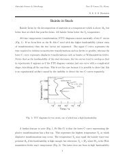
<strong>TTT</strong> diagrams<br />
<strong>TTT</strong> diagram stands for “time-temperature-transformation” diagram. It is<br />
also called isothermal transformation diagram<br />
Definition: <strong>TTT</strong> diagrams give the kinetics <strong>of</strong> isothermal<br />
transformations.<br />
2
Determination <strong>of</strong> <strong>TTT</strong> diagram for eutectoid steel<br />
Davenport and Bain were the first to develop the <strong>TTT</strong> diagram<br />
<strong>of</strong> eutectoid steel. They determined pearlite and bainite<br />
portions whereas Cohen later modified and included M S and<br />
M F temperatures for martensite. There are number <strong>of</strong> methods<br />
used to determine <strong>TTT</strong> diagrams. These are salt bath (Figs. 1-<br />
2) techniques combined with metallography and hardness<br />
measurement, dilatometry (Fig. 3), electrical resistivity<br />
method, magnetic permeability, in situ diffraction techniques<br />
(X-ray, neutron), acoustic emission, thermal measurement<br />
techniques, density measurement techniques and<br />
thermodynamic predictions. Salt bath technique combined<br />
with metallography and hardness measurements is the most<br />
popular and accurate method to determine <strong>TTT</strong> diagram.<br />
3
Fig. 1 : Salt bath I -austenitisation<br />
heat treatment.<br />
Fig. 2 : Bath II low-temperature<br />
salt-bath for isothermal treatment.<br />
4
Fig . 3(a): Sample and<br />
fixtures for dilatometric<br />
measurements<br />
Fig. 3(b) : Dilatometer<br />
equipment<br />
5
In molten salt bath technique two salt baths and one water<br />
bath are used. Salt bath I (Fig. 1) is maintained at austenetising<br />
temperature (780˚C for eutectoid steel). Salt bath II (Fig. 2) is<br />
maintained at specified temperature at which transformation is<br />
to be determined (below A e1), typically 700-250°C for<br />
eutectoid steel. Bath III which is a cold water bath is<br />
maintained at room temperature.<br />
In bath I number <strong>of</strong> samples are austenitised at A C1+20-40 C<br />
for eutectoid and hypereutectoid steel, A C3+20-40 C for<br />
hypoeutectoid steels for about an hour. Then samples are<br />
removed from bath I and put in bath II and each one is kept for<br />
different specified period <strong>of</strong> time say t 1, t 2, t 3, t 4, t n etc. After<br />
specified times, the samples are removed and quenched in<br />
water. The microstructure <strong>of</strong> each sample is studied using<br />
metallographic techniques. The type, as well as quantity <strong>of</strong><br />
phases, is determined on each sample.<br />
6
The time taken to 1% transformation to, say pearlite or bainite<br />
is considered as transformation start time and for 99%<br />
transformation represents transformation finish. On quenching<br />
in water austenite transforms to martensite.<br />
But below 230 C it appears that transformation is time<br />
independent, only function <strong>of</strong> temperature. Therefore after<br />
keeping in bath II for a few seconds it is heated to above<br />
230 C a few degrees so that initially transformed martensite<br />
gets tempered and gives some dark appearance in an optical<br />
microscope when etched with nital to distinguish from freshly<br />
formed martensite (white appearance in optical microscope).<br />
Followed by heating above 230 C samples are water<br />
quenched. So initially transformed martensite becomes dark in<br />
microstructure and remaining austenite transform to fresh<br />
martensite (white).<br />
7
Quantity <strong>of</strong> both dark and bright etching martensites are<br />
determined. Here again the temperature <strong>of</strong> bath II at which 1%<br />
dark martensite is formed upon heating a few degrees above<br />
that temperature (230 C for plain carbon eutectoid steel) is<br />
considered as the martensite start temperature (designated M S).<br />
The temperature <strong>of</strong> bath II at which 99 % martensite is formed<br />
is called martensite finish temperature ( M F).<br />
<strong>Transformation</strong> <strong>of</strong> austenite is plotted against temperature vs<br />
time on a logarithm scale to obtain the <strong>TTT</strong> diagram. The<br />
shape <strong>of</strong> diagram looks like either S or like C.<br />
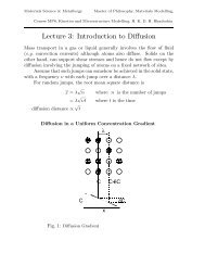
Fig. 4 shows the schematic <strong>TTT</strong> diagram for eutectoid plain<br />
carbon steel<br />
8
<strong>Temperature</strong><br />
% <strong>of</strong> Phase<br />
A e1<br />
T 2<br />
T 1<br />
Fig.4: <strong>Time</strong> temperature transformation (schematic) diagram for plain carbon<br />
eutectoid steel<br />
100<br />
0<br />
t 0<br />
t 1<br />
50%<br />
t2 t3 t4 t5 50% very fine pearlite + 50% upper bainite<br />
M S, Martensite start temperature<br />
M 50,50% Martensite<br />
T 1<br />
M F, Martensite finish temperature<br />
Log time<br />
Metastable austenite +martensite<br />
Martensite<br />
T 2<br />
Pearlite<br />
Fine pearlite<br />
Upper bainite<br />
Lower bainite<br />
Hardness<br />
At T 1, incubation<br />
period for pearlite=t 2,<br />
Pearlite finish time<br />
=t 4<br />
Minimum incubation<br />
period t 0 at the nose<br />
<strong>of</strong> the <strong>TTT</strong> diagram,<br />
M S=Martensite<br />
start temperature<br />
M 50=temperature<br />
for 50%<br />
martensite<br />
formation<br />
M F= martensite<br />
finish temperature<br />
9
At close to A e1 temperature, coarse pearlite forms at close to<br />
A e1 temperature due to low driving force or nucleation rate.<br />
At higher under coolings or lower temperature finer pearlite<br />
forms.<br />
At the nose <strong>of</strong> <strong>TTT</strong> diagram very fine pearlite forms<br />
Close to the eutectoid temperature, the undercooling is low so<br />
that the driving force for the transformation is small. However,<br />
as the undercooling increases transformation accelerates until<br />
the maximum rate is obtained at the “nose” <strong>of</strong> the curve.<br />
Below this temperature the driving force for transformation<br />
continues to increase but the reaction is now impeded by slow<br />
diffusion. This is why <strong>TTT</strong> curve takes on a “C” shape with<br />
most rapid overall transformation at some intermediate<br />
temperature.<br />
10
Pearlitic transformation is reconstructive. At a given temperature (say<br />
T 1) the transformation starts after an incubation period (t 2, at T 1).<br />
Locus <strong>of</strong> t 2 for different for different temperature is called<br />
transformation start line. After 50% transformation locus <strong>of</strong> that time<br />
(t 3 at T 1)for different temperatures is called 50% transformation line.<br />
While transformation completes that time (t 4 at T 1) is called<br />
transformation finish, locus <strong>of</strong> that is called transformation finish line.<br />
Therefore <strong>TTT</strong> diagram consists <strong>of</strong> different isopercentage lines <strong>of</strong><br />
which 1%, 50% and 99% transformation lines are shown in the<br />
diagram. At high temperature while underlooling is low form coarse<br />
pearlite. At the nose temperature fine pearlite and upper bainite form<br />
simultaneously though the mechanisms <strong>of</strong> their formation are entirely<br />
different. The nose is the result <strong>of</strong> superimposition <strong>of</strong> two<br />
transformation noses that can be shown schematically as below one<br />
for pearlitic reaction other for bainitic reaction (Fig. 6).<br />
Upper bainite forms at high temperature close to the nose <strong>of</strong> <strong>TTT</strong><br />
diagram while the lower bainite forms at lower temperature but above<br />
MS temperature.<br />
11
Fig. 5(a) : The appearance <strong>of</strong> a (coarse) pearlitic<br />
microstructure under optical microscope.<br />
12
Fig. 5(b): A cabbage filled with water analogy <strong>of</strong> the threedimensional<br />
structure <strong>of</strong> a single colony <strong>of</strong> pearlite, an<br />
interpenetrating bi-crystal <strong>of</strong> ferrite and cementite.<br />
13
Fig. 5(c): Optical micrograph showing colonies<br />
<strong>of</strong> pearlite . Courtesy <strong>of</strong> S. S. Babu.<br />
14
Fig. 5(d): Transmission electron micrograph<br />
<strong>of</strong> extremely fine pearlite.<br />
15
Fig. 5(e): Optical micrograph <strong>of</strong> extremely<br />
fine pearlite from the same sample as used to<br />
create Fig. 5(d). The individual lamellae<br />
cannot now be resolved.<br />
16
<strong>Temperature</strong><br />
Fig. 6: <strong>Time</strong> <strong>Temperature</strong> <strong>Transformation</strong> (schematic) diagram for plain carbon<br />
eutectoid steel<br />
A e1<br />
Metastable γ<br />
MS M50 MF γ<br />
Metastable γ + M<br />
M<br />
Log time<br />
P<br />
FP<br />
50% very FP + 50% UB<br />
UB<br />
LB<br />
Hardness<br />
γ=austenite<br />
α=ferrite<br />
CP=coarse pearlite<br />
P=pearlite<br />
FP=fine pearlite<br />
UB=upper bainite<br />
LB=lower bainite<br />
M=martensite<br />
M S=Martensite start<br />
temperature<br />
M 50=temperature for<br />
50% martensite<br />
formation<br />
M F= martensite finish<br />
temperature<br />
17
On cooling <strong>of</strong> metastable austenite 1% martensite forms at<br />
about 230°C. The transformation is athermal in nature. i.e.<br />
amount <strong>of</strong> transformation is time independent (characteristic<br />
amount <strong>of</strong> transformation completes in a very short time) but<br />
function <strong>of</strong> temperature alone. This temperature is called the<br />
martensite start temperature or M S.<br />
Below Ms while metastable austenite is quenched at different<br />
temperature amount <strong>of</strong> martensite increases with decreasing<br />
temperature and does not change with time.<br />
The temperature at which 99% martensite forms is called<br />
martensite finish temperature or M F. Hardness values are<br />
plotted on right Y-axis. Therefore a rough idea about<br />
mechanical properties can be guessed about the phase mix.<br />
18
<strong>TTT</strong> diagram gives<br />
Nature <strong>of</strong> transformation-isothermal or athermal (time<br />
independent) or mixed<br />
Type <strong>of</strong> transformation-reconstructive, or displacive<br />
Rate <strong>of</strong> transformation<br />
Stability <strong>of</strong> phases under isothermal transformation conditions<br />
<strong>Temperature</strong> or time required to start or finish transformation<br />
Qualitative information about size scale <strong>of</strong> product<br />
Hardness <strong>of</strong> transformed products<br />
19
Factors affecting <strong>TTT</strong> diagram<br />
Composition <strong>of</strong> steel-<br />
(a) carbon wt%,<br />
(b) alloying element wt%<br />
Grain size <strong>of</strong> austenite<br />
Heterogeneity <strong>of</strong> austenite<br />
Carbon wt%-<br />
As the carbon percentage increases A 3 decreases, similar is the case<br />
for A r3, i.e. austenite stabilises. So the incubation period for the<br />
austenite to pearlite increases i.e. the C curve moves to right. However<br />
after 0.77 wt%C any increase in C, A cm line goes up, i.e. austenite<br />
become less stable with respect to cementite precipitation. So<br />
transformation to pearlite becomes faster. Therefore C curve moves<br />
towards left after 0.77%C. The critical cooling rate required to prevent<br />
diffusional transformation increases with increasing or decreasing<br />
carbon percentage from 0.77%C and e for eutectoid steel is minimum.<br />
Similar is the behaviour for transformation finish time.<br />
20
Pearlite formation is preceeded by ferrite in case <strong>of</strong><br />
hypoeutectoid steel and by cementite in hypereutectoid steel.<br />
Schematic <strong>TTT</strong> diagrams for eutectoid, hypoeutectoid and<br />
hyper eutectoid steel are shown in Fig.4, Figs. 7(a)-(b) and all<br />
<strong>of</strong> them together along with schematic Fe-Fe 3C metastable<br />
equilibrium are shown in Fig. 8.<br />
21
<strong>Temperature</strong><br />
Fig. 7(a) :Schematic <strong>TTT</strong> diagram for plain carbon hypoeutectoid steel<br />
t 0<br />
A e3<br />
A e1<br />
Metastable γ<br />
MS M50 MF M<br />
FP + UB<br />
Log time<br />
Metastable γ + M<br />
α+CP<br />
α+P<br />
FP<br />
UB<br />
LB<br />
Hardness<br />
γ=austenite<br />
α=ferrite<br />
CP=coarse pearlite<br />
P=pearlite<br />
FP=fine pearlite<br />
UB=upper Bainite<br />
LB=lower Bainite<br />
M=martensite<br />
M S=Martensite start<br />
temperature<br />
M 50=temperature for<br />
50% martensite<br />
formation<br />
M F= martensite finish<br />
temperature<br />
22
<strong>Temperature</strong><br />
Fig. 7(b): Schematic <strong>TTT</strong> diagram for plain carbon hypereutectoid<br />
steel<br />
t 0<br />
A ecm<br />
A e1<br />
Metastable γ<br />
MS M50 very FP +UB<br />
Metastable γ + M<br />
Log time<br />
Fe 3C+CP<br />
Fe 3C+P<br />
Fe 3C+FP<br />
UB<br />
LB<br />
Hardness<br />
γ=austenite<br />
CP=coarse pearlite<br />
P=pearlite<br />
FP=fine pearlite<br />
UB=upper Bainite<br />
LB=lower Bainite<br />
M=martensite<br />
M S=Martensite start<br />
temperature<br />
M 50=temperature for<br />
50% martensite<br />
formation<br />
23
Fig. 8: Schematic Fe-Fe 3C metastable equilibrium diagram<br />
and <strong>TTT</strong> diagrams for plain carbon hypoeutectoid, eutectoid<br />
and hypereutectoid steels<br />
γ=austenite<br />
α=ferrite<br />
CP=coarse<br />
pearlite<br />
(a) Fe-Fe 3C<br />
metastable phase<br />
diagram<br />
M S<br />
P=pearlite<br />
FP=fine pearlite<br />
UB=upper bainite<br />
LB=lower bainite<br />
(b) <strong>TTT</strong> diagram for<br />
hypoeutectoid steel<br />
M=martensite<br />
M S=Martensite start temperature<br />
M 50=temperature for 50% martensite<br />
formation<br />
M F= martensite finish temperature<br />
(c ) <strong>TTT</strong> diagram<br />
for eutectoid steel<br />
(d) <strong>TTT</strong> diagram for<br />
hypereutectoid steel<br />
24
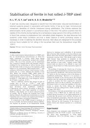
Under isothermal conditions for various compositions<br />
proeutectoid tranformation has been summarised below<br />
(Fig. 9). In hypoeutectoid steel the observable ferrite<br />
morphologies are grain boundary allotriomorph (α)(Fig.11(a)-<br />
(d)), Widmanstätten plate (α W)(Figs. 12-16), and massive (α M)<br />
ferrite (Fig.11(f)).<br />
Grain boundary allotriomorphs form at close to A e3<br />
temperature or extension <strong>of</strong> A ecm line at low undercooling.<br />
Widmanstätten plates form at higher undercooling but mainly<br />
bellow Ae 1. There are overlap regions where both<br />
allotriomorphs and Widmanstätten plates are observed.<br />
Equiaxed ferrite forms at lower carbon composition less than<br />
0.29 wt%C.<br />
25
<strong>Temperature</strong><br />
Fig 9: <strong>Temperature</strong> versus composition in which various morphologies<br />
are dominant at late reaction time under isothermal condition<br />
0.0218<br />
αM α W<br />
M F<br />
Lath martensite<br />
A e3<br />
A e1<br />
Austenite<br />
0.77<br />
Pearlite<br />
Mix martensite<br />
Upper bainite<br />
Lower bainite<br />
Weight % carbon<br />
M S<br />
Cm W<br />
Plate martensite<br />
Volume % <strong>of</strong> retained austenite<br />
W=Widmanstätten<br />
plate<br />
M=massive<br />
P=pearlite<br />
α ub=upper bainite<br />
α lb =lower bainite<br />
Volume % <strong>of</strong> retained<br />
austenite at room<br />
temperature<br />
26
There are overlapping regions where both equiaxed ferrite<br />
and Widmanstätten plates were observed. However at very low<br />
carbon percentage massive ferrite forms. The reconstructive<br />
and displacive mechanisms <strong>of</strong> various phase formation is<br />
shown in Fig. 10.<br />
In hypereutectoid steel both grain boundary allotriomorph and<br />
Widmanstatten plates were observed. Massive morphology<br />
was not observed in hypereutectoid steel. Grain boundary<br />
allotriomorphs were observed mainly close to A ecm or close to<br />
extension <strong>of</strong> A e3 line but Widmanstätten plates were observed<br />
at wider temperature range than that <strong>of</strong> hypoeutectoid steel. In<br />
hypereutectoid steel there are overlapping regions <strong>of</strong> grain<br />
boundary allotrioorph and Widmanstätten cementite.<br />
27
Fig. 10: The reconstructive and displacive mechanisms.<br />
28
Fig. 11(a): schematic diagram <strong>of</strong> grain boundary allotriomoph<br />
ferrite, and intragranular idiomorph ferrite.<br />
29
Fig.11(b): An allotriomorph <strong>of</strong> ferrite in a sample which is partially<br />
transformed into α and then quenched so that the remaining γ<br />
undergoes martensitic transformation. The allotriomorph grows<br />
rapidly along the austenite grain boundary (which is an easy diffusion<br />
path) but thickens more slowly.<br />
30
Fig. 11(c): Allotriomorphic ferrite in a Fe-0.4C steel which is<br />
slowly cooled; the remaining dark-etching microstructure is fine<br />
pearlite. Note that although some α-particles might be identified as<br />
idiomorphs, they could represent sections <strong>of</strong> allotriomorphs.<br />
Micrograph courtesy <strong>of</strong> the DoITPOMS project.<br />
31
Fig. 11(d): The allotriomorphs have in this slowly cooled lowcarbon<br />
steel have consumed most <strong>of</strong> the austenite before the<br />
remainder transforms into a small amount <strong>of</strong> pearlite.<br />
Micrograph courtesy <strong>of</strong> the DoItPoms project. The shape <strong>of</strong><br />
the ferrite is now determined by the impingement <strong>of</strong> particles<br />
32<br />
which grow from different nucleation sites.
Fig. 11(e): An idiomorph <strong>of</strong> ferrite in a sample which is partially<br />
transformed into α and then quenched so that the remaining γ<br />
undergoes martensitic transformation. The idiomorph is<br />
crystallographically facetted.<br />
33
Fig. 11(f ): Massive ferrite (α m) in Fe-0.002 wt%C alloy<br />
quenched into ice brine from 1000°C. Courtesy <strong>of</strong> T. B.<br />
Massalski<br />
34
Fig. 12(a): Schematic illustration <strong>of</strong> primary Widmanstätten<br />
ferrite which originates directly from the austenite grain<br />
surfaces, and secondary α w which grows from allotriomorphs.<br />
35
Fig. 12(b): Optical micrographs showing white-etching (nital)<br />
wedge-shaped Widmanstätten ferrite plates in a matrix quenched to<br />
martensite. The plates are coarse (notice the scale) and etch cleanly<br />
because they contain very little substructure.<br />
36
Fig. 13: The simultaneous growth <strong>of</strong> two selfaccommodating<br />
plates and the consequential tent-like<br />
surface relief.<br />
37
Fig.14: Transmission electron micrograph <strong>of</strong> what optically appears<br />
to be single plate, but is in fact two mutually accommodating plates<br />
with a low-angle grain boundary separating them. Fe-0.41C alloy,<br />
austenitised at 1200 C for 6 hrs, isothermally transformed at 700 C<br />
for 2 min and water quenched. 38
Fig. 15: Mixture <strong>of</strong> allotriomorphic ferrite, Widmanstätten ferrite<br />
and pearlite. Micrograph courtesy <strong>of</strong> DOITPOMS project.<br />
39
Fig. 16 (a) Surface relief <strong>of</strong> Widmanstätten ferrite Fe-0.41C<br />
alloy, austenitised at 1200 C for 6 hrs, isothermally<br />
transformed at 700 C for 30 min and water quenced, (b) same<br />
field after light polishing and etching with nital.<br />
40
For eutectoid steel banitic transformation occurs at 550 to<br />
250°C. At higher temperature it is upper bainite and at lower<br />
temperature it is lower bainite. As C increases the austenite to<br />
ferrite decomposition becomes increasingly difficult. As<br />
bainitic transformation proceeds by the nucleation <strong>of</strong> ferrite,<br />
therefore banitic transformation range moves to higher timing<br />
and lower temperature. With increasing percentage <strong>of</strong> carbon<br />
the amount <strong>of</strong> carbide in interlath region in upper bainite<br />
increases and carbides become continuous phase. However at<br />
lower percentage <strong>of</strong> carbon they are discrete particles and<br />
amount <strong>of</strong> carbide will be less in both type <strong>of</strong> bainites. For<br />
start and finish temperatures for both types <strong>of</strong> bainites go<br />
down significantly with increasing amount <strong>of</strong> carbon (Figs. 8-<br />
9). However increasing carbon makes it easier to form lower<br />
bainite.<br />
41
Fig 17: Summary <strong>of</strong> the mechanism <strong>of</strong> the bainite reaction.<br />
42
Fig. 18: Upper bainite; the<br />
phase between the platelets<br />
<strong>of</strong> bainitic ferrite is usually<br />
cementite.<br />
43
Fig. 19: Transmission electron micrograph <strong>of</strong> a sheaf <strong>of</strong> upper bainite in<br />
a partially transformed Fe-0.43C-2Si-3Mn wt% alloy (a) optical<br />
micrograph, (b, c) bright field and corresponding dark field image <strong>of</strong><br />
retained austenite between the sub units, (d) montage showing the<br />
44<br />
structure <strong>of</strong> the sheaf.
Fig. 20 : Corresponding outline <strong>of</strong> the sub-units near the sheaf tip<br />
region <strong>of</strong> Fig. 19 45
Fig. 21 : AFM image showing surface relief due to individual bainite<br />
subunit which all belong to tip <strong>of</strong> sheaf. The surface relief is<br />
associated with upper bainite (without any carbide ) formed at 350°C<br />
for 2000 s in an Fe-0.24C-2.18Si-2.32Mn-1.05Ni (wt% ) alloy<br />
austenitised at 1200°C for 120 s alloy. Both austenitisation and<br />
isothermal transformation were performed in vacuum. The<br />
microstructure contains only bainitic ferrite and retained austenite.<br />
The measured shear strain is 0.26±0.02.<br />
46
a b<br />
Fig. 22: Optical micrograph illustrating the sheaves <strong>of</strong> lower bainite in<br />
a partially transformed (395C), Fe-0.3C-4Cr wt% ally. The light<br />
etching matrix phase is martensite. (b) Corresponding transmission<br />
electron micrograph illustrating subunits <strong>of</strong> lower bainite.<br />
47
Fig. 23 : (a) Optical micrograph showing thin and spiny lower<br />
bainite formed at 190°C for 5 hours in an Fe-1.1 wt% C steel. (b)<br />
Transmission electron micrograph showing lower bainite midrib in<br />
same steel. Courtesy <strong>of</strong> M. Oka<br />
48
c<br />
d<br />
a<br />
b<br />
Fig. 24 : Schematic illustration <strong>of</strong><br />
various other morphologies: (a)<br />
Nodular bainite, (b) columnar bainite<br />
along a prior austenite boundary, (c)<br />
grain boundary allotriomorphic<br />
bainite, (d) inverse bainite<br />
49
Within the bainitic transformation temperature range, austenite <strong>of</strong><br />
large grain size with high inclusion density promotes acicular<br />
ferrite formation under isothermal transformation condition. The<br />
morphology is shown schematically (Figs. 25-27 )<br />
Fig. 25 : shows the morphology and nucleation site <strong>of</strong><br />
acicular ferrite.<br />
50
Fig . 26: Acicular ferrite<br />
51
Fig. 27: Replica transmission electron micrograph <strong>of</strong><br />
acicular ferrire plates in steel weld. Courtesy <strong>of</strong> Barritte.<br />
52
For eutectoid steel martensite forms at around 230°C. From<br />
230°C to room temperature martensite and retained austenite are<br />
seen. At room temperature about 6% retained austenite can be<br />
there along with martensite in eutectoid steel. At lower carbon<br />
percentage M S temperature goes up and at higher percentage M S<br />
temperature goes down (Fig. 4, Figs. 7-8, Fig. 28). Below 0.4<br />
%C there is no retained austenite at room but retained austenite<br />
can go up to more than 30% if carbon percentage is more than<br />
1.2%. Morphology <strong>of</strong> martensite also changes from lathe at low<br />
percentage <strong>of</strong> carbon to plate at higher percentage <strong>of</strong> carbon.<br />
Plate formation start at around 0.6 % C. Therefore below 0.6 %<br />
carbon only lathe martensite can be seen, mixed morphologies<br />
are observed between 0.6%C to 1%C and above 1% it is 100%<br />
plate martensite (Figs. 29-39).<br />
53
<strong>Temperature</strong><br />
Fig. 28: Effect <strong>of</strong> carbon on M S, M F temperatures and retained austenite in plain carbon<br />
steel<br />
A e3<br />
Ferrite + austenite<br />
0.0218<br />
Ferrite + pearlite<br />
M F<br />
Lath martensite<br />
A e1<br />
Austenite<br />
0.77<br />
Mix martensite<br />
Weight % carbon<br />
Pearlite<br />
M S<br />
Austenite +cementite<br />
Pearlite+cementite<br />
Volume % <strong>of</strong> retained<br />
austenite at room<br />
temperature<br />
Plate martensite<br />
Volume % <strong>of</strong> retained austenite<br />
54
Fig. 29: Morphology and crystallography <strong>of</strong> (bcc or bct) martensite in<br />
ferrous alloys<br />
Courtesy <strong>of</strong><br />
T. Maki<br />
Lath<br />
(Fe-9%Ni-0.15%C)<br />
Substructure Dislocation<br />
Habit plane<br />
{111} A<br />
{557} A<br />
O.R. K-S<br />
Lenticular<br />
(Fe-29%Ni-0.26%C)<br />
Dislocation<br />
Twin (midrib)<br />
{259} A<br />
{3 10 15} A<br />
N-W<br />
G-T<br />
Thin plate<br />
(Fe-31%Ni-0.23%C)<br />
Twin<br />
{3 10 15} A<br />
G-T<br />
Ms high low<br />
55
Fig. 30: Lath martensite<br />
Courtesy <strong>of</strong><br />
T. Maki<br />
56
Fig. 31: effect <strong>of</strong> carbon<br />
on martensite lath size<br />
Packet: a group <strong>of</strong> laths<br />
with the same habit plane<br />
( ~{111} )<br />
Block : a group <strong>of</strong> laths<br />
with the same orientation<br />
(the same K-S variant)<br />
(T. Maki,K. Tsuzaki, I. Tamura: Trans. ISIJ, 20(1980), 207.)<br />
57
Fig.32: Fe-29%Ni-0.26%C<br />
(Ms=203K)<br />
Fig. 33: Fe-31%Ni-0.28%C<br />
(Ms=192K)<br />
Lenticular martensite<br />
(Optical micrograph)<br />
Courtesy <strong>of</strong><br />
T. Maki<br />
Fig.34: schematic diagram for<br />
lenticular martensite<br />
58
Fig. 35: Growth behavior <strong>of</strong> lenticular martensite<br />
in Fe-30.4%Ni-0.4%C alloy<br />
cooling<br />
surface relief surface relief<br />
surface relief<br />
after polished and etched<br />
(T. Kakeshita, K. Shimizu, T. Maki, I. Tamura, Scripta Metall., 14(1980)1067.)<br />
Courtesy <strong>of</strong><br />
T. Maki<br />
59
Courtesy <strong>of</strong><br />
T. Maki<br />
Fig. 36: Lenticular martensite in Fe-33%Ni alloy<br />
(Ms=171K)<br />
Optical micrograph<br />
schematic illustration<br />
midrib twinned region<br />
60
Fig. 37: Optical microstructure <strong>of</strong> lath martensite (Fe-C alloys)<br />
0.0026%C 0.18%C<br />
0.38%C<br />
0.61%C<br />
Courtesy <strong>of</strong><br />
T. Maki<br />
61
Block structure in a single packet (Fe-0.18%C)<br />
Courtesy <strong>of</strong><br />
T. Maki<br />
Fig. 38: SEM image<br />
Fig.39 : Orientation<br />
image map
Alloying elements: Almost all alloying elements<br />
(except, Al, Co, Si) increases the stability <strong>of</strong> supercooled<br />
austenite and retard both proeutectoid and the pearlitic reaction<br />
and then shift <strong>TTT</strong> curves <strong>of</strong> start to finish to right or higher<br />
timing. This is due to i) low rate <strong>of</strong> diffusion <strong>of</strong> alloying<br />
elements in austenite as they are substitutional elements, ii)<br />
reduced rate <strong>of</strong> diffusion <strong>of</strong> carbon as carbide forming<br />
elements strongly hold them. iii) Alloyed solute reduce the rate<br />
<strong>of</strong> allotropic change, i.e. γ→α, by solute drag effect on γ→α<br />
interface boundary. Additionally those elements (Ni, Mn, Ru,<br />
Rh, Pd, Os, Ir, Pt, Cu, Zn, Au) that expand or stabilise<br />
austenite, depress the position <strong>of</strong> <strong>TTT</strong> curves to lower<br />
temperature. In contrast elements (Be, P, Ti, V, Mo, Cr, B, Ta,<br />
Nb, Zr) that favour the ferrite phase can raise the eutectoid<br />
temperature and <strong>TTT</strong> curves move upward to higher<br />
temperature.<br />
63
However Al, Co, and Si increase rate <strong>of</strong> nucleation and growth<br />
<strong>of</strong> both ferrite or pearlite and therefore shift <strong>TTT</strong> diagram to<br />
left. In addition under the complex diffusional effect <strong>of</strong> various<br />
alloying element the simple C shape behaviour <strong>of</strong> <strong>TTT</strong><br />
diagram get modified and various regions <strong>of</strong> transformation<br />
get clearly separated. There are separate pearlitic C curves,<br />
ferritic and bainitic C curves and shape <strong>of</strong> each <strong>of</strong> them are<br />
distinct and different.<br />
64
The effect <strong>of</strong> alloying elements is less pronounced in bainitic<br />
region as the diffusion <strong>of</strong> only carbon takes place (either to<br />
neighbouring austenite or within ferrite) in a very short time<br />
(within a few second) after supersaturated ferrite formation by<br />
shear during bainitic transformation and there is no need for<br />
redistribution <strong>of</strong> mostly substitutional alloying elements.<br />
Therefore bainitic region moves less to higher timing in<br />
comparison to proeutectoid/pearlitic region. Addition <strong>of</strong><br />
alloying elements lead to a greater separation <strong>of</strong> the reactions<br />
and result separate C-curves for pearlitic and bainitic regions<br />
(Fig. 40). Mo encourage bainitic reaction but addition <strong>of</strong> boron<br />
retard the ferrite reaction. By addition <strong>of</strong> B in low carbon Mo<br />
steel the bainitic region (almost unaffected by addition <strong>of</strong> B)<br />
can be separated from the ferritic region.<br />
65
<strong>Temperature</strong><br />
A e3<br />
A e1<br />
M S<br />
Fig. 40: Effect <strong>of</strong> boron on <strong>TTT</strong> diagram <strong>of</strong> low carbon Mo steel<br />
Metastable austenite<br />
Bainite start<br />
Ferrite C curve in low<br />
carbon Mo steel<br />
Addition <strong>of</strong> boron<br />
Metastable austenite + martensite<br />
Log time<br />
Bainite<br />
Ferrite C curve in low<br />
carbon Mo-B steel<br />
Pearlitic C curve in low<br />
carbon Mo steel Pearlitic C curve in low<br />
Addition <strong>of</strong> boron<br />
carbon Mo-B steel<br />
66
However bainitic reaction is suppressed by the addition <strong>of</strong> some<br />
alloying elements. B S temperature (empirical) has been given by<br />
Steven & Haynes<br />
B S( C)=830-270(%C)-90(%Mn)-37(%Ni)-70(%Cr)-83(%Mo)<br />
(elements by wt%)<br />
According to Leslie, B 50( C)=B S-60<br />
B F( C)=B S-120<br />
Most alloying elements which are soluble in austenite lower M S, M F<br />
temperature except Al, Co.<br />
Andrews gave best fit equation for M S:<br />
M S(°C)=539-423(%C)-30.4Mn-17.7Ni-12.1Cr-7.5Mo+10Co-7.5Si<br />
(concentration <strong>of</strong> elements are in wt%).<br />
Effect <strong>of</strong> alloying elements on M F is similar to that <strong>of</strong> M S. Therefore,<br />
subzero treatment is must for highly alloyed steels to transform<br />
retained austenite to martensite.<br />
67
<strong>Temperature</strong><br />
Addition <strong>of</strong> significant amount <strong>of</strong> Ni and Mn can change the nature <strong>of</strong><br />
martensitic transformation from athermal to isothermal (Fig. 41).<br />
Log time<br />
Fig. 41: kinetics <strong>of</strong> isothermal martensite in an Fe-Ni-Mn alloy 68
Effect <strong>of</strong> grain size <strong>of</strong> austenite: Fine grain size shifts S curve<br />
towards left side because it helps for nucleation <strong>of</strong> ferrite,<br />
cementite and bainite (Fig. 43). However Yang and Bhadeshia<br />
et al. have shown that martensite start temperature (M S) is<br />
lowered by reduction in austenite grain size (Fig. 42).<br />
Fig. 42: Suppression <strong>of</strong> Martensite<br />
start temperature as a function<br />
austenite grain size L γ. M O S is the<br />
highest temperature at which<br />
martensite can form in large<br />
austenite grain. M S is the observed<br />
martensite start temperature (at 0.01<br />
detectable fraction <strong>of</strong> martensite).<br />
Circles represent from low alloy data<br />
and crosses from high alloy data.<br />
69
T= M S. a, b are fitting empirial constants,<br />
m =average aspect ratio <strong>of</strong> martensite=0.05 assumed, V γ<br />
=average volume <strong>of</strong> austenite. f=detectable fraction <strong>of</strong><br />
martensite=0.01 (taken).<br />
It is expected similar effect <strong>of</strong> grain size on M F as on M S.<br />
Grain size <strong>of</strong> austenite affects the maximum plate or lath size.<br />
i.e. larger the austenite size the greater the maximum plate size<br />
or lath size<br />
70
<strong>Temperature</strong>, T<br />
Fig. 43 : Effect <strong>of</strong> austenite grain size on <strong>TTT</strong> diagram <strong>of</strong> plain carbon<br />
hypoeutectoid steel<br />
A e3<br />
A e1<br />
Metastable γ<br />
MS M50 MF For finer austenite<br />
M<br />
50% FP + 50% UB<br />
Metastable γ + M<br />
Log(time, t)<br />
α+CP<br />
α+P<br />
FP<br />
UB<br />
LB<br />
Hardness<br />
γ=austenite<br />
α=ferrite<br />
CP=coarse pearlite<br />
P=pearlite<br />
FP=fine pearlite<br />
UB=upper Bainite<br />
LB=lower Bainite<br />
M=martensite<br />
M S=Martensite start<br />
temperature<br />
M 50=temperature at<br />
which 50% martensite<br />
is obtained<br />
M F= martensite finish<br />
temperature<br />
71
Heterogeinity <strong>of</strong> austenite: Heterogenous austenite increases<br />
transformation time range, start to finish <strong>of</strong> ferritic, pearlitic<br />
and bainitic range as well as increases the transformation<br />
temperature range in case <strong>of</strong> martensitic transformation and<br />
bainitic transformation. Undissolved cementite, carbides act<br />
as powerful inocculant for pearlite transformation. Therefeore<br />
heterogeneity in austenite increases the transformation time<br />
range in diffussional transformation and temperature range <strong>of</strong><br />
shear transformation products in <strong>TTT</strong> diagram.<br />
72
• Martempering<br />
• Austempering<br />
• Isothermal Annealing<br />
• Patenting<br />
Applications <strong>of</strong> <strong>TTT</strong> diagrams<br />
Martempering : This heat treatment is given to oil hardenable<br />
and air hardenable steels and thin section <strong>of</strong> water hardenable<br />
steel sample to produce martensite with minimal differential<br />
thermal and transformation stress to avoid distortion and<br />
cracking. The steel should have reasonable incubation period<br />
at the nose <strong>of</strong> its <strong>TTT</strong> diagram and long bainitic bay. The<br />
sample is quenched above M S temperature in a salt bath to<br />
reduce thermal stress (instead <strong>of</strong> cooling below M F directly)<br />
(Fig. 44)<br />
73
Surface cooling rate is greater than at the centre. The cooling<br />
schedule is such that the cooling curves pass behind without<br />
touching the nose <strong>of</strong> the <strong>TTT</strong> diagram. The sample is<br />
isothermally hold at bainitic bay such that differential cooling<br />
rate at centre and surface become equalise after some time.<br />
The sample is allowed to cool by air through M S-M F such<br />
that martensite forms both at the surface and centre at the<br />
same time due to not much temperature difference and thereby<br />
avoid transformation stress because <strong>of</strong> volume expansion.<br />
The sample is given tempering treatment at suitable<br />
temperature.<br />
74
<strong>Temperature</strong><br />
Fig. 44: Martempering heatreatment superimposed on <strong>TTT</strong> diagram<br />
for plain carbon hypoeutectoid steel<br />
A e3<br />
A e1<br />
t 0<br />
M S<br />
M 50<br />
M F<br />
Martensite<br />
Log time<br />
50% FP + 50% UB<br />
Metastable γ Tempering<br />
Metastable γ + martensite<br />
α+CP<br />
α+P<br />
FP<br />
UB<br />
LB<br />
Tempered martensite<br />
γ=austenite<br />
α=ferrite<br />
CP=coarse pearlite<br />
P=pearlite<br />
FP=fine pearlite<br />
t 0=minimum incubation<br />
period<br />
UB=upper bainite<br />
LB=lower bainite<br />
M=martensite<br />
M S=Martensite start<br />
temperature<br />
M 50=temperature at which<br />
50% martensite is obtained<br />
M F= martensite finish<br />
temperature<br />
75
Austempering<br />
Austempering heat treatment is given to steel to produce lower<br />
bainite in high carbon steel without any distortion or cracking to<br />
the sample. The heat treatment is cooling <strong>of</strong> austenite rapidly in a<br />
bath maintained at lower bainitic temperature (above M s)<br />
temperature (avoiding the nose <strong>of</strong> the <strong>TTT</strong> diagram) and holding<br />
it here to equalise surface and centre temperature (Fig. 45) and .<br />
till bainitic finish time. At the end <strong>of</strong> bainitic reaction sample is<br />
air cooled. The microstructure contains fully lower bainite. This<br />
heat treatment is given to 0.5-1.2 wt%C steel and low alloy steel.<br />
The product hardness and strength are comparable to hardened<br />
and tempered martensite with improved ductility and toughness<br />
and uniform mechanical properties. Products donot required to<br />
be tempered.<br />
76
<strong>Temperature</strong><br />
Fig. 45: Austempering heatreatment superimposed on <strong>TTT</strong> diagram<br />
for plain carbon hypoeutectoid steel<br />
A e3<br />
A e1<br />
t 0<br />
M S<br />
M 50<br />
M F<br />
Metastable γ + martensite<br />
Martensite<br />
Log time<br />
50% FP + 50% UB<br />
Metastable γ Tempering<br />
α+CP<br />
α+P<br />
FP<br />
UB<br />
LB<br />
Lower bainite<br />
γ=austenite<br />
α=ferrite<br />
CP=coarse pearlite<br />
P=pearlite<br />
FP=fine pearlite<br />
t 0=minimum incubation<br />
period<br />
UB=upper bainite<br />
LB=lower bainite<br />
M=martensite<br />
M S=Martensite start<br />
temperature<br />
M 50=temperature at which<br />
50% martensite is obtained<br />
M F= martensite finish<br />
temperature<br />
77
Isothermal annealing<br />
• Isothermal annealing is given to plain carbon and alloy steels<br />
to produce uniform ferritic and pearlitic structures. The<br />
product after austenising taken directly to the annealing<br />
furnace maintained below lower critical temperature and hold<br />
isothermally till the pearlitic reaction completes (Fig. 46). The<br />
initial cooling <strong>of</strong> the products such that the temperature at the<br />
centre and surface <strong>of</strong> the material reach the annealing<br />
temperature before incubation period <strong>of</strong> ferrite. As the<br />
products are hold at constant temperature i.e. constant<br />
undercooling) the grain size <strong>of</strong> ferrite and interlamellar<br />
spacing <strong>of</strong> pearlite are uniform. Control on cooling after the<br />
end <strong>of</strong> pearlite reaction is not essential. The overall cycle time<br />
is lower than that required by full annealing.<br />
78
<strong>Temperature</strong><br />
Fig. 46: Isothermal annealing heat treatment superimposed on <strong>TTT</strong><br />
diagram <strong>of</strong> plain carbon hypoeutectoid steel<br />
M S<br />
M 50<br />
M F<br />
A e3<br />
t 0<br />
A e1<br />
Metastable γ<br />
Metastable γ + martensite<br />
Martensite<br />
Log time<br />
50% FP + 50% UB<br />
Ferrite and pearlite<br />
α+CP<br />
α+P<br />
FP<br />
UB<br />
LB<br />
γ=austenite<br />
α=ferrite<br />
CP=coarse pearlite<br />
P=pearlite<br />
FP=fine pearlite<br />
t 0=minimum incubation<br />
period<br />
UB=upper bainite<br />
LB=lower bainite<br />
M=martensite<br />
M S=Martensite start<br />
temperature<br />
M 50=temperature at which<br />
50% martensite is obtained<br />
M F= martensite finish<br />
temperature<br />
79
Patenting<br />
Patenting heat treatment is the isothermal annealing at the nose<br />
temperature <strong>of</strong> <strong>TTT</strong> diagram (Fig. 47). Followed by this the<br />
products are air cooled. This treatment is to produce fine<br />
pearlitic and upper bainitic structure for strong rope, spring<br />
products containing carbon percentage 0.45 %C to 1.0%C. The<br />
coiled ropes move through an austenitising furnace and enters<br />
the salt bath maintained at 550°C(nose temperature) at end <strong>of</strong><br />
salt bath it get recoiled again. The speed <strong>of</strong> wire and length <strong>of</strong><br />
furnace and salt bath such that the austenitisation get over<br />
when the wire reaches to the end <strong>of</strong> the furnace and the<br />
residency period in the bath is the time span at the nose <strong>of</strong> the<br />
<strong>TTT</strong> diagram. At the end <strong>of</strong> salt bath wire is cleaned by water<br />
jet and coiled.<br />
80
<strong>Temperature</strong><br />
Fig. 47: Patenting heat treatment superimposed on <strong>TTT</strong> diagram <strong>of</strong><br />
plain carbon hypoeutectoid steel<br />
M S<br />
M 50<br />
M F<br />
A e3<br />
t 0<br />
A e1<br />
Metastable γ<br />
Metastable γ + martensite<br />
Martensite<br />
Log time<br />
50% FP + 50% UB<br />
α+CP<br />
α+P<br />
FP<br />
UB<br />
LB<br />
fine pearlite and upper bainite<br />
γ=austenite<br />
α=ferrite<br />
CP=coarse pearlite<br />
P=pearlite<br />
FP=fine pearlite<br />
t 0=minimum incubation<br />
period<br />
UB=upper bainite<br />
LB=lower bainite<br />
M=martensite<br />
M S=Martensite start<br />
temperature<br />
M 50=temperature at which<br />
50% martensite is obtained<br />
M F= martensite finish<br />
temperature<br />
81
Prediction methods<br />
<strong>TTT</strong> diagrams can be predicted based on thermodynamic<br />
calculations.<br />
MAP_STEEL_MUCG83 program [transformation start<br />
curves for reconstructive and displacive transformations for<br />
low alloy steels, Bhadeshia et al.], was used for the following<br />
<strong>TTT</strong> curve <strong>of</strong> Fe-0.4 wt%C-2 wt% Mn alloy (Fig. 48)<br />
Fig. 48: Calculated<br />
transformation start curve<br />
under isothermal<br />
transformation condition<br />
82
The basis <strong>of</strong> calculating <strong>TTT</strong> diagram for ferrous sytem<br />
1. Calculation <strong>of</strong> A e3 <strong>Temperature</strong> below which ferrite<br />
formation become thermodynamically possible.<br />
2. Bainite start temperature B S below which bainite<br />
transformation occurs.<br />
3. Martensite start temperature M S below which martensite<br />
transformation occurs<br />
4. A set <strong>of</strong> C-curves for reconstructive<br />
transformation (allotriomorphic ferrite and pearlite).<br />
A set <strong>of</strong> C-curves for displacive<br />
transformations (Widmanstätten ferrite, bainite)<br />
A set <strong>of</strong> C-curves for fractional transformation<br />
5. Fraction <strong>of</strong> martensite as a function <strong>of</strong> temperature<br />
83
1. Calculation <strong>of</strong> A e3 temperature for multicomponent<br />
system. [Method adopted by Bhadeshia et al.]<br />
(This analysis is based on Kirkaldy and Barganis and is applicable for total alloying<br />
elements <strong>of</strong> less than 6wt% and Si is less than 1 wt%)<br />
General procedure <strong>of</strong> determination <strong>of</strong> phase boundary<br />
Assume T is the phase boundary temperature at which high<br />
temperature phase L is in equilibrium with low temperature phase γ.<br />
In case <strong>of</strong> pure iron then T is given by<br />
Where Xo is the mole fraction <strong>of</strong> iron then<br />
for A e3 temperature, low<br />
temperature phase γ to be<br />
substituted by α and high<br />
temperature phase L to be<br />
substituted by γ)<br />
Where X i=mole fraction <strong>of</strong> component i, γ i=activity coefficient <strong>of</strong> component i,<br />
R=universal gas constant, assuming 0 for Fe, 1for C, i=2 to n for Si, Mn, Ni,<br />
Cr, Mo, Cu,V, Nb, Co, W respectively.<br />
84
and 0 G L= standard Gibbs free energy <strong>of</strong> pure high temperature<br />
phase and 0 G γ= Standard Gibbs free energy <strong>of</strong> pure low<br />
temperature phase<br />
Similarly for carbon ( n=1) or component i<br />
The Wagner Taylor expansion for the activity coefficients<br />
are substituted in the above equations.<br />
85
The Wagner-Taylor expansions for activity coefficients are<br />
k=1 to 11 in this case<br />
Where =0 (assumed)<br />
are the Wagner interaction parameters i.e. interaction between<br />
solutes are negligible. The substitution <strong>of</strong> Wagner-Taylor<br />
expansions for activity coefficients gives temperature deviation<br />
∆T for the phase boundary temperature (due to the addition <strong>of</strong><br />
substitutional alloying elements<br />
86
In multicomponent system, the temperature deviations due to<br />
individual alloying additions are additive as long as solute<br />
solute interactions are negligible. Kirkaldy and co-workers<br />
found that this interaction are negiligible as long as total<br />
alloying additions are less than 6wt% and Si is less than<br />
1wt%].<br />
Eventually ∆T takes the following form<br />
Where To is the phase boundary<br />
temperature for pure Fe-C system and To<br />
is given by .<br />
87
And where<br />
for which<br />
and<br />
where n=1 or i and ∆°H o and ∆°H 1 are standard molar<br />
enthalpy changes corresponding to ∆°Go and ∆°G 1.<br />
88
If the relevant free energy changes ∆ o G and the interaction<br />
parameters ε are known then ∆T can be calculated for any<br />
alloy.<br />
Since all the thermodynamic functions used are dependent on<br />
temperature, ∆T cannot be obtained from single application<br />
<strong>of</strong> all values (used from various sources) but must be deduced<br />
iteratively. Initially T can be set as To, ∆T is calculated. Then<br />
T=T+ ∆T is used for T and ∆T is found. Iteration can be<br />
repeated for a few times (typically five times) about till T<br />
changes by less than 0.1K.<br />
This method obtains A e3 temperature with accuracy <strong>of</strong> ±10K.<br />
89
2. Bainite start temperature B S from Steven and Haynes formula<br />
B S( C)=830-270(%C)-90(%Mn)-37(%Ni)-70(%Cr)-83(%Mo)<br />
( % element by wt)<br />
Both bainite and Widmanstätten ferrite nucleate by same<br />
mechanism. The nucleus develops into Widmanstätten ferrite if<br />
at the transformation temperature the driving force available<br />
cannot sustain diffusionless transformation. By contrast bainite<br />
form from the same nucleus if the transformation can occur<br />
without diffusion. Therefore in principle B S=W S.<br />
Bainite transformation does not reach completion if austenite<br />
enriches with carbon. But in many steels carbide precipitation<br />
from austenite eliminates the enrichment and allow the<br />
austenite to transform completely. In those cases bainite finish<br />
temperature is given (according to Leslie) by<br />
90
At the M S temperature<br />
3. M S <strong>Temperature</strong>:<br />
91
In the above equation, T refers to M S temperature in absolute<br />
scale, R is universal gas constant, x=mole fraction <strong>of</strong> carbon,Yi is<br />
the atom fraction <strong>of</strong> the ith substitutional alloying element, ∆T magi<br />
and ∆T NMi are the displacement in temperature at which the free<br />
energy change accompanying the γ→α transformation in pure<br />
iron (i.e. ∆F Fe γ→α ) is evaluated in order to allow for the changes<br />
(per at%) due to alloying effects on the magnetic and nonmagnetic<br />
components <strong>of</strong> ∆F Fe γ→α , respectively. These values were<br />
taken from Aaronson, Zenner. ∆F Fe γ→α value was from Kaufmann.<br />
92
The other parameters are as follows<br />
(i) the partial molar heat <strong>of</strong> solution <strong>of</strong> carbon in ferrite,<br />
∆¯Hα=111918 J mol -1 (from Lobo) and<br />
∆¯Hα=35129+169105x J mol -1 (from Lobo)<br />
ii) the excess partial molar non-configurational entropy <strong>of</strong><br />
solution <strong>of</strong> carbon in ferrite ∆Sα=51.44 J mol -1 K -1 (from Lobo)<br />
∆Sγ=7.639+120.4x J mol -1 K -1 (from Lobo)<br />
ω α=the C-C interaction energy in ferrite=48570 J mol -1 (average<br />
value) (from Bhadeshia)<br />
ω γ=the corresponding C-C interaction energy in austenite values<br />
were derived , as a function <strong>of</strong> the concentrations <strong>of</strong> various<br />
alloying elements, using the procedure <strong>of</strong> Shiflet and Kingman<br />
and optimised activity data <strong>of</strong> Uhrenius. These results were<br />
plotted as a function <strong>of</strong> mole fraction <strong>of</strong> alloying elements and<br />
average interaction parameter ω¯ γ was calculated following<br />
Kinsman and Aaronson.<br />
93
∆f*=Zener ordering term was evaluated by Fisher.<br />
The remaining term, ∆F Fe γ→α’= free energy change from<br />
austenite to martensite as only function <strong>of</strong> carbon content.<br />
and is identical for Fe-C and Fe-C-Y steels as structure for<br />
both cases are identical (Calculated by Bhadeshia )=-900 to -<br />
1400 J mol -1 (for C 0.01 to 0.06 mole fraction, changes are not<br />
monotonic). However Lacher-Fowler-Guggenheim<br />
extrapolation gives better result <strong>of</strong> -1100 to -1400 J mol -1<br />
(Carbon mole fraction 0.01-0.06).<br />
The equation was solved iteratatively until the both sides <strong>of</strong><br />
the equation balanced with a residual error <strong>of</strong>
4. <strong>Transformation</strong> start and finish C curves<br />
The incubation period (τ) can be calculated from the following<br />
equation [Bhadeshia et al.]<br />
Where T is the isothermal transformation temperature in absolute<br />
scale, R is universal gas constant, Gmax is the maximum free energy<br />
change available for nucleation, Q is activation enthalpy for<br />
diffusion, C,p, z=20 are empirical constant obtained by fitting<br />
experimental data <strong>of</strong> T, Gmax, τ for each type <strong>of</strong> transformation<br />
(ferrite start, ferrite finish, bainite start and bainite finish) . By<br />
systematically varying p and plotting ln(τ Gp max/ Tz=20 ) against 1/RT<br />
for each type <strong>of</strong> transformation (reconstructive and displacive) till<br />
the linear regression coefficient R1 attains an optimum value. Once p<br />
has been determined Q and C follow from respectively the slope<br />
and intercept <strong>of</strong> the <strong>of</strong> plot. The same equation can be used to<br />
95<br />
predict transformation time.
Table-I: Chemical compositions, in wt% <strong>of</strong> the steel<br />
chosen to test the model<br />
96
The optimum values <strong>of</strong> p and corresponding values <strong>of</strong> C, Q for<br />
different types <strong>of</strong> steels (Table-I) where concentrations are in wt% are<br />
summarised below [Bhadeshia et.al.] (Table-II).<br />
Table-II: The optimum values <strong>of</strong> fitting constants<br />
FS=ferrite start, FF=ferrite finish, BS=bainite start and BF=bainite<br />
finish<br />
97
The bainite finish C-curve <strong>of</strong> the experimental <strong>TTT</strong> diagram<br />
not only shifts to longer time but also but is also shifts to<br />
lower temperature by about 120°C. Therefore this is taken<br />
care by plotting against in<br />
order to determine p, Q and C for the bainitic finish curve.<br />
Based on Q, C and Gmax value it can be predicted that Mo<br />
strongly retard the formation <strong>of</strong> ferrite through its large<br />
influence on Q. however it can promote bainite via the small<br />
negative coefficient that it has for the Q <strong>of</strong> the bainitic Ccurve.<br />
Cr retard both both bainite and ferrite but net effect is<br />
to promote the formation <strong>of</strong> bainite since the influence on the<br />
bainitic C-curve is relatively small. Ni has a slight retarding<br />
effect on tranformation rate. Mn has also retarding effect on<br />
ferrite as as well as bainitic transformation<br />
98
Fractional transformation curves<br />
Fractional transformation time can be estimated from the<br />
following Johnson-Mehl-Avrami equation.<br />
X=transformation volume fraction, K 1 is rate constant which is<br />
a function <strong>of</strong> temperature and austenite grain size d, n and m<br />
are empirical constants. By selecting steels <strong>of</strong> similar grain<br />
size, the austenite grain size can be neglected then the above<br />
equation simplifies to<br />
99
Assuming x=0.01 for transformation start and x=0.99 for<br />
transformation finish. For a given temperature transformation<br />
start time and finish time can be calculated then K 1 and n can<br />
be solved for each transformation product an a function <strong>of</strong><br />
temperature.<br />
Then fractional transformation curves for arbitary values <strong>of</strong> x<br />
can therefore be determined using<br />
100
Representation <strong>of</strong> intermediate state <strong>of</strong> transformation<br />
between 0% and 100% can be derived by fitting to the<br />
experimental <strong>TTT</strong> diagram as follows:<br />
Where x refers to the fraction <strong>of</strong> transformation.<br />
In most <strong>of</strong> <strong>TTT</strong> diagrams <strong>of</strong> Russell has a plateau at its<br />
highest temperature. Therefore a horizontal line can be drawn<br />
at B S and joining it to a C-curve calculated for temperatures<br />
below B S.<br />
101
Relation between observed and predicted values for ferrite start<br />
(FS), ferrite finish (FF), bainite start (BS) and bainite finish<br />
(BF) are shown in Fig. 49. Predicted value closely matches the<br />
observed values for selected low alloy steels. Predicted <strong>TTT</strong><br />
diagrams are projected on experimental diagrams (Figs. 50-52).<br />
The model correctly predicts bainite bay region in low alloy as<br />
well as in selected high alloy steels. The model reasonably<br />
predicts the fractional C curves (Fig. 52). Mo strongly retard the<br />
formation <strong>of</strong> ferrite through its large influence on Q. however it<br />
can promote bainite via the small negative coefficient that it<br />
has for the Q <strong>of</strong> the bainitic C-curve. Cr retard both both bainite<br />
and ferrite but net effect is to promote the formation <strong>of</strong> bainite<br />
since the influence on the bainitic C-curve is relatively small. Ni<br />
has a slight retarding effect on transformation rate. Mn has also<br />
retarding effect on ferrite as as well as bainitic transformation<br />
The model is impirical in nature but it can nevertheless be<br />
useful in procedure for the calculation <strong>of</strong> microstructure in steel.<br />
102
Fig. 49: Relation between observed and predicted Q(Jmol -1 )<br />
value for: (a) FS-ferrite start, (b) FF-ferrite finish, (c) BS-bainite<br />
start and (d) BF-bainite finish curves.<br />
103
Fig. 50: Comparison <strong>of</strong> experimental and predicted <strong>TTT</strong> diagram<br />
for BS steel:(a) En14, (b) En 16, (c) En 18 and (d) En 110.<br />
104
Fig. 51: Comparison <strong>of</strong> experimental and predicted <strong>TTT</strong> diagram for<br />
US steel:(a) US 4140, (b) US 4150, (c) US 4340 and (d) US 5150<br />
105
Fig. 52: Comparison <strong>of</strong> the experimental and predicted <strong>TTT</strong><br />
diagrams including fractional transformation curves at 0.1, 0.5<br />
and 0.9 transform fractions: (a)En 19 and (b) En24. 106
Limitations <strong>of</strong> model<br />
The model tends to overestimate the transformation time at<br />
temperature just below A e3. This is because the driving force<br />
term ∆G max is calculated on the basis <strong>of</strong> paraequilibrium and<br />
becomes zero at some temperature less than A e3 temperature.<br />
The coefficients utilized in the calculations were derived by<br />
fitting to experimental data, so that the model may not be<br />
suitable for extrapolation outside <strong>of</strong> that data set. Thus the<br />
calculation should be limited to the following concentration<br />
ranges (in wt%):C 0.15-0.6, Si 0.15-0.35, Mn 0.5-2.0, Ni 0-<br />
2.0, Mo 0-0.8 Cr 0-1.7.<br />
107
5. Fraction <strong>of</strong> martensite as a function <strong>of</strong> temperature<br />
Volume fraction <strong>of</strong> martensite formed at temperature T =f and<br />
f=1-exp[BVpdΔGv)/dT(M S-T)]<br />
Where, B=constant, Vp=volume <strong>of</strong> nucleus, ∆Gv=driving force<br />
for nucleation, M S =martensite start temperature. Putting the<br />
measured values<br />
the above equation becomes<br />
f=1-exp[-0.011(M S-T)] [Koistinen and Marburger equation].<br />
The above equation can be used to calculate the fraction <strong>of</strong><br />
martensite at various temperature.<br />
108