Absolute values of transport mean free path of light in non-absorbing ...
Absolute values of transport mean free path of light in non-absorbing ...
Absolute values of transport mean free path of light in non-absorbing ...

Create successful ePaper yourself
Turn your PDF publications into a flip-book with our unique Google optimized e-Paper software.
262 J. GALVAN-MIYOSHI AND R. CASTILLO<br />
where β is an <strong>in</strong>strumental factor determ<strong>in</strong>ed by collection<br />
optics. However, for microspheres mov<strong>in</strong>g <strong>in</strong> Brownian motion,<br />
� ∆r 2 (τ) � can also be evaluated us<strong>in</strong>g the E<strong>in</strong>ste<strong>in</strong> equation<br />
for hard-spheres corrected for concentration [13], i.e.,<br />
D = (kBT/6πηwa) � 1 − 1.83φ + 0.88φ 2� = � ∆r 2 (τ) � /6t,<br />
where ηw is the water viscosity, a is the microsphere radius,<br />
T is the temperature and kB is the Boltzmann constant. Then,<br />
us<strong>in</strong>g this � ∆r 2 (τ) � <strong>in</strong> Eq. 19 and the known <strong>values</strong> for a and<br />
L, we were able to calculate l ∗ as a <strong>free</strong> parameter fitt<strong>in</strong>g the<br />
experimental g1(τ) given <strong>in</strong> Eq. 19 for a DWS experiment.<br />
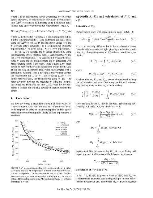
In Fig. 3, we <strong>in</strong>cluded the l ∗ <strong>values</strong> obta<strong>in</strong>ed by us<strong>in</strong>g<br />
the <strong>in</strong>tegrat<strong>in</strong>g sphere method, the Mie scatter<strong>in</strong>g theory, and<br />
the DWS measurements. The agreement between the measured<br />
l ∗ us<strong>in</strong>g the <strong>in</strong>tegrat<strong>in</strong>g sphere and l ∗ calculated with<br />
Mie scatter<strong>in</strong>g theory is excellent. There is just a 3.8% <strong>mean</strong><br />
deviation between theory and experiment, except for the case<br />
<strong>of</strong> the colloidal suspension made with microspheres with a<br />
diameter <strong>of</strong> 620 nm. This is because at this volume fraction<br />
the requirement that L ≫ l ∗ is not followed (L/l ∗ ∼ 8);<br />
<strong>in</strong> this particular case, the deviation was close to 12% . The<br />
<strong>mean</strong> deviation between the measured l ∗ us<strong>in</strong>g the <strong>in</strong>tegrat<strong>in</strong>g<br />
sphere and DWS was less than 2.5%. From these experiments,<br />
it is clear that we have developed a reliable method to<br />
obta<strong>in</strong> l ∗ .<br />
4. Conclusion<br />
We have developed a procedure to obta<strong>in</strong> absolute <strong>values</strong> <strong>of</strong><br />
l ∗ measur<strong>in</strong>g the static transmittance and reflectance <strong>of</strong> a colloidal<br />
suspension us<strong>in</strong>g an <strong>in</strong>tegrat<strong>in</strong>g sphere, and the agreement<br />
with <strong>values</strong> com<strong>in</strong>g from theory or from experiments is<br />
excellent.<br />
FIGURE 3. l ∗ for suspensions <strong>of</strong> polystyrene microspheres <strong>in</strong> water<br />
vs volume fraction. Microspheres <strong>of</strong> different diameters were used.<br />
Circles correspond to DWS measurements (see text), and triangles<br />
to measurements obta<strong>in</strong>ed us<strong>in</strong>g an <strong>in</strong>tegrat<strong>in</strong>g sphere. L<strong>in</strong>es were<br />
obta<strong>in</strong>ed from calculations us<strong>in</strong>g Mie scatter<strong>in</strong>g theory for spheres<br />
embedded <strong>in</strong> water.<br />
Appendix A. Ref and calculation <strong>of</strong> R(θ) and<br />
T (θ)<br />
Estimation <strong>of</strong> Ref<br />
Our derivation starts with expression 3.2 given <strong>in</strong> Ref. 14:<br />
J(θ) = v<br />
�<br />
U(0) + l<br />
2<br />
∗ cos θ ∂U<br />
∂z (0)<br />
�<br />
cos θ s<strong>in</strong> θ. (A.1)<br />
At z = L, the only diffusive flux <strong>in</strong> the −z direction comes<br />
from the effective reflected <strong>light</strong> given by a reflective coefficient<br />
Ref . Integrat<strong>in</strong>g along all θ for the +z semi-space, we<br />
obta<strong>in</strong>:<br />
where<br />
J−(L) = −<br />
�π<br />
π/2<br />
Ref (θ)J(θ)dθ, (A.2)<br />
Ref (θ) = R(θ) + RspTwbTwo(θ). (A.3)<br />
As shown below, Rsp and Twb, do not depend on θ, so they<br />
can be treated as constants. Cont<strong>in</strong>uity conditions for the energy<br />
density allow us to write, at the boundary:<br />
�<br />
v U0 l∗<br />
+<br />
2 2 3<br />
�<br />
∂U0<br />
= −<br />
∂z<br />
�π<br />
π/2<br />
Ref (θ)J(θ)dθ, (A.4)<br />
Here, the LHS is the J− flux <strong>in</strong> the bulk. Substitut<strong>in</strong>g J(θ)<br />
from Eq. A.1 <strong>in</strong> Eq. A.4, we obta<strong>in</strong> at z = L,<br />
with<br />
and<br />
Rev. Mex. Fís. 54 (3) (2008) 257–264<br />
U(L) + l ∗<br />
D1 =<br />
D2 =<br />
�π<br />
π/2<br />
�π<br />
π/2<br />
�<br />
1<br />
� 3<br />
1<br />
2<br />
�<br />
+ D2<br />
�<br />
+ D1<br />
∂U<br />
(L) = 0, (A.5)<br />
∂z<br />
Ref (θ) cos θ s<strong>in</strong> θdθ<br />
Ref (θ) cos 2 θ s<strong>in</strong> θdθ.<br />
Equation (A.5) is the same as Eq. (11) at z = L. Us<strong>in</strong>g both<br />
expressions we f<strong>in</strong>ally arrive at the follow<strong>in</strong>g expression:<br />
Ref = 3D2 − 2D1<br />
3D2 + 2D1 + 2 .<br />
Calculation <strong>of</strong> R(θ) and T (θ)<br />
In Eq. A.3, Ref (θ) is given <strong>in</strong> terms <strong>of</strong> R(θ) and Two(θ).<br />
Both terms are estimated consider<strong>in</strong>g multiple <strong>in</strong>ternal reflections<br />
at the cell wall [10] as shown <strong>in</strong> Fig. 4. Each reflectance