Absolute values of transport mean free path of light in non-absorbing ...

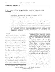
INSTRUMENTACIÓN REVISTA MEXICANA DE FÍSICA 54 (3) 257–264 JUNIO 2008
Absolute values of transport mean free path of light in non-absorbing media using
transmission and reflectance measurements
J. Galvan-Miyoshi and R. Castillo*
Instituto de Física, Universidad Nacional Autónoma de Mexico,
P.O. Box 20-364, Mexico, 01000 D.F.
Recibido el 19 de febrero de 2008; aceptado el 23 de abril de 2008
We derived a relation between the transport mean free path of light, and transmittance and the reflectance in non-absorbing turbid media.
This allowed us to develop an experimental procedure to obtain absolute values for the transport mean free path of light just by measuring
in an integrating sphere both the transmittance and the reflectance in this kind of system. We determined how accurate our method was by
comparing our transport mean free path measurements with calculations made for colloidal suspensions of particles using Mie scattering
theory and with measurements made in colloidal suspensions of polystyrene microspheres using diffusive wave spectroscopy. The agreement
is excellent.
Keywords: Transport mean free path of light; DWS.
En este trabajo se deriva una relación entre el camino libre medio de trasporte de la luz y la transmitancia y la reflectancia de un medio
turbio no absorbente. Esto nos permitió desarrollar un procedimiento experimental para obtener valores absolutos de los caminos libes
medio de transporte de la luz con sólo medir, en una esfera integradora, la trasnmitancia y la reflectancia en esta clase de sistemas. Hemos
determinado cuán preciso es nuestro método comparando nuestras medidas de camino libre medio de transporte con cálculos efectuados para
suspensiones coloidales utilizando la teoría de dispersión de Mie y con medidas hechas en suspensiones coloidales de microesferas utilizando
espectroscopia de onda difusa. El acuerdo es excelente.
Descriptores: Camino libre medio de trasporte de luz; DWS.
PACS: 82.70.Dd; 87.64Cc; 78.20.Ci
1. Introduction
Light scattering techniques had been widely used in several
fields to extract dynamical and structural information in complex
fluids. Initially, these techniques were limited to transparent
samples, where single scattering is a good approximation.
However, in the past fifteen years, new developments
made it possible to take into account multiple scattering,
leading to diffusive wave spectroscopy (DWS) [1]. This
technique extends the single scattering experiment to multiple
scattering assuming that light transport in the sample can
be treated as a diffusive process. Using DWS, it is possible
to measure the mean square displacement, 〈∆r 2 (t)〉, of
embedded colloidal particles in a fluid, which makes it possible
to obtain the response of viscoelastic materials to shear
excitations through the complex shear modulus, G ∗ (ω). This
modulus determines the stress induced on a material upon application
of an oscillatory shear strain at a frequency ω. Normally,
G ∗ (ω) is determined using mechanical rheometers,
where viscoelastic properties are measured by application of
strain, while measuring stress or vice versa. This bulk mechanical
susceptibility G ∗ (ω) also determines the response
of colloidal particles embedded in a fluid. These probe particles,
excited by thermal stochastic forces, move in Brownian
motion along the fluid. [2, 3] 〈∆r 2 (t)〉 can be related
to G ∗ (w) by describing the motion of particles with a generalized
Langevin equation incorporating a memory function
to take into account the viscoelasticity of the fluid where the
particles are embedded. In this way, the particle fluctuation
spectrum can be used to measure the relaxation spectrum of
the fluid. With DWS, there is no strain applied to the material
during the measurement. This is a useful characteristic for
complex fluids where even small imposed strains can cause
structural reorganization of the material and can change its
viscoelastic properties.
In a DWS experiment, a laser beam strikes a slab formed
by a turbid suspension made of the liquid under study and
probe colloidal particles that scatter light. The temporal autocorrelation
function of a small fraction of the light that
passes through the slab is measured. The transport of light
through the slab is treated as a diffusive process and photons
are treated as random walkers, with a random walk step
length equal to the transport mean free path l ∗ and a resultant
diffusion coefficient D = vl ∗ /3, where v is the speed of
light in the suspension. The diffusion approximation is valid
for calculating transport of light only over distances much
longer than l ∗ [1]. When scattering is not isotropic, which is
the case for particle sizes close to and larger than the photon
wavelength, the random walk step length is longer than the
photon mean free path length l. These lengths are connected
by l ∗ /l = 2k 2 o/ � q 2� , where ko = 2πn/λ is the photon wave
vector in the solvent, λ is the laser wavelength in a vacuum,
n is the effective index of refraction in the sample, and � q 2�
represents the average angle for the squared scattering vector
for a typical scattering event experienced by the photon in the
medium.
l ∗ is a key parameter that enters into the DWS analysis
and has to be determined independently. It is usually mea-

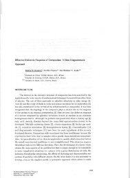
258 J. GALVAN-MIYOSHI AND R. CASTILLO
sured by comparing the system transmittance with that of
calibrated suspensions of latex spheres in water where l ∗ is
known [1,4,5]. There are just a few experimental procedures
to determine l ∗ without using a reference sample. Mitani
et al. [6] used coherent backscattering, Weitz and Pine [1]
used pulsed DWS where l ∗ is estimated by measuring the delay
time of a signal due to the multiple scattering. Garcia
et al. [7] developed a procedure where microwave radiation
power is measured in the forward scattering geometry, using
boundary conditions so that reflected waves from an integrating
cavity can be neglected.
In this paper, we present a procedure to obtain absolute
values of the transport mean free path of light in
non-absorbing media made of a colloidal suspension of
polystyrene microspheres. In this procedure, the basic issue
is to measure the transmission and the reflectance of the
colloidal suspension under study using an integrating sphere.
We determined how accurate our method was by comparing
our results with calculations made for colloidal suspensions
of particles using Mie scattering theory and with experimental
measurements made in colloidal suspensions using diffusive
wave spectroscopy. The agreement is excellent.
1.1. Transport mean free path
In this section, we present the basic equations to obtain l ∗
from transmittance and reflectance measurements carried out
in turbid non-absorbing samples made of colloidal particles
dispersed in a fluid, using an integrating sphere as shown in
Fig. 1. The system is contained in a rectangular cell with parallel
windows. Here, a collimated light of power P 0 is sent
to an integrating sphere with an internal Lambertian surface.
Light is collected by a detector placed on the wall of the integrating
sphere, in the following conditions: one with no sample
at entrance and reflectance ports (beam striking directly
on the sphere wall), one in transmission geometry (sample at
entrance port, shown in Fig. 1) and one in reflection geometry
(sample at reflection port). As we shall show from these
measurements, by taking into account the transmission and
reflectance of the cell walls, it is possible to obtain reliable
values of l ∗ .
FIGURE 1. Schematic diagram of the integrating sphere with an
amplification showing the light transmittances along the cell walls
and sample, from outside to the integrating sphere.
1.1.1. Transmittance and reflectance of a fluid sample obtained
using an integrating sphere
To obtain the transmittance T ∗ of a turbid colloidal suspension,
we need to analyze the transmission and reflection of
light when the suspension is placed in two different configurations:
at the entrance port and at the reflection port of an
integrating sphere. The transmitted or the reflected light from
the sample is multiply reflected by the surface of the integrating
sphere before reaching the detector. The collected light
is a function of the incident power and of the geometric and
reflection parameters of the sphere. Pickering et al. [8, 9]
studied just this problem, so we shall use their derivation to
obtain some of our working equations. For transmittance, the
, is given by:
collected power at the detector, P T d
P T d = δ
A
�
mAeff Tcd
1 − [r δ
A + mAeff + Rd(s ′′ /A)]
�
P 0T . (1)
When the sample is in reflection geometry, light first strikes
the integrating sphere, thus, diffuse light irradiates the sample.
The collected power, P R d , at the detector can be expressed
as:
�
�
m
P 0R . (2)
P R d = δ
A
1 − [r δ
A + mAeff + Rd(s ′ /A)]
In these equations, P 0T and P 0R are the incident powers, δ
is the area of the detector, m is the reflection factor of the
sphere wall, Rd is the diffuse reflection factor of the sample
for diffuse incident light, s ′′ and s ′ are the areas of the
transmission and reflection ports, respectively. A is the total
area of the sphere, Tcd is the diffusive transmission factor of
the sample for collimated incident light (sample including the
cell walls), Aeff = 1 − (δ/A + d/A + h/A) is the area fraction
of the sphere wall relative to the total sphere area, h is
the area of the sphere open holes, and d is s ′′ or s ′ depending
on the measurement type. A baffle between the entrance port
and the detector was considered and the term rδ/A was not
neglected as it was in Pickering et al. [8]. Equations 1 and 2
can be rewritten in the following manner:
and
where
and
Rev. Mex. Fís. 54 (3) (2008) 257–264
P T d = b Aeff Tcd
P
1 − cRd
0T , (3)
1
P R d = b
1 − cRd(s ′ /s ′′ )] P 0R , (4)
b = δ
�
m
A 1 − � r δ
�
�
A + mAeff
c = s′′
�
1
A 1 − � r δ
�
� .
A + mAeff

ABSOLUTE VALUES OF TRANSPORT MEAN FREE PATH OF LIGHT IN NON-ABSORBING MEDIA. . . 259
Solving for Tcd in Eq. 3 and substituting Rd using Eq. 4, we
obtain the following equation:
Tcd = 1
bAeff
�
1 − s′′
s ′
�
1 − b
0R P
P R �� T Pd . (5)
d P 0T
If collimated light, P 0 , is allowed to enter the sphere directly,
striking the sphere wall, in a geometry where there is no sample
in any port (Rd = 0), we find using Eq. 4, that P 0 0
d = bP
and
Tcd = 1
�
1 −
Aeff
s′′
s ′
�
1 − P 0 d
P R �� T Pd d P 0 . (6)
d
Therefore, if the same incident light is used in all cases,
P 0 = P 0R = P 0T , Eq. 6 allows us to obtain, Tcd in just one
experiment by measuring P 0 d , P T d and P R d , i.e., the power as
measured with the detector at the sphere wall when there is no
sample, in transmission geometry and in reflection geometry,
respectively.
Some final considerations need to be mentioned, because
Tcd is the total transmittance through the sample and also
through the cell walls. We need the transmittance through just
the colloidal suspension alone. Therefore, a correction has to
be made. Observing Fig. 1, transmittances along the optical
path in the sample are related as Tcd = T1T ∗ T0, where T0 is
the transmittance of the first cell wall in the path followed by
the light beam. It can be obtained from Fresnel coefficients
at normal incidence, producing
T0 =
16m13
(m12 + 1) 2 (m23 + 1)
2 ≈ 0.95,
where mij = ni/nj and ni are the refractive indices for
air (1), cell wall (2), and sample (3). T1 is the transmittance
for diffusive light coming from the sample through the exit
cell wall to the sphere. T1 can be approximated by considering
multiple reflections for an infinite non-absorbing slab
with a transmittance given by T∞ = 1 − R∞. Now, we
shall consider an approximation where the ratio of the finite
size transverse window reflectance to the infinite slab reflectance
is an expression equal to the ratio used for the transmittance,
i.e., T0/T∞ ≈ R/R∞, since the index of refraction
for microemulsions and cell wall are very close. Then,
T0 ≈ (R/R∞)(1 − R∞). An expression for calculating R
will be given below in Eq. 16. Finally, using this correction
T ∗ , the actual transmittance just through the colloidal suspension
can be calculated and related to l ∗ as shown in the
following paragraph.
1.1.2. Equations relating T ∗ with l ∗
In this section, a derivation to obtain a relation between T ∗
and l ∗ is presented. The suspension sample is considered a
slab of infinite transverse extent and thickness L, placed in a
static transmission geometry at the front port of an integrating
sphere as shown in Fig. 1. Here, laser light is coming
into the sample from z < 0 direction and some diffuse light
passes through the sample. Some light is transmitted to the
integrating sphere and some diffuse light is reflected back to
the sample. In this configuration, the static transmission coefficient
can be calculated within the photon diffusion approximation,
modifying the procedure used by Pine et al. [3] and
by Kaplan et al. [10].
The transmission coefficient for the sample can be calculated
using the diffusion approximation by dividing the transmitted
flux by the total flux:
T ∗ =
|J+(L)|
, (7)
|J+(L)| + |J−(0)|
where J± are the fluxes for the diffusing photons in the +z
and −z directions. In the absence of absorption, the photon
transport is described by the photon energy density U. Solving
the steady-state one-dimensional diffusion equation for
the photon energy density U(z), we obtain
�
Al + Blz, z < zo
U(z) =
, (8)
Ar + Brz, z ≥ zo
where zo = α ∗ l ∗ , and α ∗ ≈ 1. The solution U(z) must be
continuous at zo [10]; therefore,
Al + Blzo = Ar + Brzo. (9)
To define the boundary conditions for the onedimensional
diffusion equation, the net flux on the sample
must be considered. At z = 0, J+(0) = −RJ−(0). Nevertheless,
at z = L, it is necessary to take into account the
diffused light transmitted from the sample to the integrating
sphere and reflected back to the sample. Actually, this
is the difference between our derivation and Eq. A8 given in
Ref.10. We consider two contributions for the J−(L) calculation:
the light reflected at the cell wall, RJ+(L), and the fraction
of light reflected back from the integrating sphere. The
last term comprises the light going from the sample through
the cell wall, TwoJ+, then reflected back from the integrating
sphere, Rsp(TwoJ+), and re-entering the sample through the
cell wall with a transmission coefficient Twb(Rsp(TwoJ+)).
Then, the net calculation produces the actual reflection coefficient:
Ref = R + TwoRspTwb. (10)
The boundary condition for the sample at z = L is:
J−(L) = Ref J+(L) = (R + TwoRspTwb) J+(L).
The explicit expressions for
J− = v
�
U(0)
2 2
and
Rev. Mex. Fís. 54 (3) (2008) 257–264
l∗ ∂U
+
3 ∂z (0)
�
J+ = − v
�
U(0) l∗ ∂U
−
2 2 3 ∂z (0)
�
can be used with the boundary conditions at z = 0 and z = L,
to obtain [10]:
U(0) − C0
∂U
(0) = 0
∂z

260 J. GALVAN-MIYOSHI AND R. CASTILLO
and
where
U(L) + CL
C0 = 2 (1 + R)
3 (1 − R)
∂U
(L) = 0, (11)
∂z
and CL = 2 (1 + Ref )
3 (1 − Ref ) .
Now, using Eqs. 8, 9, and J± expressions, we obtain the
following expressions for the fluxes:
J−(0) = v Al
2 C0l∗ �
C0l∗ �
l∗
+ =
2 3
vAl
(3C0 + 2) , (12)
12C0
and
∗ vAll
J+(L) = −
12C0
(C0 + α∗ ) (3CL + 2)
(L + CLl∗ , (13)
− zo)
JT = |J−(0)| + |J+(L)| = vAl
12C0
�
(3C0+2) (y+CL−α
×
∗ ) + (C0+α∗ ) (3CL+2)
(y+CL−α∗ �
, (14)
)
where y = L/l ∗ . Finally, the static transmission coefficient
is given by:
T ∗ =
(C0+α ∗ ) (3CL+2)
(3C0+2) (y+CL−α ∗ ) + (C0+α ∗ ) (3CL+2)
. (15)
This final expression for T ∗ depends on α ∗ , L, and l ∗ as well
as on R and on Ref through C0 and CL. As we shall show
below, all variables involved in this equation can be measured
to obtain l ∗ . α ∗ can be obtained through a backscattering experiment,
as described in Appendix C, while R is calculated
with the procedure given by Kaplan et al. [10], using:
l ∗ =
This expression is our basic working equation to obtain l ∗
from experimental data.
2. Experimental section
Materials. Polystyrene microspheres (Bangs Labs Inc,
USA) of different diameters were used to prepare the water
suspensions and also functioned as microsphere tracers in the
DWS experiments to measure l ∗ . Glass cells were supplied
by Hellma GmbH (Germany) and by Starna Cells Inc (USA)
with different optical paths (2 mm to 4 mm) and different
cross sections (3.0 × 4.2 mm and 2.8 × 3.7 mm). Water was
milli-Q water (Nanopure-UV, USA; 18.3MΩ). Microspheres
were added to water while stirring. Water suspensions were
usually prepared with volume fractions < 0.04.
Integrating sphere throughput. An integrating sphere
(Oriel Newport, USA) was used to obtain l ∗ in the colloidal
suspensions. Here, light detection was carried out by a photo
multiplier tube (Hamamatsu Ltd, Japan) attached at the wall
sphere. We obtained the integrating sphere throughput by
where
and
R = 3C2 + 2C1
. (16)
3C2 − 2C1 + 2
�
C1 =
π/2
0
�
C2 =
π/2
0
R(θ) cos θ sin θdθ
R(θ) cos 2 θ sin θdθ.
Ref can be calculated using the procedure presented in Appendix
A, where the following formula is obtained:
with
and
D1 = −C1 + RspTwb
D2 = C2 + RspTwb
Ref = 3D2 − 2D1
, (17)
3D2 + 2D1 + 2
�π
π/2
�π
π/2
Two(θ) cos θ sin θdθ,
Two(θ) cos 2 θ sin θdθ.
Finally, solving for l ∗ in Eq. 15 and taking into account the
transmittance along the wall cells, we obtain:
(3C0 + 2) TcdL
(C0 + α ∗ ) (3CL + 2) (T1T0 − Tcd) + (CL − α ∗ ) (3C0 + 2) Tcd
. (18)
measuring the incident power, P 0 , at the front entrance port
of the integrating sphere, and then maintaining the laser light
power; constant the light power at the detection port of the
integrating sphere, P 0 d
Rev. Mex. Fís. 54 (3) (2008) 257–264
, was measured. The throughput is
b = P 0 d /P 0 . The integrating sphere is part of the instrument
described below.
Transport mean free path, l ∗ . We measured transmittance
and reflectance for the suspensions under study with an
integrating sphere as shown in Figs. 1 and 2, where a laser
beam (λ = 514.5 nm) expanded and collimated with a 2
mm pinhole was sent at normal incidence into the entrance
port of the sphere. To measure l ∗ , we followed Eq. (18),
where the total transmittance Tcd for a sample-cell system
was measured, as described in Eq. (6), using the light power
collected by the sphere detector in three different cases: when
the sample is placed at the entrance port (transmission geom-
), when it is placed at the reflection port (reflection
etry, P T d
geometry, P R d ), and when there is no sample on any port, P 0 d .

ABSOLUTE VALUES OF TRANSPORT MEAN FREE PATH OF LIGHT IN NON-ABSORBING MEDIA. . . 261
FIGURE 2. Schematic diagram of the DWS instrument. A laser beam is sent through a filter and a beam expander (BE). The beam is
deviated by a mirror (M) depending on the experiment. In the case of l ∗ measurements, the beam is sent into the sample and the scattered
light is collected by an integrating sphere. In the case of DWS measurements, the beam is sent into the sample (S) that is in a temperature
controlled bath (TB). The scattered light is collected, with the aid of an achromatic doublet (AD) and a beam splitter (BS), by a couple of
photomultipliers in cross correlation and by a CCD camera to make multispeckle DWS.
Instrument. The integrating sphere is included in a
home-made instrument shown schematically in Fig. 2, which
is mainly used to make DWS measurements. A laser beam
(Coherent Innova 300, Coherent Inc, USA) is filtered and
subsequently expanded to avoid sample heating and to ensure
the plane wave approximation. The beam is sent at
normal incidence onto a square cell where the colloidal suspensions
made with microspheres that multiply scatter light
are placed. The scattered light is collected by photomultiplier
tubes (Thorn EMI, England) through polarizing maintaining
optical fibers from OZoptics Inc (USA). Signals are
converted into TTL pulses using ALV preamplifiers (ALV
GmbH, Germany) and processed by an ALV/5000E multitau
correlator (ALV GmbH, Germany) to obtain the intensity
ACFs; most of our work was done in transmission geometry.
3. Results and Discussion
We determined l ∗ for different colloidal water suspensions
with the method described in the experimental section. We
also determined how accurate our method is for obtaining l ∗ ,
comparing our results with other, both theoretical and experimental
ones ways to obtain l ∗ .
In Fig. 3, we present the results of our l ∗ measurements
for water suspensions of latex microspheres at different concentrations
using the integrating sphere method that employs
Eq. (18); the sizes of the dispersed microspheres were also
varied. As may be observed, l ∗ decreases as 1/φ for the explored
concentration range, where φ is the volume fraction.
From Eq. (B.1) in Appendix B, a necessary consequence
of this concentration dependence is that the structure factor
S(q) ∼ 1 indicates that the interaction among microsphere
particles is negligible. The dependence of l∗ on particle diameter
between 250 and 800 nm is not simple, as previously
shown by [4].
To assess the quality of our l∗ measurements for colloidal
suspensions with microspheres with different sizes, we calculated
l∗ using Mie scattering theory following the procedures
developed by several authors [5, 11, 12] and described
in Appendix B. Also, we measured l∗ using DWS in transmission
geometry for suspensions where the properties of the
particles are known. Here, the field autocorrelation function
g1(τ), was obtained for water suspensions made of particles
with a known diameter and refractive index (nmic = 1.59
at 514.5 nm), at different particle concentration. g1(τ) is related
to the � ∆r2 (τ) � of the particles through the fundamental
working equation in DWS [1]:
L/l ∗ +4/3 �
∗ 2
sinh [α x] +
g1(τ) =
α∗ +2/3
�
4 1 + 9x2� sinh � L
l∗ x � + 4
3x cosh � L
l∗ x
3 x cosh [α∗ x] �
� (19)
This equation is valid for the transmission of a plane wave
through a slab of thickness L � l∗ and infinite transverse extent,
made of the scattering particles immersed in the liquid.
x = [k 2 o
Rev. Mex. Fís. 54 (3) (2008) 257–264
� ∆r 2 (τ) � ] 1/2 and α ∗ = zo/l ∗ ; zo is the distance into
the sample from the incident surface to the place where the
diffuse source is located. Therefore, measuring the intensity
correlation function g2(τ) allows us to obtain g1(τ) through
the Siegert relation:
g (2)(τ)t = 1 + β � �
�g �
(1)(τ)t
2 ,

262 J. GALVAN-MIYOSHI AND R. CASTILLO
where β is an instrumental factor determined by collection
optics. However, for microspheres moving in Brownian motion,
� ∆r 2 (τ) � can also be evaluated using the Einstein equation
for hard-spheres corrected for concentration [13], i.e.,
D = (kBT/6πηwa) � 1 − 1.83φ + 0.88φ 2� = � ∆r 2 (τ) � /6t,
where ηw is the water viscosity, a is the microsphere radius,
T is the temperature and kB is the Boltzmann constant. Then,
using this � ∆r 2 (τ) � in Eq. 19 and the known values for a and
L, we were able to calculate l ∗ as a free parameter fitting the
experimental g1(τ) given in Eq. 19 for a DWS experiment.
In Fig. 3, we included the l ∗ values obtained by using
the integrating sphere method, the Mie scattering theory, and
the DWS measurements. The agreement between the measured
l ∗ using the integrating sphere and l ∗ calculated with
Mie scattering theory is excellent. There is just a 3.8% mean
deviation between theory and experiment, except for the case
of the colloidal suspension made with microspheres with a
diameter of 620 nm. This is because at this volume fraction
the requirement that L ≫ l ∗ is not followed (L/l ∗ ∼ 8);
in this particular case, the deviation was close to 12% . The
mean deviation between the measured l ∗ using the integrating
sphere and DWS was less than 2.5%. From these experiments,
it is clear that we have developed a reliable method to
obtain l ∗ .
4. Conclusion
We have developed a procedure to obtain absolute values of
l ∗ measuring the static transmittance and reflectance of a colloidal
suspension using an integrating sphere, and the agreement
with values coming from theory or from experiments is
excellent.
FIGURE 3. l ∗ for suspensions of polystyrene microspheres in water
vs volume fraction. Microspheres of different diameters were used.
Circles correspond to DWS measurements (see text), and triangles
to measurements obtained using an integrating sphere. Lines were
obtained from calculations using Mie scattering theory for spheres
embedded in water.
Appendix A. Ref and calculation of R(θ) and
T (θ)
Estimation of Ref
Our derivation starts with expression 3.2 given in Ref. 14:
J(θ) = v
�
U(0) + l
2
∗ cos θ ∂U
∂z (0)
�
cos θ sin θ. (A.1)
At z = L, the only diffusive flux in the −z direction comes
from the effective reflected light given by a reflective coefficient
Ref . Integrating along all θ for the +z semi-space, we
obtain:
where
J−(L) = −
�π
π/2
Ref (θ)J(θ)dθ, (A.2)
Ref (θ) = R(θ) + RspTwbTwo(θ). (A.3)
As shown below, Rsp and Twb, do not depend on θ, so they
can be treated as constants. Continuity conditions for the energy
density allow us to write, at the boundary:
�
v U0 l∗
+
2 2 3
�
∂U0
= −
∂z
�π
π/2
Ref (θ)J(θ)dθ, (A.4)
Here, the LHS is the J− flux in the bulk. Substituting J(θ)
from Eq. A.1 in Eq. A.4, we obtain at z = L,
with
and
Rev. Mex. Fís. 54 (3) (2008) 257–264
U(L) + l ∗
D1 =
D2 =
�π
π/2
�π
π/2
�
1
� 3
1
2
�
+ D2
�
+ D1
∂U
(L) = 0, (A.5)
∂z
Ref (θ) cos θ sin θdθ
Ref (θ) cos 2 θ sin θdθ.
Equation (A.5) is the same as Eq. (11) at z = L. Using both
expressions we finally arrive at the following expression:
Ref = 3D2 − 2D1
3D2 + 2D1 + 2 .
Calculation of R(θ) and T (θ)
In Eq. A.3, Ref (θ) is given in terms of R(θ) and Two(θ).
Both terms are estimated considering multiple internal reflections
at the cell wall [10] as shown in Fig. 4. Each reflectance

ABSOLUTE VALUES OF TRANSPORT MEAN FREE PATH OF LIGHT IN NON-ABSORBING MEDIA. . . 263
and transmittance is calculated using Fresnel’s law [10, 14].
The total reflectance due to the cell wall is given by:
R(θ1) = R12(θ1)
+ T12(θ1)R23(θ2)T21(θ2)
× 1 − (R21(θ2)R23(θ2)) N+1
1 − R21(θ2)R23(θ2)
(A.6)
and the total transmittance through the cell wall is given by:
T13(θ1) = T12(θ1)T23(θ2)
× 1 − (R21(θ2)R23(θ2)) N+1
, (A.7)
1 − R21(θ2)R23(θ2)
where R12(θ1), T12(θ1), R23(θ2) and T21(θ2) are the reflectances
and transmittances at the sample-wall(12) and
wall-air (23) interfaces, and
� � � �
D/2 D
N = =
,
h 4d tan θ2
with D the height and d the thickness of the cell walls. N is
included as a cutoff due to the finiteness of the cell transversal
extension.
Twb
Now, the transmittance through the cell wall, from the integrating
sphere back to the sample, can be obtained using
FIGURE 4. Diagram showing reflection and transmission emerging
beams form the sample at the cell wall. θ1, θ2, and θ3 are the
incident angle, transmitted in the cell, and angle transmitted out of
the cell, respectively. n1, n2, and n3 are the refraction indices for
the water, cell wall and air, respectively. d is the cell wall thickness
and D is the sample cell height; beyond this distance multiple
reflections are not taken into account.
Eq.(A.7) but now with θ3 as the incident angle and considering
the transmittance from media 3 through media 1.
Twb(θ3) = T32(θ3)T21(θ2)
N+1
1 − (R21(θ2)R23(θ2))
.
1 − R21(θ2)R23(θ2)
If no preferred direction of incidence is assumed, the total
transmittance is calculated by integrating over all angles with
a constant probability distribution. Therefore:
Twb = 1
2π
�2π
0
�
π
π/2
Twb(θ) cos(θ) sin(θ)dθdφ, (A.8)
which does not depend on the angular distribution of J±.
Rsp
Rsp is the fraction of light that enters the integrating sphere
and returns to the cell wall. This can be estimated in the same
way as in Pickering et al. [8]. Light entering the integrating
sphere from the sample is reflected many times onto the integrating
sphere, detector and sample; also some of the light
escapes through the empty ports. Taking this into consideration,
the total fraction of light incident on the cell wall is
Rsp = s′′
δ b P T d
P 0T , (A.9)
d
where b is a constant for the sphere in the geometry used.
Appendix B. l ∗ from Mie and Percus-Yevick
Transport mean free path, l ∗ , is related to the mean free path
by [1]:
l ∗ ≡
l
〈1 − cos θ〉 =
1
,
ρ 〈1 − cos θ〉 σsca
where θ is the scattering angle, 〈〉 is the average over all scattering
angles, ρ = φ/(4πa 3 /3) the number density and
σsca = 2π
k 4 o
�
2ko
0
P (q)S(q)qdq
is the scattering cross section [15] for multiple scattering in
the far field. Here, P (q) = k 2 0(dσsca/dΩ) [11,12] is the Mie
scattering function for a single sphere, S(q) is the static structure
function., and q = 2k0 sin(θ/2) is the scattering vector
magnitude. We can write l ∗ as
l ∗ =
where we have used
Rev. Mex. Fís. 54 (3) (2008) 257–264
k 6 o
2k 2 0 〈1 − cos θ〉 = � q 2� =
πρ � 2ko
0 P (q)S(q)q3 , (B.1)
dq
2ko �
P (q)S(q)q
0
3dq .
2ko �
P (q)S(q)qdq
0

264 J. GALVAN-MIYOSHI AND R. CASTILLO
If P (q) and S(q) are known, l ∗ can be determined using
Eq. (B.1). To give an estimate, we calculated P (q) with Mie
theory for a non-absorbing spherical particle immersed in a
non-absorbing medium using:
with
P (θ) = k 2 �
oσdiff (θ) = π |S1 (θ)| 2 + |S2 (θ)| 2�
,
S1 (θ) =
S2 (θ) =
∞�
n=1
∞�
n=1
(2n + 1)
n (n + 1)
× [anπn (cos θ) + bnτn (cos θ)] , (B.2)
(2n + 1)
n (n + 1)
× [anτn (cos θ) + bnπn (cos θ)] . (B.3)
Here, τn (cos θ) = (d/dθ)P 1 n (cos θ) and
πn (cos θ) = P 1 n (cos θ)
,
sin θ
with P 1 n (cos θ) the Legendre polynomials, and an and bn coefficients
determined by the boundary conditions.
S(q) can be calculated for a system of hard spheres using
Percus-Yevick closure [16], which gives:
∗. Author to whom correspondence should be addressed: e-mail:
rolandoc@fisica.unam.mx
1. D.A. Weitz, D.J. Pine in: Dynamic Light Scattering, W. Brown
(Ed.). (Oxford University Press, New York, 1993) Chap. 16, p.
652.
2. J.L. Harden and V. Viasnoff, Curr. Opin. Colloid. Interface Sci.
6 (2001) 438.
3. D.J. Pine, D.A. Weitz, P.M. Chaikin, and E. Herbolzheimer,
Phys. Rev. Lett. 60 (1988) 1134.
4. F. Scheffold, J. Dispersion Sci. and Technol. 23 (2002) 591.
5. L.F. Rojas-Ochoa, D. Lacoste, R. Lenke, P. Schurtenberger, and
F. Scheffold, J. Opt. Soc. Am.A. 21 (2004) 1799.
6. S. Mitani, K. Sakai, and K. Takagi, Jpn. J. Appl. Phys. 39
(2000) 146.
7. N. Garcia, A.Z. Genack, and A.A. Lisyansky, Phys. Rev. B. 46
(1992) 14475.
1
S(q)
p1
= 1 + sin (2q) − 2q cos(2q)
q3 − p2
q3 �� �
1
− 2 q cos(2q) + 2 sin(2q) −
q2 1
�
q
�
3
+ φp1
2q 3
− φp1
2q 3
�
2
+ 4
q3 �
where p1 = 3φ(1+2φ)2
(1−φ) 4
Rev. Mex. Fís. 54 (3) (2008) 257–264
�
1 − 3
2q 2
1 − 3 3
+
q2 2q4 and p2 = (3φ)2
2
Appendix C. Estimation of α ∗
� �
sin(2q)
� �
q cos(2q) , (B.4)
(2+φ) 2
(1−φ) 4 .
α ∗ = zo/l ∗ can be estimated using a DWS experiment by fitting
the intensity autocorrelation function for the back scattered
light from a colloidal suspension made of particles of
the same size as those to be used in the fluid to be investi-
gated [4], using the expression:
�
(g2(t) − 1) pol = β exp
−2γpol
� �
6t
. (C.1)
τ
Here, the subscript pol is used to indicate the polarization detection
used in the experiment, V V for parallel and V H for
cross polarization. Here, τ = � k2 oD �−1 is the relaxation time
and D is the diffusion coefficient, and γpol = α∗ pol + 2/3. As
D is known, α∗ ≡ 〈α∗ 〉 = (α∗ V V + α∗ V H ) /2 can be determined
from a fitting.
8. J.W. Pickering, C.J.M. Moes, H.J.C.M. Sterenborg, S.A. Prahl,
and M.J.C. van Gemert, J. Opt. Soc. Am. A 9 (1992) 621.
9. J.W. Pickering, S.A. Prahl, N. van Wieringen, J.F. Beek,
H.J.C.M. Sterenborg, and M.J.C. van Gemert, App. Opt. 32
(1993) 399.
10. P.D. Kaplan, M.H. Kao, A.G. Yodh, and D.J. Pine, Appl. Opt.
32 (1993) 3828.
11. A. Ishimaru, Wave Propagation and Scattering in Random Media
(Academic Press, New York, 1978).
12. H.C. van de Hulst. Light Scattering by Small Particles (Dover,
New York, 1981).
13. G.K. Batchelor, J. Fluid Mech. 74 (1976) 1.
14. J.X. Zhu, D.J. Pine, D.A. Weitz, Phys. Rev. A 44 (1991) 3948.
15. L.F. Rojas-Ochoa, S. Romer, F. Scheffold, and P. Schurtenberger,
Phys. Rev. E. 65 (2002) 051403.
16. M.S. Wertheim, Phys. Rev. Lett. 10 (1963) 321.