IUCN Red List Guidelines - The IUCN Red List of Threatened Species

Guidelines for Using the IUCN Red List
Categories and Criteria
Version 9.0 (September 2011)
Prepared by the Standards and Petitions Subcommittee
of the IUCN Species Survival Commission.
Citation: IUCN Standards and Petitions Subcommittee. 2011. Guidelines for Using the IUCN
Red List Categories and Criteria. Version 9.0. Prepared by the Standards and Petitions
Subcommittee. Downloadable from
http://www.iucnredlist.org/documents/RedListGuidelines.pdf.

Contents
1. INTRODUCTION ..................................................................................................................................... 4
2. AN OUTLINE OF THE RED LIST CATEGORIES AND CRITERIA ............................................... 4
2.1 TAXONOMIC LEVEL AND SCOPE OF THE CATEGORIZATION PROCESS ......................................................... 4
2.1.1 Taxonomic scale of categorization ................................................................................................ 4
2.1.2 Geographical scale of categorization ........................................................................................... 6
2.1.3 Introduced taxa ............................................................................................................................. 7
2.2 NATURE OF THE CATEGORIES ................................................................................................................... 7
2.2.1 Transfer between categories ....................................................................................................... 10
2.3 NATURE OF THE CRITERIA ...................................................................................................................... 12
2.4 CONSERVATION PRIORITIES AND ACTIONS .............................................................................................. 15
2.5 DOCUMENTATION .................................................................................................................................. 15
3. DATA QUALITY .................................................................................................................................... 15
3.1 DATA AVAILABILITY, INFERENCE AND PROJECTION ................................................................................ 15
3.2 UNCERTAINTY ....................................................................................................................................... 17
3.2.1 Types of uncertainty .................................................................................................................... 17
3.2.2 Representing uncertainty ............................................................................................................ 17
3.2.3 Dispute tolerance and risk tolerance .......................................................................................... 18
3.2.4 Dealing with uncertainty ............................................................................................................. 18
3.2.5 Documenting uncertainty and interpreting listings ..................................................................... 18
3.2.6 Uncertainty and the application of the categories Data Deficient and Near Threatened ........... 19
4. GUIDELINES FOR THE DEFINITIONS OF TERMS USED IN THE CRITERIA ........................ 19
4.1 POPULATION AND POPULATION SIZE (CRITERIA A, C AND D) ................................................................. 19
4.2 SUBPOPULATIONS (CRITERIA B AND C) .................................................................................................. 19
4.3 MATURE INDIVIDUALS (CRITERIA A, B, C AND D).................................................................................. 20
4.3.1 Notes on defining mature individuals.......................................................................................... 20
4.3.2 Colonial or modular organisms .................................................................................................. 21
4.3.3 Fishes .......................................................................................................................................... 22
4.3.4 Sex-changing organisms ............................................................................................................. 22
4.3.5 Trees ............................................................................................................................................ 23
4.4 GENERATION (CRITERIA A, C1 AND E) ................................................................................................... 23
4.5 REDUCTION (CRITERION A) .................................................................................................................... 25
4.5.1 Estimating reduction ................................................................................................................... 25
4.5.2 Inferring or projecting population reduction .............................................................................. 26
4.6 CONTINUING DECLINE (CRITERIA B AND C) ........................................................................................... 26
4.7 EXTREME FLUCTUATIONS (CRITERIA B AND C2) .................................................................................... 28
4.8 SEVERELY FRAGMENTED (CRITERION B)................................................................................................ 30
4.9 EXTENT OF OCCURRENCE (CRITERIA A AND B) ...................................................................................... 31
4.10 AREA OF OCCUPANCY (CRITERIA A, B AND D) ....................................................................................... 34
4.10.1 Problems of scale ................................................................................................................... 35
4.10.2 Methods for estimating AOO .................................................................................................. 35
4.10.3 The appropriate scale ............................................................................................................. 36
4.10.4 Scale-area relationships ......................................................................................................... 36
4.10.5 Scale correction factors .......................................................................................................... 37
4.10.6 "Linear" habitat ..................................................................................................................... 39
4.10.7 AOO based on habitat maps and models ............................................................................... 40
4.11 LOCATION (CRITERIA B AND D) ............................................................................................................. 41
4.12 QUANTITATIVE ANALYSIS (CRITERION E) ............................................................................................... 42
5. GUIDELINES FOR APPLYING CRITERION A ............................................................................... 42
5.1 THE USE OF TIME CAPS IN CRITERION A ................................................................................................. 44
5.2 HOW TO APPLY CRITERION A4 ............................................................................................................... 45
5.3 THE SKI-JUMP EFFECT ............................................................................................................................ 45
5.4 SEVERELY DEPLETED POPULATIONS ....................................................................................................... 46
5.5 FISHERIES .............................................................................................................................................. 46
5.6 TREES .................................................................................................................................................... 46
5.7 RELATIONSHIP BETWEEN LOSS OF HABITAT AND POPULATION REDUCTION ............................................. 47

Red List Guidelines 3
5.8 TAXA WITH WIDELY DISTRIBUTED OR MULTIPLE POPULATIONS ........................................................... 48
5.8.1 Estimating reduction ................................................................................................................... 49
5.8.2 Dealing with uncertainty ............................................................................................................. 52
6. GUIDELINES FOR APPLYING CRITERION B ................................................................................ 57
7. GUIDELINES FOR APPLYING CRITERION C ............................................................................... 57
8. GUIDELINES FOR APPLYING CRITERION D ............................................................................... 58
8.1 TAXA KNOWN ONLY FROM THE TYPE LOCALITY ..................................................................................... 59
8.2 EXAMPLE OF APPLYING CRITERION D ..................................................................................................... 59
8.3 EXAMPLE OF APPLYING CRITERION D2 ................................................................................................... 59
9. GUIDELINES FOR APPLYING CRITERION E ................................................................................ 59
9.1 WHAT IS EXTINCTION? ........................................................................................................................... 60
9.2 WHICH METHOD CAN BE USED? ............................................................................................................. 60
9.3 ARE THERE SUFFICIENT DATA?............................................................................................................... 61
9.4 MODEL COMPONENTS AND PARAMETERS ............................................................................................... 62
9.4.1 Density dependence ..................................................................................................................... 62
9.4.2 Temporal variability.................................................................................................................... 62
9.4.3 Spatial variability ........................................................................................................................ 63
9.5 INCORPORATING UNCERTAINTY ............................................................................................................. 63
9.6 DOCUMENTATION REQUIREMENTS ......................................................................................................... 63
10. GUIDELINES FOR APPLYING THE CATEGORIES DD, NT AND NE ........................................ 64
10.1 WHEN TO USE THE CATEGORY NEAR THREATENED ............................................................................... 64
10.2 NOT EVALUATED AND DATA DEFICIENT ................................................................................................ 65
10.3 WHEN TO USE DATA DEFICIENT ............................................................................................................. 65
11. GUIDELINES FOR APPLYING THE EXTINCT CATEGORIES AND TAG ................................ 67
11.1 THE EXTINCT CATEGORIES (EX AND EW).............................................................................................. 67
11.2 ‘POSSIBLY EXTINCT’ TAG FOR CRITICALLY ENDANGERED TAXA ........................................................... 68
11.2.1 Identifying Possibly Extinct species ....................................................................................... 68
11.2.2 Examples of Critically Endangered (Possibly Extinct) species .............................................. 69
12. GUIDELINES FOR THREATENING PROCESSES .......................................................................... 71
12.1 GLOBAL CLIMATE CHANGE .................................................................................................................... 71
12.1.1 Time horizons ......................................................................................................................... 71
12.1.2 Definition of "Location" under climate change ..................................................................... 73
12.1.3 Inferring population reduction and continuing decline from results of bioclimatic models .. 74
12.1.4 Using criterion D2.................................................................................................................. 75
12.1.5 Severe fragmentation .............................................................................................................. 76
12.1.6 Extreme fluctuations ............................................................................................................... 77
12.1.7 Criterion E .............................................................................................................................. 77
12.1.8 Using bioclimate models ........................................................................................................ 78
13. REFERENCES ........................................................................................................................................ 82
14. APPENDIX: SUMMARY OF CHANGES TO THE GUIDELINES .................................................. 87

Red List Guidelines 4
1. Introduction
The IUCN Red List Categories and Criteria were first published in 1994 following six years
of research and broad consultation (IUCN 1994). The 1994 IUCN Categories and Criteria
were developed to improve objectivity and transparency in assessing the conservation status
of species, and therefore to improve consistency and understanding among users. The 1994
categories and criteria were applied to a large number of species in compiling the 1996 Red
List of Threatened Animals. The assessment of many species for the 1996 Red List drew
attention to certain areas of difficulty, which led IUCN to initiate a review of the 1994
categories and criteria, which was undertaken during 1998 to 1999. This review was
completed and the IUCN Red List Categories and Criteria (version 3.1) are now published
(IUCN 2001).
This document provides guidelines to the application of version 3.1 of the categories and
criteria, and in so doing addresses many of the issues raised in the process of reviewing the
1994 categories and criteria. This document explains how the criteria should be applied to
determine whether a taxon belongs in a category of threat, and gives examples from different
taxonomic groups to illustrate the application of the criteria. These guidelines also provide
detailed explanations of the definitions of the many terms used in the criteria. The guidelines
should be used in conjunction with the official IUCN Red List Categories and Criteria
booklet (IUCN 2001).
We expect to review and update these guidelines periodically, and input from all users of the
IUCN Red List Categories and Criteria are welcome. We especially welcome IUCN
Specialist Groups and Red List Authorities to submit examples that are illustrative of these
guidelines. We expect that the changes to these guidelines will be mostly additions of detail
and not changes in substance. In addition, we do not expect the IUCN Red List Criteria to be
revised in the near future, because a stable system is necessary to allow comparisons over
time.
2. An Outline of the Red List Categories and Criteria
2.1 Taxonomic level and scope of the categorization process
2.1.1 Taxonomic scale of categorization
The criteria may be applied to any taxonomic unit at or below the species level. In these
guidelines, the terms ‘taxon’ and ‘taxa’ are used to represent species or lower taxonomic
levels, including forms that are not yet fully described. There is sufficient range among the
different criteria to enable appropriate listing of taxa from the complete taxonomic spectrum,
with the exception of micro-organisms. In presenting the results of applying criteria, the
taxonomic unit used (species, subspecies, etc.) should be specified. It should be noted that
taxa below the rank of variety (e.g., forma, morph, cultivar), are NOT included on the IUCN
Red List, with the exception of assessments of subpopulations. Before assessments of taxa
below the species level (subspecies, variety or subpopulation) can be included on the IUCN
Red List, an assessment of the full species is also required.

Red List Guidelines 5
Subpopulations: If a subpopulation assessed under the criteria is not isolated (i.e., if it may
be exchanging individuals with other subpopulations), its assessments must follow the
regional guidelines (IUCN 2003). In addition, it must be a biological subpopulation (i.e., not
defined by political or national boundaries). Although the regional guidelines can in
principle be applied at any geographical scale, application within very small geographical
areas is strongly discouraged. The smaller the subpopulation as a proportion of the global
population of the species, the more often the subpopulation will exchange individuals with
other subpopulations. Therefore the assessment of extinction risk based on the criteria
would become more unreliable (IUCN 2003). See also Geographical scale of categorization
below.
Newly described species: The inclusion of newly described species on the IUCN Red List is
addressed on a case-by-case basis. The designated IUCN Red List Authority and/or IUCN
Global Species Programme staff (including staff from partner institutions working on Global
Species Assessment projects) will consult with relevant experts to ascertain how widely
accepted these are.
Undescribed species: The listing of undescribed species on the IUCN Red List is
discouraged, but in exceptional circumstances these may be included. There must be a clear
conservation benefit to justify the inclusion of such listings, or in the case of projects to
completely assess a taxonomic group, undescribed species that are listed as Least Concern
(LC) or Data Deficient (DD) may only be included if there is clear evidence that work is
underway to describe the species concerned and that the new species will be widely accepted.
The new species description should be published within four years of an undescribed species
being included on the IUCN Red List; if it is not published or is not in press after that time,
the assessment will be removed. For an undescribed species to be included on the IUCN Red
List the following conditions must be met:
• There must be general agreement that the undescribed form is a clearly circumscribed
species
• There must be a clear indication that work is underway to describe the species (e.g., a
draft manuscript in preparation or a paper with the new description already submitted
for publication)
• Clear distribution information must be provided
• Listing the undescribed species will potentially aid in its conservation
• Specimen reference numbers (voucher collection details) must be provided to enable
the species to be traced without confusion
• The museum, herbarium or other institution holding the collection/s and the
individual/s responsible for the proposal must be identified
• Undescribed species sometimes have a local common name, if so this should be
provided, but if not a recognizable common name should be coined, so that it can be
used to clearly indicate the identity of this taxon without any implication about
scientific validity.
Undescribed species are presented on the IUCN Red List by using the generic name and the
abbreviation sp. or sp. nov., sometimes followed by a provisional name in inverted commas
(e.g., Philautus sp. nov. 'Kalpatta'). Voucher collection details (collector’s name, specimen

Red List Guidelines 6
number and institution where housed) must be provided so that they can be cited under the
Taxonomic Notes section of the species’ account on the Red List web site. Instances may
arise where there are valid reasons for voucher collection details to be withheld. If this is
clearly indicated and justified by the assessor(s) concerned, the voucher information will be
suppressed from the public version of the species account. However, in such cases the
voucher information must still be supplied in order for the assessment to be accepted, and
this information will be held in confidence.
Undescribed species assessed as Least Concern (LC) or Data Deficient (DD) are not included
on the IUCN Red List as there is little conservation benefit to such listings.
Undescribed infraspecific taxa are not included on the IUCN Red List.
In summary, assessments of the following taxa may be included on the IUCN Red List
• Species
• Subspecies
• Varieties (only for plants)
• Subpopulations (provided certain conditions as described above are met)
• Undescribed species (provided certain conditions as described above are met, and they
are not listed as LC or DD)
Assessments of the following taxa may NOT be included on the IUCN Red List
• Taxa assessed locally, nationally or regionally are not considered for inclusion on the
IUCN Red List unless they are global or subpopulation assessments (see
“Subpopulation” above, and section 2.1.2)
• Hybrids (except for apomictic plant hybrids which are treated as 'species')
• Infraspecific ranks such as formas, morphs, subvarieties, varieties of subspecies,
cultivars, etc.
• Domesticated taxa (in the case where a taxon comprises both domesticated and wild
individuals, only the wild population may be assessed and included; feral animals
derived from a domesticated source should not be included)
• Taxa known to have gone Extinct before 1500 AD
• Undescribed species assessed as Data Deficient or Least Concern (except in the case of
complete global assessments for a taxonomic group, see above)
• Undescribed infraspecific taxa
• Assessments of higher taxa (i.e., above the species level).
2.1.2 Geographical scale of categorization
The IUCN criteria are designed for global taxon assessments. However many people are
interested in applying them to subsets of global data, especially at regional, national or local
levels. To do this it is important to refer to guidelines prepared by the IUCN SSC Regional
Applications Working Group (e.g., Gardenfors et al. 2001; IUCN 2003; Miller et al. 2007).
When applied at national or regional levels it must be recognized that a global category may
not be the same as a national or regional category for a particular taxon. For example, taxa
classified as Least Concern globally might be Critically Endangered within a particular
region where numbers are very small or declining, perhaps only because they are at the

Red List Guidelines 7
margins of their global range. Conversely, taxa classified as Vulnerable on the basis of their
global declines in numbers or range might, within a particular region where their populations
are stable, not even nearly meet the criteria for Vulnerable, i.e. be Least Concern. Although
this appears illogical, it is a result of the structure of the criteria. When such a situation
occurs, interactions among sub-units should be carefully considered when planning recovery.
It is also important to note that taxa endemic to regions or nations will be assessed globally
in any regional or national applications of the criteria, and in these cases great care must be
taken to check that an assessment has not already been undertaken by a Red List Authority
(RLA), and that the categorization is agreed with the relevant RLA (e.g., an SSC Specialist
Group known to cover the taxon); see the regional guidelines.
2.1.3 Introduced taxa
The categorization process should only be applied to wild populations inside their natural
range, and to populations resulting from benign introductions. Benign introductions are
defined in the IUCN Guidelines for Re-Introductions (IUCN 1998) as ‘…an attempt to
establish a species, for the purpose of conservation, outside its recorded distribution, but
within an appropriate habitat and eco-geographical area. This is a feasible conservation tool
only when there is no remaining area left within a species’ historic range’. If the only
individuals left are in a naturalized population or a population resulting from a benign
introduction, then the taxon should be considered Extinct in the Wild.
In some cases, taxa have successfully expanded their natural ranges into urban or semi-urban
areas, e.g., primates, foxes and some birds. In these instances urban areas should be
considered as part of the natural range, as the taxa have not been introduced. The original
non-urban occurrence may only be assessed as a separate subpopulation (which then must be
clearly indicated) if there is little demographic or genetic exchange (typically one successful
migrant individual or gamete per year or less) between the original and urbanized
occurrences.
In addition to taxa within their natural range and subpopulations resulting from benign
introductions (outside the taxon’s natural range), the criteria should also be applied to selfsustaining
translocated or re-introduced subpopulations (within the taxon’s natural range),
regardless of the original goal of such translocations or re-introductions. In such cases, the
listing should indicate whether all or part of the assessed population has been introduced.
Populations introduced for non-conservation purposes, outside the natural range of the taxon
are not assessed globally, but they may be assessed regionally (see Regional Guidelines, page
11).
2.2 Nature of the categories
There are nine clearly defined categories into which every taxon in the world (excluding
micro-organisms) can be classified (Figure 2.1). Complete definitions of the categories are
given in Box 2.1. The first two categories in Figure 2.1 are relatively self-explanatory.
Extinct means that there is no reasonable doubt that the last individual has died. Extinct in
the Wild means that the taxon is extinct in its natural habitat (see Introduced taxa above).
The following three categories, Critically Endangered, Endangered and Vulnerable, are

Red List Guidelines 8
assigned to taxa on the basis of quantitative criteria that are designed to reflect varying
degrees of threat of extinction. These criteria will be discussed further in the next section.
The category Near Threatened is applied to taxa that do not qualify as threatened now, but
may be close to qualifying as threatened. The category Least Concern is applied to taxa that
do not qualify (and are not close to qualifying) as threatened or near threatened.
The remaining two categories do not reflect the threat status of taxa. The category Data
Deficient highlights taxa for which sufficient information is lacking to make a sound status
assessment. The inclination to assess taxa as Data Deficient may be very strong; it should be
emphasized that assessors must use all data available in full when making a Red List
assessment. Precise information on scarce taxa is usually lacking, and although the criteria
are highly quantitative and defined, one can use projections, assumptions and inferences in
order to place a taxon in the appropriate category. Since Data Deficient is not a category of
threat, taxa placed in this category are not so obviously targets for conservation action,
although their needs might be very great. Assessors should use whatever information is
available and relevant to make assessments and place taxa into the Data Deficient category
only when there is really no alternative. Guidance on handling uncertainty is especially
relevant in the case of poorly known taxa (see section 3.2). The category Not Evaluated
applies to taxa that have not yet been evaluated against the Red List Criteria.
Taxa in all of the IUCN Red List Categories, except LC and NE, are normally presented in
the Red List and, consequently, are referred to as "red-listed". The 2003 update of the IUCN
Red List of Threatened Species and all subsequent updates will include all taxa assessed as
LC and information about them will be documented, although these taxa would not be
referred to as "red-listed". This is especially important, for example, for taxa that were redlisted
in an earlier edition, but have since been down-listed.
(Evaluated)
(Adequate data)
Not Evaluated (NE)
(Threatened)
Data Deficient (DD)
Figure 2.1. Structure of the IUCN Red List Categories
Extinct (EX)
Extinct in the Wild (EW)
Critically Endangered (CR)
Endangered (EN)
Vulnerable (VU)
Near Threatened (NT)
Least Concern (LC)

Red List Guidelines 9
Box 2.1. The IUCN Red List Categories
EXTINCT (EX)
A taxon is Extinct when there is no reasonable doubt that the last individual has died. A taxon is presumed
Extinct when exhaustive surveys in known and/or expected habitat, at appropriate times (diurnal, seasonal,
annual), throughout its historic range have failed to record an individual. Surveys should be over a time frame
appropriate to the taxon’s life cycles and life form.
EXTINCT IN THE WILD (EW)
A taxon is Extinct in the Wild when it is known only to survive in cultivation, in captivity or as a naturalized
population (or populations) well outside the past range. A taxon is presumed Extinct in the Wild when
exhaustive surveys in known and/or expected habitat, at appropriate times (diurnal, seasonal, annual),
throughout its historic range have failed to record an individual. Surveys should be over a time frame
appropriate to the taxon's life cycle and life form.
CRITICALLY ENDANGERED (CR)
A taxon is Critically Endangered when the best available evidence indicates that it meets any of the criteria A to
E for Critically Endangered, and it is therefore considered to be facing an extremely high risk of extinction in
the wild.
ENDANGERED (EN)
A taxon is Endangered when the best available evidence indicates that it meets any of the criteria A to E for
Endangered, and it is therefore considered to be facing a very high risk of extinction in the wild.
VULNERABLE (VU)
A taxon is Vulnerable when the best available evidence indicates that it meets any of the criteria A to E for
Vulnerable, and it is therefore considered to be facing a high risk of extinction in the wild.
NEAR THREATENED (NT)
A taxon is Near Threatened when it has been evaluated against the criteria but does not qualify for Critically
Endangered, Endangered or Vulnerable now, but is close to qualifying for or is likely to qualify for a threatened
category in the near future.
LEAST CONCERN (LC)
A taxon is Least Concern when it has been evaluated against the criteria and does not qualify for Critically
Endangered, Endangered, Vulnerable or Near Threatened. Widespread and abundant taxa are included in this
category.
DATA DEFICIENT (DD)
A taxon is Data Deficient when there is inadequate information to make a direct, or indirect, assessment of its
risk of extinction based on its distribution and/or population status. A taxon in this category may be well
studied, and its biology well known, but appropriate data on abundance and/or distribution are lacking. Data
Deficient is therefore not a category of threat. Listing of taxa in this category indicates that more information is
required and acknowledges the possibility that future research will show that threatened classification is
appropriate. It is important to make positive use of whatever data are available. In many cases great care
should be exercised in choosing between DD and a threatened status. If the range of a taxon is suspected to be
relatively circumscribed, if a considerable period of time has elapsed since the last record of the taxon,
threatened status may well be justified.
NOT EVALUATED (NE)
A taxon is Not Evaluated when it is has not yet been evaluated against the criteria.

Red List Guidelines 10
2.2.1 Transfer between categories
The following rules govern the movement of taxa between categories:
A. A taxon may be moved from a category of higher threat to a category of lower threat if
none of the criteria of the higher category has been met for five years or more. However,
if the taxon is being moved from EW as a result of the establishment of a re-introduced
population, this period must be five years or until viable offspring are produced,
whichever is the longer.
B. If the original classification is found to have been erroneous, the taxon may be transferred
to the appropriate category or removed from the threatened categories altogether, without
delay. However, in this case, the taxon should be re-evaluated against all the criteria to
clarify its status.
C. Transfer from categories of lower to higher risk should be made without delay.
D. The reason for a transfer between categories must be documented as one of the following:
Genuine (recent). The change in category is the result of a genuine status change that has
taken place since the previous assessment. For example, the change is due to an
increase in the rate of decline, a decrease in population or range size or habitat, or
declines in these for the first time (owing to increasing/new threats) and therefore
new thresholds are met relating to the IUCN Red List Criteria.
Genuine (since first assessment). This applies to taxa assessed at least three times, and is
used to assign genuine category changes to the appropriate time period in order to
calculate the Red List Index. The change in category is the result of a genuine
status change that took place prior to the last assessment, but since the first
assessment and that has only just been detected owing to new information or new
documentation. If this new information had been available earlier, the new category
would have been assigned during the previous assessment(s). When this code is
used, the appropriate time period (between previous assessments) in which the
status change occurred needs to be indicated. [See example below]
Criteria revision. The change in category is the result of the revision of the IUCN Red
List Criteria (e.g., 1994 v. 2001 versions). These largely relate to criteria A2, A3,
A4, D2 and the removal of the 'Conservation Dependent' category.
Knowledge. The change in category is the result of better knowledge, e.g. owing to new or
newly synthesized information about the status of the taxon (e.g., better estimates
for population size, range size or rate of decline).
Taxonomy. The new category is different from the previous owing to a taxonomic change
adopted during the period since the previous assessment. Such changes include:
newly split (the taxon is newly elevated to species level), newly described (the taxon
is newly described as a species), newly lumped (the taxon is recognized following
lumping of two previously recognized taxa) and no longer valid/recognized (either
the taxon is no longer valid e.g. because it is now considered to be a hybrid or

Red List Guidelines 11
variant, form or subspecies of another species, or the previously recognized taxon
differs from a currently recognized one as a result of a split or lump).
Mistake. The previous category was applied in error.
Other. The change in category is the result of other reasons not easily covered by the
above, and/or requires further explanation. Examples include change in assessor’s
attitude to risk and uncertainty (as defined in section 3.2.3) and changes in this
guidelines document.
Determining the appropriate reason for change often requires careful consideration. Many
category changes result from a combination of improved knowledge and some element of
genuine deterioration or improvement in status. In such cases, “genuine” should only be
assigned if the amount of genuine change (e.g., population size change, decline rate change,
range size change, etc.) is sufficient on its own to cross the relevant Red List Category
threshold. Genuine and non-genuine reasons for change should never be coded at the same
time.
e.g. Species A previously qualified as Endangered (D) with a population estimated to be 150 individuals; it
is reassessed as Vulnerable (D1) because its population is now estimated to number 400 individuals; the
new estimate is partly a result of the discovery of a new stable subpopulation numbering 50 individuals,
and partly because the previously known subpopulation increased from 150 to 350 individuals. The
genuine increase is sufficient to have taken the total population over the threshold for Vulnerable, so the
category change is coded as Genuine (recent), and Knowledge should not be coded in this case.
e.g. Species B previously qualified as Endangered (D) with a population estimated to be 150 individuals; it
is reassessed as Vulnerable (D1) because its population is now estimated to number 400 individuals; the
new estimate is partly a result of the discovery of a new stable subpopulation numbering 200 individuals,
and partly because the previously known subpopulation increased from 150 to 200 individuals. The
genuine increase in this case is insufficient to have taken the total population over the threshold for
Vulnerable, (it should have qualified as Vulnerable in the previous assessment also) so the category change
is coded as Knowledge, and Genuine should not be coded in this case.
In cases where a category change results from a combination of taxonomic splitting and
genuine change, the change should be coded as Genuine (recent).
e.g. Species C previously qualified as Vulnerable(D1) with a total population estimated to number 600
individuals. It is then split into species D (540 individuals and stable) and species E (now only 40
individuals, having declined from 60 individuals in the previous assessment). This category change for
species E (previously ‘Not Recognized’ but now Critically Endangered C1) should be coded as Genuine
(recent). [Species D would be classified as Vulnerable (D), with “Taxonomy (newly split)”as its reason for
change.]
All Genuine (recent) or Genuine (since first assessment) category changes should be
supported with appropriate notes to justify why the change is coded as genuine.
e.g. Mauritius Kestrel Falco punctatus was downlisted from CR in 1988 to EN in 1994; this was coded as
Genuine (recent) with the note: “Population increased from eight pairs in 1987–1988 to 56–68 pairs in
1994 as a result of a ban on hunting”.

Red List Guidelines 12
e.g. Montserrat Oriole Icterus oberi was uplisted from NT in 1994 to CR in 2000; this was coded as
Genuine (recent) with the note: “In the early 1990s, this species occurred throughout the three main
forested hill ranges on the island, but volcanic eruptions in 1995-1997 destroyed two-thirds of remaining
habitat. Recent evidence suggests that the decline may now have halted, and the population is estimated at
c.100-400 pairs”.
e.g. Ethiopian Bush-crow Zavattariornis stresemanni was uplisted from Vulnerable to Endangered in 2005.
This category change was coded as Genuine (since first assessment), with the genuine change assigned to
the 1994–2000 period, and the note “Encounter rates declined 80% between 1989 and 2003. Assuming
declines began in 1989, the cumulative decline would have exceeded 50% over 10 years for the first time
during the period 1994-2000”.
2.3 Nature of the criteria
There are five quantitative criteria which are used to determine whether a taxon is threatened
or not, and if threatened, which category of threat it belongs in (Critically Endangered,
Endangered or Vulnerable) (Table 2.1). These criteria are based around the biological
indicators of populations that are threatened with extinction, such as rapid population decline
or very small population size. Most of the criteria also include subcriteria that must be used
to justify more specifically the listing of a taxon under a particular category. For example, a
taxon listed as “Vulnerable C2a(i)” has been placed in the Vulnerable category because its
population is fewer than 10,000 mature individuals (criterion C) and the population is
undergoing a continuing decline and all its mature individuals are in one subpopulation
(subcriterion a(i) of criterion C2).
The five criteria are:
A. Declining population (past, present and/or projected)
B. Geographic range size, and fragmentation, decline or fluctuations
C. Small population size and fragmentation, decline, or fluctuations
D. Very small population or very restricted distribution
E. Quantitative analysis of extinction risk (e.g., Population Viability Analysis)
To list a particular taxon in any of the categories of threat, only one of the criteria, A, B, C,
D, or E needs to be met. However, a taxon should be assessed against as many criteria as
available data permit, and the listing should be annotated by as many criteria as are
applicable for a specific category of threat. For example, Critically Endangered: A2cd;
B1+2de; C2a(i). Only the criteria for the highest category of threat that the taxon qualifies
for should be listed. For example, if a taxon qualifies for criteria A, B, and C in the
Vulnerable and Endangered category and only criterion A in the Critically Endangered
category, then only the criterion A met in the Critically Endangered category should be listed
(the highest category of threat). Additional criteria that the taxon qualifies for at lower threat
categories may be included in the documentation
Although the criteria for each of the categories of threat are based on quantitative thresholds,
the system remains relatively flexible to ensure that taxa for which there is very little
information can also be assessed. This has been achieved by incorporating inference and
projection into the assessment process. Therefore, the person conducting an assessment is
expected to use the best available information in combination with inference and projection

Red List Guidelines 13
to test a taxon against the criteria. However, if inference and projection are used, the
assumptions made must be documented. If there is any reasonable concern that a taxon is
threatened with extinction in the near future, it should qualify for the criteria of one of the
categories of threat.
The different criteria (A-E) are derived from a wide review aimed at detecting risk factors
across the broad range of organisms and the diverse life histories they exhibit. The criteria
are aimed at detecting symptoms of endangerment rather than causes. Consequently the
criteria are applicable to any threatening process that results in symptoms such as past and
future population decline, small population sizes, and small geographic distributions. A
taxon may be classified as threatened even if a threatening process cannot be identified.
Regardless of the nature of threats, assessments must follow IUCN (2001) and these
guidelines to ensure valid application of the criteria. However, different threats, especially
new threats or poorly understood processes such as global climate change may require
further guidance in the application of definitions and criteria. Section 12 provides guidance
specific to different threats.
The quantitative values presented in the various criteria associated with threatened categories
were developed through wide consultation, and they are set at what are generally judged to
be appropriate levels. Broad consistency between them was sought. The process and the
technical background to the IUCN Red List system, and the fundamental biological processes
underlying population decline and extinction that the criteria are based on, are described by
Mace et al. (2008).
Some studies suggest that when taxa are evaluated under all five criteria, there is a tendency
for them to be listed under criteria A to D rather than under E. There are several possible
reasons for this. First, a reliable assessment under criterion E generally requires more data
and analysis, and in practice the process may often be incomplete. Second, even if each
criterion on average corresponds to an identical risk of extinction, the probability that a
specific species meets at least one of four criteria will be higher than the probability that it
meets one criterion. Third, the thresholds in criteria A to D may be more precautionary.
This would be justified because they are based on partial information and are often used in
data-poor situations, whereas criterion E can (and should) incorporate all factors that
influence population dynamics. In data-poor situations, where data permit only one or two of
criteria A-D to be assessed, it would be very easy to ‘miss’ taxa that should be listed (Keith
et al. 2000); in other words, the listing errors will be wider under A-D, so their thresholds
should be more precautionary. Even so, it should be noted that while some studies suggest
that criteria A-D are more precautionary than criterion E (e.g., Gardenfors 2000), other
studies indicate that criteria A-D may not be very precautionary, particularly when data are
limited (e.g., Keith et al. 2004).

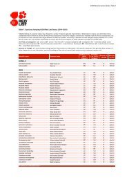
Table 2.1. Summary of the five criteria (A-E) used to evaluate if a taxon belongs in a threatened category
(Critically Endangered, Endangered or Vulnerable).
Use any of the criteria A–E Critically Endangered Endangered Vulnerable
A. Population reduction Declines measured over the longer of 10 years or 3 generations
A1 ≥ 90% ≥ 70% ≥ 50%
A2, A3 & A4 ≥ 80% ≥ 50% ≥ 30%
A1. Population reduction observed, estimated, inferred, or suspected in the past where the causes of the reduction are clearly
reversible AND understood AND have ceased, based on and specifying any of the following:
(a) direct observation
(b) an index of abundance appropriate to the taxon
(c) a decline in area of occupancy (AOO), extent of occurrence (EOO) and/or habitat quality
(d) actual or potential levels of exploitation
(e) effects of introduced taxa, hybridization, pathogens, pollutants, competitors or parasites.
A2. Population reduction observed, estimated, inferred, or suspected in the past where the causes of reduction may not have
ceased OR may not be understood OR may not be reversible, based on (a) to (e) under A1.
A3. Population reduction projected or suspected to be met in the future (up to a maximum of 100 years) based on (b) to (e)
under A1.
A4. An observed, estimated, inferred, projected or suspected population reduction (up to a maximum of 100 years) where the
time period must include both the past and the future, and where the causes of reduction may not have ceased OR may not
be understood OR may not be reversible, based on (a) to (e) under A1.
B. Geographic range in the form of either B1 (extent of occurrence) AND/OR B2 (area of occupancy)
B1. Extent of occurrence (EOO) < 100 km² < 5,000 km² < 20,000 km²
B2. Area of occupancy (AOO) < 10 km² < 500 km² < 2,000 km²
AND at least 2 of the following:
(a) Severely fragmented, OR
Number of locations = 1 ≤ 5 ≤ 10
(b) Continuing decline in any of: (i) extent of occurrence; (ii) area of occupancy; (iii) area, extent and/or quality of habitat;
(iv) number of locations or subpopulations; (v) number of mature individuals.
(c) Extreme fluctuations in any of: (i) extent of occurrence; (ii) area of occupancy; (iii) number of locations or
subpopulations; (iv) number of mature individuals.
C. Small population size and decline
Number of mature individuals < 250 < 2,500 < 10,000
AND either C1 or C2:
C1. An estimated continuing
decline of at least:
25% in 3 years or 1 20% in 5 years or 2
generation
generations
(up to a max. of 100 years in future)
C2. A continuing decline AND (a) and/or (b):
(a i) Number of mature individuals
in each subpopulation:
or
< 50 < 250 < 1,000
10% in 10 years or 3
generations
(a ii) % individuals
subpopulation =
in one
90–100% 95–100% 100%
(b) Extreme fluctuations in the number of mature individuals.
D. Very small or restricted population
Either:
Number of mature individuals < 50 < 250 D1. < 1,000
VU D2. Restricted area of occupancy or number of locations with a plausible
future threat that could drive the taxon to CR or EX in a very short time.
E. Quantitative Analysis
Indicating the probability of
extinction in the wild to be:
≥ 50% in 10 years or 3
generations (100 years max.)
≥ 20% in 20 years or 5
generations (100 years max.)
AND/OR
D2. typically: AOO

2.4 Conservation priorities and actions
The category of threat is not necessarily sufficient to determine priorities for conservation
action. The category of threat simply provides an assessment of the extinction risk under
current circumstances, whereas a system for assessing priorities for action will include
numerous other factors concerning conservation action such as costs, logistics, chances of
success, and other biological characteristics (Mace and Lande 1991). The Red List should
therefore not be interpreted as a means of priority setting (IUCN 2001). The difference
between measuring threats and assessing conservation priorities needs to be appreciated.
However, assessment of taxa using Red List Criteria represents a critical first step in setting
priorities for conservation action.
Many taxa assessed under the IUCN Red List Criteria will already be subject to some level
of conservation action. The criteria for the threatened categories are to be applied to a taxon
whatever the level of conservation action affecting it, and any conservation measures must be
included with the assessment documentation. It is important to emphasize here that a taxon
may require conservation action even if it is not listed as threatened, and that effectively
conserved threatened taxa may, as their status improves over time, cease to qualify for
listing.
2.5 Documentation
All assessments should be documented. Threatened classifications should state the criteria
and subcriteria that are met. For example, in a taxon listed as Endangered A2cd, the
criterion A2 indicates that the taxon has declined by more than 50% in the last 10 years or
three generations (whichever is longer) and the subcriteria indicate that the decline in mature
individuals has been caused by a decline in the quality of habitat as well as actual levels of
exploitation. Clearly listing the subcriteria provides the reasoning for placing a taxon in a
specific category, and if necessary, the reasoning can be re-examined. It also enables people
to understand the primary threats facing a taxon and may aid in conservation planning. No
assessment can be accepted for the IUCN Red List as valid unless at least one criterion and
any qualifying subcriteria are given. If more than one criterion or subcriterion is met, then
each should be listed. If a re-evaluation indicates that the documented criterion is no longer
met, this should not result in automatic reassignment to a lower category of threat
(downlisting). Instead, the taxon should be re-evaluated against all the criteria to clarify its
status. The factors responsible for qualifying the taxon against the criteria, especially where
inference and projection are used, should be documented. All data used in a listing must be
either referenced to a publication that is available in the public domain, or else be made
available. Full documentation requirements are given in Annex 3 of the IUCN Red List
Categories and Criteria (Version 3.1) (IUCN 2001).
3. Data Quality
3.1 Data availability, inference and projection
The IUCN Red List Criteria are intended to be applied to taxa at a global scale. However, it
is very rare for detailed and relevant data to be available across the entire range of a taxon.
For this reason, the Red List Criteria are designed to incorporate the use of inference and
projection, to allow taxa to be assessed in the absence of complete data. Although the
criteria are quantitative in nature, the absence of high-quality data should not deter attempts

Red List Guidelines 16
at applying the criteria. In addition to the quality and completeness of the data (or lack of),
there may be uncertainty in the data itself, which needs to be considered in a Red List
assessment. Data uncertainty is discussed separately in section 3.2.
The IUCN criteria use the terms Observed, Estimated, Projected, Inferred, and Suspected to
refer to the quality of the information for specific criteria. For example, criterion A allows
inferred or suspected reduction, whereas criterion C1 allows only estimated declines and
criterion C2 specifies “observed, projected, or inferred” declines. These terms are defined as
follows:
Observed: information that is directly based on well-documented observations of all known
individuals in the population.
Estimated: information that is based on calculations that may include statistical assumptions
about sampling, or biological assumptions about the relationship between an observed
variable (e.g., an index of abundance) to the variable of interest (e.g., number of mature
individuals). These assumptions should be stated and justified in the documentation.
Estimation may also involve interpolation in time to calculate the variable of interest for
a particular time step (e.g., a 10-year reduction based on observations or estimations of
population size 5 and 15 years ago). For examples, see discussion under criterion A.
Projected: same as “estimated”, but the variable of interest is extrapolated in time towards
the future. Projected variables require a discussion of the method of extrapolation (e.g.,
justification of the statistical assumptions or the population model used) as well as the
extrapolation of current or potential threats into the future, including their rates of
change.
Inferred: information that is based on indirect evidence, on variables that are indirectly
related to the variable of interest, but in the same general type of units (e.g., number of
individuals or area or number of subpopulations). Examples include population
reduction (A1d) inferred from a change in catch statistics, continuing decline in number
of mature individuals (C2) inferred from trade estimates, or continuing decline in area of
occupancy (B1b(ii,iii), B2b(ii,iii)) inferred from rate of habitat loss. Inferred values rely
on more assumptions than estimated values. For example, inferring reduction from
catch statistics not only requires statistical assumptions (e.g., random sampling) and
biological assumptions (about the relationship of the harvested section of the population
to the total population), but also assumptions about trends in effort, efficiency, and
spatial and temporal distribution of the harvest in relation to the population. Inference
may also involve extrapolating an observed or estimated quantity from known
subpopulations to calculate the same quantity for other subpopulations. Whether there
are enough data to make such an inference will depend on how large the known
subpopulations are as a proportion of the whole population, and the applicability of the
threats and trends observed in the known subpopulations to the rest of the taxon. The
method of extrapolating to unknown subpopulations depends on the criteria and on the
type of data available for the known subpopulations. Further guidelines are given under
specific criteria (e.g., see section 5.8 for extrapolating population reduction for criterion
A assessments).

Red List Guidelines 17
Suspected: information that is based on circumstantial evidence, or on variables in different
types of units, for example, % population reduction based on decline in habitat quality
(A1c) or on incidence of a disease (A1e). For example, evidence of qualitative habitat
loss can be used to infer that there is a qualitative (continuing) decline, whereas
evidence of the amount of habitat loss can be used to suspect a population reduction at a
particular rate. In general, a suspected population reduction can be based on any factor
related to population abundance or distribution, including the effects of (or dependence
on) other taxa, so long as the relevance of these factors can be reasonably supported.
3.2 Uncertainty
The data used to evaluate taxa against the criteria are often obtained with considerable
uncertainty. Uncertainty in the data should not be confused with a lack of data for certain
parts of a species’ range or a lack of data for certain parameters. This problem is dealt with
in section 3.1 (Data availability, inference and projection). Data uncertainty can arise from
any one or all of the following three factors: natural variability, vagueness in the terms and
definitions used in the criteria (semantic uncertainty), and measurement error (Akçakaya et
al. 2000). The way in which uncertainty is handled can have a major influence on the results
of an evaluation. Details of methods recommended for handling uncertainty are given
below.
3.2.1 Types of uncertainty
Natural variability results from the fact that species’ life histories and the environments in
which they live change over time and space. The effect of this variation on the criteria is
limited, because each parameter refers to a specific time or spatial scale. However, natural
variability can be problematic, e.g. there is spatial variation in age-at-maturity for marine
turtles, and a single estimate for these taxa needs to be calculated to best represent the
naturally occurring range of values. Semantic uncertainty arises from vagueness in the
definition of terms in the criteria or lack of consistency in different assessors’ usage of them.
Despite attempts to make the definitions of the terms used in the criteria exact, in some cases
this is not possible without the loss of generality. Measurement error is often the largest
source of uncertainty; it arises from the lack of precise information about the quantities used
in the criteria. This may be due to inaccuracies in estimating values or a lack of knowledge.
Measurement error may be reduced or eliminated by acquiring additional data (Akçakaya et
al. 2000; Burgman et al. 1999). Another source of measurement error is ‘estimation error’,
i.e. sampling the wrong data or the consequences of estimating a quantity (e.g., natural
mortality) based on a weak estimation method. This source of measurement error is not
necessarily reduced by acquiring additional data.
3.2.2 Representing uncertainty
Uncertainty may be represented by specifying a best estimate and a range of plausible values
for a particular quantity. The best estimate can itself be a range, but in any case the best
estimate should always be included in the range of plausible values. The plausible range
may be established using various methods, for example based on confidence intervals, the
opinion of a single expert, or the consensus view of a group of experts. The method used
should be stated and justified in the assessment documentation.

Red List Guidelines 18
3.2.3 Dispute tolerance and risk tolerance
When interpreting and using uncertain data, attitudes toward risk and uncertainty are
important. First, assessors need to consider whether they will include the full range of
plausible values in assessments, or whether they will exclude extreme values from
consideration (known as dispute tolerance). Uncertainty in the data is reduced when an
assessor has a high dispute tolerance, and thus excludes extreme values from the assessment.
We suggest assessors adopt a moderate attitude, taking care to identify the most likely
plausible range of values, excluding extreme or unlikely values.
Second, assessors need to consider whether they have a precautionary or evidentiary attitude
to risk (known as risk tolerance). A precautionary attitude (i.e., low risk tolerance) will
classify a taxon as threatened unless it is highly unlikely that it is not threatened, whereas an
evidentiary attitude will classify a taxon as threatened only when there is strong evidence to
support a threatened classification.
3.2.4 Dealing with uncertainty
It is recommended that assessors should adopt a precautionary but realistic attitude, and to
resist an evidentiary attitude to uncertainty when applying the criteria (i.e., have low risk
tolerance). This may be achieved by using plausible lower bounds, rather than best
estimates, in determining the quantities used in the criteria. It is recommended that ‘worst
case scenario’ reasoning be avoided as this may lead to unrealistically precautionary listings.
All attitudes should be explicitly documented. In situations where the spread of plausible
values (after excluding extreme or unlikely values) qualifies a taxon for two or more
categories of threat, the precautionary approach would recommend that the taxon be listed
under the higher (more threatened) category.
In some rare cases, uncertainties may result in two non-consecutive plausible threat
categories. This may happen, for example, when extent of occurrence (EOO) or area of
occupancy (AOO) is smaller than the EN threshold and one subcriterion is definitively met,
but it is uncertain whether a second subcriterion is also met. Depending on this, the category
can be either EN or NT. In such cases, the category could be specified as the range EN–NT
in the documentation (giving the reasons why), and the assessors must choose the most
plausible of the categories, of which VU could be one. This choice depends on the level of
precaution (see section 3.2.3) and should be justified.
Specific guidelines for dealing with uncertainty in assessing taxa with widely distributed or
multiple subpopulations against criterion A are given in section 5.8. This section offers clear
guidance on using uncertain estimates, uncertainty about the pattern of population decline
and using data with different abundance units.
3.2.5 Documenting uncertainty and interpreting listings
The level of uncertainty associated with a particular taxon’s assessment is not apparent from
the listing itself, potentially complicating and de-valuing interpretation of listings. When a
plausible range for each quantity is used to evaluate the criteria, a range of categories may be

Red List Guidelines 19
obtained, reflecting the uncertainties in the data. However, only a single category, based on a
specific attitude to uncertainty, will be listed along with the relevant criteria on the IUCN
Red List. It is important to note that the range of possible categories should also be
indicated, along with the assessors’ attitudes to uncertainty, in the documentation
accompanying the assessment. The inclusion of information on uncertainty in the
documentation, allows users of the Red List access to important information that will assist
in the interpretation of listings, and inform debates over particular issues or listings.
3.2.6 Uncertainty and the application of the categories Data Deficient and Near
Threatened
The level of uncertainty in the data used for assessments may or may not affect the
application of the categories Data Deficient and Near Threatened. Guidance on the
application of these categories is given in section 10.
4. Guidelines for the Definitions of Terms Used in the Criteria
The terms used in the IUCN Red List Categories and Criteria must be clearly understood to
ensure that taxa are correctly assessed. The following terms are defined in the IUCN Red
List Categories and Criteria (version 3.1) on pages 10-13 (IUCN 2001). These definitions
are reproduced here, with additional guidelines to assist in their interpretation.
4.1 Population and population size (criteria A, C and D)
“The term ‘population’ is used in a specific sense in the Red List Criteria that is different to
its common biological usage. Population is here defined as the total number of individuals
of the taxon. For functional reasons, primarily owing to differences between life forms,
population size is measured as numbers of mature individuals only. In the case of taxa
obligately dependent on other taxa for all or part of their life cycles, biologically appropriate
values for the host taxon should be used.” (IUCN 2001)
The interpretation of this definition depends critically on an understanding of the definition
of ‘mature individuals’, which is given and discussed below in section 4.3.
4.2 Subpopulations (criteria B and C)
“Subpopulations are defined as geographically or otherwise distinct groups in the population
between which there is little demographic or genetic exchange (typically one successful
migrant individual or gamete per year or less).” (IUCN 2001)
The significance of subpopulations in the criteria relates to the additional risks faced by taxa
where the population is either fragmented into many small units or where most individuals
are concentrated into one unit. Operational methods for determining the number of
subpopulations may vary according to the taxon; in the case of tree species, for example, a
subpopulation can be defined as a spatially distinct segment of the population that
experiences insignificant seed or pollen migration from other subpopulations within a
generation.

Red List Guidelines 20
Although subpopulations typically have little demographic or genetic exchange, this may or
may not amount to their complete isolation in this regard.
4.3 Mature individuals (criteria A, B, C and D)
“The number of mature individuals is the number of individuals known, estimated or
inferred to be capable of reproduction. When estimating this quantity the following points
should be borne in mind:
• Mature individuals that will never produce new recruits should not be counted (e.g.,
densities are too low for fertilization).
• In the case of populations with biased adult or breeding sex ratios, it is appropriate to use
lower estimates for the number of mature individuals, which take this into account.
• Where the population size fluctuates, use a lower estimate. In most cases this will be
much less than the mean.
• Reproducing units within a clone should be counted as individuals, except where such
units are unable to survive alone (e.g., corals).
• In the case of taxa that naturally lose all or a subset of mature breeding individuals at
some point in their life cycle, the estimate should be made at the appropriate time, when
mature individuals are available for breeding.
• Re-introduced individuals must have produced viable offspring before they are counted as
mature individuals.” (IUCN 2001)
4.3.1 Notes on defining mature individuals
This definition of mature individuals differs slightly from that given in version 2.3 of the Red
List Categories and Criteria (IUCN 1994). Some groups have found the more recent
definition of mature individuals to be less conservative and less precise, leading to a
potential down-listing of some taxa (e.g., obligate co-operative breeders) even though their
extinction risk has not changed. It must be stressed that the intention of the definition of
mature individuals is to allow the estimate of the number of mature individuals to take
account of all the factors that may make a taxon more vulnerable than might otherwise be
expected. The list of points given with the definition is not exhaustive and should not
restrict an assessor’s interpretation of mature individuals, provided they are estimating the
number of individuals known, estimated or inferred to be capable of reproduction. The
ability of an assessor to estimate or infer which individuals are capable of reproduction is
paramount and highly contingent on the particular features of the taxon or group. Juveniles,
senescent individuals, suppressed individuals and individuals in subpopulations whose
densities are too low for fertilization to occur will never produce new recruits, and therefore
should not be counted as mature individuals. On the other hand, in many taxa there is a pool
of non-reproductive (e.g., suppressed) individuals that will quickly become reproductive if a
mature individual dies. These individuals can be considered to be capable of reproduction.
In general, the judgement will be best made by assessors with insight into the species’
biology.
In the case of taxa obligately dependent on other taxa for all or part of their life cycles,
biologically appropriate values of mature individuals for the host taxon might be used. This

Red List Guidelines 21
number may be much less than the total number of mature individuals of the host taxon,
because generally other factors restrict the dependant taxon from utilizing all host
individuals.
The number of mature individuals can be estimated using the equation d * A * p, where d is
an estimate of population density, A is an estimate of area, and p is an estimate of the
proportion of individuals that are mature. However, this approach often leads to gross
overestimates of number of mature individuals. Therefore, great care should be taken when
using this formula to ensure that: (a) the area is appropriately selected and d is an estimate of
the average over the entire A (for example, the estimate will be positively biased if A is set to
EOO and d is based on samples from areas of highest density), and (b) p should be selected
based on knowledge of the taxon (or related taxa) rather than being set to a default value
(such as 0.5) because the proportion of mature individuals in a population differs markedly
among taxa. Bounds on the estimate of number of mature individuals can be obtained by
placing bounds on each of d, A, and p. The value from this approach will be an estimate if
the values for d, A and p are all estimates, but should be considered to be an inference if one
or more of these values are based on inference.
4.3.2 Colonial or modular organisms, such as corals, algae, bryophytes, fungi and many
vascular plants
As opposed to a unitary organism, such as a vertebrate, an insect and many vascular plants,
the growth and development of a colonial (modular) organism is an iterative process in
which “modules” are added step by step to the existing structure. In principle, the growth of a
modular organism never ends and it has no final shape, size or age. A modular organism (the
genet) can sometimes exist in a form of many parts (ramets), which can become more or less
isolated from each other. Consequently, what constitutes a ‘mature individual’ in a colonial
or modular organism is not always clear. Still, it is important to define ‘mature individual’
for such organisms, since ‘mature individual’ is used under criteria C and D to capture the
effects of threats and demographic stochasticity to a small population. In defining ‘mature
individual’ for colonial organisms, it is important to identify entities that are comparable in
extinction proneness to discrete mature individuals of animals and other organisms.
As a general rule, the ramet, i.e., the smallest entity capable of both independent survival and
(sexual or asexual) reproduction should be considered a ‘mature individual’. For instance, in
those cases where the organism appears in well-distinguishable units, each such unit would
be counted as one mature individual. Examples may be a bryophyte tuft (e.g., of Ulota) or a
discrete cushion (e.g., Brachythecium), a lichen thallus (e.g., Alectoria) or foliose patch (e.g.,
Parmelia), or a coral discrete entity (e.g., a brain coral Diploria or sun coral Tubastrea).
If the delimitation of ramets is not obvious, but the species lives in or on a discrete and
relatively small substrate unit limited by a certain resource, e.g. a piece of cow dung, a leaf or
a dead tree branch, each unit colonized by the species should be counted as a single mature
individual. In many other cases, like reef-forming corals, cliff-growing lichens and groundgrowing
fungi, the organism grows in large, more or less continuous entities that could be
divided into smaller pieces without obviously harming the organism. In principle, the
smallest such entity (ramet) that an organism could be divided into without causing its death

Red List Guidelines 22
or preventing reproduction, should be counted as one mature individual. Obviously, what
such an entity would be is often not known. Therefore, in such cases, it may be necessary to
adopt a pragmatic approach to defining ‘mature individuals’. Examples of possible
interpretations of the definition of a mature individual are:
• For diffuse, wholly visible organisms in continuous habitats (e.g., corals, algal mats)
assessors may assume an average area occupied by a mature individual and estimate the
number of mature individuals from the area of occupied habitat. The area of occupied
habitat should be estimated at a scale (grid size) that is as close as practicable to the area
assumed to be occupied by a single mature individual (not necessarily 2x2 km as
recommended for estimation of AOO).
• For diffuse organisms, not wholly visible, in continuous habitats (e.g., subterranean
mycelial fungi) assessors may assume that each recorded presence separated by a
minimum distance represents an assumed number of individuals. For example, each
visible fungal fruiting body may be assumed to represent ten mature individuals, so long
as they are separated by at least 10 metres. This kind of assumption is necessary because
the size or area of a fungal mycelium is rarely known.
• For diffuse organisms that occur in discrete habitat patches (e.g., fungi living more or
less concealed in dead wood), each patch (trunk or log colonized by the species) could –
if no better information exists – be counted as 2–10 mature individuals, depending on
the size of the tree.
In any case, it is recommended that authors of Red List assessments specify the way they
have used ‘mature individual’.
4.3.3 Fishes
In many taxa of marine fish, reproductive potential is commonly closely related to body size.
Since exploitation usually reduces the mean age and size of individuals, assessing declines in
numbers of mature individuals may under-estimate the severity of the decline. When
evaluating population decline, this factor should be kept in mind. One possible method is to
estimate decline in the biomass of mature individuals rather than the number of such
individuals when applying criterion A, where biomass is ‘an index of abundance appropriate
to the taxon’.
4.3.4 Sex-changing organisms
Many marine taxa have the capacity to change sex as they grow. In such taxa, the sex ratio
may be highly biased towards the smaller sex. The criteria acknowledge that the number of
mature individuals can take biased sex ratios into account, by using a lower estimate for the
number of mature individuals. For sex-changing organisms it is also appropriate to consider
changes in sex ratio as an indicator of population perturbation, which may be of additional
conservation concern because the larger sex (already less numerous) is often subject to
higher harvest mortality. In these cases, the number of mature individuals may be estimated
by doubling the average number of individuals of the larger (or less numerous) sex.

Red List Guidelines 23
4.3.5 Trees
Individual trees that flower without producing viable seeds do not qualify as mature
individuals. For example, Bailonella toxisperma first flowers at 50-70 years and does not
fruit until roughly 20 years later. Conversely, Sequoiadendron giganteum may produce seed
at less than 20 years of age and continue to do so for 3,000 years. However, not all trees
between these ages may be mature individuals if the population includes some reproductively
suppressed individuals. If little is known about age at fruiting, mature individuals should be
counted as those of a typical reproductive size; e.g. estimates for canopy taxa should exclude
sub-canopy individuals. Vegetative clones, apomictic taxa and self-fertilizing taxa may
qualify as mature individuals, so long as they produce viable offspring and their survival is
independent of other clones.
Where it is impossible to calculate the number of mature individuals, but information is
available on the total population size, it may be possible to infer the number of mature
individuals from the total population size.
4.4 Generation (criteria A, C1 and E)
“Generation length is the average age of parents of the current cohort (i.e., newborn
individuals in the population). Generation length therefore reflects the turnover rate of
breeding individuals in a population. Generation length is greater than the age at first
breeding and less than the age of the oldest breeding individual, except in taxa that breed
only once. Where generation length varies under threat, such as the exploitation of fishes,
the more natural, i.e. pre-disturbance, generation length should be used.” (IUCN 2001)
In general, time-based measures in the criteria are scaled for the different rates at which taxa
survive and reproduce, and generation length is used to provide this scaling. The current
definition of generation length has been widely misunderstood, and there are difficulties
when dealing with very long-lived taxa, with taxa having age-related variation in fecundity
and mortality, with variation in generation length under harvesting, with environmental
changes and variation between the sexes. Some of the different acceptable methods for
estimating generation length are included here.
It is also appropriate to extrapolate information such as a generation length from closely
related well-known taxa and to apply it to lesser-known and potentially threatened taxa.
Formally, there are several definitions of generation length, including the one given above;
mean age at which a cohort of newborns produce offspring; age at which 50% total
reproductive output is achieved; mean age of parents in a population at the stable age
distribution; and time required for the population to increase by the replacement rate. All of
these definitions of generation length require age- and sex-specific information on survival
and fecundity, and are best calculated from a life table (e.g., option 1 below). Depending on
the taxon concerned, other methods may provide a good approximation (e.g., options 2 and
3). Care should be taken to avoid estimates that may bias the generation length estimate in a
non-precautionary way, usually by under-estimating it. Generation length may be estimated
in a number of ways:

Red List Guidelines 24
1. the average age of parents in the population, based on the equation
G
∑
∑
= xlx
mx
l xm
x
where the summations are from age (x) 0 to the last age of reproduction; mx is
(proportional to) the fecundity at age x; and lx is survivorship up to age x
(i.e., lx = S0 · S1 ··· Sx-1 where S is annual survival rate, and l0 =1 by definition)
This formula is implemented in an associated spreadsheet file (Generation
length.xls). To use this formula, follow the instructions in the file, noting the exact
definitions of the parameters required.
2. 1/adult mortality + age of first reproduction. This approximation is useful if annual
mortality after the age of first reproduction is well known, and if mortality and
fecundity do not change with age after the age of first reproduction (i.e., there is no
senescence). Many species exhibit senescence, with mortality increasing and
fecundity decreasing with age; for these species, this formula will overestimate
generation length (in such cases, use the spreadsheet mentioned above). For age of
first reproduction, use the age at which individuals first produce offspring in the wild
(which may be later than when they are biologically capable of breeding), averaged
over all individuals or all females. If first reproduction typically occurs by 12
months, use 0, not 1; if it occurs between 12 and 24 months, use 1, etc.
3. age of first reproduction + z * (length of the reproductive period), where z is usually

Red List Guidelines 25
It is not necessary to calculate an average or typical generation length if some subpopulations
of the taxon differ in terms of generation length. Instead, use each subpopulation's
generation length to calculate the reduction over the appropriate number of generations, and
then calculate the overall population reduction (for criterion A) or overall estimated
continuing decline (for criterion C1) using a weighted average of the reductions calculated
for each subpopulation, where the weight is the size of the subpopulation 3 generations ago
(see detailed explanation and examples in section 5.8).
4.5 Reduction (criterion A)
“A reduction is a decline in the number of mature individuals of at least the amount (%)
stated under the criterion over the time period (years) specified, although the decline need
not be continuing. A reduction should not be interpreted as part of a fluctuation unless there
is good evidence for this. The downward phase of a fluctuation will not normally count as a
reduction.” (IUCN 2001)
4.5.1 Estimating reduction
Percentage reductions in the number of mature individuals can be estimated in a number of
ways, including ‘an index of abundance appropriate to the taxon’. In the case of exploited
fishes, the catch per unit effort (CPUE) may be used. This measure should be used with
caution because changes in CPUE may underestimate population declines. This may occur,
for example, if the population aggregates even at small sizes so that catches remain high with
the same level of effort, even if the size of the population is declining. It may also occur if
increases in fishing efficiency are not fully taken into account. It is therefore preferable to
assess exploited fish taxa using the results of fishery-independent survey techniques.
The population data from which a reduction can be calculated are likely to be variable, and it
may not be obvious how a reduction should best be estimated. Depending on the shape of
the data, a linear or exponential model may be fitted, and the start and end points of the fitted
line used to calculate the reduction. Fitting a model in this way helps to eliminate some of
the variability in the data that may be attributable to natural fluctuations, which should not be
included. If populations fluctuate widely, or oscillate with periods longer than generation
time, fitting a time series longer than three generations may give a more representative
estimate of the long-term population reduction. However, regardless of the length of the
time series fitted, the reduction should be calculated for the most recent three generations.
The model to be fitted should be based on the pattern of decline, which may be inferred from
the type of threat. If a taxon is threatened by exploitation, and the hunting mortality
(proportion of individuals taken) does not change as the population size declines, then the
population is likely to be declining exponentially, and this model should be fitted. In some
cases, a linear model will be more appropriate. This occurs when the number of individuals
taken (rather than their proportion to the total population) may remain constant. For
example, if a taxon is threatened with habitat loss, and a similar sized area of habitat is lost
every year, this could lead to a linear decline in the number of individuals. No model need be
fitted in cases where there are only two estimates of population size (at the start and end of
the time period specified in the criteria) – the reduction can be calculated from those two
points. If a model is fitted, the assumptions of the model must be justified by characteristics

Red List Guidelines 26
of life history, habitat biology, pattern of exploitation or other threatening processes, etc. For
more information, see section 5.8 below).
4.5.2 Inferring or projecting population reduction
When it is necessary to extrapolate population trends (under criteria A3 or A4), the assumed
pattern of decline (e.g., exponential or linear) can make an important difference to the
assessment. Guidelines on this issue are given in section 5 (criterion A).
Population reduction over long generation times may be estimated from data over shorter
time frames. However, assumptions about the rate of decline remaining constant, increasing
or decreasing, relative to the observed interval must be justified with reference to threatening
processes, life history or other relevant factors. Section 3 deals with incorporating
uncertainty and using inference and projection.
Future population reduction can be projected using population models, provided that: (i) the
model meets the requirements outlined in section 9 ("Guidelines for Applying Criterion E"),
(ii) the effects of future levels of threat are included in the population model, represented as
changes in model parameters, and (iii) the model outputs are not inconsistent with expected
changes in current or recent rates of decline. When using a population model to project a
reduction under criterion A3, the median or mean of the projections for a range of plausible
scenarios should be used to calculate a best estimate of the magnitude of the projected
reduction. Assessments may be based on the best estimate, lower or upper bound but, for
reasons of transparency, assessors must justify the rationale for their choice if a value other
than the best estimate is used. The projected variability may be used to quantify uncertainty.
For example, upper and lower quartiles of the projected magnitude of the future reduction
(i.e., reductions with 25% and 75% probability) may be considered to represent a plausible
range of projected reduction, and used to incorporate uncertainty in the assessment, as
described in sections 3.2 and 5.8.2 of the Guidelines. The bounds of the plausible range
should incorporate model uncertainty as well as measurement error; or a justification of the
model structure, and why it is the most appropriate in the face of model uncertainty, should
be provided.
4.6 Continuing decline (criteria B and C)
“A continuing decline is a recent, current or projected future decline (which may be smooth,
irregular or sporadic) which is liable to continue unless remedial measures are taken.
Fluctuations will not normally count as continuing declines, but an observed decline should
not be considered as a fluctuation unless there is evidence for this.” (IUCN 2001)
Continuing declines are used in two different ways in the criteria. Continuing declines at any
rate can be used to qualify taxa under criteria B or C2. This is because taxa under
consideration for criteria B and C are already characterized by restricted ranges or small
population size. Estimated continuing decline (under criterion C1) has quantitative
thresholds, and requires a quantitative estimate. The concept of continuing decline at any
rate is not applicable under criterion C1 (or under criterion A).

Red List Guidelines 27
Under criteria B1b, B2b, and C2, continuing declines can be observed, estimated, inferred or
projected. Although not explicitly mentioned in criteria B or C2, estimated continuing
declines are permissible. Under criterion C1, continuing declines can only be observed,
estimated or projected. A continuing decline under B or C can be projected, thus, it does not
have to have started yet. However, such projected declines must be justified and there must
be high degree of certainty that they will take place (i.e., merely 'plausible' future declines are
not allowed).
Rates of continuing decline over long generation times (in the same way as reductions) may
be estimated from data over shorter time frames. For example, evaluating a taxon under
criterion C1 for the Vulnerable category requires estimating a continuing decline for three
generations or 10 years, whichever is longer (up to a maximum of 100 years). When
extrapolating data from shorter time frames, assumptions about the rate of decline remaining
constant, increasing or decreasing, relative to the observed interval must be justified with
reference to threatening processes, life history or other relevant factors.
Note that a continuing decline is not possible without a population reduction (which,
however, may not be large enough to meet any thresholds under criterion A), but a reduction
is possible without a continuing decline: if a reduction has ‘ceased’ under criterion A, there
cannot be a continuing decline. However, continuing declines need not be continuous; they
can be sporadic, occurring at unpredictable intervals, but they must be likely to continue into
the future. Relatively rare events can be considered to contribute to a continuing decline if
they happened at least once within the last three generations or 10 years (whichever is
longer), and it is likely that they may happen again in the next three generations or 10 years
(whichever is longer), and the population is not expected to recover between the events.
A potentially confusing aspect of the criteria is that “estimated continuing decline” under C1
is conceptually very similar to “moving window reduction” under A4. The differences are (i)
A4 is always evaluated for three generations/10 years, whereas C1 is evaluated for one, two
or three generations, depending on the category, (ii) the thresholds are lower under C1 (e.g.,
for VU, 10% under C1 and 30% under A4), (iii) C1 also requires small population size, and
(iv) under C1, the decline must be observed or estimated, whereas under A4, the reduction
can be observed, estimated, inferred, projected or suspected.
If habitat is declining but abundance is not, this may be because (i) there is a delay in the
population's response to lower carrying capacity (K), perhaps because the population is
below K for other reasons (such as harvest), (ii) habitat is declining in areas not currently
occupied by the taxon, or (iii) habitat is not correctly identified. In the case of (i), the
population will eventually be impacted; in the case of (ii) the loss of recolonization options
may eventually impact the population. In both cases, B1b(iii) or B2b(iii) may be invoked
even if the population is not undergoing a continuing decline. Incorrect habitat identification
(case iii) often requires a more precise definition of "habitat." When determining continuing
decline in area, extent and/or quality of habitat (criteria B1b(iii) and B2b(iii)), assessors
should define "habitat" in the strict sense, i.e., as the area, characterized by its abiotic and
biotic properties, that is habitable by a particular species. In particular, they should avoid
using generic classifications such as "forest" that indicate a biotope, a vegetation type, or a
land cover type, rather than a species-specific identification of habitat.

Red List Guidelines 28
4.7 Extreme fluctuations (criteria B and C2)
“Extreme fluctuations can be said to occur in a number of taxa where population size or
distribution area varies widely, rapidly and frequently, typically with a variation greater than
one order of magnitude (i.e., a tenfold increase or decrease).” (IUCN 2001)
Extreme fluctuations are included in criteria B and C in recognition of the positive
relationship between extinction risk and variance in the rate of population growth (Burgman
et al. 1993). Populations that undergo extreme fluctuations are likely to have highly variable
growth rates, and are therefore likely to be exposed to higher extinction risks than
populations with lower levels of variability.
Population fluctuations may vary in magnitude and frequency (Figure 4.1). For the ‘extreme
fluctuations’ subcriterion to be invoked, populations would normally need to fluctuate by at
least 10-fold (i.e., an order of magnitude difference between population minima and
maxima). Fluctuations may occur over any time span, depending on their underlying causes.
Short-term fluctuations that occur over seasonal or annual cycles will generally be easier to
detect than those that occur over longer time spans, such as those driven by rare events or
climatic cycles such as El Niño. Fluctuations may occur regularly or sporadically (i.e., with
variable intervals between successive population minima or successive population maxima).
The effect of extreme fluctuations on the extinction risk will depend on both the degree of
isolation and the degree of synchrony of the fluctuations between subpopulations.
If there is regular or occasional dispersal (of even a small number of individuals, seeds,
spores, etc) between all (or nearly all) of the subpopulations, then the degree of fluctuations
should be measured over the entire population. In this case, the subcriterion would be met
only when the overall degree of fluctuation (in the total population size) is larger than one
order of magnitude. If the fluctuations of different subpopulations are independent and
asynchronous, they would cancel each other to some extent when fluctuations of the total
population size are considered.
If, on the other hand, the subpopulations are totally isolated, the degree of synchrony
between the populations is not as important and it is sufficient that a majority of
subpopulations each show extreme fluctuation to meet the subcriterion. In this case, if most
of the subpopulations show fluctuations of an order of magnitude, then the criterion would
be met (regardless of the degree of the fluctuations in total population size).
Between these two extremes, if dispersal is only between some of the subpopulations, then
the total population size over these connected subpopulations should be considered when
assessing fluctuations; each set of connected subpopulations should be considered separately.
Population fluctuations may be difficult to distinguish from directional population changes,
such as continuing declines, reductions or increases. Figure 4.1 shows examples where
fluctuations occur independent of, and in combination with, directional changes. A reduction

Red List Guidelines 29
should not be interpreted as part of a fluctuation unless there is good evidence for this.
Fluctuations must be inferred only where there is reasonable certainty that a population
change will be followed by a change in the reverse direction within a generation or two. In
contrast, directional changes will not necessarily be followed by a change in the reverse
direction.
There are two main ways that extreme fluctuations may be diagnosed: (i) by interpreting
population trajectories based on an index of abundance appropriate for the taxon; and (ii) by
using life history characteristics or habitat biology of the taxon.
i) Population trajectories must show a recurring pattern of increases and decreases
(Figure 4.1). Normally, several successive increases and decreases would need to be
observed to demonstrate the reversible nature of population changes, unless an
interpretation of the data was supported by an understanding of the underlying cause
of the fluctuation (see ii). Successive maxima or minima may be separated by
intervals of relatively stable population size.
ii) Some organisms have life histories prone to boom/bust dynamics. Examples include
fish that live in intermittent streams, granivorous small mammals of arid climates,
and plants that respond to stand-replacing disturbances. In these cases there is
dependence on a particular resource that fluctuates in availability, or a response to a
disturbance regime that involves predictable episodes of mortality and recruitment.
An understanding of such relationships for any given taxon may be gained from
studies of functionally similar taxa, and inference of extreme fluctuations need not
require direct observation of successive increases and decreases.
In all cases, assessors must be reasonably certain that fluctuations in the number of mature
individuals represent changes in the total population, rather than simply a flux of individuals
between different life stages. For example, in some freshwater invertebrates of intermittent
water bodies, the number of mature individuals increases after inundation which stimulates
emergence from larval stages. Mature individuals reproduce while conditions remain
suitable, but die out as the water body dries, leaving behind immature life stages (e.g., eggs)
until the next inundation occurs. Similarly, fires may stimulate mass recruitment from large
persistent seed banks when there were few mature individuals before the event. As in the
previous example, mature plants may die out during the interval between fires, leaving a
store of immature individuals (seeds) until they are stimulated to germinate by the next fire.
Such cases do not fall within the definition of extreme fluctuations unless the dormant life
stages are exhaustible by a single event or cannot persist without mature individuals. Plant
taxa that were killed by fire and had an exhaustible canopy-stored seed bank (serotinous
obligate seeders), for example, would therefore be prone to extreme fluctuations because the
decline in the number of mature individuals represents a decline in the total number.

Red List Guidelines 30
Index of abundance
100
10
1
100
10
1
100
10
1
100
10
1
100
10
1
Time
(a)
(c)
(e)
(g)
(i)
100
10
1
100
10
1
100
10
1
100
10
4.8 Severely fragmented (criterion B)
1
(b)
(f)
(h)
(d)
Figure 4.1. Fluctuations without
directional change in population
size (a-d), population reductions or
declines without fluctuations (e-f),
population reductions in
combination with fluctuations (g-i).
“The phrase ‘severely fragmented’ refers to the situation in which increased extinction risks
to the taxon results from the fact that most of its individuals are found in small and relatively
isolated subpopulations (in certain circumstances this may be inferred from habitat
information). These small subpopulations may go extinct, with a reduced probability of
recolonization.” (IUCN 2001)
Fragmentation must be assessed at a scale that is appropriate to biological isolation in the
taxon under consideration. In general, taxa with highly mobile adult life stages or with a
large production of small mobile diaspores are considered more widely dispersed, and hence
not so vulnerable to isolation through fragmentation of their habitats. Taxa that produce only
small numbers of diaspores (or none at all), or only large ones, are less efficient at long
distance dispersal and therefore more easily isolated. If natural habitats have been

Red List Guidelines 31
fragmented (e.g., old growth forests and rich fens), this can be used as direct evidence for
fragmentation for taxa with poor dispersal ability.
In cases where data are available on (i) the distribution of area of occupancy (i.e., detailed
maps of occupied habitat), (ii) some aspect of the dispersal ability of the taxon, (e.g., average
dispersal distance), and (iii) average population density in occupied habitat (e.g., information
on territory size, home range size, etc.), then the following criterion can be used to decide
whether there is severe fragmentation: A taxon can be considered to be severely fragmented
if most (>50%) of its total area of occupancy is in habitat patches that are (1) smaller than
would be required to support a viable population, and (2) separated from other habitat
patches by a large distance
For (1), the area for a viable population should be based on rudimentary estimates of
population density, and on the ecology of the taxon. For example, for many vertebrates,
patches that can support fewer than a hundred individuals may be considered too small to be
viable. For (2), the degree of isolation of patches should be based on dispersal distance of
the taxon. For example, patches that are isolated by distances several times greater than the
(long-term) average dispersal distance of the taxon may be considered isolated.
Note that the existence (or even a large number) of small and isolated patches is not
sufficient to consider the taxon severely fragmented. For meeting this criterion, more than
half of the individuals (or, more than half of the occupied habitat area) must be in small and
isolated patches.
For many taxa, the information on population density and dispersal distance can be based on
other similar taxa. Biologically informed values can be set by the assessors for large
taxonomic groups (families or even orders) or for other groupings of taxa based on their
biology. For example in bryophytes, information on the effects of isolation of
subpopulations is often lacking. It is recommended that in most circumstances, a minimum
distance greater than 50 km between subpopulations of taxa without spore dispersal can
indicate severe fragmentation, and a distance of between 100 km and 1,000 km for taxa with
spores (Hallingbäck et al. 2000).
The definition of severe fragmentation is based on the distribution of subpopulations. This is
often confused with the concept of "location" (see section 4.11), but is independent of it. A
taxon may be severely fragmented, yet all the isolated subpopulations may be threatened by
the same major factor (single location), or each subpopulation may be threatened by a
different factor (many locations).
4.9 Extent of occurrence (criteria A and B)
“Extent of occurrence is defined as the area contained within the shortest continuous
imaginary boundary which can be drawn to encompass all the known, inferred or projected
sites of present occurrence of a taxon, excluding cases of vagrancy. This measure may
exclude discontinuities or disjunctions within the overall distributions of taxa (e.g., large
areas of obviously unsuitable habitat) [but see 'area of occupancy', section 4.10 below].
Extent of occurrence can often be measured by a minimum convex polygon (the smallest

Red List Guidelines 32
polygon in which no internal angle exceeds 180 degrees and which contains all the sites of
occurrence).” (IUCN 2001)
Extent of occurrence (EOO) is a parameter that measures the spatial spread of the areas
currently occupied by the taxon. The intent behind this parameter is to measure the degree to
which risks from threatening factors are spread spatially across the taxon’s geographical
distribution. It is not intended to be an estimate of the amount of occupied or potential
habitat, or a general measure of the taxon’s range. Other, more restrictive definitions of
“range” may be more appropriate for other purposes, such as for planning conservation
actions. Valid use of the criteria requires that EOO is estimated in a way that is consistent
with the thresholds set therein.
In thinking about the differences between EOO and AOO (area of occupancy; discussed in
section 4.10), it may be helpful to compare species that have similar values for one of these
spatial parameters and different values for the other. All else being equal, larger EOOs
usually result in a higher degree of risk spreading (and hence a lower overall risk of
extinction to for the taxon) than smaller EOOs, depending on the relevant threats to the taxa.
For example, a taxon with occurrences distributed over a large area is highly unlikely to be
adversely affected across its entire range by a single fire because the spatial scale of a single
occurrence of this threat is narrower than the spatial distribution of the taxon. Conversely, a
narrowly distributed endemic taxon, with the same AOO as the taxon above, may be severely
affected by a fire across its entire EOO because the spatial scale of the threat is larger than, or
as large as, the EOO of the taxon.
In the case of migratory species, EOO should be based on the minimum of the breeding or
non-breeding (wintering) areas, but not both, because such species are dependent on both
areas, and the bulk of the population is found in only one of these areas at any time.
If EOO is less than AOO, EOO should be changed to make it equal to AOO to ensure
consistency with the definition of AOO as an area within EOO.
EOO can be measured by a minimum convex polygon and may exclude “discontinuities or
disjunctions within the overall distribution of the taxa”. However, for assessments of
criterion B, exclusion of areas forming discontinuities or disjunctions from estimates of EOO
is discouraged except in extreme circumstances. Exclusions are not recommended for
criterion B, because disjunctions and outlying occurrences accurately reflect the extent to
which a large range size reduces the chance that the entire population of the taxon will be
affected by a single threatening process. The risks are spread by the existence of outlying or
disjunct occurrences irrespective of whether the EOO encompasses significant areas of
unsuitable habitat. Inappropriate exclusions of discontinuities or disjunctions within the
overall distribution of a taxon will underestimate EOO for the purpose of assessing criterion
B and consequently will underestimate the degree to which risk is spread spatially for the
taxon. Further guidelines on the kind of discontinuities or disjunctions that should be
excluded will be developed following a review of current assessments.
When there are such discontinuities or disjunctions in a species distribution, the minimum
convex polygon (also called the convex hull) yields a boundary with a very coarse level of

Red List Guidelines 33
resolution on its outer surface, resulting in a substantial overestimate of the range,
particularly for irregularly shaped ranges (Ostro et al. 1999). The consequences of this bias
vary, depending on whether the estimate of EOO is to be used for assessing the spatial
thresholds in criterion B or whether it is to be used for estimating or inferring reductions
(criterion A) or continuing declines (criteria B and C). The use of convex hulls is unlikely to
bias the assessment of EOO thresholds under criterion B, because disjunctions and outlying
occurrences often do contribute to the spatial spread of risk (see above). However, the bias
associated with estimates based on convex hulls, and their sensitivity to sampling effort,
makes them less suitable as a method for comparing two or more temporal estimates of EOO
for assessing reductions or continuing declines. If outliers are detected at one time and not
another, this could result in erroneous inferences about reductions or increases. Therefore, a
method such as the α-hull (a generalization of a convex hull) is recommended for assessing
reductions of continuing declines in EOO because it substantially reduces the biases that may
result from the spatial arrangement of habitat (Burgman and Fox 2003). The α-hull provides
a more repeatable description of the external shape of a species’ range by breaking it into
several discrete patches when it spans uninhabited regions. For α-hulls the estimate of area
and trend in area also converges on the correct value as sample size increases, unless other
errors are large. This does not necessarily hold for convex hulls. Kernel estimators may be
used for the same purpose but their application is more complex.
To estimate an α-hull, the first step is to make a Delauney triangulation of the mapped points
of occurrence (Figure 4.2). The triangulation is created by drawing lines joining the points,
constrained so that no lines intersect between points. The outer surface of the Delauney
triangulation is identical to the convex hull.
Figure 4.2. Illustration of α-hull. The lines show the Delauney
triangulation (the intersection points of the lines are the taxon’s
occurrence locations). The sum of the areas of darker triangles is
EOO based on the α-hull. The two lighter coloured triangles that are
part of the convex hull are excluded from the α-hull.
The second step is to measure the lengths of all of the lines, and calculate the average line
length. The third step is to delete all lines that are longer than a multiple (α) of the average
line length. (This product of α and the average line length represents a “discontinuity

Red List Guidelines 34
distance”.) The value of α can be chosen with a required level of resolution in mind. The
smaller the value of α, the finer the resolution of the hull. Experience has shown that an α
value of 2 is a good starting point for some species (however, the value to use for specific
cases of assessing reductions in EOO should be based on a compromise between minimizing
the potential bias associated with incomplete sampling of outlying occurrences and
minimizing the departure from a convex hull). This process results in the deletion of lines
joining points that are relatively distant, and may subdivide the total range into more than
one polygon. The final step is to calculate the extent of occurrence by summing the areas of
all remaining triangles. When this exercise is repeated to estimate EOO from a second
temporal sample of points (and hence assess change in EOO), the same discontinuity
distance between points should be used as a threshold for deleting lines (rather than the same
value of α). This will reduce bias due to variation in sampling effort between the two surveys
and the bias due to changing average line length with more or fewer occurrences.
Extent of occurrence and area of occupancy are measures of the current distribution, i.e. they
should not include areas where the species no longer exists. On the other hand, these
measures should not only include the actually known sites, but also inferred sites. For
instance, sites can be inferred from presence of known appropriate habitat, but where the
species has not yet been searched for. In doing so, it will be important to judge to what extent
the taxon has been looked for. Incorporating inferred sites results in a range of plausible
values, which may give a range of plausible Red List Categories (see sections 3.1 on Data
availability, inference and projection, and 3.2 on Uncertainty).
4.10 Area of occupancy (criteria A, B and D)
“Area of occupancy is defined as the area within its 'extent of occurrence' (see 4.9 above),
which is occupied by a taxon, excluding cases of vagrancy. The measure reflects the fact
that a taxon will not usually occur throughout the area of its extent of occurrence, which may
contain unsuitable or unoccupied habitats. In some cases, (e.g., irreplaceable colonial
nesting sites, crucial feeding sites for migratory taxa) the area of occupancy is the smallest
area essential at any stage to the survival of existing populations of a taxon. The size of the
area of occupancy will be a function of the scale at which it is measured, and should be at a
scale appropriate to relevant biological aspects of the taxon, the nature of threats and the
available data (see below). To avoid inconsistencies and bias in assessments caused by
estimating area of occupancy at different scales, it may be necessary to standardize estimates
by applying a scale-correction factor. It is difficult to give strict guidance on how
standardization should be done because different types of taxa have different scale-area
relationships.” (IUCN 2001)
Area of occupancy (AOO) is a parameter that represents the area of suitable habitat currently
occupied by the taxon. As any area measure, AOO requires a particular scale. In this case,
the scale is determined by the thresholds in the criteria, i.e. valid use of the criteria requires
that AOO is estimated at scales that relate to the thresholds in the criteria. These scales (see
“Problems of scale” below) are intended to result in comparable threat status across taxa;
other scales may be more appropriate for other uses. For example, much finer scales are
appropriate for planning conservation action for plants, and larger scales may be appropriate

Red List Guidelines 35
for global gap analysis for large mobile species. However, such scales may not be
appropriate for use with the criteria.
Area of occupancy is included in the criteria for two main reasons. The first is to identify
species with restricted spatial distribution and, thus usually with restricted habitat. These
species are often habitat specialists. Species with a restricted habitat are considered to have
an increased risk of extinction. Secondly, in many cases, AOO can be a useful proxy for
population size, because there is generally a positive correlation between AOO and
population size. The veracity of this relationship for any one species depends on variation in
its population density.
Suppose two species have the same EOO, but different values for AOO, perhaps because one
has more specialized habitat requirements. For example, two species may be distributed
across the same desert (hence EOO is the same), but one is wide ranging throughout (large
AOO) while the other is restricted to oases (small AOO). The species with the smaller AOO
may have a higher risk of extinction because threats to its restricted habitat (e.g., degradation
of oases) are likely to reduce its habitat more rapidly to an area that cannot support a viable
population. The species with the smaller AOO is also likely to have a smaller population
size than the one with a larger AOO, and hence is likely to have higher extinction risks for
that reason.
4.10.1 Problems of scale
Classifications based on the area of occupancy (AOO) may be complicated by problems of
spatial scale. There is a logical conflict between having fixed range thresholds and the
necessity of measuring range at different scales for different taxa. “The finer the scale at
which the distributions or habitats of taxa are mapped, the smaller the area will be that they
are found to occupy, and the less likely it will be that range estimates … exceed the
thresholds specified in the criteria. Mapping at finer spatial scales reveals more areas in
which the taxon is unrecorded. Conversely, coarse-scale mapping reveals fewer unoccupied
areas, resulting in range estimates that are more likely to exceed the thresholds for the
threatened categories. The choice of scale at which AOO is estimated may thus, itself,
influence the outcome of Red List assessments and could be a source of inconsistency and
bias.” (IUCN 2001)
Some estimates of AOO may require standardization to an appropriate reference scale to
reduce such bias. Below, we first discuss a simple method of estimating AOO, then we
make recommendations about the appropriate reference scale, and finally we describe a
method of standardization for cases where the available data are not at the reference scale.
4.10.2 Methods for estimating AOO
There are several ways of estimating AOO, but for the purpose of these guidelines we
assume estimates have been obtained by counting the number of occupied cells in a uniform
grid that covers the entire range of a taxon (see Figure 2 in IUCN 2001), and then tallying the
total area of all occupied cells:
AOO = no. occupied cells × area of an individual cell (equation 4.1)

Red List Guidelines 36
The ‘scale’ of AOO estimates can then be represented by the area of an individual cell in the
grid (or alternatively the length of a cell, but here we use area). There are other ways of
representing AOO, for example, by mapping and calculating the area of polygons that
contain all occupied habitat. The scale of such estimates may be represented by the area of
the smallest mapped polygon (or the length of the shortest polygon segment), but these
alternatives are not recommended.
If different grid locations (starting points of the grid) result in different AOO estimates, the
minimum estimate should be used.
4.10.3 The appropriate scale
It is impossible to provide any strict but general rules for mapping taxa or habitats; the most
appropriate scale will depend on the taxon in question, and the origin and comprehensiveness
of the distribution data. However, we believe that in many cases a grid size of 2 km (a cell
area of 4 km 2 ) is an appropriate scale. Scales of 3.2 km grid size or coarser (larger) are
inappropriate because they do not allow any taxa to be listed as Critically Endangered (where
the threshold AOO under criterion B is 10 km 2 ). Scales of 1 km grid size or smaller tend to
list more taxa at higher threat categories than these categories imply. For most cases, we
recommend a scale of 4 km 2
cells as the reference scale. If an estimate was made at a
different scale, especially if data at different scales were used in assessing species in the
same taxonomic group, this may result in inconsistencies and bias. In any case, the scale for
AOO should not be based on EOO (or other measures of range area), because AOO and
EOO measure different factors affecting extinction risk (see above).
If AOO can be calculated at the reference scale of 4 km 2
cells, you can skip sections 4.10.4
and 4.10.5. If AOO cannot be calculated at the reference scale (e.g., because it has
already been calculated at another scale and original maps are not available), then the
methods described in the following two sections may be helpful.
4.10.4 Scale-area relationships
We recommended reducing the biases caused by use of range estimates made at different
scales by standardizing estimates to a reference scale that is appropriate to the thresholds in
the criteria. This and the following section discuss the scale-area relationship that forms the
background for these standardization methods, and describe such a method with examples.
The method of standardization depends on how AOO is estimated. In the following
discussion, we assume that AOO was estimated using the grid method summarized above.
The standardization or correction method we will discuss below relies on the relationship of
scale to area, in other words, how the estimated AOO changes as the scale or resolution
changes. Estimates of AOO may be calculated at different scales by starting with mapped
locations at the finest spatial resolution available, and successively doubling the dimensions
of grid cells. The relationship between the area occupied and the scale at which it was
estimated may be represented on a graph known as an area-area curve (e.g., Figure 4.3). The
slopes of these curves may vary between theoretical bounds, depending on the extent of grid
saturation. A maximum slope = 1 is achieved when there is only one occupied fine-scale grid

Red List Guidelines 37
cell in the landscape (fully unsaturated distribution). A minimum slope = 0 is achieved when
all fine-scale grid cells are occupied (fully saturated distribution).
grid
length
grid area AOO
1 1 10
2 4 24
4 16 48
8 64 64
16 256 256
32 1,024 1,024
Figure 4.3. Illustration of scale-dependence when calculating area of occupancy. At a fine
scale (map on right) AOO = 10 x 1 = 10 units 2 . At a coarse scale (map on left) AOO = 3 x
16 = 48 units 2
. AOO may be calculated at various scales by successively doubling grid
dimensions from estimates at the finest available scale (see Table). These may be
displayed on an area-area curve (above).
4.10.5 Scale correction factors
AOO
10000
1000
100
10
1
1 10 100 1000 10000
Scale (grid area)
Estimates of AOO may be standardized by applying a scale-correction factor. Scale-area
relationships (e.g., Figure. 4.3) provide important guidance for such standardization. It is not
possible to give a single scale-correction factor that is suitable for all cases because different
taxa have different scale-area relationships. Furthermore, a suitable correction factor needs to
take into account a reference scale (e.g., 2 km grid size) that is appropriate to the area of
occupancy thresholds in criterion B. The example below shows how estimates of AOO made
at fine and coarse scales may be scaled up and down, respectively, to the reference scale to
obtain an estimate that may be assessed against the AOO thresholds in criterion B.
Example: Scaling Up
Assume that estimates of AOO are available at 1 km grid resolution shown in Figure 4.3
(right) and that it is necessary to obtain an estimate at the reference scale represented by a
2 km grid. This may be done cartographically by simply doubling the original grid
dimensions, counting the number of occupied cells and applying equation 4.1. When the

Red List Guidelines 38
reference scale is not a geometric multiple of the scale of the original estimate, it is necessary
to calculate an area-area curve, as shown in Figure 4.3, and interpolate an estimate of AOO
at the reference scale. This can be done mathematically by calculating a scale correction
factor (C) from the slope of the area-area curve as follows (in all equations below, "log"
means logarithm to base 10):
C = log(AOO2/AOO1) / log(Ag2/Ag1)
(equation 4.2)
where AOO1
is the estimated area occupied from grids of area Ag1, a size close to, but
smaller than the reference scale, and AOO2 is the estimated area occupied from grids of area
Ag2, a size close to, but larger than the reference scale. An estimate of AOOR at the
reference scale, AgR,
may thus be calculated by rearranging equation 2 as follows:
AOOR
= AOO1*10 C*log(AgR / Ag1 ) , or AOOR = AOO2*10 C*log(AgR / Ag2 )
(equation
4.3)
In the example shown in Figure 4.3, estimates of AOO from 1x1 km and 4x4 km grids may
be used to verify the estimate AOO at the reference scale of 2x2 km as follows:
C = log(48/10) / log(16/1) = 0.566, and using equation 4.3 with this value of C, the
AOO estimate at the larger scale (AOO2=48), and the grid sizes at the larger and reference
scales (AgR=4; Ag2=16),
the AOO estimate at the reference scale is calculated as:
0.566*log(4/16) 2
AOO = 48 * 10 = 22 km
Note that this estimate differs slightly from the true value obtained from grid counting and
equation 1 (24 km 2
) because the slope of the area-area curve is not exactly constant between
the measurement scales of 1x1 km and 4x4 km.
Example: Scaling Down
Scaling down estimates of AOO is more difficult than scaling up because there is no
quantitative information about grid occupancy at scales finer than the reference scale. Scaling
therefore requires extrapolation, rather than interpolation of the area-area curve. Kunin
(1998) and He and Gaston (2000) suggest mathematical methods for this. A simple approach
is to apply equation 4.3 using an approximated value of C.
An approximation of C may be derived by calculating it at coarser scales, as suggested by
Kunin (1998). For example, to estimate AOO at 2x2 km when the finest resolution of
available data is at 4x4 km, we could calculate C from estimates at 4x4 km and 8x8 km as
follows.
C = log(64/48) / log(64/16) = 0.208
However, this approach assumes that the slope of the area-area curve is constant, which is
unlikely to hold for many taxa across a moderate range of scales. In this case, AOO at 2x2
km is overestimated because C was underestimated.
AOO = 48 * 10 0.208*log(4/16) = 36 km 2
.
While mathematical extrapolation may give some guidance in estimating C, there may be
qualitative information about the dispersal ability, habitat specificity and landscape patterns
that could also provide guidance. Table 4.1 gives some guidance on how these factors may

Red List Guidelines 39
influence the values of C within the range of scales between 2x2 km and 10x10 km grid
sizes.
Table 4.1. Characteristics of organisms and their habitat that influence the slope
of the scale-area relationship, and hence the scale-correction factor, C, within
the range of spatial scales represented by 2x2 km and 10x10 km grid cells.
Biological
Influence on C
characteristic small (approaching 0) large (approaching 1)
Dispersal ability Wide localized or sessile
Habitat specificity Broad Narrow
Habitat availability Extensive Limited
For example, if the organism under consideration was a wide-ranging animal without
specialized habitat requirements in an extensive and relatively uniform landscape (e.g., a
species of camel in desert), its distribution at fine scale would be relatively saturated and the
value of C would be close to zero. In contrast, organisms that are either sessile or wide
ranging but have specialized habitat requirements that only exist in small patches within the
landscape (e.g., migratory sea birds that only breed on certain types of cliffs on certain types
of islands) would have very unsaturated distributions represented by values of C close to one.
Qualitative biological knowledge about organisms and mathematical relationships derived
from coarse-scale data may thus both be useful for estimating a value of C that may be
applied in equation 4.3 to estimate AOO at the reference scale.
Finally, it is important to note that if unscaled estimates of AOO at scales larger than the
reference value are used directly to assess a taxon against thresholds in criterion B, then the
assessment is assuming that the distribution is fully saturated at the reference scale (i.e.,
assumes C = 0). In other words, the occupied coarse-scale grids are assumed to contain no
unsuitable or unoccupied habitat that could be detected in grids of the reference size (see
Figure 4.4).
4.10.6 "Linear" habitat
There is a concern that grids do not have much ecological meaning for taxa living in "linear"
habitat such as in rivers or along coastlines. Although this concern is valid, for the purpose
of assessing taxa against criterion B, it is important to have a measurement system that is
consistent with the thresholds, and that leads to comparable listings. If AOO estimates were
based on estimates of length x breadth of habitat, there may be very few taxa that exceed the
VU threshold for criterion B (especially when the habitats concerned are streams or beaches
a few metres wide). In addition, there is the problem of defining what a "linear" habitat is,
and measuring the length of a jagged line. Thus, we recommend that the methods described
above for estimating AOO should be used for taxa in all types of habitat distribution,
including taxa with linear ranges living in rivers or along coastlines.

Red List Guidelines 40
Observed 10km cell
Present
Absent
C = 0 C = 0.32 C = 0.5 C = 0.66 C = 1
Examples of assumed distributions within the same 100km 2 area, at the reference scale of
2x2km, with different C values
Figure 4.4. Demonstration of the consequences of different assumed C values. The
available map is at 10x10 km resolution, so a presence observed at this scale corresponds
to 25 cells at the reference scale of 2x2 km. Assuming C=0 (i.e., using the unscaled
estimate directly as AOO) assumes that all of these 25 cells are occupied. At the other
extreme, a value of C=1 assumes that only one 2x2 km cell is occupied.
4.10.7 AOO based on habitat maps and models
Habitat maps show the distribution of suitable habitat for a species. They may be derived
from interpretation of remote imagery and/or analyses of spatial environmental data using
simple combinations of GIS data layers, or by more formal statistical habitat models (e.g.,
generalized linear and additive models, decision trees, Bayesian models, regression trees,
etc.). Habitat maps can provide a basis for estimating AOO and EOO and, if maps are
available for different points in time, rates of change can be estimated. They cannot be used
directly to estimate a taxon’s AOO because they often map an area that is larger than the
occupied habitat (i.e., they also map areas of suitable habitat that may presently be
unoccupied). However, they may be a useful means of estimating AOO indirectly, provided
the three following conditions are met.
i) Maps must be justified as accurate representations of the habitat requirements of the
species and validated by a means that is independent of the data used to construct them.
ii) The mapped area of suitable habitat must be interpreted to produce an estimate of the
area of occupied habitat.
iii) The estimated area of occupied habitat derived from the map must be scaled to the grid
size that is appropriate for AOO of the species.
Habitat maps can vary widely in quality and accuracy (condition i). A map may not be an
accurate representation of habitat if key variables are omitted from the underlying model. For
example, a map would over-estimate the habitat of a forest-dependent montane species if it
identified all forest areas as suitable habitat, irrespective of altitude. The spatial resolution of
habitat resources also affects how well maps can represent suitable habitat. For example,
specialized nest sites for birds, such as a particular configuration of undergrowth or trees
with hollows of a particular size, do not lend themselves to mapping at coarse scales. Any
application of habitat maps to Red List assessment, should therefore be subject to an

Red List Guidelines 41
appraisal of mapping limitations, which should lead to an understanding of whether the maps
over-estimate or under-estimate the area of suitable habitat.
Habitat maps may accurately reflect the suitable habitat, but only a fraction of suitable
habitat may be occupied (condition ii). Low habitat occupancy may result because other
factors are limiting – such as availability of prey, impacts of predators, competitors or
disturbance, dispersal limitations, etc. In such cases, the area of mapped habitat could be
substantially larger than AOO and will therefore need to be adjusted (using an estimate of the
proportion of habitat occupied) to produce a valid estimate of AOO. This may be done by
random sampling of suitable habitat grid cells, which would require multiple iterations to
obtain a stable mean value of AOO. Habitat maps are produced at a resolution determined by
the input data layers (satellite images, digital elevation models, climate surfaces, etc.). Often
these will be at finer scales than those required to estimate AOO (condition iii), and
consequently scaling up will be required.
In those cases where AOO is less than the area of suitable habitat, the population may be
declining within the habitat, but the habitat may show no indication of change. Hence this
method could be both inaccurate and non-precautionary for estimating reductions in
population change.
However, if a decline in mapped habitat area is observed (and the map is a reasonable
representation of suitable habitat – condition i), then the population is likely to be declining
at least at that rate. This is a robust generalisation because even the loss of unoccupied
habitat can reduce population viability. Thus, if estimates of AOO are not available, then the
observed decline in mapped habitat area can be used to invoke "continuing decline" in
criteria B and C, and the rate of such decline can be used as a basis for calculating a lower
bound for population reduction under criterion A.
4.11 Location (criteria B and D)
“The term ‘location’ defines a geographically or ecologically distinct area in which a single
threatening event can rapidly affect all individuals of the taxon present. The size of the
location depends on the area covered by the threatening event and may include part of one or
many subpopulations. Where a taxon is affected by more than one threatening event,
location should be defined by considering the most serious plausible threat.” (IUCN 2001)
Justification for the number of locations used in Red List assessments should include
reference to the most serious plausible threat(s). For example, where the most serious
plausible threat is habitat loss, a location is an area where a single development project can
eliminate or severely reduce the population. Where the most serious plausible threat is
volcanic eruption, hurricane, tsunami, frequent flood or fire, locations may be defined by the
previous or predicted extent of lava flows, storm paths, inundation, fire paths, etc. Where
the most serious plausible threat is collection or harvest, then locations may be defined based
on the size of jurisdictions (within which similar regulations apply) or on the level of access
(e.g., ease with which collectors may reach different areas), as well as on the factors that
determine how the levels of exploitation change (e.g., if collection intensity in two separate
areas changes in response to the same market trends in demand, these may be counted as a
single location).

Red List Guidelines 42
If two or more subpopulations occur within an area that may be threatened by one such
event, they must be counted as a single location. Conversely, if a single subpopulation
covers an area larger than may be affected by any single event, it must be counted as more
than one location.
Where the most serious plausible threat does not affect all of the taxon’s distribution, other
threats can be used to define and count locations in those areas not affected by the most
serious plausible threat.
When parts of the distribution are not affected by any threat, the following options will be
appropriate under different circumstances: (a) number of locations is not used (i.e., the
subcriteria that refer to the number of locations consequently are not met), especially if the
unaffected area is more than half the taxon’s range; (b) number of locations in the unaffected
areas is set to the number of subpopulations in those areas, especially if there are several
subpopulations; (c) the number of locations is based on the smallest size of locations in the
currently affected areas; (d) the number of locations is based on the most likely threat that
may affect the currently-unaffected areas in the future. In any case, the basis of the number
of locations should be documented.
In the absence of any plausible threat for the taxon, the term "location" cannot be used and
the subcriteria that refer to the number of locations will not be met.
4.12 Quantitative analysis (criterion E)
“A quantitative analysis is defined here as any form of analysis which estimates the
extinction probability of a taxon based on known life history, habitat requirements, threats
and any specified management options. Population viability analysis (PVA) is one such
technique. Quantitative analyses should make full use of all relevant available data. In a
situation in which there is limited information, such data as are available can be used to
provide an estimate of extinction risk (for instance, estimating the impact of stochastic
events on habitat). In presenting the results of quantitative analyses, the assumptions (which
must be appropriate and defensible), the data used and the uncertainty in the data or
quantitative model must be documented.” (IUCN 2001)
Quantitative analyses are used for assessing taxa under criterion E. Guidelines for applying
criterion E are discussed in section 9. It is important to note that the risk-based thresholds of
criterion E should not be used to infer an extinction risk for a taxon assessed as VU, EN and
CR under any of the criteria A to D.
5. Guidelines for Applying Criterion A
The A criterion is designed to highlight taxa that have undergone a significant decline in the
near past, or are projected to experience a significant decline in the near future. The criterion
is split into the criteria A1, A2, A3 and A4.

Red List Guidelines 43
Listing a taxon under criterion A requires specifying whether the reduction is based on (a)
direct observation (A1, A2 and A4 only), (b) an index of abundance appropriate to the taxon,
(c) a decline in area of occupancy, extent of occurrence and/or quality of habitat, (d) actual or
potential levels of exploitation, and/or (e) the effects of introduced taxa, hybridization,
pathogens, pollutants, competitors or parasites.
The difference between direct observation (a) and index of abundance (b), as well as the
value of distinguishing between them, lies in the assumptions to be met to provide valid
estimates of abundance. While “direct observation” requires only statistical assumptions
(e.g., random sampling), indices of abundance require assumptions related to the biology of
the species. For example, for a marine turtle species, use of “nesting females” to examine
population change assumes that the proportion of mature individuals that breeds each year,
and the number of visits to breeding sites per female per year are reasonably constant (or at
least vary randomly) among years. If these assumptions are true, then “nesting females” is an
appropriate index of mature individuals.
Direct observation (a) is the most relevant measure and, all things being equal, should be
preferred. However, other measures may be used if they result in more reliable or more
consistent (i.e., covering the three-generation period more comprehensively) estimates of
population size through time. For example, for species that are difficult to detect, direct
counts may entail large sampling errors and be biased (i.e., systematically under or
overestimate the change in population size). Alternatively, an index based on easily
detectable traces (e.g., tracks, droppings, etc.) or resources that the taxon depends on
exclusively may provide more reliable estimates of population reduction. Similarly, for a
species that is censused very infrequently, or responds to habitat loss with a time lag, habitat
change may be a more comprehensive estimate of reduction than direct observation (see
section 5.7 on the relationship between habitat change and population change).
All applicable bases for reduction should be listed. Even if the reduction is calculated based
on the best available data, for example, from direct observation, if others (such as decline in
area of occupancy) are also observed, estimated, inferred or suspected, these should also be
specified.
Criterion A1 deals with reductions in the past 10 years or three generations (whichever is
longer) and is applicable to taxa in which the causes of reduction are clearly reversible AND
understood AND ceased (see discussion below), based on (and specifying) any of (a) to (e),
as discussed above.
Criterion A2 also deals with reductions in the past 10 years or three generations (whichever
is longer) but for taxa where the reduction or its causes may not have ceased OR may not be
understood OR may not be reversible, based on (and specifying) any of (a) to (e) under A1.
Criterion A3 deals with population reductions projected or suspected to be met in the future
10 years or three generations (whichever is longer, but up to a maximum of 100 years), based
on (and specifying) any of (b) to (e) under A1.

Red List Guidelines 44
Criterion A4 deals with reductions observed, estimated, inferred, projected or suspected over
any 10 year or three generation time period (up to a maximum of 100 years into the future),
where the time period must include both the past and the future, and where the reduction or
its causes may not have ceased OR may not be understood OR may not be reversible, based
on (and specifying) any of (a) to (e) under A1.
Under criterion A, a specific quantitative threshold indicating the population reduction must
be met to qualify for one of the categories of threat. Under criterion A1, these thresholds are
90% (CR), 70% (EN) and 50% (VU). Under criteria A2, A3 and A4, these thresholds are
80% (CR), 50% (EN) and 30% (VU). These different rates reflect the understanding that
taxa in which the causes of reduction are clearly reversible AND understood AND ceased are
less at risk from extinction than those where the causes of reduction may not have ceased OR
may not be understood OR may not be reversible. In order to use A1, three conditions must
be met. (1) The reduction must be reversible. For example, the population size must not be
so low that factors such as Allee effects make it impossible or unlikely to recover. It is the
condition that must be reversible, not the cause of the deteriorated state. For example, loss
of habitat may be irreversible even if the action that caused the loss has ceased. In contrast, a
reduction in a forest-dependent species caused by logging could be considered reversible if
changed management practices are leading to recovery of this species. (2) The causes of the
reduction (the threatening factors) must be identified and their actions must be understood.
Thus, it is not sufficient to simply list the threatening factors; it is also necessary to
understand the scale and mechanism of their action (e.g., the magnitude and spatial
distribution of overfishing, or the relationship between pollution and the population
reduction). (3) The threatening factors must have ceased (e.g., overfishing has stopped).
Examples of taxa that might qualify under criterion A1 are fish species that have suffered
declines under exploitation but where the cause of reduction (e.g., over-exploitation) has
ceased. This criterion may also be applicable to situations where the population is still being
exploited, at lower levels of exploitation that do not cause additional population reductions.
If any of the three conditions (reversible and understood and ceased) are not met in a
substantial portion of the taxon's population (10% or more), then A2 should be used instead
of A1.
5.1 The use of time caps in criterion A
Generation length is used in criterion A as a way of scaling the time frame over which
reductions are measured with the life history of the taxon. Short-lived, faster-reproducing
taxa have to suffer higher annual mortality rates than long-lived, slower-reproducing taxa to
meet the same quantitative threshold (e.g., 80% reduction) over a set time period (e.g., 10
years). To put it another way, long-lived taxa might be unlikely ever to meet quantitative
decline thresholds over a fixed time period, yet could be facing many years of population
decline per recruitment opportunity. The three-generation time period is used to scale the
decline rate threshold for the species’ life history. This important scalar allows criterion A to
be applied to a wide range of taxa. A minimum time cap of 10 years is specified because,
although some taxa will have three-generation periods of less than 10 years, 10 years is the
shortest time period of relevance to conservation planning and action. A maximum time cap
has been introduced for assessments based on projections into the future, as it is felt that the
distant future cannot be predicted with enough certainty to justify its use as a way of

Red List Guidelines 45
assessing whether a taxon is threatened. A maximum time cap is not applied to assessments
based on past reductions, as it is felt that for long-lived taxa, it is important to use data for
three generations, if it is available.
5.2 How to apply criterion A4
In order to decide whether a taxon can be listed under criterion A4, a “moving-window”
reduction must be calculated. It is not possible to determine whether A4 is applicable only
by looking at the qualitative pattern of the decline, or by calculating only past or only future
reductions.
To calculate a “moving window” reduction, first create a time series of past population sizes
and future projections. Then, calculate 3-generation reduction for all time frames that
include at least one past time step and at least one future time step. The length of all those
time frames (windows) must be 3-generations or 10 years (whichever is longer), but cannot
extend more than 100 years into the future. Finally, find the maximum of these reductions,
which is the number to use in criterion A4. Whether a taxon is listed under A4 or not, of
course, depends on whether it qualifies under any of the other criteria.
In cases where reliable past data are available only for time periods of less than three
generations, and/or reliable future predictions can only be made for less than three
generations into the future, the three-generation window to use in A4 can be set as the time
period for which reliable data and predictions are available.
In general, if a taxon is listed under criteria A2 and A3, it will also be listed under criterion
A4. However, this is not always the case, and the category of threat determined using a
“moving window” can exceed that calculated from past and future declines. Therefore,
species should always be evaluated against criterion A4 as well as criteria A2 and A3. See
the workbook file (CriterionA.xls) accompanying these guidelines for a simple example of
the use of criteria A2, A3 and A4.
5.3 The ski-jump effect
Some widespread, long-lived taxa show very large long term declines as well as recent
increases, and their population sizes are well above the thresholds for critical population size
and distribution (under criteria B to D). This pattern has been termed the ‘ski-jump’ effect
and affects any long-lived taxa that have declined in the past and are now stable or
increasing. The question often asked is whether the long term historical declines or the more
recent increases should take precedence in the assessment of threat in such taxa. However,
the question is misleading; the IUCN criteria do not allow precedence among the criteria, or
emphasizing one criterion over another. The correct interpretation is to assess the taxon
against all the criteria. The point of criterion A is that long-term trends may indicate an
underlying cause whereas recent trends may be temporary.
When applying criterion A to taxa showing these patterns, a couple of points should be
remembered: (1) if the causes of reduction are clearly reversible AND understood AND
ceased then the higher thresholds of criterion A1 (90% for CR, 70% for EN and 50% for

Red List Guidelines 46
VU) apply, which may lead to a down-listing of the taxon that would reflect the fact that it is
currently stable or increasing, (2) uncertainty in the data (particularly long-term historical
data) if properly incorporated into the assessment may affect the outcome of the listing (see
section 3.2).
5.4 Severely depleted populations
Some taxa (particularly marine taxa) show persistence at very low fractions of their
unexploited equilibrium or carrying capacity. These taxa may not qualify under criterion A1
or A2 because their declines occurred more than three generations ago, and they may be too
widespread and abundant to qualify under any other criteria. Nevertheless, they may be more
cause for concern because they are more susceptible to unforeseen catastrophic events and
marine taxa may be harvested as bycatch in other fisheries. Such taxa are not currently being
assessed as threatened under the criteria A1 and A2, although they may still qualify under
criteria A3, A4, B, C, D or E.
Taxa in this situation may be assessed under criteria A3 or A4 based on projected or
suspected population declines in the future, provided there is sufficient evidence for the
threats faced by the taxon or the likely decline rate of the taxon to warrant such a listing. The
category Near Threatened could also be used if a taxon nearly qualifies as Vulnerable under
A3 or A4. It must be remembered however that the IUCN Red List Criteria are designed to
identify taxa that exhibit symptoms of endangerment, and not simply depletion or
conservation priority. The problem of assessing these taxa is also related to the scaling
issues discussed under the definition of area of occupancy (section 4.10), which affects the
application of criterion B. If an appropriate taxon-specific scaling factor is used, severely
depleted marine taxa may qualify as threatened under criterion B.
5.5 Fisheries
Taxa that are the target of fisheries may show a decline in population size due to intentional
management action. Under the Red List Criteria, such taxa could be assigned a threatened
status under criterion A (declining population). Concern has been expressed that such a
listing might not reflect extinction risk, especially if the decline is a consequence of a
management plan designed to achieve a goal such as the maximisation of sustainable yield
from a fishery. Such listings should not be problematic in the medium- to long-term
because, if the fishery is managed effectively, although it currently exhibits symptoms
consistent with endangerment, the population will eventually stabilize at a target level and
the decline will end, such that the taxon would then no longer qualify for listing. If declines
continued, there would be reason for concern; in this case a new assessment, against all five
criteria, may indicate that the taxon is still threatened. In addition, fisheries that are being
managed sustainably should be assessed under criterion A1, where the higher thresholds of
90% (CR), 70% (EN) and 50% (VU) make it less likely that they will be classified as
threatened.
5.6 Trees
The generation length of some tree species can exceed 100 years. It is difficult to estimate
population declines from a point in time before which the species populations or even the

Red List Guidelines 47
species itself may have been recorded. It is important to emphasize the point that the most
significant declines, which are useful to record and which may be possible to reverse, are
probably those that have been caused over the last 100 years.
5.7 Relationship between loss of habitat and population reduction
Under criterion A, a reduction in population size may be based on a decline in area of
occupancy, extent of occurrence and/or quality of habitat. The assumptions made about the
relationship between habitat loss and population reduction have an important effect on the
outcome of an assessment. In particular, the simplest assumption, that the relationship is
linear, is not often true and may lead to over- or under-listing. For example, a bird species
may not be reduced by 50% if 50% of its habitat is lost (perhaps because it will colonize new
habitats). Or, reduction may happen mostly in lower-density areas, leading to a faster decline
in range than in population size. Conversely, if reductions occur predominantly in highdensity
areas, population reduction will be faster than can be deducted from range
contraction (decrease in EOO) (Rodríguez 2002). Similarly, a coral reef fish may be reduced
by more than 50% if 50% of its habitat is lost through fishing with explosives (perhaps
because spawning areas have been destroyed).
The sensible use of inference and projection is encouraged when estimating population
reductions from changes in habitat. For example, if a forest species' extent of occurrence has
been 70% clear cut in the last five years it might be justified to infer a 50% decline in the
population over the past ten years. The species would therefore qualify as Endangered A2c.
In all cases, an understanding of the taxon and its relationship to its habitat, and the threats
facing the habitat is central to making the most appropriate assumptions about habitat loss
and subsequent population reduction. All assumptions about this relationship, and the
information used should be included with the assessment documentation.
Available population data may contradict habitat data (e.g., habitat seems to be declining in
quality, but population numbers are stable). This can occur because: (1) one set of data is
uncertain, biased, or dated, or (2) the population has a lagged response to loss of habitat
(likely if generation time is long). In the first case, the assessors must use their judgement to
decide which data are more certain. If it is decided that the abundance data are adequate to
determine trends, the taxon should be listed under criterion A2. The implications of a
possible lagged response in abundance to loss of habitat should, however, be considered
when evaluating the taxon under criterion A3. For example, if population reduction in the
last three generations is 30% based on abundance data, which are adequate to determine
trends, then the species should be listed as VU A2, even if habitat loss in the same period
was 60%. However, if a lagged response in abundance to loss of habitat is likely (i.e., the
impact of habitat loss at present may lead to a future reduction in the number of mature
individuals), then the population may be expected to decline further in the future (even if
habitat loss has stopped), so an EN A3 or EN A4 listing should be considered as well, if the
60% loss of habitat is inferred to lead to 50% or more reduction in the number of mature
individuals.

Red List Guidelines 48
5.8 Taxa with Widely Distributed or Multiple Populations
This section addresses the issues related to the presentation and use of the information from
subpopulations (or from parts of the range) of a widely distributed taxon, in assessing the
taxon against IUCN’s criterion A. For such taxa, it is recommended that the available data
on past reduction be presented in a table that lists all known subpopulations (or parts of the
range), and gives at least two of the following three values for each subpopulation:
1. the estimated abundance at a point in time close to three generations ago 1
, and the year
of this estimate,
2. the most recent estimated abundance and its year,
3. suspected or inferred reduction (in %) over the last three generations.
If there are estimates of abundance for years other than those reported in (1) or (2), these
should also be reported in separate columns of the same table. Any qualitative information
about past trends for each subpopulation should be summarized in a separate column, as well
as quantities calculated based on the presented data (see examples below).
There are three important requirements:
(a) The values should be based on estimates or indices of the number of mature
individuals. If the values are based on indices, a note should be included that explains
how the index values are expected to relate to the number of mature individuals, and
what assumptions are necessary for this relationship to hold.
(b) The subpopulations should be non-overlapping. This does not mean that there is no
or infrequent dispersal among subpopulations. The point of this requirement is to
avoid double-counting as much as possible.
(c) Together, the subpopulations should include all of the taxon. If this is not possible, a
“subpopulation” named Remainder should include an estimate of the total number of
mature individuals not included in the listed subpopulations. This estimate, like
others, can be uncertain (see below).
If these requirements cannot be met, the taxon cannot be assessed under criterion A.
In this section, we refer to subpopulations, but the discussion applies to any type of nonoverlapping
subunits of the taxon, such as parts of the taxon’s range. In the next subsection
on Estimating reduction, we discuss the basic methods of using such a data table for
assessing a taxon under criterion A. In many cases, there will be uncertainty, because the
abundances are not known precisely, are in different units for different subpopulations, or are
available only from one or few subpopulations. These cases will be discussed later, in a
subsection on Dealing with uncertainty. For a simple demonstration of the methods
discussed in the following examples, see the workbook file (CriterionA.xls) accompanying
these guidelines.
1 The criteria are defined in terms of the maximum of 10 years or three generations. However, for clarity of
presentation, reference is only made in this section to “three generations”.

Red List Guidelines 49
5.8.1 Estimating reduction
To assess a taxon against criterion A, it is necessary to estimate the overall reduction over the
last three generations. All available data should be used to calculate a reduction as an
average over all subpopulations, weighted by the estimated size of each subpopulation three
generations ago. Inferences regarding reductions should not be based on information for any
single subpopulation (whether it is the fastest declining, most stable, largest or smallest) 2
.
The recommended methods for estimating reduction are explained below by a series of
examples. All examples are for a taxon with a generation length of 20 years, assessed in
2001 (i.e., for these examples, the “present” is 2001 and "three generations ago" is 1941).
All examples of this section are based on data with the same units for all subpopulations; the
issue of different units is discussed in the next subsection (Dealing with uncertainty).
Example 1: Estimates are available for past (3 generations ago) and current population
sizes.
Subpopulation Past Present
Pacific Ocean 10000 (1941) 5000 (2001)
Atlantic Ocean 8000 (1941) 9000 (2001)
Indian Ocean 12000 (1941) 2000 (2001)
Overall 30000 (1941) 16000 (2001)
In this (simplest) case, all past population sizes are added up (30000) and all present
population sizes are added up (16000), giving an overall reduction of 46.7% [(30-16)/30].
Note that the changes in individual subpopulations are 50% reduction, 12.5% increase and
83.3% reduction. An average of these numbers, weighted by the initial population sizes,
gives the same answer [(-0.5*10+0.125*8-0.833*12)/30].
Example 2: Estimates are available for various past population sizes.
Subpopulation Past Present Notes
Pacific Ocean 10000 (1930s) 7000 (1995) most of the decline in the last 20 yr
Atlantic Ocean 8000 (1975) believed to have been stable
Indian Ocean 10000 (1961) 4000 (1981)
In this case, the “past” and “present” population estimates are not from the same year for all
subpopulations. Thus, it is necessary to make projections in order to estimate reduction for
each subpopulation in the same time period. There are several types of projection. For
example it is necessary to project the population from the “past” census (in the 1930s) to
1941 (three generations ago) as well as from the most recent census (in 1995) to the present.
Any information about past trends can be valuable in making such projections (as in the
“Notes” in the example). For instance, given that most of the decline in the Pacific
subpopulation has occurred in recent years, the estimate in the 1930s can be assumed to also
represent the population in 1941 (three generations ago). However, in this case, it is
2 However, see “Dealing with uncertainty” below for a discussion of exceptions to this rule.

Red List Guidelines 50
necessary to make a projection from the most recent estimate (in 1995) to 2001. If the
estimated decline from 10000 to 7000 occurred in 20 years, then assuming a constant rate of
decline during this period, annual rate of decline can be calculated as 1.77% [1-
(7000/10000) (1/20) ], giving a projected decline of about 10.1% in the six years from the last
census (in 1995) to 2001, and a projected 2001 population of 6290
(=7000*(7000/10000) (6/20)
). This means a three-generation decline of 37% (10000 to 6290).
When there is no evidence that the rate of decline is changing, exponential decline can be
assumed. For example, for the “Indian Ocean” subpopulation, the 20-year reduction from
1961 to 1981 is 60% per generation; corresponding to 4.48% per year [-
0.0448=(4,000/10,000) (1/20) -1]. Thus, three-generation decline can be estimated as 93.6% [-
0.936=(4,000/10,000) (60/20) -1]. Another way to calculate the three-generation decline is
based on annual rate of change, which is 0.9552 (1-4.48%). Thus, 60-year population
change is 0.9552 60
=0.064; i.e., only 6.4% of the population will remain after 60 years, which
is a 93.6% decline]. The population size three generations ago can thus be estimated as
25000 [=10000/(1-0.6)], and the current population as 1600 [=4000*(4000/10000)].
It is important to note that the assumption of the pattern of decline can make an important
difference to the estimated reduction, and that exponential decline is not the only possible
assumption. See the discussion in the next subsection (Dealing with uncertainty).
The “Atlantic” subpopulation has been stable, so a reduction of 0% is assumed. Combining
the three estimates, the weighted average of reduction for the taxon is estimated as 63%
[(-0.37*10+0*8-0.936*25)/43].
When such projections are used in estimating the overall reduction, the projected declines
and projected subpopulation sizes should be given in different columns of the table than
those that are used for the data (see completed table below).
Subpop. Past Present Notes Population Current Estimated
3 gen. ago population 3-generation
(est.) (est.) reduction
Pacific 10000 7000 Most of the decline 10000 6290 37.1%
Ocean (1930s) (1995) in the last 20yr
Atlantic 8000
Believed to have 8000 8000 0%
Ocean (1975)
been stable
Indian 10000 4000
25000 1600 93.6%
Ocean (1961) (1981)
Overall 43000 15890 63.0%

Red List Guidelines 51
Example 3: Estimates are available for various past population sizes for some
subpopulations only.
Subpopulation Past Present Reduction Notes
Pacific Ocean unknown 5000 (1990) 50% suspected reduction over 3
generations
Atlantic Ocean 8000 (1955) 9000 (1998)
Indian Ocean unknown 2000 (1980) 70% inferred reduction over 3
generations
In this case, for some regions, there is no information about the past subpopulation size, but
there is a suspected or inferred reduction. In this case, such suspected or inferred values
must be averaged, weighted by the population size three generations ago. Since this number
is not known, it must be projected using the present estimates and the reduction amount,
using the methods discussed under Example 2. Assuming exponential decline or growth, the
table is completed as follows.
Subpop. Past Present Reduction Population Current 3-generation
3 gen. ago population change
(est.) (est.)
Pacific ? 5000 50%
a
8807
a
4403 50% suspected
Ocean
(1990) (suspected)
reduction
Atlantic 8000 9000
b
7699
b
9074 17.9% estimated
Ocean (1955) (1998)
increase
Indian ? 2000 70%
c
4374
c
1312 70% inferred
Ocean
(1980) (inferred)
reduction
Overall 20880 14789 29.2% reduction
a (1/60)
Annual proportional population change is 0.9885 [=(1-0.5) ], which is a 1.15% decrease per year.
Population change from 1941 until the census in 1990 is 0.5678 [=0.9885 (1990-1941) ]. Thus, population size in
1941 is 8807 (5000/0.5678). Population change from the census in 1990 to 2001 is 0.8807 [=0.9885 (2001-1990) ].
Thus, population size in 2001 is 4403 (5000*0.8807).
b
Population change from 1955 to 1998 is 1.125 (=9000/8000; 12.5% increase). Thus, annual change is
1.00274, or 0.27% increase per year [=1.125 1/(1998-1955) ]. Population size in 1941 is 7699 [=8000/1.00274 (1955-
1941) (2001-1998)
]. Population size in 2001 is 9074 [=9000*1.00274 ].
c (1/60)
Annual population change is 0.9801 [=(1-0.7) ]. Population change from 1941 until the census in 1980 is
0.4572 [=0.9801 (1980-1941) ]. Thus, population size in 1941 is 4374 (2000/0.4572). Population change from the
census in 1980 to 2001 is 0.6561 [=0.9801 (2001-1980)
]. Thus, population size in 2001 is 1312 (2000*0.6561).
Example 4: Multiple estimates are available for various past population sizes.
Subpopulation Past-1 Past-2 Past-3 Present
Pacific Ocean 10000 (1935) 10200 (1956) 8000 (1977) 5000 (1994)
Atlantic Ocean 8000 (1955) 9000 (1998)
Indian Ocean 13000 (1946) 9000 (1953) 5000 (1965) 3500 (1980)
In this case, as in example 2, the “past” and “present” population estimates are not from the
same year for all subpopulations. However, there are estimates for additional years, which
provide information for making projections. For example, for the Pacific Ocean
subpopulation, the annual rate of change has changed from a 0.09% increase in the first
period (1935 to 1956) to a 1.15% decrease in the second and a 2.73% decrease in the third

Red List Guidelines 52
period, suggesting an accelerated decline. One option is to assume that the final rate of
decline will apply from 1994 to 2001 as well. Another option is to perform a non-linear
regression. For example, a 2 nd degree polynomial regression on the natural logarithms of the
four population estimates predicts population size as exp(-1328+1.373t -0.0003524t 2 ), where
t is year from 1935 to 2001. This equation gives a 1941 population of 10389 and a 2001
population of 3942, which correspond to a 62% decline. The Indian Ocean subpopulation
shows a different pattern; the annual rate of decline decelerates from 5.12% in the first
period to 4.78% in the second and 2.35% in the third period. The same regression method
predicts population size as exp(2881-2.887t+0.0007255t 2
), giving a 1941 subpopulation of
18481 and a 2001 subpopulation of 3538, which correspond to a 80.9% decline (thus, the
regression has predicted a slight increase from 1980 to 2001). The completed table is below.
To decide what form of decline curve to apply over the three-generation period, assessors
should use the best information they have about the processes that contribute to these
changing rates. For example, if other information suggests that threat processes have
increased in severity over time and that these are affecting the population in an increasingly
severe manner, then it will be appropriate to assume an accelerating decline rate. If, however,
recording intensity has changed over time and is emphasizing recent declines, then it will be
appropriate to use the best estimate of decline rate overall. Assessors should indicate the
basis on which they have decided the form of the decline function.
Subpop. Past-1 Past-2 Past-3 Present Population Current Estimated 3-
(closest 3 gen. ago population generation
to 2001) (1941; est.) (2001; est.) change
Pacific 10000 10200 8000 5000 10389 3942 62.1% reduction
Ocean (1935) (1956) (1977) (1994)
Atlantic 8000
9000 7699 9074 17.9% increase
Ocean (1955)
(1998)
Indian 13000 9000 5000 3500 18481 3538 80.9% reduction
Ocean (1946) (1953) (1965) (1980)
Overall 36569 16554 54.7% reduction
5.8.2 Dealing with uncertainty
In many cases, data from some or even most of the subpopulations (or, regions) will be
unavailable or uncertain. Even for taxa with very uncertain data, we recommend that the
available data be organized in the same way as described above.
Using uncertain estimates
Uncertain values can be entered as plausible and realistic ranges (intervals). In specifying
uncertainty, it is important to separate natural (temporal or spatial) variability from
uncertainty due to lack of information. Because criterion A refers to a specific period,
temporal variability should not contribute to uncertainty. In other words, the uncertainty you
specify should not include year-to-year variation. Criterion A refers to the overall reduction
of the taxon, so spatial variability should not contribute to uncertainty. For example, if the
reduction in different subpopulations ranges from 10% to 80%, this range ([10,80]%) should
not be used to represent uncertainty. Instead, the estimated reduction in different
subpopulations should be averaged as described above.

Red List Guidelines 53
This leaves uncertainty due to lack of information, which can be specified by entering each
estimate as an interval, as in the following table.
Subpopulation Past Present
Pacific Ocean 8000-10000 (1941) 4000-6000 (2001)
Atlantic Ocean 7000-8000 (1941) 8000-10000 (2001)
Indian Ocean 10000-15000 (1941) 1500-2500 (2001)
In this case, a simple approach is to calculate the minimum and maximum estimates for the
reduction in each subpopulation using the lower and upper estimates 3
. For example, for the
“Pacific” subpopulation, the minimum reduction can be estimated as a reduction from 8000
to 6000 (25%) and the maximum reduction can be estimated as 60% (from 10000 to 4000).
If “best” estimates for past and present populations are also available, they can be used to
estimate the best estimate for reduction. Otherwise, the best estimate for reduction can be
estimated as 44% (9000 to 5000), using the midpoints of the intervals for the past and the
present population sizes.
If similar uncertainty exists for all subpopulations (as in this example), a simple approach is
to add all lower and all upper bounds of estimates. In this case, the total population size
would be 25000-33000 in the past and 13500-18500 in the present. Using the same approach
as outlined above, the best estimate of reduction can be calculated as 45% (29000 to 16000),
with plausible range of reductions from 26% (from 25000 to 18500) to 59% (from 33000 to
13500).
An alternative method is to use a probabilistic (Monte Carlo) approach. If the uncertainty of
past and present population sizes are given as probability distributions, and the correlation
between these distributions are known, then the probability distribution of the reduction can
be estimated by randomly selecting a pair of past and present population sizes (using the
given distributions), calculating the reduction based on this pair, and repeating this with
hundreds of randomly selected pairs.
Uncertainty about the pattern of decline
When it is necessary to extrapolate population trends, the assumed pattern of decline can
make an important difference. Here, we briefly discuss various assumptions, and where they
might be applicable. Suppose for a subpopulation of the same taxon discussed in the
examples above, population size was estimated as 20000 in 1961 and 14000 in 1981 (these
are shown as square markers in the graphs below). We need to extrapolate back in time to
1941 and forward to 2001. The simplest assumptions are those that involve no change in
early or late years. For example, if it is assumed that decline did not start until the early
1960s, the reduction can be based on the initial population of 20000. If it can be assumed
that the decline stopped before 1981, then 14000 can be used as the current population size.
However, if some decline is also suspected to have occurred outside this period, then it is
3 This is the method used in RAMAS Red List to calculate reduction based on abundances, when you click the
“Calculate” button in the Value editor window for past or future reduction.

Red List Guidelines 54
necessary to make an assumption about the pattern of decline. The documentation should
include a rationale for the assumed pattern of decline.
Exponential decline
Exponential decline can be assumed in cases where the proportional rate of decline of the
population is believed to be constant. For example, if the taxon is threatened by exploitation,
and the hunting mortality (proportion of individuals taken) does not change as the population
size declines, then exponential decline can be assumed.
Using the method discussed in Example 2 above, exponential decline would give a
population size of 28571 for 1941 and 9800 for 2001 (triangle markers in Figure 5.1 below),
giving a 3-generation reduction of about 66%.
Linear decline
In some cases, the number of individuals taken (rather than their proportion to the total
population) may remain constant. For example, if a species is threatened with habitat loss,
and a similar sized area of habitat is lost every year, this could lead to a linear decline in the
number of individuals. Note that this means that the rate of decline is increasing every year,
because the same amount of habitat is lost out of a decreasing amount of remaining habitat.
With linear decline, the population size would be estimated as 26000 for 1941 and 8000 for
2001 (triangle markers in Figure 5.2 below), giving a 3-generation reduction of about 69%.
In this case, the rate of decline is only 23% for the 1 st generation, but increases to 43% for
the 3 rd
generation.
Accelerated decline
Figure 5.1. Exponential decline Figure 5.2. Linear decline
Although a linear decline in the number of individuals means that the rate of decline is
increasing, this increase can be even faster, leading to an accelerated decline in the number
of individuals. This may happen when the exploitation level increases, for example when the
number of individuals killed is larger every year because of increasing human population, or
improving harvest efficiency.

Red List Guidelines 55
To extrapolate under an assumption of accelerated decline, it is necessary to know or guess
how the rate of decline has changed. For instance, in the above example, the observed 1generation
decline (from 1961 to 1981) is 30%. One assumption might be that the rate of
decline doubled in each generation, from 15% in the 1 st generation to 30% in the 2 nd and
60% in the 3 rd . This assumption would give a population of 23529 for 1941 (20000/(1-0.15))
and 5600 for 2001 (14000*(1-0.6)), giving a 3-generation reduction of about 76% (Figure
5.3). Of course, different assumptions about how the rates of decline may have changed in
the past might give very different results.
Figure 5.3. Accelerated decline
The same approach can be used to make the calculation based on an assumption of
decelerating decline.
It is also possible to assume different patterns of decline for different periods. For example,
decline can be assumed to be zero until the first observation, and then exponential. Thus
would give a population of 20000 for 1941 and 9800 for 2001, giving a three-generation
reduction of about 51%.
When there is no basis for deciding among various patterns of decline, the rate of decline can
be specified as an uncertain number, based on the declines predicted by the different patterns.
For example, in the examples above, the rate of decline can be expressed as the interval
66%-69%, if both exponential and linear patterns of decline are considered plausible, or as
the interval 51%-76%, if all four possibilities discussed above are considered plausible.
Using data with different units
All the examples discussed above assumed that the population data were in the same units
(number of mature individuals). In some cases, data from different populations may be in
different units (such as CPUE or other indices). In such cases, we recommend that a separate
table be prepared for each data type. If the past and current population sizes are in the same
units for any subpopulation, they can be used to calculate (perhaps with extrapolation as
discussed above) the reduction for that subpopulation. Such a calculation assumes that the
index is linearly related to the number of mature individuals. The assessment should discuss

Red List Guidelines 56
the validity of this assumption, and make the necessary transformation (of the index to one
that linearly relates to the number of mature individuals) before reduction is calculated (also
see requirement (a) at the beginning of this section).
It is also important that an effort be made to combine the tables by converting all units to a
common one. This is because it is necessary to know the relative sizes of the subpopulations
in order to combine the reduction estimates, unless the subpopulations are known to be
similar sizes or have declined by similar percentages. If the percent reduction is similar
(within one or two percentage points) for different subpopulations, their relative sizes will
not play an important role, and a simple (arithmetic) average can be used instead of a
weighted average. If population sizes were known to be similar three generations ago (e.g.,
the smallest subpopulation was not any smaller than, say, 90% of the largest), again a simple
average can be used.
If population sizes and reduction amounts are different among subpopulations, then
reductions (in percent) based on different units can be combined only if relative sizes of the
subpopulations can be estimated. However, this need not be a very precise calculation.
Ranges (intervals) can be used to calculate uncertain results. For example, suppose that the
estimates of reduction in two subpopulations are 60% and 80%, and that precise estimates of
relative population sizes are not available (because these reduction estimates are based on
different indices). In this case, crude estimates of relative sizes can be used. If the relative
size of the first subpopulation is estimated to be between 0.40 and 0.70 of the total
population, then the overall reduction can be calculated as follows. The high estimate would
be (60%*0.4)+ (80%*0.6), or 72%. The low estimate would be (60%*0.7)+(80%*0.3), or
66%. Thus, the overall reduction can be expressed as the interval 66%-72%.
Using data from a few subpopulations
In some cases, reliable data exist from only one or few subpopulations. In such cases, the
available data can be used under the following conditions.
1. If the subpopulation for which a reduction estimate is available was by far the largest
subpopulation three generations ago, then this estimate can be used for the whole taxon.
This process can also be formalized using the methods outlined above. For example,
suppose that the largest subpopulation has declined by 60%, and that it had represented 90 to
99% of the mature individuals in the taxon three generation ago. If there is no information
on the rest of the subpopulations (representing 1-10% of mature individuals), these
subpopulations can be assumed to have declined by 0 to 100% (although, of course, this
range does not include all the possibilities, as it excludes the possibility that the other
subpopulations have increased). With these assumptions, the low estimate would be 54% (if
the rest of the subpopulations had 10% of the individuals, and declined by 0%), and the high
estimate would be 64% (if the rest of the subpopulations had 10% of the individuals, and
declined by 100%). Thus, the overall reduction can be expressed as the interval 54%-64%,
which includes the estimate (60%) based on the largest subpopulation, but also incorporates
the uncertainty due to lack of knowledge from other subpopulations.

Red List Guidelines 57
2. If it can be assumed that all (or all the large) subpopulations are declining at the same rate,
then the reduction estimated for a subset of the subpopulations can be used for the whole
taxon. In this case, it is important to document any evidence that indicates that the rates are
the same, and discuss and rule out various factors that may lead to different rates of reduction
in different subpopulations.
6. Guidelines for Applying Criterion B
The B criterion has been designed to identify populations with restricted distributions that are
also severely fragmented, undergoing a form of continuing decline, and/or exhibiting
extreme fluctuations (in the present or near future). It is important to pay particular attention
to criterion B, as it is the most commonly misused criterion. To qualify for criterion B, the
general distributional threshold must first be met for one of the categories of threat, either in
terms of extent of occurrence (EOO) or area of occupancy (AOO). The taxon must then
meet at least TWO of the three options listed for criterion B. The options are (a) severely
fragmented or known to exist in no more than x locations, (b) continuing decline, or (c)
extreme fluctuation (Table 2.1). Therefore, if a taxon has met the distributional requirement
for the Endangered category and option (c) extreme fluctuation, but none of the other
options, it would not qualify as Endangered (or Vulnerable) under the B criterion. To
qualify, it would also have to meet either (a) or (b). An example of the proper use of the B
criterion is Endangered: B1ab(v). This means that the taxon is judged to have an extent of
occurrence of less than 5,000 km 2
, the population is severely fragmented or known to exist at
no more than five locations, and there is a continuing decline in the number of mature
individuals.
Subcriterion (a) requires severe fragmentation and/or limited number of locations. The
numbering in the criteria does not allow distinguishing between these two conditions. We
recommend that assessors make this distinction by explicitly specifying in their
documentation: (1) whether the taxon is severely fragmented, and (2) the number of
locations.
Some of the problems encountered when applying criterion B are dealt with elsewhere in this
document, i.e. definitions of "subpopulations" (section 4.2), "location" (section 4.11),
"continuing decline" (section 4.6), "extreme fluctuations" (section 4.7), "severely
fragmented" (section 4.8), "extent of occurrence" (section 4.9) and "area of occupancy"
(section 4.10).
7. Guidelines for Applying Criterion C
Criterion C has been designed to identify taxa with small populations that are currently
declining or may decline in the near future. For criterion C the small population threshold
must be met as well as one of the two subcriteria that describe decline. For example, to
qualify for Endangered under criterion C, the population must be estimated to number less
than 2500 mature individuals, and to either (1) have an estimated continuing decline of at
least 20% within five years or three generations (whichever is longer, up to a maximum of
100 years) or (2) have a continuing decline in the number of mature individuals and either (a)

Red List Guidelines 58
a restricted population structure or (b) extreme fluctuations in the number of mature
individuals (see Table 2.1 for details).
Few taxa have data on both population size and decline rates at the necessary resolution to
apply subcriterion C1. There is also some overlap between criteria A and C1, the difference
being that criterion C applies only to small populations, the time frame over which the
decline is measured is shorter (except for the Vulnerable category) and the decline rate
thresholds are lower, because the populations are already small.
8. Guidelines for Applying Criterion D
This criterion identifies very small or restricted populations. A taxon qualifies for criterion D
if the population of mature individuals is smaller than the threshold set for each of the
categories of threat. Under the Vulnerable category there are two options, D1 and D2. A
taxon qualifies for Vulnerable D1 if the population size is estimated to number fewer than
1,000 mature individuals. A taxon qualifies for Vulnerable D2 if the area of occupancy is
very restricted (typically less than 20 km 2
) or exists at typically five or fewer locations, and if
there is a plausible natural or anthropogenic threat. This criterion is provided for taxa that
may not be decreasing, but are characterized by an acute restriction in their number of mature
individuals, area of occupancy or in their number of locations thereby rendering them
particularly susceptible to a plausible threat.
The subcriterion D2 under Vulnerable was intended to be used for taxa with very small
distributions. However, the thresholds for area of occupancy and the number of locations,
although given as indicators (i.e., typically less than 20 km 2
or typically five or fewer
locations), are frequently interpreted too literally. Some people have argued that the
subcriterion is too inclusive and results in massive over-listing, while others argue that it is
too exclusive (e.g., many marine species) and so leads to under-listing. It must be
emphasized that the restricted area of occupancy under criterion D2 is defined such that the
population is prone to the effects of human activities or stochastic events within a very short
time period (e.g., within one or two generations) in an uncertain future, and is thus capable of
becoming Critically Endangered or even Extinct in a very short time period. The numerical
thresholds are given more by way of example and are not intended to be interpreted as strict
thresholds.
The focus of subcriterion D2 is not the area or the location count (for which many taxa could
qualify), but the risk that the taxon could suddenly become Critically Endangered or Extinct
(i.e., if the plausible threat is realized, then the species will within a very short time qualify
for listing in one of these categories under, for example, criterion A or B). So, simply
meeting the suggested (or any other) threshold for AOO or number of locations is not
sufficient. It is necessary that this restriction makes the species capable of becoming CR or
EX within a very short time, because of the effects of human activities or stochastic events.
There must be a substantial possibility of these activities or events actually occurring. Thus,
unlikely events (e.g., eruption of an inactive volcano), non-specific events that were not
observed in similar species (e.g., an unspecified disease epidemic), events unlikely to cause
extinction (e.g., because the species has survived many hurricanes, or is likely to adapt to

Red List Guidelines 59
global warming, etc.), or events unlikely to take place rapidly enough to result in a CR or EX
listing in a very short time would not qualify for listing under criterion D2. The stochastic
events or human activities that lead to this listing must be specified in the justification for
listing (see example below). If the taxon is highly restricted, and there are plausible threats
that can cause the species to become VU or EN in a short time, then the taxon should be
considered for listing as NT.
8.1 Taxa known only from the type locality
If a taxon is only known from its type locality and there is no information on its current
status or possible threats, the taxon should be listed as DD. If there are no plausible threats,
and the area is relatively well known, Least Concern is appropriate, unless criterion A, B or
C is met. If people have searched for the taxon, both at the type locality and at a reasonable
number of other potential localities, and no more than 50 mature individuals are estimated,
then the taxon would be listed as Critically Endangered D (an appropriate time interval for
the taxon must be used). If any significant or plausible threats can be identified, then a full
assessment will be necessary to determine the most appropriate classification (e.g., Critically
Endangered under criteria B or C, or Vulnerable under criterion D2).
8.2 Example of applying criterion D
The New Caledonian Lorikeet Charmosyna diadema is a very rare bird described from two
female specimens collected in 1859 and an observation in 1913 on New Caledonia. The
species was thought to be extinct in 1978, however, islanders reported that it may still exist,
and in 1980 two birds were reported by an experienced bushman. It is thought that this
unobtrusive and easily overlooked species may survive in the cloud forest of Mount
Humboldt and the Massif of Koualoué. Obviously very little is known about this species,
but it is safe to estimate, given the limited sightings many years ago and the likelihood that
bird watchers would have seen it, that the population contains less than 50 mature
individuals. Therefore the New Caledonian Lorikeet is listed as Critically Endangered: D.
8.3 Example of applying criterion D2
Chatham Island Snipe Coenocorypha pusilla is confined to only four predator-free islands in
the Chatham Islands, New Zealand, where it is common and considered stable. The
historical range of this species was reduced as the result of the introduction of predators such
as cats, rats Rattus spp. and Weka Gallirallus australis. Birds attempting to colonize
neighbouring Pitt Island are killed by cats and G. australis. The accidental introduction of
alien species to the predator-free islands could easily cause local extinction. Thus, the
number of locations is estimated as four (because it is unlikely that such introductions would
occur on more than one island at any given time), and the species is classified as VU under
criterion D2.
9. Guidelines for Applying Criterion E
To qualify under the E criterion a quantitative analysis such as a Population Viability
Analysis (PVA) must be conducted to determine a species’ probability of extinction over a
given time period. For example, Critically Endangered E, would mean that the taxon has at

Red List Guidelines 60
least a 50% probability of going extinct in the wild in the next 10 years or three generations
(which ever is longer).
9.1 What is extinction?
Extinction is defined as population size reaching zero. Population size is the number of all
individuals of the taxon (not only mature individuals). In some cases, extinction can be
defined as population size reaching a number larger than zero. For example, if only females
are modelled, it is prudent to define extinction as one female (instead of zero) remaining in
the population. More generally, an extinction threshold greater than zero is justified if
factors that were not incorporated into the analysis due to a lack of information (for example,
Allee effects, sex structure, genetics, or social interactions) make the predictions of the
analysis at low population sizes unreliable.
For criterion E, extinction risk must be calculated for up to three different time periods:
• 10 years or three generations, whichever is longer (up to a maximum of 100 years)
• 20 years or five generations, whichever is longer (up to a maximum of 100 years)
• 100 years
For a taxon with a generation length of 34 years or longer, only one assessment (for 100
years) is needed. For a taxon with a generation length of 20 to 33 years, two assessments
(for three generations and 100 years) are needed. For a taxon with a generation length less
than 20 years, all three assessments are needed.
9.2 Which method can be used?
One of the commonly used techniques of quantitative analysis is population viability analysis
(PVA), which is a collection of methods for evaluating the threats faced by populations of
species, their risks of extinction or decline, and their chances for recovery, based on speciesspecific
data and models. For an introduction to PVA, see Boyce (1992), Burgman et al.
(1993), Akçakaya and Sjögren-Gulve (2000). Types of models used in a PVA will be
discussed below.
In some cases, criterion E can be used without a full PVA, using instead a quantitative
analysis that does not necessarily include demographic information. For example, if a
species is restricted to a small area, it may be possible to estimate the probability of the
destruction of its entire remaining habitat. Such estimations may be based on past weather
records, or other information about trends and locations of past habitat loss. It is important
to remember, however, that such estimates can only be considered as lower bounds on the
risk of extinction as it would have been estimated using a PVA. This is because a PVA
incorporates such stochastic effects on habitat as well as other factors such as demographic
variability, and other threats such as direct exploitation. Whatever the method used, the
analysis must be numerical (i.e., a qualitative assessment such as “high probability of
extinction” is not sufficient).
Which method is appropriate depends on the availability of data and the ecology of the
taxon. The model structure should be detailed enough to use all the relevant data, but no
more detailed. Assessments that use all the available and relevant data are more reliable than

Red List Guidelines 61
those that ignore part of the relevant information. However, including more detail than can
be justified by the quality of the available data may result in increased uncertainty.
If the only available data are presence-absence information from a number of locations,
occupancy models can be used (see Sjögren-Gulve and Hanski 2000). If census information
from a number of years is available, then a scalar (unstructured) dynamic model can be used
(see Dennis et al. 1991; Burgman et al. 1993). If data are available for different age classes
or stages (e.g., juvenile and adult), then a structured model can be used (see Akçakaya 2000).
If detailed data are available at the individual level (for example, pedigree data), then an
individual-based model can be used (see Lacy 2000). If data on the spatial distribution are
available, a metapopulation model or other spatially explicit model should be considered
(note that scalar, structured and individual-based models can all be spatially structured).
The second important consideration in selecting a model is the ecology of the species. The
model structure and assumptions should be realistic with respect to the ecology of the
species. The documentation should list all the assumptions (even the most obvious ones)
related to model structure, parameters and uncertainties. In cases where the available data
and the ecology of the species allow more than one type of model, comparative modelling
(e.g., Kindvall 2000; Brook et al. 2000) and other types of validation (McCarthy et al. 2001)
may strengthen the conclusions.
9.3 Are there sufficient data?
The types of data that can be used in an assessment include spatial distributions of suitable
habitat, local populations or individuals, patterns of occupancy and extinction in habitat
patches, presence-absence data, habitat relationships, abundance estimates from surveys and
censuses, vital rate (fecundity and survival) estimates from censuses and mark-recapture
studies, as well as temporal variation and spatial covariation in these parameters. Not all of
these types of data are required for any one model. For more information about data needs of
particular types of PVA models, see the references mentioned above.
When there is not sufficient data, or when the available information is too uncertain, it is
risky to make a criterion E assessment with any method, including PVA. In order to decide
whether the available data are sufficient to make a criterion E assessment, we suggest the
following procedure. First, select a model structure based on the discussion in the previous
section. Then, estimate the model parameters (see below), incorporating the uncertainties in
the data. A simple way to do this is to make a best estimate for each parameter, as well as an
“optimistic” and a “pessimistic” estimate. The more uncertain a parameter is, the wider the
difference will be between the “optimistic” and the “pessimistic” estimates. Use these
estimates to create a range of models, which should give a range of extinction risk estimates.
The range of these estimates indicates whether the results are useful (and, hence, whether
there is enough data). See also “Incorporating uncertainty” (9.5) below.
Remember that criterion E does not require very specific predictions. Even very uncertain
results may be useful. For example, if the minimum estimate for the risk of extinction in 100
years is 10%, then the taxon is at least Vulnerable, regardless of the most pessimistic
predictions. The criteria also allow incorporating uncertainty in the form of a range of

Red List Guidelines 62
categories presented in the documentation, while a single category should always be
specified in the Red List (see Annex 1 of IUCN 2001). So, for example, if the generation
length is 10 years, and the extinction risk is 20-60% in 100 years, 10-30% in 50 years, and 5-
10% in 30 years, the taxon could be classified as (VU-EN) in the documentation, while either
has to be chosen for the Red List.
9.4 Model components and parameters
It is very important that model parameters are estimated without bias. However, it is difficult
to provide detailed guidelines on parameter estimation because the components and
parameters of a model depend on its structure. Thus, although we provide some general
guidelines and specific examples in this section, these are not comprehensive.
9.4.1 Density dependence
Density dependence is the relationship between demographic parameters (such as survival,
fecundity, population growth rate, etc.) and the size or density of the local population. The
relationship can be negative (also called compensation), with demographic parameters
decreasing as density increases, or it may be positive (also called depensation), with
demographic parameters decreasing as density decreases. The former type of density
dependence may result, for instance, from overcrowding and interspecific competition, and
the latter may result from Allee effects, social structure, and inbreeding depression. Both
types of density dependence have important effects on extinction risks, so models should
address both. In other words, whether the model includes or excludes these types of density
dependence, the choice should be justified.
Compensation is especially important to include in cases where habitat loss is a threat.
Depensation can be incorporated by setting an extinction threshold greater than zero (see
above).
Because density dependence affects demographic parameters such as survival and fecundity,
estimates of these rates should include description of the population sizes or densities during
the time period when the data for these estimates were obtained.
9.4.2 Temporal variability
Because the criteria are in terms of probabilities, it is essential that all relevant forms of
variability are included in the assessment. Thus the following types of variability should be
considered: environmental fluctuations (in the form of random changes in one or more model
parameters), demographic stochasticity, expected future trends in the average values of
model parameters (e.g., as a result of deteriorating habitat), genetic stochasticity, random
changes in the sex ratio, and low-probability, high-impact events (disturbances or
catastrophes).
In modelling environmental fluctuations, the estimates of the variances of model parameters
should include only temporal variation; variation due to demographic stochasticity,
measurement error, spatial variation, etc. should be subtracted. For example, if survival rates
are based on census data, binomial variance representing demographic stochasticity can be

Red List Guidelines 63
subtracted from total observed variance (Akçakaya 2002); if the survival rates are based on a
mark-recapture analysis, methods described by Gould and Nichols (1998) and White et al.
(2002), or in the help file of Program MARK (http://www.cnr.colostate.edu/~gwhite/
mark/mark.htm)
can be used to remove demographic/sampling variance.
If catastrophes are included in the model, only data from non-catastrophe years should be
used when estimating the mean and variance of the model variable (such as survival,
fecundity, or carrying capacity) that the catastrophe affects.
When probabilistic results are based on simulations, the number of replications or iterations
determines the precision of these results. In most cases, the randomly sampled model
parameters are statistically representative if the number of replications is in the 1,000 to
10,000 range.
9.4.3 Spatial variability
If different subpopulations of the taxon are spatially separated or have different demographic
rates, these should be incorporated by making the model spatially explicit. Modelling such a
taxon with a single-population model may underestimate the extinction probability. When
multiple populations are included in the model, the correlation among the different
populations is an important factor; ignoring it (i.e., assuming all populations to be
independent) may underestimate the extinction probability.
9.5 Incorporating uncertainty
We suggest that all parameters be specified as ranges that reflect uncertainties in the data
(lack of knowledge or measurement errors). In addition, uncertainties in the structure of the
model can be incorporated by building multiple models (e.g., with different types of density
dependence). There are various methods of propagating such uncertainties in calculations
and simulations (Ferson et al. 1998). One of the simplest methods is to build best-case and
worst-case models (e.g., Akçakaya and Raphael 1998). A best-case (or optimistic) model
includes a combination of the lower bounds of parameters that have a negative effect on
viability (such as variation in survival rate), and upper bounds of those that have a positive
effect (such as average survival rate). A worst-case or pessimistic model includes the reverse
bounds. The results from these two models can be used as upper and lower bounds on the
estimate of extinction risk, which in turn can be used to specify a range of threat categories
(see Annex 1 of IUCN 2001).
9.6 Documentation requirements
Any Red List assessment that relies on criterion E should include a document that describes
the quantitative methods used, as well as all the data files that were used in the analysis. The
document and accompanying information should include enough detail to allow a reviewer
to reconstruct the methods used and the results obtained.
The documentation should include a list of assumptions of the analysis, and provide
explanations and justifications for these assumptions. All data used in estimation should be

Red List Guidelines 64
either referenced to a publication that is available in the public domain, or else be included
with the listing documentation. The uncertainties in the data should be documented.
Methods used in estimating model parameters and in incorporating uncertainties should be
described in detail. Time units used for different model parameters and components should
be consistent; the periods over which parameters are estimated should be specified.
10. Guidelines for Applying the Categories DD, NT and NE
10.1 When to use the category Near Threatened
To qualify for the Near Threatened category, the taxon should be close to qualifying for the
Vulnerable category. The estimates of population size or habitat should be close to the
Vulnerable thresholds, especially when there is a high degree of uncertainty, or possibly meet
some of the subcriteria. This may be combined with biological susceptibility and threat. The
category Near Threatened is not specified by its own criteria, but instead by the proximity of
a species to the criteria for the category Vulnerable. For taxa listed as Near Threatened on
the IUCN Red List, assessors are asked to indicate as part of the justification, which criteria
were nearly met. For example, NT listing would be justified in the following cases (in each
case, any criteria not specifically mentioned are not met and are not nearly met):
• Population has declined by an estimated 20-25% in the last three generations.
• The taxon meets the area requirements under criterion B for threatened (EOO

Red List Guidelines 65
• Population has declined by 40% in the last three generations, but the decline has
stopped, and the causes of the decline have been understood.
The following are examples of species that should not be listed as NT (or any of the
categories of threat), unless other criteria apply:
• Population has declined by an estimated 10% in the last three generations, and there
are more than 20,000 mature individuals.
• Population has declined by an estimated 30% as part of fluctuations.
• The taxon meets the area requirements under criterion B for CR (EOO

Red List Guidelines 66
When data are very uncertain, the category of Data Deficient may be assigned. However, in
this case the assessor must provide documentation showing that this category has been
assigned because data are inadequate to determine a threat category. If the data are so
uncertain that both CR and LC are plausible categories, the taxon can be listed as DD. If
plausible categories range from NT to threatened categories, see section 3.2 about guidance
to select the most plausible category while documenting the uncertainty. It is important to
recognize that taxa that are poorly known can often be assigned a threat category on the basis
of background information concerning the deterioration of their habitat and/or other causal
factors; therefore the liberal use of Data Deficient is discouraged.
Data Deficient species may be flagged with one or both of the following tags, although most
DD species would not need either:
1. Unknown provenance. The taxon is known only from one or more specimens with no or
extremely uncertain locality information, so that it is not possible to make any further
inference about its status.
Examples:
Bogata Sunangel Heliangelus zusii is a hummingbird known from a single trade-skin purchased
in 1909 in Bogotá, and speculated to have been collected on the East Andes or possibly the
Central Andes of Colombia, within a few hundred kilometres of the capital. However, some
"Bogotá" specimens came from as far away as Ecuador. Since no other specimen is known, it is
assumed to be (or have been) a relict species of restricted range.
Rheocles pellegrini is a freshwater fish known only from the type collection made in 1930 one
day west of Andapa which is somewhere along the northeast coast of Madagascar. This species
has not been collected again since the 1930s, largely because its exact type locality is not known.
There are therefore no data available upon which to base statements about the quality of its
habitat or the size of its population, but it is assumed to be (or have been) a relict species of
restricted range.
Anthurium parambae is a hemi-epiphytic aroid plant endemic to Ecuador. It is known only from
the type collection made in an unknown locale by L. Sodiro a century ago. The lack of
information prevents any evaluation of the species' conservation status and this is further
compounded by taxonomic problems with many species of Anthurium that were described by
Sodiro.
2. Taxonomic uncertainty explains lack of information. The paucity of data may be a
consequence of taxonomic uncertainty, i.e. the lack of information on distribution,
status, ecology and threats is because there are very few specimens and/or records, and
this may be because the taxon represents aberrant individuals, hybrids, rare colour
morphs, or subspecies of other species. This explanation is as or more likely than the
possibility that the taxon is genuinely rare, threatened or has been inadequately searched
for. It is important to note that this tag should not be used for taxa that simply have
uncertainty around their taxonomy. Such taxa should not be classified as Data Deficient
simply because of this uncertainty: they should either be regarded as good species and
assessed against the Red List Criteria, or not assessed for the Red List. The process of

Red List Guidelines 67
determining the list of taxa to be assessed should be separated from the process of
assessing extinction risk (see section 2.1 on taxonomy).
Examples
Blüntschli’s Vanga Hypositta perdita was named relatively recently on the basis of two
specimens collected in 1931 in southeast Madagascar. The specimens are juveniles, and
Goodman et al. (1997) speculated that they may refer to juvenile Nuthatch Vanga H.
corallirostris, although the far longer tarsi and shorter toes make this unlikely. Nevertheless, the
lack of any further information on distribution, population size, trends, ecology and threats,
mean that the IUCN Red List Criteria cannot be applied, and the species is consequently
classified as Data Deficient.
Blue-wattled Bulbul Pycnonotus nieuwenhuisii is known from one specimen collected in
northeast Kalimantan in 1900 and another from Sumatra in 1937, plus reports in 1992 in
Brunei. It has been speculated to be of hybrid origin, or a rare morph, although it is possible that
it may be a genuinely rare habitat specialist that is occasionally forced to search other areas for
food. With no further information, this uncertainty makes Data Deficient the most appropriate
category.
Monteiro’s Bush-shrike Malaconotus monteiri has previously been considered a subspecies of
Grey-headed Bush-shrike M. blanchoti or a colour morph of Fiery-breasted Bushshrike M.
cruentus, but specific status has been proposed owing to differences in habitat, despite the
similarity of specimens to blanchoti. The form perspicillatus was described from Mt Cameroon
but has not been recorded subsequently although there is a record of monteiri from Mt Kupe,
Cameroon. A specimen apparently similar to perspicillatus was collected in western Kenya but
was subsequently lost, and there has been no further evidence of such birds in western Kenya.
Although surveys in 2005 brought more records of monteiri from Angola, further study is
needed to clarify the taxonomic status of this taxon. With such unclear and fragmentary
information on its distribution and status, it is not possible to apply the Red List Criteria.
For further discussion and examples, see Butchart and Bird (2009).
Where a species name is widely accepted as containing multiple taxa that may deserve
species-level recognition (a ‘species complex’) AND there is insufficient information
(direct or indirect) to apply the Red List Categories and Criteria, the ‘species complex’
should be listed as Data Deficient. If the complexity and uncertainty of the taxonomic
status plausibly explains the lack of information, then the assessment should be tagged as
‘Taxonomic uncertainty explains lack of information’.
11. Guidelines for Applying the Extinct Categories and Tag
11.1 The extinct categories (EX and EW)
The category of Extinct is used when ‘there is no reasonable doubt that the last individual
has died’. However, extinction—the disappearance of the last individual of a species—is
very difficult to detect. Listing of a species as Extinct requires that exhaustive surveys have
been undertaken in all known or likely habitat throughout its historic range, at appropriate
times (diurnal, seasonal, annual) and over a timeframe appropriate to its life cycle and life

Red List Guidelines 68
form. Listing as Extinct has significant conservation implications, because protective
measures and conservation funding are usually not targeted at species believed to be extinct.
Therefore, a species should not be listed in the Extinct (EX) or Extinct in the Wild (EW)
categories if there is any reasonable possibility that they may still be extant, in order to avoid
the ‘Romeo Error’ (Collar 1998), where any protective measures and funding are removed
from threatened species in the mistaken belief that they are already extinct. This term was
first applied to the case of Cebu Flowerpecker Dicaeum quadricolor, which was
rediscovered in 1992 after 86 years without a record (Dutson et al. 1993), having been
written off as extinct at least 40 years earlier on the presumption that none of its forest
habitat remained on the island of Cebu (Magsalay et al. 1995). An evidentiary approach to
classifying extinctions is appropriate in order to encourage continuing conservation efforts
until there is no reasonable doubt that the last individual of a species has died. However, if
assessments of EX or EW are too evidentiary, then extinction rates based on the Red List are
likely to be under-estimated. To avoid this bias, it is necessary to include possibly extinct
species in estimates of numbers of extinct taxa and extinction rates.
11.2 ‘Possibly Extinct’ tag for Critically Endangered taxa
Although an evidentiary approach to classifying extinctions is appropriate, this approach
biases analyses of recent extinctions when based only on those species classified as Extinct
or Extinct in the Wild (when individuals survive only in captivity). For example, the number
of recent extinctions documented on the IUCN Red List is likely to be a significant
underestimate, even for well-known taxa such as birds. The tag of ‘Possibly Extinct’ has
therefore been developed to identify those Critically Endangered species that are likely
already Extinct, but for which confirmation is required. Taxa tagged as Possibly Extinct
would then be included within bounded estimates of the number of recent extinctions to
indicate plausible uncertainty in contemporary rates of extinction.
11.2.1 Identifying Possibly Extinct species
Critically Endangered (Possibly Extinct) taxa are those that are, on the balance of evidence,
likely to be extinct, but for which there is a small chance that they may be extant. Hence they
should not be listed as Extinct until adequate surveys have failed to record the species and
local or unconfirmed reports have been investigated and discounted. ‘Possibly Extinct in the
Wild’ correspondingly applies to such species known to survive in captivity.
Note that ‘Possibly Extinct’ is a tag, and not a new Red List Category.
Different standards of evidence are required from assessors when deciding to assign a taxon
to the Extinct or Critically Endangered (Possibly Extinct) categories. Assignment to the
Extinct category requires evidence beyond reasonable doubt that the last individual of the
taxon has died. Assignment of the ‘Possibly Extinct’ tag requires that on the balance of
evidence, the taxon is likely to be extinct, but there is a small chance that it may be extant.
Relevant types of evidence supporting a listing of extinction include:
• For species with recent last records, the decline has been well documented.
• Severe threatening processes are known to have occurred (e.g., extensive habitat loss,
the spread of alien invasive predators, intensive hunting, etc.).

Red List Guidelines 69
• The species possesses attributes known to predispose taxa to extinction, e.g.
flightlessness (for birds)
• Recent surveys have been apparently adequate and appropriate to the species’
detectability, but have failed to detect the species.
Such evidence should be balanced against the following considerations:
• Recent field work has been inadequate (any surveys have been insufficiently
intensive/extensive, or inappropriately timed; or the species’ range is inaccessible,
remote, unsafe or inadequately known).
• The species is difficult to detect (it is cryptic, inconspicuous, nocturnal, nomadic,
silent or its vocalisations are unknown, identification is difficult, or the species
occurs at low densities).
• There have been reasonably convincing recent local reports or unconfirmed sightings.
• Suitable habitat (free of introduced predators and pathogens if relevant) remains
within the species’ known range, and/or allospecies or congeners may survive despite
similar threatening processes.
Similar considerations apply when assigning a taxon to either the Extinct in the Wild or
Critically Endangered (Possibly Extinct in the Wild) categories.
Guidelines for interpretation of the standards of evidence supportive of Extinct and Critically
Endangered (Possibly Extinct) classifications and Extinct in the Wild and Critically
Endangered (Possibly Extinct in the Wild) classifications are under development.
The documentation for each taxon assessed as Extinct, Extinct in the Wild, Critically
Endangered (Possibly Extinct) and Critically Endangered (Possibly Extinct in the Wild)
should explicitly justify the application of the Extinct categories and ‘Possibly Extinct’ tag.
The documentation must summarize the lines of evidence for and against extinction, describe
surveys carried out to search for the species and specify the date and relevant details of the
last confirmed record.
The status of all taxa assigned ‘Possibly Extinct’ tags must be reviewed at five-year intervals.
For further discussion of the application of the Possibly Extinct tag, see Butchart et al.
(2006).
11.2.2 Examples of Critically Endangered (Possibly Extinct) species
Nukupu’u Hemignathus lucidus is a bird endemic to the Hawaiian Islands where it has not been
recorded since 1995–1996 despite extensive survey effort in a large proportion of its historic range
(Pratt et al. 2001). It is in all likelihood extinct as a result of habitat loss and degradation combined
with introduced diseases such as avian malaria spread by introduced mosquitoes. However, given the
last record was within the last decade, the species is tagged as Possibly Extinct until further surveys
confirm that no individuals remain.
Guadalupe Storm-petrel Oceanodroma macrodactyla is a bird endemic to the Mexican island of
Guadalupe. It has not been recorded since 1912 despite several searches, following a severe decline
owing to predation by introduced cats and habitat degradation by introduced goats (BirdLife
International 2004). Only the difficulty of detecting storm-petrels at their breeding colonies at night
(when the birds are active) and the continued survival of other storm-petrels on the island point to

Red List Guidelines 70
the possibility that some individuals survive. It is therefore classified as Possibly Extinct until
further surveys confirm that the no individuals remain.
Spix’s Macaw Cyanopsitta spixii is a parrot endemic to Brazil. It underwent a severe decline owing
to unsustainable and intensive exploitation for the cagebird trade (Juniper 2003), and the last known
individual disappeared in 2000. Searches have not led to the discovery of any other populations,
although it is conceivable, if unlikely, that further individuals survive.
Oloma’o Myadestes lanaiensis is a bird endemic to the Hawaiian Islands. It was last recorded in
1980, with an unconfirmed report in 1988. There have been no subsequent records despite further
surveys in most of the historical range. It is likely to have been driven extinct by disease spread by
introduced mosquitoes, and as a result of habitat destruction (Reynolds and Snetsinger 2001).
However, the remote Oloku’i Plateau has not been surveyed recently and could still harbour some
birds.
Atelopus planispina is a species of Harlequin Toad endemic to the eastern slopes of the Ecuadorian
Andes, from Volcan Reventador to the south, to Cordillera de Cutucu. The population has declined
dramatically (more than 80%) in the last three generations probably due to the impacts of the disease
chytridiomycosis, which has affected many other montane species of Atelopus. The last record of the
species was in July 1985 (an amplectant pair) despite repeated visits to known (El Reventador) or
inferred localities (within its extent of occurrence) (Bustamante 2002).
Hispaniolan Crestless Toad Bufo fluviaticus is a toad with a very restricted range (two known
localities) in northwestern Dominican Republic. It was found in xeric habitats with broadleaf gallery
forest, typically in close proximity to streams. It is not known whether animals stay close to streams
or spread out into xeric habitats. The species is threatened by habitat destruction from agriculture
and cattle grazing. The Hispaniolan Crestless Toad has not been encountered by any herpetologist in
the three decades since it was first discovered, including by experts who have collected extensively
on the island. Because toads often breed (and are seen) sporadically, additional efforts should be
made to locate this species before it is considered extinct. No specimens have been collected since
the type series. A scientist looked for it in 2003 and did not find it (M. Hernandez, pers. comm.).
Ethiopian Amphibious Rat Nilopegamys plumbeus is known only from one specimen trapped near
the source of the Little Abbai River in northwestern Ethiopia. It is a water-adapted, insectivorous
rodent and is therefore likely to occur at low densities. The species occurs in an area where the
habitat has been destroyed through overgrazing by livestock. The habitat was already severely
degraded when the type specimen was collected in the 1920s and L. Lavrenchenko (pers. comm.)
confirms that the type locality area today is pure pastureland. The population status is unknown,
possibly extinct. L. Lavrenchenko (pers. comm.) has attempted to recollect this species on two
occasions, D. Schlitter (pers. comm.) has also tried, but without any success.
Pondicherry Shark Carcharhinus hemiodon is a very rare Indo-West Pacific shark species known
from about 20 specimens in museums, obtained from widely separated sites. It occurs inshore on
continental and insular shelves. All of the sites where it is known from are subject to large,
expanding and unregulated artisanal and commercial ‘catch all’ fisheries. The population of this
species is thought to have been severely depleted as a result of this exploitation. The species was last
recorded in 1979 (in India), and it has not been reported since, despite detailed market surveys in
much of its range in recent years (in Borneo, Philippines and Indonesia). Given that it has not be
observed in over 20 years, that most known specimens were captured before 1900, and that its
previously known habitat and extent of occurrence faces expanding unregulated fisheries, this
species is listed as Critically Endangered (Possibly Extinct). Future survey work should attempt to
locate the species.

Red List Guidelines 71
12. Guidelines for Threatening Processes
As discussed in an earlier section (2.3), the criteria aim to detect symptoms of endangerment
rather than causes (see also Mace et al. 2008). Consequently, they are applicable to any
threatening process that results in symptoms such as population decline, small population
sizes, and small geographic distributions. A taxon may be classified as threatened even if a
threatening process cannot be identified. Regardless of the nature of threats, assessments
must follow IUCN (2001) and these guidelines to ensure valid application of the criteria.
However, different threats, especially new or poorly understood processes such as global
climate change may require further guidance in the application of definitions and criteria.
The purpose of this section is to provide such specific guidance. In this version, we focus on
global climate change; future versions will provide further guidance on how the criteria may
be interpreted to assess taxa affected by other threats. It is important to note that the
guidance in this section is not an alternative to previous sections.
One aspect of a Red List assessment involves listing the major threats in the required
documentation, as described in IUCN (2001; Annex 3), using a standard classification
scheme available at www.iucnredlist.org/technical-documents/classification-schemes. The
guidance given here does not relate to this process; instead the focus is on the application of
the Red List Categories and Criteria.
12.1 Global climate change
There are several difficulties in applying the criteria to species impacted by global climate
change, which have resulted in several misapplications of the criteria (Akçakaya et al. 2006).
Here we discuss issues related to time horizon of Red List assessments, applications of
various definitions and criteria, and use of different types of models. Although we discuss
particular criteria in this section, this does not mean that these are the only applicable ones.
As with any other threat, the taxon should be assessed against all the criteria as available data
permit.
12.1.1 Time horizons
An important issue in the application of the criteria to species impacted by climate change
concerns the time horizons over which the assessments are made.
The time horizons used in the criteria serve several purposes. First, the generation time is
used as a surrogate for turnover rates within populations and as a biologically relevant
scaling factor that corrects for the variation in rates at which different taxa survive and
reproduce. Second, the time horizon is set to a minimum of 10 years because measuring
changes over shorter time periods is difficult and does not reflect time scales for human
interventions. Third, the time horizon is set to a maximum of 100 years into the future,
because of the uncertainties in predicting population sizes for a long time from the present
day (Mace et al. 2008).

Red List Guidelines 72
The global climate is projected to continue to change for several centuries, even if CO2
emissions are stabilized (although more slowly after the first 100 years; see IPCC 2007;
Chapter 10). The effects on biological systems will certainly continue for a long time. Thus,
for many species, especially short-lived ones, Red List assessments are based on time
horizons much shorter than the long periods over which we now expect the world's climate
and its effect on species will change. This by itself may not make climate change
fundamentally different: other threats, such as habitat loss may also continue for a long time.
However, the nature of change in biological systems caused by climate change is thought to
be different than changes caused by other threats. Thuiller et al. (2005), for example, argued
that, "the recognized time scales for assigning species IUCN Red List Categories are not
suited to evaluating the consequences of slow-acting but persistent threats," suggesting that
the projected climate change impacts are thought to be of a more deterministic nature than
other threats. In addition, some amount of climate change-related impact is irreversible
(already committed) because of the lag between greenhouse gas emissions and climate
change (and subsequent biological change).
While stochastic events (catastrophic fires, ENSO events, etc.) that contribute to the
variability and hence the risk of extinction of populations clearly operate at different time
scales than climate change, there are other processes that also are slow-acting and persistent.
For example, it is debatable whether threats such as habitat loss and fragmentation are any
less persistent or any more uncertain than climate change. Although climate change may be
persistent, the predictions are also very uncertain. For example, IPCC (2007) makes most of
its predictions only until 2100 because general climate models tend to produce very different
outputs towards the end of the 21st century.
The criteria recognize that some threats may be irreversible (as explicitly noted in criterion
A). For example, in many cases, habitat loss brought about by urban sprawl is not reversible.
Various threats may involve time lags similar to that of climate change. For example, human
populations have a momentum, and thus there is often a lag between a change in the human
population growth rate and resulting changes in human pressures on natural systems.
Thus, the assessment of species with short generation times is not fundamentally different
under climate change and under other threats. Although short-lived species may not be listed
under criterion A initially, if they are affected by climate change they will be listed (likely
under criteria B or C) as their ranges and populations change as a response to climate change.
They can also be listed under criterion E (see below).
In summary, many of the issues related to time horizons are not specific to global climate
change. Although future versions of this document may provide further guidance on this
issue, for the time being, the horizons for each of the criteria should continue to be applied as
they are currently specified, regardless of the nature of the threatening factor, including
global climate change.

Red List Guidelines 73
12.1.2 Definition of "Location" under climate change
Using the number of locations in Red List assessments requires defining the most serious
plausible threat(s). In some cases, the most serious plausible threat will be climate change,
but it may not be correct to assume that species threatened by climate change occupy a single
location. In general, it is not possible to identify climate change as the main threat (for
purposes of defining locations) without knowing something about how the effects of climate
change are likely to be played out through the proximate causes or direct threats. For most
species susceptible to climate change, the climate change itself (e.g., increasing temperatures
or changes in precipitation) is not the direct threat. Rather, the process through which climate
change is expected to affect species involves a large variety of threats or proximate causes,
such as changes in fire frequency, hydrology, species interactions, habitat suitability,
diseases, that affect the species vital rates (these proximate causes can be inferred using
knowledge of species ecology and predicted changes in relevant climatic variables). Thus,
even when the ultimate cause of endangerment is climate change, the locations occupied by a
species should be defined (and counted) in terms of these direct threats. Climate change
should only be used to define the number of locations when it is the direct threat (e.g., where
survival rates are reduced by thermal stress and are likely to be the principal direct cause of
population declines or when suitable habitat is reduced due to changes in temperature and
precipitation).
In some cases, climate change may threaten different parts of a species' range through
different proximate factors, or not affect some parts at all (for example, part of the range may
be expanding). In such cases, the most serious plausible threats should be used to define
locations in different parts of the species range in accordance with section 4.11 (options a–d).
Examples of estimating the number of locations for species susceptible to climate change:
Species 1 is restricted to a single climatic zone affected by severe hurricanes that cause
episodes of high mortality. The frequency of severe hurricanes in the region is projected to
increase by at least 20% over the next 100 years. A single severe hurricane is unlikely to
affect the entire range of the species, but two severe hurricanes could cover the entire range.
The species is correctly estimated to occur at two locations based on severe hurricanes as the
proximate threat (the minimum number of independent hurricanes that could affect its entire
range). It would be incorrect to interpret the species as occupying a single location based on
the single climatic zone occupied in which severe hurricane frequency is projected to
increase.
Species 2 is restricted to three coastal freshwater wetlands potentially affected by saltwater
incursion associated with sea level rise. Two of the wetlands occur on the same floodplain,
one at a low-lying site 0.5 metres above sea level, and another perched on the upper
floodplain five metres above sea level. The third wetland also occurs at five metres above sea
level, but in another region where there is a very large inter-tidal range. Sea level is projected
to rise, on average by 1.0 metre by year 2100. The low-lying wetland will certainly be
affected by sea level rise. The nearby perched wetland is very unlikely to be affected by sea
level rise. The third wetland could be affected by saltwater incursion during extreme spring
tides under projected future climate, but this is uncertain. Incursion by saltwater is the most

Red List Guidelines 74
serious plausible threat at the low-lying (first) site and the distant (third) site with the high
inter-tidal range. These two sites could be interpreted as a single location if they are both
threatened by the same regional sea-level rise. However, if sea level rise could lead to
different outcomes at the two sites they could be interpreted as two separate locations. For
example, the same amount of sea level rise may inundate the first wetland but only
sporadically affect the third wetland, causing different types of impacts at the two wetlands
(total habitat loss in one and temporary population reduction in the other). If the
independence of threat outcomes at the two wetlands is uncertain, then a bounded estimate of
[1-2] locations is appropriate (see section 3). The second wetland is very unlikely to be
affected by sea level rise, and hence the most serious plausible threat for this wetland is not
sea level rise. If this site is subject to other threats, the most serious plausible one will govern
how many locations are represented at that site. For example, if the entire wetland is
threatened by polluted runoff, then it should be counted as a single location and the total
number of locations for the species is [2-3]. Alternatively, if the second wetland is not
threatened, then the number of subpopulations at that site could be used as a proxy or the
number of locations may not be applicable to the assessment of the species (i.e., the
subcriteria for number of locations cannot be met, see section 4.11).
Species 3 is restricted to the highest altitudes of two mountain ranges separated by a plain of
100 km. The two mountain ranges have a seasonal cover of winter snow that extends above a
similar threshold altitude (1,800 m above sea level), although the summits of their mountains
are at different elevations. Seasonal snow cover affects breeding success by providing
insulation during cold winters. The extent of snow cover is projected to decline stochastically
over the next 30 years. The most serious plausible threat is the risk of a year in which there
will be very low or no winter snow cover, which causes an episode of very high mortality in
the species population. The chance of this occurring in the same year on both mountain
ranges is about 30%, based on correlation of minimum snow extent over previous years.
Despite their geographic separation, the two mountain ranges are interpreted as a single
location for the species because they may be affected by the same ‘low-snow cover’ event.
12.1.3 Inferring population reduction and continuing decline from results of bioclimatic
models
Bioclimate envelope models (or bioclimate models) are often used to predict changes in a
taxon’s range as defined by climatic variables (see section 12.1.8 for detailed guidance on
developing these models). The results of bioclimate envelope models will be a series of
habitat suitability maps. In order to infer population reduction (for use in criteria A3 or A4)
from these maps, it is necessary to calculate the expected population size from the current
map and from the map for the time step that corresponds to three generations in the future. If
climate data are not available for the year that corresponds to three generations in the future,
it should be created by interpolation from the available layers.
Even if the current population size of the taxon is known, the same method of estimation
should be used for both the "current" and the "future" maps. This is because the quantity of
interest is the proportional change in population size, and using the same methods allows
removing some of the effects of the assumptions involved in making this conversion from
habitat suitability (HS) to population size.

Red List Guidelines 75
The relationship between population reduction and habitat loss may not be linear (see section
5.7). However, in the absence of more specific information, it is an allowable assumption.
With this assumption, the conversion from habitat suitability to population size will involve
summing all the HS values in each map, and calculating the proportional change in three
generations. One important correction to this calculation is to use a threshold, such that only
HS values above a set threshold are added up. This allows for excluding areas that are
unlikely to support a population because of low suitability. Another correction that should
be made is to exclude patches that are too small to support a viable subpopulation (because
of demographic stochasticity or Allee effects), or too isolated to be colonized by dispersers
from occupied patches. Note that these corrections require species-specific information, and
must be made separately for each taxon.
For species with limited dispersal ability, it is important to examine the overlap between
successive habitat maps, projected at 1-generation intervals. The degree of overlap between
each successive pair of habitat maps determines the relationship between habitat loss and
population reduction. If there is little overlap, population reduction is likely to be larger than
the projected habitat loss.
Projected change in habitat can also be used to infer continuing decline in habitat quality
(e.g., B1b(iii)).
12.1.4 Using criterion D2
When climate change is a plausible threat, a VU D2 classification may be appropriate for a
taxon with restricted range or few locations. This classification is only permissible if the
effects of climate change are such that the taxon is capable of becoming Critically
Endangered or Extinct in a very short time period after the effects of the threat become
apparent.
Example 1. A species that currently does not meet the area thresholds under criterion B may
be classified as VU D2 if bioclimate models (see section 12.1.8) predict that a range
reduction could correspond to a population reduction of 80% or more (and other information
indicates that there are few locations; see above). In this case, the start of the decline may
not occur soon, but the decline is plausible, and once it begins it is expected to cause a
population reduction in a very short period of time (e.g., within one to two generations or 10
years) so that the species will be classified as CR A3c, so it now meets VU D2.
Example 2. A species of coral currently has restricted area of occupancy (less than 20 km 2 )
but does not satisfy the criteria for classification under criterion B. Climate change models
predict increases in ocean temperatures, greater than the typical seasonal variation, across the
entire range of the species. This temperature increase is expected to cause coral bleaching
such that the area of occupancy will be reduced to less than 10 km 2 within 10 years of the
start of bleaching. It is highly uncertain when the temperature increase or the onset of the
bleaching will occur, but there is a reasonable chance that it will occur in the future. Once
the bleaching starts, the species will meet CR B2ab within a short time, so it now meets VU
D2.

Red List Guidelines 76
Example 3. A small mammal with an AOO >500 km 2
occurs in a single location (see
example of Species 3 above) where it is dependent on snow cover (for insulation and
predator avoidance during the winter). Climate change is expected to increase the
probability of a series of years with no or inadequate snow cover. If this occurs, the species
is expected to decline by 80% or more due to mortality from exposure and predation.
Although having a number of years with no snow cover is a stochastic process and cannot be
exactly predicted, in this case the climate models indicate that it is a plausible event. The
species meets VU D2 because this plausible event, once it occurs, will cause the species to
be listed as CR.
Example 4. A species has AOO

Red List Guidelines 77
certain size have 50% risk of extinction. If the bioclimatic model also predicts that 40% of
the population will be in fragments that support populations of this size or smaller, then we
can infer that the population will undergo a further 20% reduction due to increased local
extinction of smaller populations. Combined with the 20% reduction due to range
contraction, this result can be used to infer a total of 40% population reduction, listing the
species as VU A3.
12.1.6 Extreme fluctuations
One of the predictions of many climate models is an increase in the frequency of extreme
weather events (such as droughts, heat waves, etc.). This may increase population
fluctuations to extreme levels (see section 4.7). If a taxon is not currently experiencing
extreme fluctuations, but is predicted to do so in the future as a result of climate change, this
prediction cannot be used to meet the extreme fluctuation subcriteria (e.g., B1c). However, a
projected future increase in population fluctuations can be used to infer continuing decline, if
certain conditions are met. Continuing decline is recent, current or projected future decline
(see section 4.6). Extreme fluctuations can for some species lead to an increase in rate of
local extinctions of subpopulations (especially if combined with severe fragmentation; see
above). If the population sizes and the projected increase in fluctuations justify a prediction
of increasing rate of local extinctions in the near future, this may be used to infer continuing
future decline in population size.
A prediction of future extreme fluctuations can also contribute to a VU D2 listing if
projected local extinctions could cause it to meet the criteria for CR in a very short period of
time (see above).
12.1.7 Criterion E
Because of its time horizon for VU of 100 years (regardless of generation time), criterion E
can be used to list species with short generation times that are predicted to be threatened by
climate change. However, the difficulties with using criterion E (see section 9) are increased
when climate change is the main threat, because of the need to take into account multiple
types of stochastic and deterministic changes in the taxon's environment, demography and
habitat that are caused or exacerbated by climate change.
When adequate data are available for developing both bioclimate models (see section 12.1.8)
and population models (see section 9), new approaches that link outputs of global circulation
models (GCMs, or climate models) to species habitat models and metapopulation models can
be used to estimate risks of extinction (Keith et al. 2008; Anderson et al. 2009; Brook et al.
2009). Preliminary findings from these studies showed that extinction risks under climate
change are subject to complex dependencies between species life history, distribution
patterns and landscape processes (Keith et al. 2008).
It is very important not to ignore other threats, which may interact with, or supersede, climate
change impacts when predicting species vulnerability to climate change. Approaches that
focus on climate change alone may therefore lead to underestimation of extinction risks
(Brook et al. 2009).

Red List Guidelines 78
12.1.8 Using bioclimate models
Some of the guidance in the preceding sections refers to variables that may be calculated
from outputs of bioclimate envelope models (or, bioclimate models). This section will
summarize methodological guidance in the use of these models for the purposes of Red List
assessments. It is important to note that the use of these models is not necessary for all
assessments of species threatened with climate change. Future versions of this document
may include guidelines for other types of predictive modelling (such as eco-physiological
models) that may be useful for Red List assessments.
Bioclimate envelope models have been widely applied to explore potential impacts of
climate change on species distributions (for reviews of this field see: Guisan and
Zimmerman 2000; Guisan and Thuiller 2005; Heikkinen et al. 2006; for a practical
introduction see Pearson 2007). These models commonly utilize associations between
environmental variables and known species’ occurrence records to identify climatic
conditions within which populations can be maintained. The spatial distribution that is
suitable for the species in the future can then be estimated under future climate scenarios.
Advantages and disadvantages of this modelling approach have been widely debated in the
literature, and multiple uncertainties make it essential that the model outputs are carefully
interpreted (Pearson and Dawson 2003; Hampe 2004; Araújo and Guisan 2006; Thuiller et
al. 2008).
Bioclimate envelope models may provide useful information for red listing by identifying
species that are more or less likely to experience contractions in the area of suitable climate
space in the future and by estimating the degree to which potential distributions in the future
might overlap with current observed distributions. The guidelines here are intended as a list
of methodological issues that must be carefully considered in applications of these models
for red listing under climate change. It is important that methodologies are well justified
within the context of any particular study, and with respect to the biology of the taxon being
assessed. Assessments that rely on bioclimate models will be reviewed by the Standards and
Petitions Subcommittee (SPSC), so sufficient detail must be provided to allow the SPSC to
determine if the model follows these guidelines.
Results of bioclimatic envelope models can be used in various ways to help with species
assessments under the Red List Categories and Criteria. These uses include inferring
population reduction under A3 and continuing decline (see section 12.1.3), linking
bioclimate and demographic models for criteria E (section 12.1.7), inferring continuing
decline from projected increases in fragmentation (see section 12.1.5), and projecting
plausible threats for use in criterion D2 (see section 12.1.4). Although the interpretation of
the results from these models for Red List assessments relies on a number of assumptions,
they do allow a tentative solution to the problem of incorporating the long-term impacts of
climate change. A number of alternative modelling approaches are being developed to
explore the relationship between climate change and species endangerment (see section
12.1.7), which will allow more comprehensive guidelines for assessing the risk of extinction
due to climate change.

Red List Guidelines 79
Quality of species occurrence data
Bioclimate envelope models rely on observed occurrence records for characterizing species
limits of tolerance to climate predictors so it is essential that these data are of good quality.
Confidence in the accuracy of georeferencing and species identifications of occurrence
records should be high. It is important that georeferencing of occurrence records is accurate
to a degree that is relevant to the resolution of the environmental variables (e.g., accuracy
should be within a few tens of metres if the resolution of analysis is 1 km 2
). Ideally,
occurrence records should be associated with vouchered specimens and/or should have been
identified by experts in the taxonomic group of interest. Data extracted from distributed
databases (e.g., GBIF, HerpNET) should be carefully checked for accuracy, coverage and
sampling intensity prior to use.
Selection of environmental predictor variables
Predictor variables need to be carefully selected. It is important to select variables that are
expected to exert direct influence on the distributions of species (e.g., minimum temperature
of the coldest month, maximum temperature of the warmest month, spring precipitation)
through known eco-physiological mechanisms, and avoid indirect variables (e.g., altitude,
topographic heterogeneity) (e.g., Guisan and Zimermann 2000). Often, there are several
candidate variables for modelling the distributions of species but they tend to be correlated
amongst each other. When this is the case, it is often advisable to investigate the correlation
amongst them and select a reduced number of uncorrelated variables (to avoid problems of
co-linearity; Araújo and Guisan 2006). One possible approach is to use Principal
Components Analysis (PCA) to identify a reduced number of significant axes and then select
a sub-set of ecologically meaningful variables that are associated with each one of the
significant axis. Note that the number of predictor variables should not exceed the number of
species occurrence records that are used. As a general rule, no more than one predictor
variable for every five observations should be used. Some methods (e.g., Maxent, Phillips et
al. 2006; Boosted Regression Trees, Elith et al. 2008) select a parsimonious number of
variables automatically in which case the above rule would not apply. One reason to aim for
parsimony in variable selection is to avoid overfitting of the models, thus increasing
generality.
Land-use masks
In addition to the climatic predictor variables, current and future land-use also constrains the
distribution of species. This is especially crucial for species whose bioclimatic envelope is
predicted to shift through human-dominated landscapes. Assessments that rely on climate
data alone are prone to over-predict areas of suitable habitat because climate may be suitable
but land cover may be unsuitable (Pearson et al. 2004). A land use map can be used as a
mask to exclude such unsuitable areas from current and projected habitat.
Choosing an appropriate spatial resolution
Bioclimatic models have been fitted with data of varying resolutions, for instance ranging
from 1 ha cells in Switzerland (Randin et al. 2009), to 2 degree latitude-longitude cells at a
global level. There is commonly a trade-off between the geographical extent of the study area
and the resolution of the data: studies across large areas are likely to use data at coarser

Red List Guidelines 80
resolutions than studies across smaller regions. Similarly, it is often necessary to use data at
finer resolution when modelling the bioclimate envelope of restricted range species, whereas
wide-ranging species may be effectively modelled using data at coarser resolutions. Also,
when modelling species across regions with low spatial heterogeneity (e.g., flat terrain),
coarser resolution data are less of a problem than when models are used across areas of high
heterogeneity (e.g., rugged terrain). It is important to bear in mind, however, that analyses at
coarse resolutions may not account for microclimates that may be important for species
persistence (Pearson et al. 2006; Trivedi et al. 2008; Randin et al. 2009).
Model selection
A large number of bioclimatic modelling techniques exist, and it has been shown that
agreements between predicted and observed distributions are often greater with models
allowing complex response curves (e.g., Elith et al. 2006). There is an ongoing debate as to
whether more complex models are more adequate for modelling species ranges under climate
change (Araújo and Rahbek 2006), so it is difficult at this point to provide unequivocal
guidelines with respect to the choice of the modelling techniques. However, it is important
that assessments of species range changes are based on established methodologies that have
been used and verified by several independent research groups.
Assessing the robustness of model projections
Studies have shown that projections from alternative models can be so variable as to
compromise assessment of whether species potential distributions should contract or expand
for any given climate scenario (e.g., Araújo et al. 2005; Araújo et al. 2006; Pearson et al.
2006). Assessments of the temporal trends in the sizes of species potential distributions
should, therefore, include an assessment of the robustness of the projections by comparing
results of a range of bioclimatic modelling techniques. We suggest that at least three
modelling techniques should be compared and be as independent as possible with regards to
how they link the response and the predictor variables (e.g., GAM and GLM are conceptually
similar and tend to produce similar results). Various strategies may be employed in cases
when models forecast inconsistent trends. One such strategy is to investigate the cause of the
discrepancies. Typically, this would involve investigation of the species response curves
obtained with each one of the methods, evaluating if there is any clear error, and then
selecting the projections by the method producing more reasonable results. This approach is
useful for species with well-known ecologies where expert judgements can be made and
contrasted with the model outputs. The downside of the approach is that it involves
subjective judgement that may yield non repeatable results. An alternative strategy is to run
ensembles of forecasts using a number of established approaches and then combine the
individual model projections through consensus methodologies (for a review see Araújo and
New 2007). The disadvantage here is that potentially significant ecological knowledge is not
being used.
Background/pseudo-absence in the species distribution data
Species distribution data may be either presence-only (i.e., records of localities where the
species has been observed) or presence/absence (i.e., records of presence and absence of the
species at sampled localities). Alternative modelling approaches have been developed to deal

Red List Guidelines 81
with each of these cases. Some approaches that use presence-only data also utilize
‘background’ (e.g., Maxent, Phillips et al. 2006) or ‘pseudo-absence’ (e.g., Elith et al. 2006)
data. In these cases, model results are sensitive to the extent of the study region from which
background or pseudo-absence samples are taken. It is therefore important to select an
appropriate study region. In general, background and pseudo-absence records should not be
selected from areas where the species is absent due to non-climatic factors, such as dispersal
limitation or inter-species competition (because such records provide a false-negative signal
that will lead to poorer characterization of the species’ climatic requirements; Anderson and
Raza 2010). Where possible, selection of the extent of the study region should therefore take
into account factors including the dispersal capacity of the species and distributions of
competitors.
Capturing entire species ranges and avoiding model extrapolation
It is necessary to include occurrence records from throughout the species range in order to
avoid artificially truncating response curves when modelling the species’ niche (Elith and
Graham 2009; Thuiller et al. 2004). For example, models based on data from only one
country within a multi-national species range will generally be unacceptable. It is possible
that response curves could be adequately characterized using part of the range provided that
excluded localities do not represent parts of the niche that are represented by other
occurrence records, but such cases must be well justified. Caution must also be exercised
when extrapolating model results under future climate scenarios (i.e., extrapolating in
environmental space beyond the range of data used to build the model; Pearson et al. 2006).
Extrapolation should be avoided where possible (e.g., Pearson et al. 2002), or else the
behaviour of the model (i.e., the shape of response curves when extrapolating) should be
known and well justified.
Model testing
Testing model performance is an important step in any modelling exercise. Multiple tests
have been employed to assess the performance bioclimate envelope models (e.g., AUC,
Kappa, TSS; Fielding and Bell 1997), but it is important to note that testing of bioclimate
models remains problematic for at least three reasons. First, models aim to predict the
distribution of potentially suitable climates, yet data against which this can be tested are not
available (use of species absence records is unsatisfactory because predictions of ‘presence’
in areas that are climatically suitable but unoccupied for non-climatic reasons will be
classified as model ‘errors’) (Peterson et al. 2011). Second, performance of the models is
usually inflated because studies use data for training the models that are not independent
from the data used for testing them (Araújo et al. 2005). Finally, projections are made for
events that have not yet occurred, so any attempts to test the models must focus on
examination of the internal consistency of the models rather than their predictive accuracy
(Araújo and Guisan 2006). So, although standard testing methodologies are an important part
of model building, it should be noted that the predictive skill of the bioclimatic models under
climate change remains untested.

Red List Guidelines 82
Using appropriate metrics of species range changes
Bioclimate models may be useful to assess trends in the availability of suitable climate
conditions for species. There are two possible measures that are likely to be useful. One is
based on combining probabilities or suitability indices from the models, and the second is
based on measuring the potential area occupied by the species after transforming
probabilities (or suitabilities) into estimates of presence and absence. To make such a
transformation, it is necessary to use thresholds (see, for example, Liu et al. 2005). For
instance, use of the lowest presence threshold (e.g., Pearson et al. 2007) may be justified in
cases with few occurrence records, but balancing sensitivity and specificity may be more
appropriate when a larger number of presence/absence records are available. Sensitivity of
conclusions to the selection of alternative methods for defining thresholds should be
examined. However, it should be noted that the measures of change in climate suitability that
are relevant to red listing are relative measures (of proportional change in time) and these
are, in principle, robust to alternative methods for defining thresholds. The absolute areas (of
range or potential habitat) should not be used as part of assessments of species extinction risk
under climate change because estimates of change from bioclimate models are very sensitive
to the thresholds used. Note that thresholds may also be used when converting habitat
suitability to population size (see section 12.1.3).
Future emission scenarios
Climate models are based upon socio-economic scenarios. Each of these scenarios makes
different assumptions about future greenhouse gas emissions, land-use and other driving
forces. Assumptions about future technological and economic developments are built into
families of ‘storylines’, each of which describing alternative pathways for the future because
there is no theoretical basis for long-term socio-economic forecasting. The IPCC Third
(TAR) and Fourth (AR4) assessment reports proposed six families of scenarios: A1FI, A1B,
A1T, A2, B1, and B2 (IPCC Fourth Assessment Report 2007). In order to account for
uncertainty in predictions of future climate change, studies should explore a range of
plausible scenarios of climate change (e.g., the A1F1 and B2 scenarios in IPCC 2007), and
the broader the range of scenarios considered the better. The set of scenarios selected should
be justified. Furthermore, as emission scenarios are revised in future, so should the relevant
red list assessments based on them be revised also.
13. References
Akçakaya H.R. and Sjögren-Gulve, P. 2000. Population viability analysis in conservation planning:
an overview. Ecological Bulletins 48: 9–21.
Akçakaya, H.R. 2000. Population viability analyses with demographically and spatially structured
models. Ecological Bulletins 48: 23–38.
Akçakaya, H.R. 2002. Estimating the variance of survival rates and fecundities. Animal
Conservation 5: 333–336.
Akçakaya, H.R. and Raphael, M.G. 1998. Assessing human impact despite uncertainty: viability of
the northern spotted owl metapopulation in the northwestern USA. Biodiversity and
Conservation 7: 875–894.

Red List Guidelines 83
Akçakaya, H.R., Ferson, S., Burgman, M.A., Keith, D.A., Mace, G.M. and Todd, C.A. 2000.
Making consistent IUCN classifications under uncertainty. Conservation Biology 14: 1001–
1013.
Akçakaya, H.R., Butchart, S.H.M., Mace, G.M., Stuart, S.N. and Hilton-Taylor, C. 2006. Use and
misuse of the IUCN Red List Criteria in projecting climate change impacts on biodiversity.
Global Change Biology 12: 2037–2043.
Anderson, B., Akçakaya, H.R., Araújo, M., Fordham, D., Martinez-Meyer, E., Thuiller, W. and
Brook, B.W. 2009. Dynamics of range margins for metapopulations under climate change.
Proceedings of the Royal Society B 276: 1415–1420.
Anderson, R.P. and Raza, A. 2010. The effect of the extent of the study region on GIS models of
species geographic distributions and estimates of niche evolution: preliminary tests with
montane rodents (genus Nephelomys) in Venezuela. Journal of Biogeography 37: 1378–1393.
Araújo, M.B. and Guisan, A. 2006. Five (or so) challenges for species distribution modelling.
Journal of Biogeography 33: 1677–1688.
Araújo, M.B. and New, M. 2007. Ensemble forecasting of species distributions. Trends in Ecology
and Evolution 22: 42–47.
Araújo, M.B., Pearson, R.G., Thuiller, W. and Erhard, M. 2005. Validation of species-climate
impact models under climate change. Global Change Biology 11: 1504–1513.
Araújo, M.B., Whittaker, R.J., Ladle, R.J. and Erhard, M. 2005. Reducing uncertainty in extinction
risk from climate change. Global Ecology and Biogeography 14: 529–538.
BirdLife International. 2004. Threatened birds of the world 2004. CD-ROM. BirdLife International,
Cambridge, UK.
Boyce, M.S. 1992. Population viability analysis. Annual Review of Ecology and Systematics 23:
481–506
Brook, B.W., Akçakaya, H.R., Keith, D.A., Mace, G.M., Pearson, R.G. and Araújo, M.B. 2009.
Integrating bioclimate with population models to improve forecasts of species extinctions
under climate change. Biology Letters 5: 723–725.
Brook, B.W., O’Grady, J.J., Chapman, A.P., Burgman, M.A., Akçakaya, H.R. and Frankham, R.
2000. Predictive accuracy of population viability analysis in conservation biology. Nature
404: 385–387.
Burgman, M.A. and Fox, J.C. 2003. Bias in species range estimates from minimum convex
polygons: implications for conservation and options for improved planning. Animal
Conservation 6: 19–28.
Burgman, M.A., Keith, D.A. and Walshe, T.V. 1999. Uncertainty in comparative risk analysis of
threatened Australian plant species. Risk Analysis 19: 585–598.
Burgman, M.A., Ferson, S. and Akçakaya, H.R. 1993. Risk Assessment in Conservation Biology.
Chapman and Hall, London.
Bustamante, M.R. 2002. Monitoreos de poblaciones de anuros en los Andes de Ecuador, con énfasis
en el estudio poblacional de las especies del Bosque protector Cashca Totoras (Provincia
Bolívar). Tesis de Licenciatura, Pontificia Universidad católica del Ecuador.
Butchart, S.H.M. and Bird, J. 2009. Data Deficient birds on the IUCN Red List: what don’t we know
and why does it matter? Biological Conservation 143: 239–247.
Collar, N.J. 1998. Extinction by assumption; or, the Romeo Error on Cebu. Oryx 32: 239–244.

Red List Guidelines 84
Dennis, B., Munholland, P.L. and Scott, J.M. 1991. Estimation of growth and extinction parameters
for endangered species. Ecological Monographs 61: 115–143.
Dutson, G.C.L., Magsalay, P.M. and Timmins, R.J. 1993. The rediscovery of the Cebu Flowerpecker
Dicaeum quadricolor, with notes on other forest birds on Cebu, Philippines. Bird
Conservation International 3: 235–243.
Elith, J. and Graham, C.H. 2009. Do they / How do they / WHY do they differ? - on finding reasons
for differing performances of species distribution models. Ecography 32: 66–77.
Elith, J., Graham, C. and the NCEAS species distribution modeling group. 2006. Novel methods
improve prediction of species' distributions from occurrence data. Ecography 29: 129-151.
Elith, J., Leathwick, J.R. and Hastie, T. 2008. A working guide to boosted regression trees. Journal
of Animal Ecology 77: 802–813.
Ferson, S., Root, W. and Kuhn, R. 1998. RAMAS Risk Calc: Risk Assessment with Uncertain
Numbers. Applied Biomathematics, Setauket, New York
Fielding, A.H. and Bell, J.F. 1997. A review of methods for the assessment of prediction errors in
conservation presence/absence models. Environmental Conservation 24: 38–49.
Gärdenfors, U. 2000. Population viability analysis in the classification of threatened species:
problems and potentials. Ecological Bulletins 48: 181–190.
Gärdenfors, U., Hilton-Taylor, C., Mace, G.M. and Rodríguez, J.P. 2001. The application of IUCN
Red List Criteria at regional levels. Conservation Biology 15: 1206–1212.
Goodman, S.M., Pidgeon, M., Hawkins, A.F.A. and Schulenberg, T.S. 1997. The Birds of
Southeastern Madagascar. Field Museum of Natural History, Chicago, IL (Fieldiana Zoology
New Series 87). Available at http://www.biodiversitylibrary.org/item/21490.
Gould, W.R. and Nichols, J.D. 1998. Estimation of temporal variability of survival in animal
populations. Ecology 79: 2531–2538.
Guisan, A. and Zimmerman, N. 2000. Predictive habitat distribution models in ecology. Ecological
Modelling 135: 147–186.
Guisan, A. and Thuiller, W. 2005. Predicting species distribution: Offering more than simple habitat
models. Ecology Letters 8: 993–1009.
Hallingbäck, T., Hodgetts, N., Raeymaekers, G., Schumacker, R., Sérgio, C., Söderström, L.,
Stewart, N. and Váòa, J. 2000. Guidelines for Application of the 1994 IUCN Red List
Categories of Threats to Bryophytes. Appendix 1 in: T. Hallingbäck and N. Hodgetts
(compilers) Mosses, Liverworts, and Hornworts. Status survey and Conservation Action Plan
for Bryophytes. IUCN SSC Bryophyte Specialist Group. IUCN, Gland, Switzerland and
Cambridge, U.K.
Hampe, A. 2004. Bioclimatic models: what they detect and what they hide. Global Ecology and
Biogeography 11: 469–471.
He, F. and Gaston, K.J. 2000. Estimating species abundance from occurrence. The American
Naturalist 156: 553–559.
Heikkinen, R.K., Luoto, M., Araújo, M.B., Virkkala, R., Thuiller, W. and Sykes, M.T. 2006.
Methods and uncertainties in bioclimatic modelling under climate change. Progress in
Physical Geography 30: 751–777.
IUCN. 2001. IUCN Red List Categories and Criteria: Version 3.1. IUCN Species Survival
Commission. IUCN, Gland, Switzerland and Cambridge, U.K.

Red List Guidelines 85
IUCN 1994. IUCN Red List Categories. IUCN Species Survival Commission. IUCN, Gland,
Switzerland and Cambridge, U.K.
IUCN. 1998. Guidelines for Re-introductions. Prepared by the IUCN SSC Re-introduction Specialist
Group. IUCN, Gland, Switzerland and Cambridge, U.K.
IUCN. 2003. Guidelines for Application of IUCN Criteria at Regional Levels. Version 3.0. IUCN
Species Survival Commission. IUCN, Gland, Switzerland and Cambridge, UK.
Juniper, T. 2003. Spix’s Macaw: the Race to Save the World’s Rarest Bird. Fourth Estate, London.
Keith, D., McCarthy, M.A., Regan, H., Regan, T., Bowles, C., Drill, C., Craig, C., Pellow, B.,
Burgman, M.A., Master, L.L., Ruckelshaus, M., Mackenzie, B., Andelman, S.J. and Wade,
P.R. 2004. Protocols for listing threatened species can forecast extinction. Ecology Letters 7:
1101–1108.
Keith, D.A, Akçakaya, H.R., Thuiller, W., Midgley, G.F., Pearson, R.G., Phillips, S.J., Regan, H.M.,
Araújo, M.B. and Rebelo, A.G. 2008. Predicting extinction risks under climate change:
coupling stochastic population models with dynamic bioclimatic habitat models. Biology
Letters 4: 560–563.
Keith, D.A., Auld, T.D., Ooi, M.K.J. and Mackenzie, B.D.E. 2000. Sensitivity analyses of decision
rules in World Conservation Union (IUCN) Red List criteria using Australian plants.
Biological Conservation 94: 311–319.
Kindvall, O. 2000. Comparative precision of three spatially realistic simulation models of
metapopulation dynamics. Ecological Bulletins 48: 101–110.
Kunin, W.E. 1998. Extrapolating species abundance across spatial scales. Science 281: 1513–1515.
Lacy, R.C. 2000. Considering threats to the viability of small populations with individual-based
models. Ecological Bulletins 48: 39–51.
Liu, C., Berry P.M., Dawson T.P. and Pearson, R.G. 2005. Selecting thresholds of occurrence in the
prediction of species distributions. Ecography 28: 385–393.
Mace, G.M., and Lande, R. 1991. Assessing extinction threats: toward a reevaluation of IUCN
threatened species categories. Conservation Biology 5:148–157
Mace, G.M., Collar, N.J., Gaston, K.J., Hilton-Taylor, C., Akçakaya, H.R., Leader-Williams, N.,
Milner-Gulland, E.J. and Stuart, S.N. 2008. Quantification of extinction risk: IUCN’s system
for classifying threatened species. Conservation Biology 22: 1424–1442.
Magsalay, P., Brooks, T., Dutson, G. and Timmins, R. 1995. Extinction and conservation on Cebu.
Nature 373: 294.
McCarthy, M.A., Possingham, H.P., Day, J.R. and Tyre, A.J. 2001. Testing the accuracy of
population viability analysis. Conservation Biology 15: 1030–1038.
Miller R.M., Rodríguez, J.P., Aniskowicz-Fowler, T., Bambaradeniya, C., Boles, R., Eaton, M.A.,
Gärdenfors, U., Keller, V., Molur, S., Walker, S. and Pollock, C. 2007. National threatened
species listing based on IUCN criteria and regional guidelines: Current status and future
perspectives. Conservation Biology 21: 684–696.
Ostro, L.E.T., Young, T.P., Silver, S.C. and Koontz, F.W. 1999. A geographic information system
method for estimating home range size. Journal of Wildlife Management 63: 748–755.
Pearson, R.G. 2006. Climate change and the migration capacity of species. Trends in Ecology and
Evolution 21: 111–113.
Pearson, R.G. 2007. Species’ Distribution Modeling for Conservation Educators and Practitioners.
Synthesis. American Museum of Natural History. Available at http://ncep.amnh.org.

Red List Guidelines 86
Pearson, R.G., and Dawson, T.P. 2003. Predicting the impacts of climate change on the distribution
of species: Are bioclimate envelope models useful? Global Ecology and Biogeography 12:
361–371.
Pearson, R.G., Raxworthy, C.J., Nakamura, M. and Peterson, A.T. 2007. Predicting species’
distributions from small numbers of occurrence records: a test case using cryptic geckos in
Madagascar. Journal of Biogeography 34: 102–117.
Pearson, R.G., Dawson, T.P., Berry, P.M. and Harrison, P.A. 2002. Species: A spatial evaluation of
climate impact on the envelope of species. Ecological Modelling 154: 289–300.
Pearson, R.G., Thuiller, W., Araújo, M.B., Martinez, E., Brotons, L., McClean, C., Miles, L.,
Segurado, P., Dawson, T. and Lees, D. 2006. Model-based uncertainty in species’ range
prediction. Journal of Biogeography 33: 1704–1711.
Peterson, A.T., Soberón, J., Pearson, R.G., Anderson, R.P., Martínez-Meyer, E., Nakamura, M. and
Araújo, M.B. 2011. Ecological Niches and Geographical Distributions: A Modeling
Perspective. Princeton University Press, Princeton, New Jersey
Phillips, S.J., Anderson, R.P. and Schapire, R.E. 2006. Maximum entropy modeling of species
geographic distributions. Ecological Modelling 190: 231–259.
Pratt, T.K., Fancy, S.G. and Ralph, C.J. 2001. ‘Akiapola’au (Hemignathus munroi) and Nukupu’u
(Hemignathus lucidus). In: A. Poole and F. Gill (eds) The Birds of North America, no. 600.
The Birds of North America, Philadelphia, PA.
Randin, C.F., Engler, R., Normand, S., Zappa, M., Zimmermann, N.E., Pearman, P.B., Vittoz, P.,
Thuiller, W. and Guisan, A. 2009: Climate change and plant distribution: local models predict
high-elevation persistence. Global Change Biology 15: 1557–1569.
Reynolds, M.H. and Snetsinger, J.J. 2001. The Hawaii rare bird search 1994–1996. Studies in Avian
Biology 22: 133–143.
Rodríguez, J.P. 2002. Range contraction in declining North American bird populations. Ecological
Applications 12: 238–248.
Sjögren-Gulve, P. and Hanski, I. 2000. Metapopulation viability analysis using occupancy model.
Ecological Bulletins 48: 53–71.
Thuiller, W., Brotons, L., Araújo, M.B. and Lavorel, S. 2004. Effects of restricting environmental
range of data to project current and future species distributions. Ecography 27: 165–172.
Trivedi, M.R., Berry, P.M., Morecroft, M.D. and Dawson, T.P. 2008. Spatial scale affects bioclimate
model projections of climate change impacts on mountain plants. Global Change Biology 14:
1089–1103.
White, G.C., Franklin, A.B. and Shenk, T.M. 2002. Estimating parameters of PVA models from data
on marked animals. In: S.R. Beissingerand and D.R. Mccullough (eds) Population Viability
Analysis, pages 169–190. University of Chicago Press, Chicago.

Red List Guidelines 87
14. Appendix: Summary of Changes to the Guidelines
Changes in version 9.0 (September 2011)
Section 4.4: The guidelines for calculating generation length are revised substantially.
Section 4.5.1: Added text: "If populations fluctuate widely, or oscillate with periods longer
than generation time, fitting a time series longer than three generations may give a more
representative estimate of the long-term population reduction. However, regardless of the
length of the time series fitted, the reduction should be calculated for the most recent three
generations. The model to be fitted should be based on the pattern of decline, which may be
inferred from the type of threat."
Section 4.6: Two new paragraphs (3 rd and last), and substantial addition to the 5 th paragraph
("Note that …").
Section 5.5: Sentence modified: "If declines continued, there would be reason for concern; in
this case a new assessment, against all 5 criteria, may indicate that the taxon is still
threatened."
Section 10.1: A new example added to the list of examples where an NT listing would be
justified (the last item).
Section 10.3: Substantial revision to the 2 nd
DD tag, which is now named "Taxonomic
uncertainty explains lack of information"
This appendix added.
Changes in version 8.1 (August 2010)
Minor corrections, incl. to Table 2.1
Changes in version 8.0 (March 2010)
Section 2.3: Minor change to refer to the new section 12
Section 4.10.5: Several minor changes, mostly to equations to make them more clear.
Figure 4.4: New figure
Section 5: New paragraphs (third and fourth) to clarify subcriteria a and b.
Section 5: New sentence (last): "If any of the three conditions (reversible and understood and
ceased) are not met in a substantial portion of the taxon's population (10% or more), then A2
should be used instead of A1."
Section 8: Changes in the first and third paragraph to clarify, and to give an example for "a
very short time" (within one or two generations).
Section 12: New section on Threatening Processes, including guidelines for applying the
criteria to species impacted by global climate change.