Pleading for open modular architectures - Lirmm

TABLE I
PROBABILITY VALUES FOR PERCEPTIVE TRIPLETS
sensor latency period acquisition frequency
magnetometer 5ms 16Hz
low-cost GPS 6 − 100ms ⋆ 10Hz
Doppler radar - 10 − 77Hz
gyrometer - 20Hz
⋆ : supplied directly by the sensor.
communication time on the bus that links the sensor to
the computer. We can also notice that all these sensors
are not synchronized since they are affected by different
latency period and different acquisition frequency. The use
of AROCCAM seems to be necessary.
2) Vehicle progress model: In this part, we focus on small
displacements. Assuming the flatness of the environment
where the robot is running, position and attitude of the
vehicle are resumed to the position of the vehicle in the
2D plane (Oxy) defined by x(t) and y(t) and orientation
of the car with respect to the (Ox) axis given by θ(t).
Measurements from the vehicle are the average speed V (t)
given by the Doppler radar and angular speed ω(t) given by
the gyrometer.
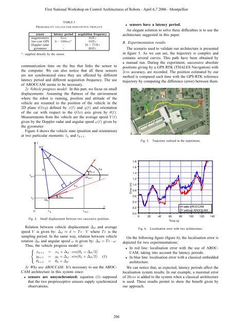
Figure 4 shows the vehicle state (position and orientation)
at two particular moments: tk and tk+1.
y k+1
y
k
O
y
ICC
R
M k
α
x k
θ k
d
∆ d
M k+1
x k+1
θ k+1
∆ θ
Fig. 4. Small displacement between two successive positions.
Relation between vehicle displacement ∆d and average
speed V is given by: ∆d ≈ d = T e · V where T e is the
sampling period. In the same way, relation between vehicle
rotation ∆θ and angular speed ω is given by: ∆θ = T e · ω.
Thus, the vehicle progress model is:
⎧
⎨
⎩
First National Workshop on Control Architectures of Robots - April 6,7 2006 - Montpellier
xk+1 = xk + ∆d · cos(θk + ∆θ/2)
yk+1 = yk + ∆d · sin(θk + ∆θ/2)
θk+1 = θk + ∆θ
3) Why use AROCCAM: It’s necessary to use the AROC-
CAM architecture in this system since:
• sensors are unsynchronized: equation (1) supposed
that the two proprioceptive sensors supply synchronized
observations.
x
(1)
206
• sensors have a latency period.
An elegant solution to solve these difficulties is to use the
architecture suggested in this paper.
B. Experimentation results
The scenario used to validate our architecture is presented
in figure 5. As we can see, the trajectory is complex and
contains several curves. This path have been obtained by
a manual run. During the experiment, successive absolute
positions giving by a GPS RTK (THALES Navigation) with
2cm accuracy, are recorded. The position estimated by our
method is compared each time with the GPS-RTK reference
trajectory by computing the difference (error) between them.
Error (m)
1.8
1.6
1.4
1.2
1.0
0.8
0.6
0.4
End
Fig. 5. Trajectory realised in the experiment.
Begin
0.2
0.0
with AROCCAM
without AROCCAM
0 20 40 60 80 100 120 140
Time (s)
Fig. 6. Localisation error with two architectures.
On the following figure (figure 6), the localisation error is
depicted for two experimentations:
• In red line: localisation error with the use of AROC-
CAM, taking into account the latency periods.
• In blue line: localisation error with a classical embedded
architecture.
We can notice that, as expected, latency periods affect the
localisation system results. In our example, a maximal error
of 20cm is added to the system when a classical architecture
is used. These results permit to show the benefit given by
our approach.