3 - World Journal of Gastroenterology

More documents

Recommendations

Info

B Power (a.u.) 7.6 A Gauthier M et al . Variability of perfusion parameters using DCE-US Attenuated part 1030 930 830 730 630 530 430 0 10 20 30 40 t /s injections of SonoVue ® according to the methodology used in our lab. Settings: During the experiments, mice were placed on the left flank and maintained at a constant temperature through a warming pad (TEM, Bordeaux, France) connected to a Gaymar T/Pump ® (Gaymar Industries, Inc., USA). The temperature was regulated with the adjustable thermostat of the pump and was set at 40°C (internal mouse temperature: 39℃). Each mouse was weighed and the tumor volume was determined before each DCE- US exam. The ROI was set to exclusively include the tumor (Figure 5B-C). An ROI was drawn for each of the repeated measurements and once it was selected, the ultrasound scanner directly allowed access to the time intensity curve associated with the selected ROI. The linear raw data to be modeled were converted through text files and extracted to obtain a graph using Excel ® (Figure 5D). A break of at least 15 min was observed between each injection in addition to 3 min of insonation at a high mechanical index (MI = 1.4), so that contrast agent could be eliminated. Mice were kept asleep no more than 2 h. This duration included the time required for the mice to obtain a stationary heart rate after the administration of anesthesia, acquisition time and the duration of the break WJR|www.wjgnet.com 5 fps VRh5.8 9.2 MI 0.1 Linear raw data Figure 4 Dialyzer. A: Image extracted from an acquisition obtained after a bolus injection of SonoVue ® . As in the case of the first two phantoms, harmonic imaging was based on the Vascular Recognition Imaging mode. The region of interest contained the upper part of the dialyzer to avoid attenuation phenomena in the lower parts. This was manually drawn for each injection; B: To determine perfusion parameters from the time intensity curve obtained following the selection of the region of interest, this was converted through text files so that the analysis could be performed using the Solver program in Excel ® . between each injection. Three injections per mouse were considered for the data analysis. Mice underwent either chemical or gaseous anesthesia. Chemical anesthesia: The amount of chemical anesthesia was determined based upon mouse body weight. Once weighed, the required amount of anesthesia was prepared and injected intraperitoneally using the 1-mL syringe and a “30Gx1/2” needle (Microlance, Ireland). The solution consisted of ketamine (10 mg/mL, Ketalar ® , Parapharm, France) and xylazine (2%, Rompun ® , Bayer, France). To ensure that the mice remained asleep throughout the experiment, 150 µL/g per mouse were systematically injected. Gaseous anesthesia: Mice were anaesthetized through a 2 L/min inhalation of O2 combined with 2.5% of isoflurane. It was possible to modify the flow rate during the experiment so that mice could be maintained asleep without being endangered throughout the experiment. US protocol: Preliminary fundamental B-mode imaging using a 14 MHz PLT 1204AT (Toshiba, Japan) probe was performed to determine the tumor volume prior to the SonoVue ® injection (Figure 5B). The largest longitudinal and transversal sections allowed us to determine the tumor volume by measuring the three perpendicular tumor diameters [26] according to the following formula: V = 1/2 × (depth × width × length). Harmonic imaging was performed in the same way as for the in vitro experiments with a mechanical index set at 0.1 and a rate of 5 fps. Acquisitions lasting 3 min were recorded allowing visualization of both the wash-in and wash-out parts of the TICs. Data analysis As already described in the literature, linear raw data (uncompressed linear data obtained before standard videovisualization) have the advantage of exhibiting a linear dynamic range which is the essential part of the evaluation of semi-quantitative perfusion parameters from TICs [27] . Acquisitions involved recording harmonic images after the SonoVue ® injection, using dedicated software, CHI-Q ® , on the Toshiba Aplio ® ultrasound scanner. In a manually outlined ROI, the mean US signal intensity induced by contrast uptake was obtained and expressed in arbitrary units. This was linearly linked to the number and size of microbubbles in the ROI (Aplio ® procedure) [28,29] . Then, the corresponding TIC to be modeled was converted through text files generated by the ultrasound scanner and extracted to obtain a graph using Excel ® . Seven semi-quantitative perfusion parameters were extracted from this curve: the peak intensity (PI) was the difference between Vmax [maximal intensity value: V(Tmax)] and V0 [Initial intensity value: V(T0)] and represented the highest intensity value attained by the TIC for the defined ROI. The time to peak intensity (TPI), corresponding to Time to Peak Intensity, was the time required for the contrast agent to arrive in the tumor and reach the PI. It 74 March 28, 2011|Volume 3|Issue 3|
D A Power (a.u.) 140 120 100 80 60 40 20 0 0 20 40 60 80 100 120 t /s corresponded to the difference between the latency time (TL), defined as the time between the injection of the product and the beginning of contrast uptake, and Tmax. From a mathematical point of view, TL corresponded to the time at the intersection between y=V0 and the tangent at Tmax/2. The AUC, AUWI and AUWO corresponded to the area under the curve, the area under the wash-in (from T0 to Tmax) and the area under the wash-out (from Tmax to Tend corresponding to the end of the acquisition) of the TIC. The area calculations were based on the trapezoidal rule: the region under the graph of the fitted curve was approximated by trapezoids whose areas were calculated to provide approximations of the areas under the curve, the wash-in or the wash-out. An additional operation of subtracting the offset on the y-axis was performed so that the total area under the curve was independent of it. The limits of integration were defined as follows: [ 0 ] , X ∈ T Tend Where T0 is the initial time. The slope coefficient of the wash-in (WI) was literally defined as the slope of the tangent of the wash-in at half maximum. Finally, the full-width at half maximum (FWHM) was defined as the time interval during which the value of the intensity was higher than Vmax/2. This parameter is commonly considered as a first approximation of the mean transit time (MTT) (Figure 6) [8,26,30] . However, as the linear raw data provided by the ultrasound scanner were too noisy, ex- WJR|www.wjgnet.com B Gauthier M et al . Variability of perfusion parameters using DCE-US 9.11 mm 12.18 mm Linear raw data 7.6 C traction was performed after TIC fitting. This was based on the mathematical model developed at the IGR (Patent: WO/2008/053268 entitled “Method and system for quantification of tumoral vascularization”). 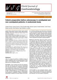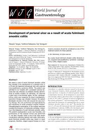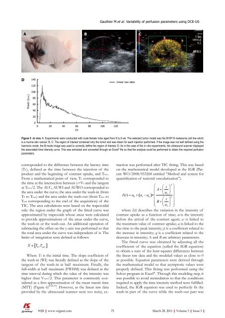p ⎛ ⎞ 5 fps VRh5.8 9.2 Figure 5 In vivo. A: Experiments were conducted with nude female mice aged from 6 to 8 wk. The selected tumor model was the B16F10 melanoma cell line which is a murine skin cancer; B, C: The region of interest contained only the tumor and was drawn for each injection performed. If the image was not well defined using the harmonic mode, the B-mode image was used to correctly define the region of interest; D: As in the case of the in vitro experiments, the ultrasound scanner displayed the associated time intensity curve. This was extracted and converted through an Excel ® file so that the analysis could be performed to obtain the required perfusion parameters. MI 0.1 ⎛ t ⎞ ⎜ A + ⎜ ⎟ ⎟ ⎜ a2 ⎟ I( t) = a0 + ( a1 − a0 ) ∗ ⎝ ⎠ ⎜ q ⎟ ⎜ ⎛ t ⎞ B ⎟ ⎜ + ⎜ ⎟ a ⎟ ⎝ ⎝ 2 ⎠ ⎠ where I(t) describes the variation in the intensity of contrast uptake as a function of time; a0 is the intensity before the arrival of the contrast agent; a1 is linked to the maximum value of contrast uptake; a2 is linked to the rise time to the peak intensity; p is a coefficient related to the increase in intensity; q is a coefficient related to the decrease in intensity; A and B are arbitrary parameters. The fitted curve was obtained by adjusting all the coefficients of the equation (called the IGR equation) to obtain a sum of the least-squares differences between the linear raw data and the modeled values as close to 0 as possible. Equation parameters were derived through the mathematical model so that asymptotic values were properly defined. This fitting was performed using the Solver program in Excel ® . Through this modeling step, it was possible to avoid recirculation so that the conditions required to apply the time intensity method were fulfilled. Indeed, the IGR equation was used to perfectly fit the wash-in part of the curve while the wash-out part was 75 March 28, 2011|Volume 3|Issue 3|
Page 1 and 2: World Journal of Radiology World J
Page 3 and 4: France Alain Chapel, Fontenay-Aux-R
Page 5 and 6: W J R Contents EDITORIAL REVIEW ORI
Page 7 and 8: W J R Online Submissions: http://ww
Page 9 and 10: Rotations Vibrations Water H-bonds
Page 11 and 12: A C D Figure 5 Terahertz imaging of
Page 13 and 14: A Absorption coefficient (cm -1 ) 2
Page 15 and 16: A B Optical delay (ps) 14 12 10 8 6
Page 17 and 18: Pharm Sci 2005; 94: 837-846 44 Mitt
Page 19: to use involved-field radiotherapy
Page 24 and 25: Gauthier M et al . Variability of p
Page 28 and 29: Vmax PI V0 Power (a.u.) 140 120 100
Page 36 and 37: Savini P et al . Extramedullary hae
Page 40 and 41: Instructions to authors in the pape
Page 42 and 43: Instructions to authors PMID and DO

3 - World Journal of Gastroenterology

Create successful ePaper yourself

Delete template?

Save as template?