Non-parametric estimation of a time varying GARCH model

More documents

Recommendations

Info

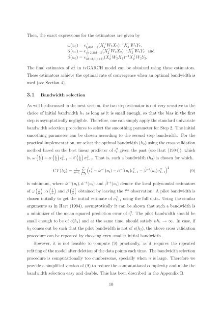
Then, the exact expressions for the estimators are given by ˆω(u0) = e ⊤ 1,3(d+1) (X⊤ 2 W2X2) −1 X ⊤ 2 W2Y2, ˆα(u0) = e ⊤ d+2,3(d+1) (X⊤ 2 W2X2) −1 X ⊤ 2 W2Y2 and ˆβ(u0) = e ⊤ 2d+3,3(d+1) (X⊤ 2 W2X2) −1 X ⊤ 2 W2Y2. The final estimates of σ 2 t in tvGARCH model can be obtained using these estimators. These estimators achieve the optimal rate of convergence when an optimal bandwidth is used (see Section 4). 3.1 Bandwidth selection As will be discussed in the next section, the two step estimator is not very sensitive to the choice of initial bandwidth h1 as long as it is small enough, so that the bias in the first step is asymptotically negligible. Therefore, one can simply apply the standard univariate bandwidth selection procedures to select the smoothing parameter for Step 2. The initial smoothing parameter can be chosen according to the second step bandwidth. For the practical implementation, we select the optimal bandwidth (h2) using the cross validation method based on the best linear predictor of ǫ2 t given the past (see Hart (1994)), which is, ω � � t + α n � � t ǫ n 2 t−1 + β � � t σ n 2 t−1. That is, such a bandwidth (h2) is chosen for which, CV (h2) = 1 n−1 n� t=2 � ǫ2 t − ˆω −t (ut) − ˆα −t (ut)ǫ2 t−1 − ˆ β−t (ut)σ2 �2 t−1 is minimum, where ˆω −t (ut), ˆα −t (ut) and ˆ β−t (ut) denote the local polynomial estimators of ω � � t ,α n � � t and β n � � t obtained by leaving the t n th observation. A pilot bandwidth is chosen initially to get the initial estimate of σ 2 t−1 using the full data. Using the similar arguments as in Hart (1994), asymptotically it can be shown that such a bandwidth is a minimizer of the mean squared prediction error of ǫ 2 t. The pilot bandwidth should be small enough to be of o(h2) and at the same time, should satisfy nh1 → ∞. In case, if h2 comes out be such that the pilot bandwidth is not of o(h2), the above cross validation procedure can be repeated by choosing even smaller initial bandwidth. However, it is not feasible to compute (9) practically, as it requires the repeated refitting of the model after deletion of the data points each time. The bandwidth selection procedure is computationally too cumbersome, specially when n is large. Therefore we provide a simplified version of (9) to reduce the computational complexity and make the bandwidth selection easy and doable. This has been described in the Appendix B. 10 (9)
4 Asymptotic results Towards proving the asymptotic results corresponding to estimators in Steps 1 and 2, we first state the following standard technical assumptions and then introduce some notations: Assumption 2. (i) The functions ω(·),α(·) and β(·) (and hence αj(·)) have the bounded and continuous derivatives up to order d+1 (d ≥ 1), in a neighborhood of u0, u0 ∈ (0, 1]. (ii) K(u) is a symmetric density function of bounded variation with a compact support. (iii) The bandwidths h1 and h2 are such that h1 → 0,h2 → 0 and nh1 → ∞,nh2 → ∞ as n → ∞. (iv) E|vt| 4 < ∞. Notations. µi = � u i K(u)du, νi = � u i K 2 (u)du, S = S(u0) = E � [1, �ǫ 2 t−1(u0),..., �ǫ 2 t−p(u0)] ⊤ [1, �ǫ 2 t−1(u0),..., �ǫ 2 t−p(u0)] � , Cj = Cj(u0) = E(�ǫ 2 t(u0) �ǫ 2 t−j(u0)), Ω = Ω(u0) = E � �σ 4 t (u0)[1, �ǫ 2 t−1(u0),..., �ǫ 2 t−p(u0)] ⊤ [1, �ǫ 2 t−1(u0),..., �ǫ 2 t−p(u0)] � , wj = E(�ǫ j t(u0)), αtvARCH(u0) = [α0(u0),α1(u0),...,αp(u0)] ⊤ , Di = [µd+1,hiµd+2,...,h d iµ2d+1] ⊤ , i = 1, 2, em = a column vector of length m with 1 everywhere, ⎡ ⎢ Ai = ⎢ ⎣ ⎡ ⎢ Bi = ⎢ ⎣ . 1 hiµ1 ... hd iµd hiµ1 h2 iµ2 ... h d+1 ... . . . i µd+1 h d iµd h d+1 i µd+1 ... h 2d i µ2d ν0 hiν1 ... hd iνd hiν1 h2 iν2 ... h d+1 i νd+1 . ... h d iνd h d+1 i νd+1 ... h 2d i ν2d . ⎤ ⎥ ⎦ , ⎤ ⎥ , i = 1, 2. ⎦ In the following theorem, we obtain the exact expressions for the biases of the estimators of tvARCH (p) of Step 1. Theorem 4.1 Let the Assumptions 1 and 2 be satisfied. Then the asymptotic bias of ˆαj(u0), j = 0, 1,...,p is given by, Bias(ˆαj(u0)) = hd+1 � 1 (d+1)! α (d+1) j (u0) � e ⊤ 1,d+1A −1 1 D1 + oP(h d+1 1 ). 11
Page 1 and 2: Non-parametric estimation of a time
Page 3 and 4: 1 Introduction The first decade of
Page 5 and 6: have been discussed in Section 2. S
Page 7 and 8: Under Assumption 1(i), (3) is a sta
Page 9: The estimator of αi(u0) as a solut
Page 13 and 14: Notations. bj = bj(u0) = Bias(ˆαj
Page 15 and 16: This problem is under investigation
Page 17 and 18: provides insight into the nature of
Page 19 and 20: Proof of Proposition 2.3. We can wr
Page 21 and 22: Now consider n� 1 nh k=p+1 (uk
Page 23 and 24: ⎡ X ⊤ ⎢ 1 W1 ⎢ ⎣ and usin
Page 25 and 26: Hence the result can be easily prov
Page 27 and 28: The variance expression given in Th
Page 29 and 30: (iii) a GJR process if where ω,α,
Page 31 and 32: 31 Table 1: Summary statistics of t
Page 33 and 34: 33 Table 3: Aggregated mean squared
Page 35 and 36: −1.5 0.0 1.0 −2 −1 0 1 −1.0
Page 37 and 38: volatility volatility 0 10 20 30 0

Non-parametric estimation of a time varying GARCH model

You also want an ePaper? Increase the reach of your titles

Delete template?

Save as template?