Non-parametric estimation of a time varying GARCH model

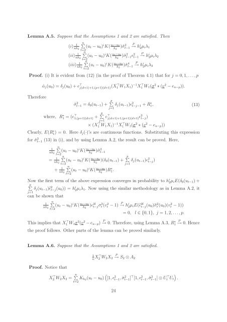
Lemma A.5. Suppose that the Assumptions 1 and 2 are satisfied. Then
(i) 1
n�
(ut − u0) nh2
t=2
iK( ut−u0)ˆσ
h2
2 P
t−1 → hi 2µiλ1
(ii) 1
n�
(ut − u0) nh2
t=2
iK( ut−u0)ˆσ
h2
2 t−1ǫ2 P
t−1 → hi 2µiλ2
(iii) 1
n�
(ut − u0) nh2
t=2
iK( ut−u0)ˆσ
h2
4 P
t−1 → hi 2µiλ3
Proof. (i) It is evident from (12) (in the proof of Theorem 4.1) that for j = 0, 1,...,p
Therefore
ˆαj(u0) = δj(u0) + e ⊤ j(d+1)+1,(p+1)(d+1) (X⊤ 1 W1X1) −1 X ⊤ 1 W1(σ 2 ∗ (v 2 − en−p)).
ˆσ 2 t−1 = δ0(ut−1) + p �
δj(ut−1)ǫ2 t−j−1 + R∗ 1, (13)
where, R ∗ 1 = (e ⊤ 1,(p+1)(d+1) + p �
j=1
e
j=1
⊤ j(d+1)+1,(p+1)(d+1) ǫ2t−j) × (X⊤ 1 W1X1) −1X ⊤ 1 W1(σ2 ∗ (v2 − en−p))
Clearly, E(R ∗ 1) = 0. Here δj(·)’s are continuous functions. Substituting this expression
for ˆσ 2 t−1 (13) in (i), and by using Lemma A.2, the result can be proved. Here,
n� 1 (ut − u0) nh2
t=2
iK( ut−u0)ˆσ
h2
2 t−1
= 1
n�
(ut − u0) nh2
t=2
iK( ut−u0)(δ0(ut−1)
+ h2
p �
δj(ut−1)ǫ
j=1
2 t−j)
+ 1
n�
(ut − u0) nh2
t=2
iK( ut−u0)R
h2
∗ 1.
Now the first term of the above expression converges in probability to hi 2µiE(δ0(ut−1) +
p�
δj(ut−1)�ǫ 2 t−j(u0)) = hi 2µiλ1. Now using the similar methodology as in Lemma A.2, it
j=1
can be shown that
n�
(ut − u0) iK( ut−u0)ǫ2l
t−jσ2 t (v2 t − 1) P → hi 2µiE(�ǫ 2l
t−j(u0)�σ 2 t (u0)(v2 t − 1))
1
nh2
t=2
h2
= 0, l ∈ {0, 1}, j = 1, 2,...,p.
This implies that X ⊤ 1 W1σ 2 (v 2 − en−p) P → 0. Therefore, using Lemma A.3, R ∗ 1
the proof follows. Other parts of the lemma can be proved similarly.
Lemma A.6. Suppose that the Assumptions 1 and 2 are satisfied.
Proof. Notice that
X ⊤ 2 W2X2 = n�
t=2
1
n X⊤ 2 W2X2
P
→ S2 ⊗ A2
Kh2(ut − u0) �
[1,ǫ2 t−1, ˆσ 2 t−1] ⊤ [1,ǫ2 t−1, ˆσ 2 t−1] ⊗ U ⊤ �
t Ut .
24
P
→ 0. Hence