Non-parametric estimation of a time varying GARCH model

each the estimators of the parameter functions of tvGARCH. It has been shown that
with appropriately chosen bandwidth, the rate of convergence of the MSE of final esti-
mates become independent of the initial step estimates.
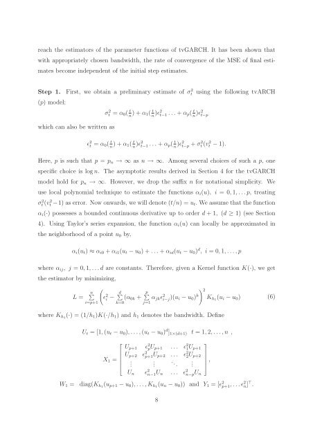
Step 1. First, we obtain a preliminary estimate of σ 2 t using the following tvARCH
(p) model;
which can also be written as
σ2 t = α0( t t ) + α1( n n )ǫ2t−1 ... + αp( t
n )ǫ2t−p ǫ2 t = α0( t t ) + α1( n n )ǫ2t−1 ... + αp( t
n )ǫ2t−p + σ2 t (v2 t − 1).
Here, p is such that p = pn → ∞ as n → ∞. Among several choices of such a p, one
specific choice is log n. The asymptotic results derived in Section 4 for the tvGARCH
model hold for pn → ∞. However, we drop the suffix n for notational simplicity. We
use local polynomial technique to estimate the functions αi(u), i = 0, 1,...p, treating
σ 2 t (v 2 t −1) as error. Now onwards, we will denote (t/n) = ut. We assume that the function
αi(·) possesses a bounded continuous derivative up to order d + 1, (d ≥ 1) (see Section
4). Using Taylor’s series expansion, the function αi(u) can locally be approximated in
the neighborhood of a point u0 by,
αi(ut) ≈ αi0 + αi1(ut − u0) + ... + αid(ut − u0) d , i = 0, 1,...,p
where αij, j = 0, 1,...d are constants. Therefore, given a Kernel function K(·), we get
the estimator by minimizing,
L = n�
�
ǫ
i=p+1
2 i − d�
(α0k +
k=0
p �
αjkǫ
j=1
2 i−j)(ui − u0) k
�2 where Kh1(·) = (1/h1)K(·/h1) and h1 denotes the bandwidth. Define
Ut = [1, (ut − u0),...,(ut − u0) d ]1×(d+1) t = 1, 2,...,n ,
⎡
⎢
X1 = ⎢
⎣
Up+1 ǫ 2 pUp+1 ... ǫ 2 1Up+1
Up+2 ǫ 2 p+1Up+2 ... ǫ 2 2Up+2
.
.
...
Un ǫ 2 n−1Un ... ǫ 2 n−pUn
.
⎤
Kh1(ui − u0) (6)
W1 = diag(Kh1(up+1 − u0),...,Kh1(un − u0)) and Y1 = [ǫ 2 p+1,...ǫ 2 n] ⊤ .
8
⎥
⎦ ,