Convergencia y existencia de la serie de Fourier
Convergencia y existencia de la serie de Fourier
Convergencia y existencia de la serie de Fourier

Create successful ePaper yourself
Turn your PDF publications into a flip-book with our unique Google optimized e-Paper software.
A<br />
<strong>Convergencia</strong> y <strong>existencia</strong> <strong>de</strong> <strong>la</strong> <strong>serie</strong> <strong>de</strong><br />
<strong>Fourier</strong><br />
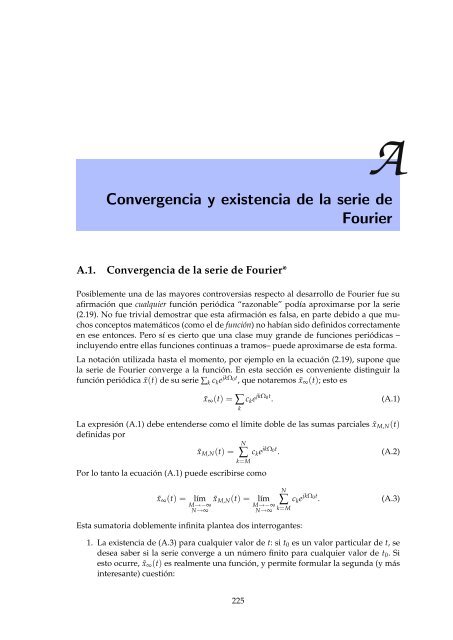
A.1. <strong>Convergencia</strong> <strong>de</strong> <strong>la</strong> <strong>serie</strong> <strong>de</strong> <strong>Fourier</strong>*<br />
Posiblemente una <strong>de</strong> <strong>la</strong>s mayores controversias respecto al <strong>de</strong>sarrollo <strong>de</strong> <strong>Fourier</strong> fue su<br />
afirmación que cualquier función periódica “razonable” podía aproximarse por <strong>la</strong> <strong>serie</strong><br />
(2.19). No fue trivial <strong>de</strong>mostrar que esta afirmación es falsa, en parte <strong>de</strong>bido a que muchos<br />
conceptos matemáticos (como el <strong>de</strong> función) no habían sido <strong>de</strong>finidos correctamente<br />
en ese entonces. Pero sí es cierto que una c<strong>la</strong>se muy gran<strong>de</strong> <strong>de</strong> funciones periódicas –<br />
incluyendo entre el<strong>la</strong>s funciones continuas a tramos– pue<strong>de</strong> aproximarse <strong>de</strong> esta forma.<br />
La notación utilizada hasta el momento, por ejemplo en <strong>la</strong> ecuación (2.19), supone que<br />
<strong>la</strong> <strong>serie</strong> <strong>de</strong> <strong>Fourier</strong> converge a <strong>la</strong> función. En esta sección es conveniente distinguir <strong>la</strong><br />
función periódica ˜x(t) <strong>de</strong> su <strong>serie</strong> ∑k c ke jkΩ0t , que notaremos ˜x∞(t); esto es<br />
˜x∞(t) = ∑ k<br />
c ke jkΩ0t . (A.1)<br />
La expresión (A.1) <strong>de</strong>be enten<strong>de</strong>rse como el límite doble <strong>de</strong> <strong>la</strong>s sumas parciales ˜xM,N(t)<br />
<strong>de</strong>finidas por<br />
N<br />
˜xM,N(t) = ∑ cke k=M<br />
jkΩ0t<br />
. (A.2)<br />
Por lo tanto <strong>la</strong> ecuación (A.1) pue<strong>de</strong> escribirse como<br />
˜x∞(t) = lím ˜xM,N(t) = lím<br />
M→−∞<br />
N→∞<br />
M→−∞<br />
N→∞<br />
N<br />
∑<br />
k=M<br />
Esta sumatoria doblemente infinita p<strong>la</strong>ntea dos interrogantes:<br />
c ke jkΩ0t . (A.3)<br />
1. La <strong>existencia</strong> <strong>de</strong> (A.3) para cualquier valor <strong>de</strong> t: si t0 es un valor particu<strong>la</strong>r <strong>de</strong> t, se<br />
<strong>de</strong>sea saber si <strong>la</strong> <strong>serie</strong> converge a un número finito para cualquier valor <strong>de</strong> t0. Si<br />
esto ocurre, ˜x∞(t) es realmente una función, y permite formu<strong>la</strong>r <strong>la</strong> segunda (y más<br />
interesante) cuestión:<br />
225
226 A. <strong>Convergencia</strong> y <strong>existencia</strong> <strong>de</strong> <strong>la</strong> <strong>serie</strong> <strong>de</strong> <strong>Fourier</strong><br />
2. La i<strong>de</strong>ntidad <strong>de</strong> <strong>la</strong> función periódica ˜x(t) y su <strong>serie</strong> <strong>de</strong> <strong>Fourier</strong> ˜x∞(t). Si <strong>la</strong> <strong>serie</strong><br />
converge a ˜x(t) significa que<br />
˜x∞(t) = lím ˜xM,N(t) = ˜x(t) para todo t.<br />
M→−∞<br />
N→∞<br />
Si <strong>la</strong> <strong>serie</strong> no converge, significa que existen puntos ti tal que<br />
˜x∞(t) = lím ˜xM,N(t) = ˜x(ti).<br />
M→−∞<br />
N→∞<br />
El siguiente teorema, clásico <strong>de</strong>l análisis <strong>de</strong> <strong>Fourier</strong>, resuelve estas inquietu<strong>de</strong>s.<br />
Teorema 1. Teorema básico <strong>de</strong> convergencia puntual. Si ˜x(t) es una señal periódica,<br />
continua a tramos y suave a tramos sobre un intervalo (a, b), entonces:<br />
si ˜x( · ) es continua en t0 ∈ (a, b), sx(t0) converge a ˜x(t0); esto es<br />
N<br />
lím ∑<br />
N→∞<br />
k=−N<br />
∑ k<br />
c ke jkΩ0t0 = ˜x(t0).<br />
si ˜x( · ) tiene una discontinuidad tipo salto en t0 ∈ (a, b),<br />
cke jkΩ0t0<br />
<br />
1<br />
=<br />
2<br />
lím<br />
t→t − 0<br />
˜x(t) + lím<br />
t→t + 0<br />
El teorema establece que <strong>la</strong> <strong>serie</strong> <strong>de</strong> <strong>Fourier</strong> compleja <strong>de</strong> una función periódica se comporta<br />
“a<strong>de</strong>cuadamente”, al menos sobre intervalos don<strong>de</strong> <strong>la</strong> función es continua y suave<br />
a tramos. En cada punto <strong>de</strong> ese intervalo <strong>la</strong> <strong>serie</strong> converge exactamente al valor <strong>de</strong> <strong>la</strong><br />
función en ese punto (por eso se dice que <strong>la</strong> convergencia es puntual). En aquellos puntos<br />
don<strong>de</strong> <strong>la</strong> función presenta saltos (finitos, porque se exige que sea suave a tramos) se tiene<br />
una convergencia simétrica <strong>de</strong> <strong>la</strong> <strong>serie</strong> al valor medio <strong>de</strong> los límites a izquierda y a <strong>de</strong>recha<br />
<strong>de</strong> <strong>la</strong> función en el punto <strong>de</strong> discontinuidad. Gráficamente, este valor es el punto medio<br />
<strong>de</strong>l salto. La convergencia simétrica se entien<strong>de</strong> en el sentido que <strong>la</strong> variable k tien<strong>de</strong> a<br />
(+∞) y a (−∞) a <strong>la</strong> misma velocidad.<br />
El Teorema 1 muestra que siempre que ˜x( · ) sea suave a tramos y periódica, <strong>la</strong> función<br />
˜x( · ) y <strong>la</strong> <strong>serie</strong> <strong>de</strong> <strong>Fourier</strong> ˜x∞(t) representan <strong>la</strong> misma función continua a tramos sobre<br />
toda <strong>la</strong> línea real, confirmando <strong>la</strong> conjetura <strong>de</strong> <strong>Fourier</strong> para el caso en que <strong>la</strong> función es<br />
continua a tramos y periódica. Este es un resultado importante (y famoso), y también se<br />
enuncia como un teorema.<br />
Teorema 2. I<strong>de</strong>ntidad <strong>de</strong> <strong>la</strong>s funciones y su <strong>serie</strong> <strong>de</strong> <strong>Fourier</strong> (versión 1). Si ˜x( · ) es<br />
una función periódica, suave a tramos sobre R, y ˜x∞( · ) su <strong>serie</strong> <strong>de</strong> <strong>Fourier</strong>, entonces<br />
˜x∞(t) converge en cada punto don<strong>de</strong> ˜x( · ) es continua, y<br />
˜x(t) = ˜x∞(t)<br />
en cada punto t don<strong>de</strong> ˜x( · ) es continua. <br />
Procesamiento Digital <strong>de</strong> Señales U.N.S. 2011<br />
˜x(t)
A.1. <strong>Convergencia</strong> <strong>de</strong> <strong>la</strong> <strong>serie</strong> <strong>de</strong> <strong>Fourier</strong>* 227<br />
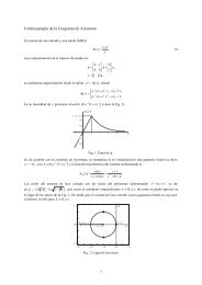
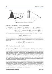
Fig. A.1. Señal diente <strong>de</strong> sierra <strong>de</strong>l Ejemplo A.1.<br />
EJEMPLO A.1. Diente <strong>de</strong> sierra<br />
La <strong>serie</strong> <strong>de</strong> <strong>Fourier</strong> <strong>de</strong> <strong>la</strong> función diente <strong>de</strong> sierra ˜x(t) <strong>de</strong> período T = 3, <strong>de</strong>finida en un período<br />
como ˜x(t) = t con 0 < t < 3, como se muestra en <strong>la</strong> Fig. A.1, está dada por<br />
˜x∞(t) = 3<br />
2 −<br />
∞<br />
∑<br />
k=−∞<br />
k=0<br />
3<br />
2πk jej2π k 3 t .<br />
Este función es suave a tramos en toda <strong>la</strong> línea real, y es continua en todo t salvo cuando t es<br />
múltiplo <strong>de</strong> T = 3. El Teorema 2 asegura que <strong>la</strong> <strong>serie</strong> ˜x∞(t) converge para todo t que no sea<br />
múltiplo <strong>de</strong> 3. Por ejemplo, para t = t0 = 3/4, ˜x(t0) = 3/4, y<br />
˜x∞(t)| t= 3 4<br />
= 3<br />
2 −<br />
= 3<br />
2 −<br />
∞<br />
∑<br />
k=−∞<br />
k=0<br />
∞<br />
∑<br />
k=1<br />
3<br />
2πk jej2π k 3 3 4 = 3<br />
2 −<br />
∞<br />
∑<br />
k=1<br />
3<br />
3<br />
j(2j) sen(πk/2) =<br />
2πk<br />
3<br />
2πk j(ejπk/2 − e −jπk/2 )<br />
2 +<br />
Como sen(πk/2) = 0 para k par, se reemp<strong>la</strong>za k = 2r + 1, y entonces<br />
sx(t)| t= 3 4<br />
= 3<br />
2 +<br />
= 3<br />
2 +<br />
∞<br />
∑<br />
r=0<br />
∞<br />
∑<br />
r=0<br />
3<br />
3<br />
sen[π(2r + 1)/2] =<br />
π(2r + 1)<br />
3<br />
π(2r + 1) (−1)r+1 = 3<br />
4 ,<br />
2 +<br />
∞<br />
∑<br />
k=1<br />
∞<br />
∑<br />
r=0<br />
3<br />
πk sen(πk/2)<br />
3<br />
sen[πr + π/2]<br />
π(2r + 1)<br />
porque ∑ ∞ r=0 3(−1)r+1 /[π(2r + 1)] = −3/4. Por lo tanto, se verifica que ˜x∞(t0) = ˜x(t0), al<br />
menos para un t = t0 que no es múltiplo <strong>de</strong> T = 3.<br />
Por otra parte, ˜x(t) es discontinua en t = nT, n ∈ Z, y por ejemplo en t = t1 = 6, <strong>la</strong> <strong>serie</strong> converge<br />
simétricamente:<br />
N<br />
lím ∑<br />
N→∞<br />
k=−N<br />
cke jkΩ0t0<br />
3<br />
= − lím<br />
2 N→∞<br />
N<br />
∑<br />
k=−N<br />
3<br />
2πk jej2π k 3 6 = 3<br />
− lím<br />
2 N→∞<br />
Sin embargo, no converge en sentido general, ya que,<br />
lím<br />
M→−∞<br />
N→∞<br />
N<br />
∑<br />
k=M<br />
c ke jkΩ0t = 3<br />
2<br />
− lím<br />
M→−∞<br />
N→∞<br />
N<br />
∑<br />
k=M<br />
3<br />
2πk jej2π k 3 6 = 3<br />
2<br />
N<br />
∑<br />
k=0<br />
3<br />
2πk j(ej4πk − e −j4πk ) = 3<br />
2 .<br />
− lím<br />
M→−∞<br />
N→∞<br />
3j<br />
2π<br />
N<br />
1<br />
∑ k<br />
k=M<br />
.<br />
La última expresión es <strong>la</strong> <strong>serie</strong> armónica bilátera que no converge en sentido amplio. <br />
Procesamiento Digital <strong>de</strong> Señales U.N.S. 2011
228 A. <strong>Convergencia</strong> y <strong>existencia</strong> <strong>de</strong> <strong>la</strong> <strong>serie</strong> <strong>de</strong> <strong>Fourier</strong><br />
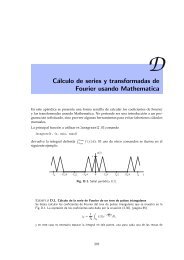
Fig. A.2. Gráfico <strong>de</strong> <strong>la</strong> raíz cuadrada periódica <strong>de</strong>l Ejemplo A.2.<br />
Las funciones periódicas que son suaves a tramos son funciones “razonables” para el<br />
análisis <strong>de</strong> <strong>Fourier</strong>. Como muestra el ejemplo siguiente, muchas función que son “casi”<br />
suaves a tramos también pue<strong>de</strong>n representarse por sus <strong>serie</strong>s <strong>de</strong> <strong>Fourier</strong>.<br />
EJEMPLO A.2. Serie <strong>de</strong> <strong>Fourier</strong> <strong>de</strong> una función que no es suave a tramos<br />
Sea ˜x(t) <strong>la</strong> función periódica <strong>de</strong>finida en un período por ˜x(t) = |t|, para −π < t < π.Esta<br />
función, cuyo gráfico se representa en <strong>la</strong> Fig. A.2, es par, continua, y periódica <strong>de</strong> período 2π. Su<br />
<strong>serie</strong> <strong>de</strong> <strong>Fourier</strong> compleja es <strong>de</strong> <strong>la</strong> forma<br />
˜x∞(t) =<br />
∞<br />
∑<br />
k=−∞<br />
cke jkt , (A.4)<br />
y sus coeficientes c k, cuya expresión analítica no se calcu<strong>la</strong>rá explícitamente, están dados por<br />
ck = 1<br />
π √<br />
−jkt<br />
te dt,<br />
π 0<br />
En t = 0, y por periodicidad en cada t = n2π, con n ∈ Z, no existe <strong>la</strong> <strong>de</strong>rivada <strong>de</strong> ˜x(t):<br />
lím<br />
t→0 +<br />
d ˜x(t)<br />
= lím<br />
dt t→0 +<br />
1<br />
2 √ → ∞,<br />
t<br />
<strong>de</strong> manera que <strong>la</strong> función ˜x(t) no es suave a tramos en cualquier intervalo que contenga un múltiplo<br />
entero <strong>de</strong> 2π, y por lo tanto el Teorema 2 no se pue<strong>de</strong> aplicar.<br />
Sin embargo, cuando t no es un múltiplo entero <strong>de</strong> 2π (por ejemplo en t = 2) existe un intervalo<br />
[por ejemplo (1, 3)] en el cual <strong>la</strong> función ˜x(t) no sólo es suave, sino uniformemente suave. Los<br />
Teoremas 1 y 2 aseguran que <strong>la</strong> <strong>serie</strong> (A.4) converge para t = 2, y que<br />
∞<br />
∑ cke k=−∞<br />
jk2 = ˜x(2) = √ 2.<br />
En general, si t0 es cualquier punto distinto <strong>de</strong> un múltiplo <strong>de</strong> 2π, y τ es <strong>la</strong> distancia entre ese punto<br />
y el múltiplo entero <strong>de</strong> 2π más cercano, resulta que ˜x(t) es uniformemente suave en el intervalo<br />
(t0 − τ/2, t0 + τ/2). Los Teoremas 1 y 2 aseguran que <strong>la</strong> <strong>serie</strong> (A.4) converge para t = t0, y que es<br />
igual a ˜x(t0). Como existe sólo un número finito <strong>de</strong> múltiplos <strong>de</strong> 2π en un intervalo finito cualquiera,<br />
en este intervalo arbitrario <strong>la</strong> función ˜x(t) y su <strong>serie</strong> <strong>de</strong> <strong>Fourier</strong> (A.4) coinci<strong>de</strong>n, y se pue<strong>de</strong> escribir<br />
˜x(t) =<br />
∞<br />
∑ cke k=−∞<br />
jkt ,<br />
don<strong>de</strong> esta igualdad es válida para todo t distinto <strong>de</strong> un múltiplo entero <strong>de</strong> 2π. <br />
Procesamiento Digital <strong>de</strong> Señales U.N.S. 2011
A.2. Aproximaciones uniformes y no uniformes* 229<br />
Bajo <strong>la</strong>s i<strong>de</strong>as ilustradas en el ejemplo anterior se pue<strong>de</strong> probar una versión más general<br />
<strong>de</strong> Teorema 2.<br />
Teorema 3. I<strong>de</strong>ntidad <strong>de</strong> <strong>la</strong>s funciones y su <strong>serie</strong> <strong>de</strong> <strong>Fourier</strong> (versión 2). Sea ˜x(t) una<br />
función continua a tramos, periódica sobre R, y suave a tramos salvo en un número<br />
finito <strong>de</strong> puntos en cada intervalo finito. Entonces <strong>la</strong> <strong>serie</strong> <strong>de</strong> <strong>Fourier</strong> ˜x∞(t) converge<br />
a ˜x(t) en todo el intervalo salvo en un número finito <strong>de</strong> puntos, y por lo tanto ˜x(t) =<br />
˜x∞(t). <br />
De aquí en más se supondrá que <strong>la</strong>s funciones periódicas satisfacen los postu<strong>la</strong>dos <strong>de</strong><br />
los Teoremas 2 o 3, <strong>de</strong> manera que <strong>la</strong> función y su <strong>serie</strong> <strong>de</strong> <strong>Fourier</strong> son representaciones<br />
alternativas <strong>de</strong> un mismo objeto matemático.<br />
A.2. Aproximaciones uniformes y no uniformes*<br />
Efectuar <strong>la</strong> suma infinita indicada en (2.19) o en (A.4) no es conveniente aún con <strong>la</strong>s<br />
mejores computadoras, y en <strong>la</strong> práctica se aproxima ˜x(t) usando una suma parcial ˜xM,N(t),<br />
<strong>de</strong>finida en (A.2) utilizando un número finito <strong>de</strong> términos <strong>de</strong> su <strong>serie</strong> <strong>de</strong> <strong>Fourier</strong> ˜x∞(t).<br />
Para que esta aproximación sea útil, los límites M y N <strong>de</strong>ben elegirse <strong>de</strong> manera que el<br />
error <strong>de</strong> aproximación sea tan pequeño como se <strong>de</strong>see.<br />
Se <strong>de</strong>fine el error en magnitud ˜eM,N(t) a <strong>la</strong> diferencia entre ˜x(t) y su aproximación ˜xM,N(t):<br />
˜eM,N(t) = ˜x(t) − ˜xM,N(t) = ˜x(t) −<br />
N<br />
∑<br />
k=M<br />
c ke jkΩ0t . (A.5)<br />
Evi<strong>de</strong>ntemente, ˜eM,N(t) es una función <strong>de</strong> t. Si ˜x(t) es continua a tramos, el Teorema 1<br />
asegura que para cada t don<strong>de</strong> ˜x(t) es continua,<br />
lím<br />
M→−∞<br />
N→∞<br />
| ˜eM,N(t)| = 0.<br />
Por lo tanto, si ε > 0 es el mayor error <strong>de</strong>seado, y t0 es un punto don<strong>de</strong> ˜x( · ) es continua,<br />
existen números enteros Mε, Nε tales que | ˜eM,N(t0)| < ε cuando M ≥ Mε y N ≥ Nε. Esto<br />
no significa que el error será menor que ε en otros puntos ti = t0. La situación i<strong>de</strong>al sería:<br />
Que para cada ε > 0 existiese un par <strong>de</strong> enteros Mε, Nε tales que | ˜eM,N(t)| < ε para<br />
todo t cuando M ≥ Mε y N ≥ Nε.<br />
Po<strong>de</strong>r <strong>de</strong>terminar Mε, Nε para cualquier ε > 0 dado.<br />
Si <strong>la</strong> primera condición se verifica para todo ε > 0, se dice que ˜xM,N(t) aproxima uniformemente<br />
a ˜x(t), o que ˜xM,N(t) converge uniformemente a ˜x(t) cuando M → −∞, N → +∞.<br />
En otras pa<strong>la</strong>bras, si ˜xM,N(t) es una aproximación uniforme <strong>de</strong> ˜x(t), siempre es posible<br />
encontrar enteros Mε, Nε <strong>la</strong> que <strong>la</strong> suma parcial ˜xM,N(t) difiere <strong>de</strong> ˜x(t) en menos <strong>de</strong> ε para<br />
todo t ∈ R.<br />
Procesamiento Digital <strong>de</strong> Señales U.N.S. 2011
230 A. <strong>Convergencia</strong> y <strong>existencia</strong> <strong>de</strong> <strong>la</strong> <strong>serie</strong> <strong>de</strong> <strong>Fourier</strong><br />
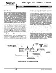
Fig. A.3. Aproximación continua ˜xM,N(t) a una función ˜x(t) con una discontinuidad tipo salto<br />
en t0.<br />
Si una <strong>serie</strong> <strong>de</strong> <strong>Fourier</strong> converge uniformemente a una función, entonces también converge<br />
puntualmente a esa función en toda <strong>la</strong> línea real; esto es<br />
˜x(t) = lím<br />
M→−∞<br />
N→∞<br />
N<br />
∑<br />
k=M<br />
c ke jkΩ0t para todo t ∈ R.<br />
A<strong>de</strong>más, si <strong>la</strong> convergencia es uniforme, el máximo error en usar ∑ N k=M c ke jkΩ0t para calcu<strong>la</strong>r<br />
˜x(t) <strong>de</strong>be ten<strong>de</strong>r a cero cuando M, N tien<strong>de</strong>n a −∞, +∞ respectivamente. Aunque<br />
sin duda esta es <strong>la</strong> situación i<strong>de</strong>al, no siempre ocurre, como se verá a continuación.<br />
A.3. Continuidad y aproximación uniforme*<br />
Cada una <strong>de</strong> <strong>la</strong>s sumas parciales ˜xM,N(t) = ∑ N k=M c ke jkΩ0t <strong>de</strong>be ser una función continua<br />
porque es una suma finita <strong>de</strong> funciones continuas. Por ello es sencillo <strong>de</strong>mostrar que<br />
estas sumas parciales no pue<strong>de</strong>n aproximarse a ˜x(t) <strong>de</strong> manera uniforme si ˜x(t) no es<br />
una función continua. De hecho, si ˜x(t) tiene una discontinuidad tipo salto, para cada<br />
suma parcial ˜xM,N(t) <strong>de</strong>be existir un intervalo (aN, bN) don<strong>de</strong> el error | ˜eM,N(t)| es <strong>de</strong>l<br />
or<strong>de</strong>n <strong>de</strong> <strong>la</strong> mitad <strong>de</strong>l salto. Esta es <strong>la</strong> situación que se presenta en <strong>la</strong> Fig. A.3. Si t0 es<br />
el punto don<strong>de</strong> <strong>la</strong> función ˜x(t) es discontinua, y si ˜xM,N(t) aproxima a ˜x(t) por el <strong>la</strong>do<br />
izquierdo <strong>de</strong> <strong>la</strong> discontinuidad, entonces al ser continua necesita un cierto intervalo para<br />
volver a aproximarse a ˜x(t) a <strong>la</strong> <strong>de</strong>recha <strong>de</strong> <strong>la</strong> discontinuidad. Estos resultados se pue<strong>de</strong>n<br />
formalizar en el siguiente Teorema.<br />
Teorema 4. <strong>Convergencia</strong> uniforme. Sea ˜x( · ) una función periódica continua a tramos.<br />
Si <strong>la</strong> <strong>serie</strong> <strong>de</strong> <strong>Fourier</strong> truncada ˜xM,N( · ) aproxima uniformemente a ˜x( · ), entonces<br />
˜x( · ) <strong>de</strong>be ser una función continua sobre <strong>la</strong> línea real. Recíprocamente, si ˜x( · ) no<br />
es una función continua, entonces ˜xM,N( · ) no aproxima uniformemente a ˜x( · ). Más<br />
aún, si ˜x( · ) tiene una discontinuidad tipo salto <strong>de</strong> amplitud h0 en t = t0, entonces<br />
para cada par <strong>de</strong> enteros M, N, con M < N existe un intervalo (a, b) conteniendo t0 (o<br />
con t0 siendo uno <strong>de</strong> sus extremos) sobre el cual<br />
| ˜x(t) − ˜xM,N(t)| > ρh0,<br />
para todo t ∈ (a, b), y ρ < 1/2. <br />
Procesamiento Digital <strong>de</strong> Señales U.N.S. 2011
A.4. <strong>Convergencia</strong> en norma* 231<br />
Siguiendo estas líneas, el siguiente Teorema confirma que <strong>la</strong> <strong>serie</strong> <strong>de</strong> <strong>Fourier</strong> <strong>de</strong> señales<br />
periódicas continuas converge uniformemente.<br />
Teorema 5. <strong>Convergencia</strong> uniforme. Sea ˜x( · ) una función periódica suave a tramos<br />
con período T. Si ˜x( · ) a<strong>de</strong>más es continua, entonces su <strong>serie</strong> <strong>de</strong> <strong>Fourier</strong> ∑ ∞ k=−∞ cke jkΩ0t<br />
converge uniformemente a ˜x( · ). A<strong>de</strong>más, para cualquier valor t y cualquier par <strong>de</strong><br />
enteros M, N, con M < 0 < N,<br />
don<strong>de</strong><br />
<br />
<br />
<br />
| ˜eM,N(t)| = ˜x(t) −<br />
<br />
N<br />
∑<br />
k=M<br />
cke jkΩ0t<br />
<br />
<br />
<br />
<br />
≤<br />
B = 1<br />
T<br />
T<br />
2π 0<br />
<br />
(−M) −1/2 + (N) −1/2<br />
B<br />
<br />
d ˜x(t)<br />
2<br />
1/2<br />
dt dt<br />
Estos teoremas no aseguran que <strong>la</strong> <strong>serie</strong> <strong>de</strong> <strong>Fourier</strong> <strong>de</strong> ˜x( · ) converge a ˜x( · ) cuando ˜x( · )<br />
sólo es una función periódica continua (pero no suave a tramos). De hecho, existen funciones<br />
periódicas continuas que no se pue<strong>de</strong>n aproximar uniformemente por su <strong>serie</strong> <strong>de</strong><br />
<strong>Fourier</strong>. Estas señales son difíciles <strong>de</strong> construir y no suelen aparecer en <strong>la</strong>s aplicaciones.<br />
A.4. <strong>Convergencia</strong> en norma*<br />
Se dice que una aproximación con un número finito <strong>de</strong> términos ˜xM,N(t) converge en norma<br />
a <strong>la</strong> función ˜x(t) si y sólo si<br />
<br />
<br />
<br />
lím ˜x(t) − c<br />
<br />
ke jkΩ0t<br />
<br />
<br />
<br />
= lím ˜eM,N(t) = 0, (A.6)<br />
<br />
M→−∞<br />
N→∞<br />
N<br />
∑<br />
k=M<br />
M→−∞<br />
N→∞<br />
don<strong>de</strong> ˜eM,N(t) es el error <strong>de</strong>finido en (A.5), y <strong>la</strong> función norma f ( · ) se <strong>de</strong>fine como<br />
f ( · ) 2 = 1<br />
Las expresiones (A.6) son equivalentes a<br />
lím<br />
M→−∞<br />
N→∞<br />
1<br />
T0<br />
T0<br />
0<br />
T0<br />
<br />
<br />
˜x(t) − ∑ N<br />
k=M cke jkΩ0t<br />
<br />
<br />
T0<br />
2<br />
0<br />
| f (t)| 2 dt.<br />
= lím<br />
M→−∞<br />
N→∞<br />
De acuerdo a <strong>la</strong> c<strong>la</strong>sificación <strong>de</strong>l Capítulo 1, <strong>la</strong> expresión<br />
EM,N = 1<br />
T0<br />
T0<br />
0<br />
| ˜eM,N(t)| 2 dt = 1<br />
1<br />
T0<br />
T0<br />
0<br />
| ˜eM,N(t)| 2 dt = 0.<br />
T0<br />
˜eM,N(t) ˜e<br />
T0 0<br />
∗ M,N(t) dt, (A.7)<br />
representa <strong>la</strong> energía promedio <strong>de</strong> <strong>la</strong> señal durante un período, o bien el promedio <strong>de</strong> <strong>la</strong><br />
señal error elevada al cuadrado: el error cuadrático medio.<br />
Procesamiento Digital <strong>de</strong> Señales U.N.S. 2011
232 A. <strong>Convergencia</strong> y <strong>existencia</strong> <strong>de</strong> <strong>la</strong> <strong>serie</strong> <strong>de</strong> <strong>Fourier</strong><br />
Si ˜x(t) es periódica, continua y suave a tramos, el Teorema 5 establece que existe un valor<br />
finito <strong>de</strong> B tal que | ˜eM,N(t)| ≤ (−M) −1/2 + (N) −1/2 B para cada t ∈ R y todos los<br />
enteros M, N tales que M < 0 < N. Entonces, el error medio cuadrático verifica<br />
lím<br />
M→−∞<br />
N→∞<br />
1<br />
T0<br />
T0<br />
0<br />
| ˜eM,N(t)| 2 dt < lím<br />
M→−∞<br />
N→∞<br />
lo que prueba el siguiente Teorema:<br />
< lím<br />
M→−∞<br />
N→∞<br />
T0 1<br />
[(−M)<br />
T0 0<br />
−1/2 + (N) −1/2 ] 2 B 2 dt<br />
[(−M) −1/2 + (N) −1/2 ] 2 B 2 = 0,<br />
Teorema 6. <strong>Convergencia</strong> en norma <strong>de</strong> funciones continuas y suaves a tramos. La <strong>serie</strong><br />
<strong>de</strong> <strong>Fourier</strong> <strong>de</strong> una función periódica continua y suave a tramos converge en norma<br />
a dicha función. <br />
En realidad existe un resultado más fuerte, que establece que <strong>la</strong> <strong>serie</strong> <strong>de</strong> <strong>Fourier</strong> <strong>de</strong> una<br />
función continua a tramos converge en norma a <strong>la</strong> función, aún cuando ésta no sea suave<br />
a tramos.<br />
Teorema 7. <strong>Convergencia</strong> en norma <strong>de</strong> funciones continuas a tramos. La <strong>serie</strong> <strong>de</strong><br />
<strong>Fourier</strong> ∑ ∞ k=−∞ c ke jkΩ0t <strong>de</strong> una función periódica ˜x(t) <strong>de</strong> período T0 = 2π/Ω0 continua<br />
a tramos converge en norma a dicha función; a<strong>de</strong>más se verifica que<br />
˜x( · ) 2 = T0<br />
∞<br />
∑<br />
k=−∞<br />
Esta expresión se conoce como igualdad <strong>de</strong> Bessel. <br />
A.5. Aproximación óptima con un número finito <strong>de</strong> términos*<br />
La mejor manera <strong>de</strong> aproximar <strong>la</strong> función periódica ˜x(t) por una suma finita <strong>de</strong> exponenciales<br />
complejas armónicamente re<strong>la</strong>cionadas es encontrar un conjunto <strong>de</strong> coeficientes c k,<br />
k = −N, . . . , N tal que <strong>la</strong> energía promedio por período <strong>de</strong>l error (A.7) sea mínima. Para<br />
simplificar <strong>la</strong> notación respecto a <strong>la</strong> sección anterior, se consi<strong>de</strong>ra que en <strong>la</strong> sumatoria se<br />
toman <strong>la</strong> misma cantidad <strong>de</strong> términos para k > 0 y para k < 0, esto es, se hace M = −N :<br />
. Desarrol<strong>la</strong>ndo (A.7) se tiene que<br />
EN = 1<br />
= 1<br />
T0<br />
T0 0<br />
T0<br />
T0<br />
0<br />
˜xN(t) =<br />
˜eN(t) ˜e ∗ N(t)dt = 1<br />
|c k| 2<br />
N<br />
∑<br />
k=−N<br />
cke jkΩ0t<br />
. (A.8)<br />
T0<br />
T0<br />
0<br />
[ ˜x(t) − ˜xN(t)][ ˜x(t) − ˜xN(t)]) ∗ dt<br />
[ ˜x(t) ˜x ∗ (t) − ˜x(t) ˜x ∗ N(t) − ˜x ∗ (t) ˜xN(t) + ˜xN(t) ˜x ∗ N(t)] dt.<br />
Procesamiento Digital <strong>de</strong> Señales U.N.S. 2011
A.5. Aproximación óptima con un número finito <strong>de</strong> términos* 233<br />
La condición para que el error sea mínimo es que<br />
esto es<br />
0 = 1<br />
T0<br />
= − 1<br />
T0<br />
T0<br />
0<br />
T0<br />
Teniendo en cuenta que<br />
0<br />
∂EN<br />
∂c k<br />
= 0, k = −N, . . . , N<br />
[− ˜x(t) ∂ ˜x∗ N (t)<br />
− ˜x<br />
∂ck ∗ ∂ ˜xN(t)<br />
(t) +<br />
∂ck ∂ ˜xN(t)<br />
˜x<br />
∂ck ∗ N(t) + ˜xN(t) ∂ ˜x∗ N (t)<br />
] dt<br />
∂ck <br />
[ ˜x(t) − ˜xN(t)] ∂ ˜x∗ N (t)<br />
+ [ ˜x<br />
∂ck ∗ (t) − ˜x ∗ <br />
∂ ˜xN(t)<br />
N(t)] dt (A.9)<br />
∂ck ∂ ˜xN(t)<br />
∂c k<br />
= e jkΩ0t , y que<br />
∂ ˜x ∗ N (t)<br />
∂c k<br />
= 0,<br />
pues ˜x ∗ N (t) <strong>de</strong>pen<strong>de</strong> <strong>de</strong> c∗ k , pero no <strong>de</strong> c k, <strong>la</strong> expresión (A.9) se pue<strong>de</strong> escribir como<br />
0 = 1<br />
= 1<br />
= 1<br />
T0<br />
T0 0<br />
T0<br />
T0 0<br />
T0<br />
T0<br />
0<br />
[ ˜x ∗ (t) − ˜x ∗ ∂ ˜xN(t)<br />
N(t)] dt =<br />
∂ck 1<br />
<br />
<br />
˜x ∗ (t) −<br />
N<br />
∑<br />
ℓ=−N<br />
˜x ∗ (t)e jkΩ0t dt − 1<br />
c ∗ ℓ e−jℓΩ0t<br />
T0<br />
T0<br />
0<br />
T0<br />
T0<br />
0<br />
[ ˜x ∗ (t) − ˜x ∗ N(t)]e jkΩ0t dt<br />
e jkΩ0t dt (A.10)<br />
N<br />
∑<br />
ℓ=−N<br />
c ∗ ℓ ej(k−ℓ)Ω0t dt. (A.11)<br />
(note el cambio <strong>de</strong> variable k por ℓ en <strong>la</strong> sumatoria para evitar confusiones son el índice<br />
k <strong>de</strong>l c k respecto al cual se está <strong>de</strong>rivando.) Por <strong>la</strong> propiedad <strong>de</strong> ortogonalidad <strong>de</strong> <strong>la</strong>s<br />
exponenciales complejas (nota al pie <strong>de</strong> <strong>la</strong> página 74)<br />
1<br />
T0<br />
T0<br />
0<br />
N<br />
∑ c<br />
ℓ=−N<br />
∗ ℓ ej(k−ℓ)Ω0t N T0 1<br />
dt = ∑ c<br />
T0 ℓ=−N 0<br />
∗ ℓ ej(k−ℓ)Ω0t ∗<br />
dt = cℓ . (A.12)<br />
Finalmente, <strong>de</strong> (A.11) y (A.12), y conjugando y renombrando los índices, se encuentra<br />
que<br />
ck = 1<br />
T0<br />
˜x(t)e −jkΩ0t<br />
dt, k = −N, . . . , N. (A.13)<br />
T0<br />
0<br />
En otras pa<strong>la</strong>bras, los coeficientes (A.13) que minimizan <strong>la</strong> integral <strong>de</strong>l error entre ˜x(t) y<br />
su aproximación ˜xN(t) <strong>de</strong> or<strong>de</strong>n N son los mismos coeficientes <strong>de</strong> <strong>la</strong> <strong>serie</strong> <strong>de</strong> <strong>Fourier</strong> (2.20):<br />
si <strong>la</strong> señal ˜x(t) admite una representación en <strong>serie</strong>s <strong>de</strong> <strong>Fourier</strong>, <strong>la</strong> mejor aproximación<br />
usando una suma finita <strong>de</strong> exponenciales complejas armónicamente re<strong>la</strong>cionadas es <strong>la</strong><br />
que se obtiene truncando <strong>la</strong> <strong>serie</strong> <strong>de</strong> <strong>Fourier</strong> al número <strong>de</strong> términos <strong>de</strong>seados. A medida<br />
que se incrementa N, se agregan nuevos términos, pero los anteriores permanecen sin<br />
cambios, y EN <strong>de</strong>crece. De hecho, si ˜x(t) tiene una representación en <strong>serie</strong>s <strong>de</strong> <strong>Fourier</strong>,<br />
lím<br />
N→∞ EN = 0.<br />
En otras pa<strong>la</strong>bras, el error medio cuadrático entre <strong>la</strong> función ˜x(t) y su representación<br />
˜xN(t) formada por un número finito <strong>de</strong> términos <strong>de</strong> <strong>la</strong> <strong>serie</strong> <strong>de</strong> <strong>Fourier</strong> es nulo. Esto no<br />
significa que <strong>la</strong>s funciones sean iguales, como se comenta en <strong>la</strong> siguiente sección.<br />
Procesamiento Digital <strong>de</strong> Señales U.N.S. 2011
234 A. <strong>Convergencia</strong> y <strong>existencia</strong> <strong>de</strong> <strong>la</strong> <strong>serie</strong> <strong>de</strong> <strong>Fourier</strong><br />
A.6. Vali<strong>de</strong>z <strong>de</strong> <strong>la</strong> representación en <strong>serie</strong>s <strong>de</strong> <strong>Fourier</strong>*<br />
Dada una señal periódica ˜x(t) siempre se pue<strong>de</strong> intentar obtener un conjunto <strong>de</strong> coeficientes<br />
<strong>de</strong> <strong>Fourier</strong> a partir <strong>de</strong> <strong>la</strong> ecuación (2.20). Sin embargo, en algunos casos <strong>la</strong> integral<br />
pue<strong>de</strong> no converger (el valor <strong>de</strong> alguno <strong>de</strong> los c k pue<strong>de</strong> ser infinito), y en otros, aún cuando<br />
todos los c k sean finitos, <strong>la</strong> sustitución <strong>de</strong> estos coeficientes en <strong>la</strong> ecuación <strong>de</strong> síntesis<br />
(2.19) pue<strong>de</strong> no converger a <strong>la</strong> señal original ˜x(t).<br />
Si <strong>la</strong> señal ˜x(t) es continua no hay problemas <strong>de</strong> convergencia: toda función periódica<br />
continua tiene una representación en <strong>serie</strong>s <strong>de</strong> <strong>Fourier</strong> <strong>de</strong> modo que <strong>la</strong> energía <strong>de</strong>l error<br />
<strong>de</strong> aproximación (A.7) tien<strong>de</strong> a cero a medida que N → ∞. Esto también es cierto para<br />
muchas señales discontinuas. Como éstas son muy comunes en el estudio <strong>de</strong> señales<br />
y sistemas –por ejemplo, el tren <strong>de</strong> pulsos rectangu<strong>la</strong>res <strong>de</strong>l Ejemplo 2.4– es necesario<br />
analizar <strong>la</strong> convergencia con más <strong>de</strong>talle. Al discutir estas condiciones no se intenta una<br />
justificación matemática rigurosa, <strong>la</strong> que pue<strong>de</strong> encontrarse en otros textos sobre análisis<br />
<strong>de</strong> <strong>Fourier</strong> (Churchill, 1963; Kap<strong>la</strong>n, 1962).<br />
Una c<strong>la</strong>se <strong>de</strong> señales periódicas que son representables con <strong>la</strong>s <strong>serie</strong>s <strong>de</strong> <strong>Fourier</strong> compren<strong>de</strong><br />
<strong>la</strong>s funciones <strong>de</strong> cuadrado integrable sobre un período. Estas señales tienen energía<br />
finita sobre un período, <br />
| ˜x(t)| 2 dt < ∞,<br />
T<br />
<strong>de</strong> don<strong>de</strong> los coeficientes c k calcu<strong>la</strong>dos con (2.20) son finitos. Si ˜xN(t) representa <strong>la</strong> aproximación<br />
a ˜x(t) usando 2N + 1 términos <strong>de</strong> <strong>la</strong> <strong>serie</strong> <strong>de</strong> <strong>Fourier</strong> como en <strong>la</strong> ecuación (A.8),<br />
se pue<strong>de</strong> probar que el error medio cuadrático EN <strong>de</strong>finido por (A.7) tien<strong>de</strong> a cero cuando<br />
N tien<strong>de</strong> a infinito. Es <strong>de</strong>cir, si<br />
e(t) = ˜x(t) −<br />
entonces <br />
T<br />
+∞<br />
∑<br />
k=−∞<br />
|e(t)| 2 dt = 0.<br />
c ke jk2π f t ,<br />
Esta ecuación no significa que <strong>la</strong>s señal ˜x(t) y su representación en <strong>serie</strong> <strong>de</strong> <strong>Fourier</strong><br />
+∞<br />
∑ cke k=−∞<br />
jk2π f t , (A.14)<br />
son iguales en todo instante <strong>de</strong> tiempo t; lo que dice es que no hay energía en <strong>la</strong> diferencia<br />
entre <strong>la</strong>s dos. Las funciones como <strong>la</strong>s indicadas al pie <strong>de</strong> <strong>la</strong> página 79 son diferentes, pero<br />
tienen <strong>la</strong> misma representación en <strong>serie</strong>s <strong>de</strong> <strong>Fourier</strong>. El error entre <strong>la</strong> función y <strong>la</strong> <strong>serie</strong><br />
sólo es nulo para ˜x2(t). Para ˜x1(t) y ˜x3(t) el error e(t) es nulo para todo t cuando N → ∞,<br />
excepto para t = ±τ/2 + kT0, k ∈ Z, don<strong>de</strong> |eN(t)| = 1/2 para cualquier N. Sin embargo,<br />
para cada valor <strong>de</strong> N el error medio cuadrático EN <strong>de</strong>finido por (A.7) es el mismo para<br />
<strong>la</strong>s tres funciones.<br />
El tipo <strong>de</strong> convergencia garantizado cuando x(t) es <strong>de</strong> cuadrado integrable es muy útil<br />
en el tratamiento <strong>de</strong> señales y sistemas. La mayoría <strong>de</strong> <strong>la</strong>s señales con que se trabaja en<br />
este campo tiene energía finita sobre un período, y por lo tanto admiten representación<br />
en <strong>serie</strong>s <strong>de</strong> <strong>Fourier</strong>. Si bien ˜xN(t) y ˜x(t) no son idénticas en todos los puntos, el hecho<br />
Procesamiento Digital <strong>de</strong> Señales U.N.S. 2011
A.6. Vali<strong>de</strong>z <strong>de</strong> <strong>la</strong> representación en <strong>serie</strong>s <strong>de</strong> <strong>Fourier</strong>* 235<br />
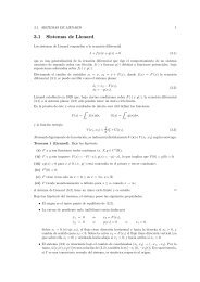
Fig. A.4. Funciones que no satisfacen <strong>la</strong>s condiciones <strong>de</strong> Dirichlet.<br />
que <strong>la</strong> diferencia entre ambas tenga energía nu<strong>la</strong> cuando N → ∞ es muy conveniente en<br />
muchas aplicaciones. Se suele <strong>de</strong>cir que ˜xN(t) aproxima en mínimos cuadrados a ˜x(t).<br />
P. L. Dirichlet enunció un conjunto <strong>de</strong> condiciones –que también son satisfechas por casi<br />
todas <strong>la</strong>s señales <strong>de</strong> interés– que garantiza que ˜x(t) y su <strong>serie</strong> serán idénticas, excepto en el<br />
conjunto <strong>de</strong> puntos en don<strong>de</strong> ˜x(t) es discontinua don<strong>de</strong> <strong>la</strong> <strong>serie</strong> infinita (A.14) converge<br />
al valor medio <strong>de</strong> <strong>la</strong> discontinuidad. Estas condiciones son suficientes pero no necesarias,<br />
lo que significa que existen funciones que pue<strong>de</strong>n no satisfacer alguna <strong>de</strong> el<strong>la</strong>s, pero aún<br />
así tener representación en <strong>serie</strong>s <strong>de</strong> <strong>Fourier</strong>. Las condiciones son:<br />
1. ˜x (t) es absolutamente integrable sobre un período, es <strong>de</strong>cir<br />
<br />
T<br />
| ˜x (t)| dt < ∞. (A.15)<br />
Como suce<strong>de</strong> con <strong>la</strong>s funciones <strong>de</strong> cuadrado integrable sobre un período, esto garantiza<br />
que todos los coeficientes c k son finitos, ya que, <strong>de</strong> acuerdo con (A.15),<br />
|ak| ≤ 1<br />
<br />
<br />
˜x(t) e<br />
T T<br />
−jkω0t<br />
<br />
<br />
dt = 1<br />
<br />
T<br />
T<br />
| ˜x(t)| dt < ∞.<br />
Una señal periódica que vio<strong>la</strong> <strong>la</strong> primera condición <strong>de</strong> Dirichlet es <strong>la</strong> que se presenta<br />
en Fig. A.4(a) , <strong>de</strong>finida como<br />
don<strong>de</strong> ˜x(t) es periódica con período 1.<br />
˜x(t) = 1<br />
, 0 < t ≤ 1,<br />
t<br />
2. ˜x (t) tiene un número finito <strong>de</strong> máximos y mínimos (se dice que es <strong>de</strong> variación<br />
acotada). Un ejemplo <strong>de</strong> una función que verifica <strong>la</strong> condición 1, pero no <strong>la</strong> 2, es<br />
<br />
2π<br />
˜x(t) = sin , 0 < t ≤ 1,<br />
t<br />
que se grafica en <strong>la</strong> Fig. A.4(b) . Esta función, periódica con período T = 1, es absolutamente<br />
integrable<br />
1<br />
0<br />
| ˜x(t)| dt < 1,<br />
pero tiene un número no finito <strong>de</strong> máximos y mínimos en el intervalo.<br />
Procesamiento Digital <strong>de</strong> Señales U.N.S. 2011
236 A. <strong>Convergencia</strong> y <strong>existencia</strong> <strong>de</strong> <strong>la</strong> <strong>serie</strong> <strong>de</strong> <strong>Fourier</strong><br />
3. ˜x (t) tiene un número finito <strong>de</strong> discontinuida<strong>de</strong>s (finitas) en un intervalo finito <strong>de</strong><br />
tiempo. Una función que vio<strong>la</strong> esta condición es <strong>la</strong> que muestra <strong>la</strong> Fig. A.4(c), <strong>de</strong><br />
período T = 8, compuesta <strong>de</strong> un número infinito <strong>de</strong> secciones cada una <strong>de</strong> <strong>la</strong>s<br />
cuales tiene <strong>la</strong> mitad <strong>de</strong> <strong>la</strong> altura y el ancho <strong>de</strong> <strong>la</strong>s secciones previas. Aunque es<br />
absolutamente integrable, pues el área <strong>de</strong>bajo <strong>de</strong> un período es menor que 8, el<br />
número <strong>de</strong> discontinuida<strong>de</strong>s en el período es infinito.<br />
Los ejemplos muestran que <strong>la</strong>s señales que no satisfacen los criterios <strong>de</strong> Dirichlet son generalmente<br />
<strong>de</strong> naturaleza patológica, y en consecuencia no muy importantes en el estudio<br />
<strong>de</strong> señales y sistemas.<br />
Resumiendo, <strong>la</strong> representación en <strong>serie</strong>s <strong>de</strong> <strong>Fourier</strong> <strong>de</strong> señales<br />
continuas converge e igua<strong>la</strong> a <strong>la</strong> señal original en para cada valor <strong>de</strong> t.<br />
discontinuas converge en todo punto salvo en los puntos <strong>de</strong> discontinuidad, don<strong>de</strong><br />
converge al valor medio <strong>de</strong>l salto. En este caso <strong>la</strong> diferencia entre <strong>la</strong> señal original<br />
y <strong>la</strong> representada por <strong>la</strong> <strong>serie</strong> infinita no contiene energía, <strong>de</strong> modo que para todos<br />
los fines prácticos ambas señales son idénticas. Como ambas señales difieren sólo<br />
en puntos ais<strong>la</strong>dos, sus integrales coinci<strong>de</strong>n sobre cualquier intervalo; por ello se<br />
comportan igual bajo <strong>la</strong> convolución y son idénticas <strong>de</strong>s<strong>de</strong> el punto <strong>de</strong> vista <strong>de</strong>l<br />
análisis <strong>de</strong> sistema lineales e invariantes en el tiempo.<br />
Procesamiento Digital <strong>de</strong> Señales U.N.S. 2011