Consulter le texte intégral de la thèse - Université de Poitiers
Consulter le texte intégral de la thèse - Université de Poitiers
Consulter le texte intégral de la thèse - Université de Poitiers

You also want an ePaper? Increase the reach of your titles
YUMPU automatically turns print PDFs into web optimized ePapers that Google loves.
Jury :<br />
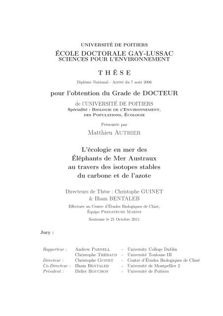
UNIVERSITÉ DE POITIERS<br />
ÉCOLE DOCTORALE GAY-LUSSAC<br />
SCIENCES POUR L’ENVIRONNEMENT<br />
THÈSE<br />
Diplôme National - Arrêté du 7 août 2006<br />
pour l’obtention du Gra<strong>de</strong> <strong>de</strong> DOCTEUR<br />
<strong>de</strong> l’UNIVERSITÉ DE POITIERS<br />
Spécialité : Biologie <strong>de</strong> l’Environnement,<br />
<strong>de</strong>s Popu<strong>la</strong>tions, Écologie<br />
Présentée par<br />
Matthieu Authier<br />
L’écologie en mer <strong>de</strong>s<br />
Éléphants <strong>de</strong> Mer Austraux<br />
au travers <strong>de</strong>s isotopes stab<strong>le</strong>s<br />
du carbone et <strong>de</strong> l’azote<br />
Directeurs <strong>de</strong> Thèse : Christophe GUINET<br />
&IlhamBENTALEB<br />
Effectuée au Centre d’Étu<strong>de</strong>s Biologiques <strong>de</strong> Chizé,<br />
Équipe Predateurs Marins<br />
Soutenue <strong>le</strong> 21 Octobre 2011<br />
Rapporteur : Andrew Parnell - University Col<strong>le</strong>ge Dublin<br />
Christophe Thébaud - <strong>Université</strong> Toulouse III<br />
Directeur : Christophe Guinet - Centre d’Étu<strong>de</strong>s Biologiques <strong>de</strong> Chizé<br />
Co-Directeur : Ilham Benta<strong>le</strong>b - <strong>Université</strong> <strong>de</strong> Montpellier 2<br />
Prési<strong>de</strong>nt : Didier Bouchon - <strong>Université</strong> <strong>de</strong> <strong>Poitiers</strong>
Remerciements<br />
Je remercie Vincent Bretagnol<strong>le</strong>, directeur du Centre d’Étu<strong>de</strong>s Biologiques <strong>de</strong><br />
Chizé, <strong>de</strong> m’avoir accueilli au CEBC et permis d’effectuer ce travail <strong>de</strong> <strong>thèse</strong>.<br />
Je remercie l’Éco<strong>le</strong> Doctora<strong>le</strong> Gay-Lussac et l’<strong>Université</strong> <strong>de</strong> <strong>Poitiers</strong> pour<br />
m’avoir accueilli. Je remercie en particulier Mme Sylvie Perez et Sabrina Biais pour<br />
<strong>le</strong>ur disponibilité et pour avoir toujours facilité <strong>le</strong>s démarches administratives.<br />
Je remercie gran<strong>de</strong>ment Christophe Guinet pour m’avoir encadré et fait<br />
partagé sa passion <strong>de</strong>s mammifères marins. Merci <strong>de</strong> m’avoir repêché et donner<br />
<strong>la</strong> gran<strong>de</strong> chance <strong>de</strong> pouvoir re-faire une <strong>thèse</strong> après mes déboires boréaux. Merci<br />
aussi d’avoir supporté mes sautes d’humeur et mes atermoiements.<br />
Je tiens à remercier Ilham Benta<strong>le</strong>b pour l’accueil à Montpellier ! Merci<br />
aussi à Céline Martin et Aurore Ponchon pour m’avoir ai<strong>de</strong>r à braver <strong>le</strong> micromill.<br />
Je remercie éga<strong>le</strong>ment Olivier Commonwick pour <strong>la</strong> mise en forme L ATEX.<br />
Je remercie éga<strong>le</strong>ment <strong>le</strong>s chercheurs du CEBC en particulier Yves Cherel<br />
et Christophe Barbraud pour <strong>le</strong>urs conseils et <strong>le</strong>ur disponibilité. Merci éga<strong>le</strong>ment à<br />
Dominique Besson, sans qui bien <strong>de</strong>s choses auraient été plus compliquées.<br />
Un merci tout particulier à mon petit JB ! Une bel<strong>le</strong> rencontre, faîte sur<br />
cette bonne î<strong>le</strong> d’Amsterdam, qui dure <strong>de</strong>puis... Peut-être y as tu d’ail<strong>le</strong>urs revu ’<strong>la</strong><br />
masse’ : ce brave petit V976. En tout cas, tu avais encore une fois raison : South<br />
Park pendant <strong>la</strong> rédaction <strong>de</strong> <strong>thèse</strong>, ça ai<strong>de</strong> beaucoup !<br />
Merci aussi à toi C<strong>la</strong>ra, pour toute cette bonne humeur et tout ce ta<strong>le</strong>nt<br />
! Et pour avoir supporté ma maniaquerie (standardise ! ! ! !). Aucun doute que<br />
l’on recroisera encore autour d’une bonne grail<strong>le</strong> ou pour par<strong>le</strong>r RRRRrrrr !<br />
Mil<strong>le</strong>s mercis à toi Quentin pour m’avoir permis <strong>de</strong> squatter ton appart<br />
pendant tout ce temps à Montpellier. Certes, ce<strong>la</strong> s’est payé en soirée tri <strong>de</strong> pelotes<br />
<strong>de</strong> chouettes ! Rhââ ! Et puis surtout merci <strong>de</strong> m’avoir montré comment manipu<strong>le</strong>r<br />
ces grosses bébêtes que sont <strong>le</strong>s Éléphants <strong>de</strong> Mer !<br />
Je ne sais pas non plus comment te remercier Manue pour toutes ces discussions<br />
et toutes ces interactions ! Merci aussi d’avoir été là pendant <strong>le</strong>s pério<strong>de</strong>s<br />
<strong>de</strong> tempêtes... Satanées matrices !
ii<br />
À Aurélie, Vincent, et Annette. Merci <strong>le</strong>s colloques <strong>de</strong> votre soutien et bonne<br />
humeur. Ah ! Annette, <strong>le</strong> potager va mal : on aura quand même dû traiter un peu !<br />
Vincent, il me reste encore <strong>de</strong>s soupes en sachets, mais je ne crois pas <strong>le</strong>s boire un<br />
jour, même à ta santé. Aurélie, ton chat fiche <strong>de</strong>s roustes au mien : ça ne va pas du<br />
tout !<br />
Merci à Sophie et Maxime, compagnons <strong>de</strong> galère <strong>de</strong>s <strong>de</strong>rnières heures <strong>de</strong><br />
rédaction. El<strong>le</strong>s sont toujours extra ces petites pauses thé. Et Thibaut, je serai<br />
encore dispo pour plumer un dindon <strong>le</strong>s soirs où tu t’ennuieras ! On ne <strong>la</strong>issera pas<br />
crever <strong>la</strong> vian<strong>de</strong> !<br />
Merci à <strong>la</strong> “Guinet’s Team” : Anne-Céci<strong>le</strong> (à <strong>la</strong> découverte <strong>de</strong>s Éléphants<br />
Mer ! Pas toujours faci<strong>le</strong> mais on en est revenu !), Morgane (bonnes bestio<strong>le</strong>s que tes<br />
otaries), Cédric (alors ça gam ?), Paul (sa<strong>le</strong>s bêtes que tes orques), Flore (dommage<br />
pour <strong>le</strong> <strong>de</strong>rnier Pot-pot...), Adrien, Guil<strong>la</strong>ume, Marie, et Céci<strong>le</strong>.<br />
Merci à <strong>la</strong> Team agropip aussi pour <strong>la</strong> bonne humeur : Boen, Adrien,<br />
Vincent.<br />
Et au fait Amélie, merci encore pour <strong>la</strong> Love room ! On retourne quand<br />
tu veux se baigner dans une eau à 10 ◦ avec Ibou !<br />
Une pensée bien particulière aux gens que je néglige <strong>de</strong>puis trop longtemps<br />
avec mes histoires <strong>de</strong> sciences. En premier lieu mes amis VCAT, Jean-Marie,<br />
Odi<strong>le</strong>, Anne et Vincent (et Manon ! ! !).<br />
À Alicia et Mi<strong>la</strong>, I still treasure your friendship, my preciousss ! J’espère<br />
que Mi<strong>la</strong> se souvient bien <strong>de</strong> comment on fait <strong>la</strong> loutre.<br />
À Paul et C<strong>la</strong>ire, merci d’ouvrir encore votre porte parisienne à ce sauvage<br />
<strong>de</strong>s Deux-Sèvres.<br />
Anaïs, Thomas et Luka.... j’ai honte <strong>de</strong> mon si<strong>le</strong>nce !<br />
Un immense merci à Lusignan : Tata C<strong>la</strong>udie et Tonton Jean-Paul ; Sébastien<br />
(merci <strong>de</strong> subvenir à <strong>la</strong> recherche avec ton jardin !), Florence, Antoine, et<br />
Adè<strong>le</strong> ; Florian, Pauline et Augustin ; Pauline.<br />
Une pensée toute particulière à Joss et Delphin, Cathy et Domi, Xavier,<br />
Christine, Noémie, Aïcha : <strong>la</strong> joyeuse ban<strong>de</strong> du 18 rue Rivals ! Merci <strong>de</strong> ces soirées<br />
incroyab<strong>le</strong>s !
Enfin, merci à mon petit frère, Stéphane et à mes parents, Gérard et Ro<strong>la</strong>n<strong>de</strong><br />
<strong>de</strong> supporter mes longues absences et mes longs si<strong>le</strong>nces <strong>de</strong>puis 10 ans... Je n’aurai<br />
jamais pu faire tout ce que j’ai pu sans votre éternel soutien.<br />
Et merci à toi Grégory, d’être là aujourd’hui et <strong>de</strong>main.<br />
iii
Nous <strong>de</strong>vons toujours nous souvenir que nous n’observons jamais <strong>la</strong> Nature<br />
el<strong>le</strong>-même, mais seu<strong>le</strong>ment cette nature que nos métho<strong>de</strong>s entrevoient.<br />
W. K. Heisenberg (1958)<br />
Il apprit rapi<strong>de</strong>ment bien <strong>de</strong>s choses, et généralisa beaucoup, <strong>de</strong> façon souvent<br />
erronée. [...]. Il s’en tira cependant, à <strong>la</strong> manière <strong>de</strong>s gens <strong>de</strong> son espèce, en<br />
présentant ces généralisations comme <strong>de</strong>s "essais".<br />
Jack London (1909)<br />
’J’ai cru comprendre que vous aviez <strong>de</strong> fortes opinions politiques.’<br />
Je répondis : ’Oh non. Seu<strong>le</strong>ment <strong>de</strong>s opinions extrêmes mol<strong>le</strong>ment maintenues.’<br />
A.P.J. Taylor (1977)<br />
Une autre erreur est <strong>la</strong> colère. Souvent un scientifique se courrouce, sans que ce<strong>la</strong><br />
n’arrange quoi que ce soit. Se divertir, oui, s’énerver, non. La colère touche<br />
rarement sa cib<strong>le</strong>.<br />
R. Hamming (1986)<br />
La spécilisation <strong>de</strong>s science nous a privé d’une gran<strong>de</strong> part <strong>de</strong> notre passion. Nous<br />
voulions saisir <strong>le</strong>s sciences dans <strong>le</strong>ur <strong>intégral</strong>ité, mais cette <strong>intégral</strong>ité était bien<br />
trop vaste et comp<strong>le</strong>xe à harnacher. Bien trop rarement pouvons-nous poser <strong>le</strong>s<br />
questions profon<strong>de</strong>s qui nous ont amenées en premier lieu vers <strong>le</strong>s sciences.<br />
E.P. Wigner<br />
La rage <strong>de</strong> vouloir conclure est une <strong>de</strong>s manies <strong>le</strong>s plus funestes et <strong>le</strong>s plus stéri<strong>le</strong>s<br />
qui appartiennent à l’humanité. Chaque religion, et chaque philosophie, a prétendu<br />
avoir Dieu à el<strong>le</strong>, toiser l’infini et connaître <strong>la</strong> recette du bonheur. Quel orgueil et<br />
quel néant !<br />
G. F<strong>la</strong>ubert (1863)<br />
v
Tab<strong>le</strong> <strong>de</strong>s matières<br />
1 Introduction 1<br />
1.1 Écologie Alimentaire . . . . . . . . . . . . . . . . . . . . . . . . . . . 2<br />
1.2 Étudier <strong>de</strong>s Popu<strong>la</strong>tions Sauvages . . . . . . . . . . . . . . . . . . . . 4<br />
1.2.1 L’Approche dite <strong>de</strong> ’Biologging’ . . . . . . . . . . . . . . . . . 5<br />
1.2.2 Une Approche Indirecte : <strong>le</strong>s Isotopes Stab<strong>le</strong>s . . . . . . . . . 6<br />
1.3 Informations Indirectes . . . . . . . . . . . . . . . . . . . . . . . . . . 8<br />
1.3.1 Un Téléscope pour <strong>le</strong>s Écologues . . . . . . . . . . . . . . . . 8<br />
1.3.2 Le Statisticien comme Interprète . . . . . . . . . . . . . . . . 9<br />
1.4 Objectifs <strong>de</strong> cette Thèse . . . . . . . . . . . . . . . . . . . . . . . . . 11<br />
1.4.1 Cyc<strong>le</strong> Biologique <strong>de</strong>s Éléphants <strong>de</strong> Mer . . . . . . . . . . . . . 13<br />
1.4.2 Synopsis <strong>de</strong> <strong>la</strong> Thèse . . . . . . . . . . . . . . . . . . . . . . . 17<br />
2 Tendance Actuel<strong>le</strong> <strong>de</strong> <strong>la</strong> Popu<strong>la</strong>tion 19<br />
2.1 Estimation <strong>de</strong> <strong>la</strong> Tail<strong>le</strong> <strong>de</strong> <strong>la</strong> Popu<strong>la</strong>tion . . . . . . . . . . . . . . . . 20<br />
2.1.1 Dénombrement <strong>de</strong>s Femel<strong>le</strong>s Reproductrices . . . . . . . . . . 20<br />
2.1.2 Asynchronie dans <strong>la</strong> Reproduction . . . . . . . . . . . . . . . 20<br />
2.2 Modélisation Hiérarchique . . . . . . . . . . . . . . . . . . . . . . . . 21<br />
2.2.1 Présence à Terre <strong>de</strong>s Femel<strong>le</strong>s Reproductrices . . . . . . . . . 21<br />
2.2.2 Partition <strong>de</strong> <strong>la</strong> Variance . . . . . . . . . . . . . . . . . . . . . 23<br />
2.2.3 Pic <strong>de</strong> Présence et Synchronie . . . . . . . . . . . . . . . . . . 24<br />
2.3 Correction <strong>de</strong>s Dénombrements . . . . . . . . . . . . . . . . . . . . . 28<br />
2.3.1 Phénoménologie <strong>de</strong> <strong>la</strong> Reproduction . . . . . . . . . . . . . . 29<br />
2.3.2 Tendance Popu<strong>la</strong>tionnel<strong>le</strong> . . . . . . . . . . . . . . . . . . . . 30<br />
3 Quête Alimentaire 33<br />
3.1 Zones d’Alimentation . . . . . . . . . . . . . . . . . . . . . . . . . . . 33<br />
3.2 Isotopes Stab<strong>le</strong>s et Télémétrie . . . . . . . . . . . . . . . . . . . . . . 37<br />
3.2.1 Analyse <strong>de</strong>s Trajets . . . . . . . . . . . . . . . . . . . . . . . 37<br />
3.2.2 Résolution Temporel<strong>le</strong> . . . . . . . . . . . . . . . . . . . . . . 37<br />
3.2.3 Cartographie Isotopique <strong>de</strong> l’Océan Austral . . . . . . . . . . 42<br />
3.3 Stratégies Maternel<strong>le</strong>s . . . . . . . . . . . . . . . . . . . . . . . . . . 47<br />
3.3.1 Proxy <strong>de</strong> <strong>la</strong> Va<strong>le</strong>ur Sé<strong>le</strong>ctive . . . . . . . . . . . . . . . . . . . 47<br />
3.3.2 Récolte <strong>de</strong>s Données . . . . . . . . . . . . . . . . . . . . . . . 48<br />
3.3.3 Isotopes Stab<strong>le</strong>s du Sang . . . . . . . . . . . . . . . . . . . . . 49<br />
3.3.4 Stratégie Maternel<strong>le</strong> d’Approvisionnement . . . . . . . . . . . 51<br />
3.3.5 Conditions Environnementa<strong>le</strong>s . . . . . . . . . . . . . . . . . 59<br />
3.4 Discussion . . . . . . . . . . . . . . . . . . . . . . . . . . . . . . . . . 64
viii Tab<strong>le</strong> <strong>de</strong>s matières<br />
4 Quête Alimentaire et Histoire <strong>de</strong> Vie 67<br />
4.1 Ontogénie <strong>de</strong> <strong>la</strong> Quête Alimentaire . . . . . . . . . . . . . . . . . . . 68<br />
4.1.1 Données Transverva<strong>le</strong>s . . . . . . . . . . . . . . . . . . . . . . 68<br />
4.1.2 Niveau Trophique <strong>de</strong>s Éléphants <strong>de</strong> Mer . . . . . . . . . . . . 72<br />
4.2 Données Longitudina<strong>le</strong>s . . . . . . . . . . . . . . . . . . . . . . . . . 75<br />
4.3 Changements Ontogénétiques . . . . . . . . . . . . . . . . . . . . . . 76<br />
4.3.1 Col<strong>le</strong>cte <strong>de</strong>s Données . . . . . . . . . . . . . . . . . . . . . . . 76<br />
4.3.2 Modè<strong>le</strong>s à Point <strong>de</strong> Rupture . . . . . . . . . . . . . . . . . . . 78<br />
4.3.3 Formu<strong>la</strong>tion Hiérarchique . . . . . . . . . . . . . . . . . . . . 80<br />
4.3.4 Résultats . . . . . . . . . . . . . . . . . . . . . . . . . . . . . 81<br />
4.4 Quête Alimentaire et Longévité . . . . . . . . . . . . . . . . . . . . . 88<br />
4.4.1 Longévité dans <strong>la</strong> Nature . . . . . . . . . . . . . . . . . . . . 88<br />
4.4.2 Modèlisation Jointe Données Longitudina<strong>le</strong>s/Survie ...... 89<br />
4.4.3 Résultats . . . . . . . . . . . . . . . . . . . . . . . . . . . . . 92<br />
4.4.4 Conséquences à Long Terme <strong>de</strong> <strong>la</strong> Vie Juvéni<strong>le</strong> . . . . . . . . 94<br />
5 Discussion Fina<strong>le</strong> 97<br />
5.1 Information Indirecte . . . . . . . . . . . . . . . . . . . . . . . . . . . 98<br />
5.2 Isotopes Stab<strong>le</strong>s et Modè<strong>le</strong>s à Mé<strong>la</strong>nge . . . . . . . . . . . . . . . . . 100<br />
5.3 Quelques Limites <strong>de</strong>s Sources d’Informations Indirectes . . . . . . . . 103<br />
5.4 Perspectives . . . . . . . . . . . . . . . . . . . . . . . . . . . . . . . . 106<br />
A Statistiques Bayésiennes 109<br />
B Métho<strong>de</strong>s du Chapitre 2 113<br />
B.1 Priors . . . . . . . . . . . . . . . . . . . . . . . . . . . . . . . . . . . 113<br />
B.2 Distributions Alternatives au Prior Wishart Inverse . . . . . . . . . . 114<br />
C Métho<strong>de</strong>s du Chapitre 3 121<br />
C.1 Analyses en Laboratoire . . . . . . . . . . . . . . . . . . . . . . . . . 121<br />
C.2 Analyses Statistiques . . . . . . . . . . . . . . . . . . . . . . . . . . . 122<br />
C.2.1 Résolution Temporel<strong>le</strong> . . . . . . . . . . . . . . . . . . . . . . 122<br />
C.2.2 Cartographie Isotopique <strong>de</strong> l’Océan Austral . . . . . . . . . . 122<br />
C.2.3 Stratégie Maternel<strong>le</strong> d’Approvisionnement . . . . . . . . . . . 124<br />
C.2.4 Se<strong>le</strong>ction du Modè<strong>le</strong> à Mé<strong>la</strong>nge . . . . . . . . . . . . . . . . . 124<br />
C.2.5 Une Fonction <strong>de</strong> Lien Robuste : <strong>le</strong> Robit . . . . . . . . . . . . 125<br />
D Métho<strong>de</strong>s du Chapitre 4 129<br />
D.1 Analyses <strong>de</strong> Laboratoire . . . . . . . . . . . . . . . . . . . . . . . . . 129<br />
D.1.1 Analyse du Sang . . . . . . . . . . . . . . . . . . . . . . . . . 129<br />
D.1.2 Analyse <strong>de</strong>s Dents . . . . . . . . . . . . . . . . . . . . . . . . 130<br />
D.2 Données Transversa<strong>le</strong>s . . . . . . . . . . . . . . . . . . . . . . . . . . 132<br />
D.3 Modè<strong>le</strong> à Point <strong>de</strong> Rupture Hiérarchique . . . . . . . . . . . . . . . . 132<br />
D.3.1 Priors . . . . . . . . . . . . . . . . . . . . . . . . . . . . . . . 132<br />
D.3.2 Sé<strong>le</strong>ction et Ajustement <strong>de</strong>s Modè<strong>le</strong>s . . . . . . . . . . . . . . 133
Tab<strong>le</strong> <strong>de</strong>s matières ix<br />
D.4 Modè<strong>le</strong> Joint Point <strong>de</strong> Rupture/Survie . . . . . . . . . . . . . . . . . 138<br />
D.4.1 Priors . . . . . . . . . . . . . . . . . . . . . . . . . . . . . . . 138<br />
D.4.2 Vérification <strong>de</strong> l’Ajustement . . . . . . . . . . . . . . . . . . . 138<br />
D.4.3 Stochastic Search Variab<strong>le</strong> Se<strong>le</strong>ction . . . . . . . . . . . . . . 139<br />
Bibliographie 143
Chapitre 1<br />
Introduction<br />
Contents<br />
1.1 Écologie Alimentaire ....................... 2<br />
1.2 Étudier <strong>de</strong>s Popu<strong>la</strong>tions Sauvages ............... 4<br />
1.2.1 L’Approche dite <strong>de</strong> ’Biologging’ . . . . . . . . . . . . . . . . . 5<br />
1.2.2 Une Approche Indirecte : <strong>le</strong>s Isotopes Stab<strong>le</strong>s . . . . . . . . . 6<br />
1.3 Informations Indirectes ...................... 8<br />
1.3.1 Un Téléscope pour <strong>le</strong>s Écologues . . . . . . . . . . . . . . . . 8<br />
1.3.2 Le Statisticien comme Interprète . . . . . . . . . . . . . . . . 9<br />
1.4 Objectifs <strong>de</strong> cette Thèse ..................... 11<br />
1.4.1 Cyc<strong>le</strong> Biologique <strong>de</strong>s Éléphants <strong>de</strong> Mer . . . . . . . . . . . . 13<br />
1.4.2 Synopsis <strong>de</strong> <strong>la</strong> Thèse . . . . . . . . . . . . . . . . . . . . . . . 17
2 Chapitre 1. Introduction<br />
1.1 Écologie Alimentaire<br />
Il est entendu par quête alimentaire d’un organisme l’ensemb<strong>le</strong> <strong>de</strong>s comportements<br />
et <strong>de</strong>s capacités à acquérir et assimi<strong>le</strong>r <strong>de</strong>s ressources dont l’utilisation ultérieure<br />
déterminera <strong>la</strong> va<strong>le</strong>ur se<strong>le</strong>ctive, ou aptitu<strong>de</strong> biologique, <strong>de</strong> cet organisme. Les<br />
patrons d’utilisation <strong>de</strong> ces ressources se traduisent en patrons d’histoire <strong>de</strong> vie<br />
via <strong>le</strong> processus d’allocation (Boggs, 1992; Stearns, 1989). Alors que l’allocation<br />
<strong>de</strong>s ressources à différentes fonctions biologiques est un processus intra-individuel,<br />
<strong>la</strong> quête alimentaire est quant-à-el<strong>le</strong> un processus inter-individuel (Graphique<br />
1.1). Lorsque <strong>le</strong>s ressources sont limitées, <strong>le</strong>s organismes <strong>de</strong>vront faire face à<br />
<strong>de</strong>s compromis d’allocation : par exemp<strong>le</strong> allouer temps et énergie à <strong>la</strong> reproduction<br />
peut entraîner une réduction <strong>de</strong>s ressources dévouées à <strong>la</strong> croissance<br />
somatique ou <strong>la</strong> survie (Pianka, 1976; Stearns, 1989). La quête alimentaire est<br />
donc crucia<strong>le</strong> puisqu’el<strong>le</strong> détermine dans quel<strong>le</strong> mesure <strong>le</strong>s organismes feront face<br />
à <strong>de</strong> tels compromis, soit parce que certaines ressources clés sont limitées dans<br />
l’environnement, soit parce que <strong>le</strong>s individus diffèrent <strong>de</strong> par <strong>le</strong>ur capacité à<br />
acquérir et extraire <strong>le</strong>s ressources (vanNoordwijkand<strong>de</strong>Jong, 1986). Alors que <strong>la</strong><br />
compétition inter-individuel<strong>le</strong> décou<strong>le</strong> d’une limitation globa<strong>le</strong> <strong>de</strong>s ressources, une<br />
capacité différentiel<strong>le</strong> à extraire <strong>le</strong>s ressources du milieu ne présuppose pas que ces<br />
ressources soient limitées. De tel<strong>le</strong>s différences pourraient dés lors refléter <strong>la</strong> qualité<br />
<strong>de</strong>s individus, qualité signifiant ici un trait phénotypique, donc observab<strong>le</strong>, corrélé<br />
<strong>de</strong> manière positive à <strong>la</strong> va<strong>le</strong>ur se<strong>le</strong>ctive (Cam et al., 2002; Bergeron et al., 2011).<br />
Cette re<strong>la</strong>tion étroite entre quête alimentaire et traits d’histoire <strong>de</strong> vie préconise<br />
<strong>de</strong> connaître dans <strong>le</strong> détail l’écologie alimentaire <strong>de</strong>s organismes afin <strong>de</strong><br />
comprendre <strong>le</strong>s conséquences popu<strong>la</strong>tionnel<strong>le</strong>s <strong>de</strong>s différents patrons d’histoire <strong>de</strong><br />
vie (Co<strong>le</strong>, 1954). Néanmoins, un tel <strong>de</strong>grés <strong>de</strong> détail est diffici<strong>le</strong> à obtenir et <strong>le</strong><br />
problème est fondamenta<strong>le</strong>ment hiérarchique puisque qu’il résulte <strong>de</strong> l’interaction<br />
entre un niveau individuel (allocation) et un niveau popu<strong>la</strong>tionnel (compétition)<br />
(Robinson, 2009; Cooch et al., 2002). Ainsi que <strong>le</strong> soulignent <strong>le</strong>s bouc<strong>le</strong>s <strong>de</strong><br />
rétroaction du Graphique 1.1, <strong>de</strong>s données sur <strong>le</strong>s processus à <strong>la</strong> fois intra- et<br />
inter-individuel sont nécessaires pour une compréhension exhaustive <strong>de</strong> <strong>la</strong> quête<br />
alimentaire.
1.1. Écologie Alimentaire 3<br />
Reproduction<br />
Inter-Individus<br />
Ressources<br />
disponib<strong>le</strong>s<br />
dans<br />
l’Environnement<br />
Quête<br />
Alimentaire<br />
Ressources<br />
disponib<strong>le</strong>s<br />
dans<br />
l’Organisme<br />
Intra-Individu<br />
Allocation<br />
Stockage<br />
Croissance/Maintenance<br />
somatique<br />
Survie<br />
Fig. 1.1 – Niveaux d’analyse et interaction entre quête alimetaire et allocation<br />
(modifié <strong>de</strong> Boggs (1992). Dans <strong>le</strong> cas d’organismes avec une phase <strong>de</strong> dormance<br />
ou une stratégie <strong>de</strong> reproduction sur capital, il existe un déca<strong>la</strong>ge temporel entre<br />
acquisition et utilisation <strong>de</strong>s ressources extraites du milieu.
4 Chapitre 1. Introduction<br />
1.2 Étudier <strong>de</strong>s Popu<strong>la</strong>tions Sauvages<br />
Dans <strong>le</strong> milieu naturel, <strong>le</strong>s ressources environnementa<strong>le</strong>s fluctuent généra<strong>le</strong>ment<br />
autant dans l’espace que dans <strong>le</strong> temps (Boggs, 1992). Une tel<strong>le</strong> hétérogénéité<br />
structure <strong>la</strong> ’scène écologique’ sur <strong>la</strong>quel<strong>le</strong> <strong>le</strong>s organismes évoluent. La quête<br />
alimentaire peut ainsi être appréhendée comme un problème d’optimisation :<br />
puisque l’environnement au sens <strong>la</strong>rge, c’est-à-dire biotique et abiotique, impose<br />
certaines contraintes, comment <strong>le</strong>s organismes s’adaptent-ils à ces contraintes pour<br />
une efficacité maxima<strong>le</strong> <strong>de</strong>s comportements <strong>de</strong> quête alimentaire ? L’efficacité peut<br />
se définir comme un taux d’énergie (ressources) extraite par unité <strong>de</strong> temps. Un<br />
lien causal entre aptitu<strong>de</strong> biologique (<strong>la</strong> capacité <strong>de</strong>s organismes à survivre et à<br />
contribuer <strong>de</strong>s <strong>de</strong>scendants viab<strong>le</strong>s à <strong>la</strong> génération suivante) et efficacité est alors<br />
supposé exister. Cette secon<strong>de</strong> hypo<strong>thèse</strong> (<strong>la</strong> première étant que <strong>le</strong>s organismes sont<br />
décrits adéquatement comme agents maximisateurs d’une fonction d’utilité) est <strong>le</strong><br />
plus souvent nécessaire pour contourner l’épineux problème d’estimer directement<br />
une aptitu<strong>de</strong> biologique (Link et al., 2002; Metcalf and Parvard, 2006). L’aptitu<strong>de</strong><br />
biologique est communément définie comme <strong>la</strong> monnaie <strong>de</strong> <strong>la</strong> sé<strong>le</strong>ction naturel<strong>le</strong>,<br />
c’est-à-dire comme un trait <strong>la</strong>tent (ou inobservab<strong>le</strong> directement, peut-être même<br />
un trait multi-dimensionel) indiquant <strong>le</strong> taux <strong>de</strong> propagation <strong>de</strong> génotypes au<br />
cours <strong>de</strong>s générations (Link et al., 2002). Cette définition est rétrospective et rend<br />
diffici<strong>le</strong> 1 l’estimation d’une aptitu<strong>de</strong> biologique pour <strong>de</strong>s individus encore vivants,<br />
qui ne se sont pas encore reproduits, etc.<br />
La théorie <strong>de</strong> l’Approvisionnement Optimal (’Optimal foraging theory’, MacArthur<br />
and Pianka (1966)) utilise ainsi un critère d’optimalité pour juger <strong>le</strong><br />
mérite d’une stratégie <strong>de</strong> quête alimentaire par rapport à une autre. Dans ce cadre<br />
conceptuel, <strong>la</strong> quête alimentaire <strong>de</strong> plusieurs organismes contemporains peut donc<br />
être mesurée et comparée en terme d’efficacité. Toutefois, même en <strong>la</strong>issant <strong>de</strong><br />
côté <strong>le</strong>s problèmes philosophiques sous-jacent aux approches d’optimisation en<br />
biologie (par exemp<strong>le</strong> Gould and Lewontin (1979); Sakar (2005); Depew (2010)), <strong>le</strong><br />
biologiste <strong>de</strong> terrain continue <strong>de</strong> faire face à <strong>de</strong>s problèmes pratiques pour mesurer<br />
in natura <strong>le</strong>s comportements <strong>de</strong> recherche alimentaires d’animaux sauvages.<br />
1 mais non impossib<strong>le</strong> pour autant (Link et al., 2002; Link and Barker, 2009)
1.2. Étudier <strong>de</strong>s Popu<strong>la</strong>tions Sauvages 5<br />
1.2.1 L’Approche dite <strong>de</strong> ’Biologging’<br />
Les chal<strong>le</strong>nges posés par l’étu<strong>de</strong> d’animaux sauvages dans <strong>le</strong>ur milieu naturel se sont<br />
érodés au cours <strong>de</strong>s 20 <strong>de</strong>rnières années durant <strong>le</strong>squel<strong>le</strong>s l’utilisation d’enregistreurs<br />
miniatures posés directement sur <strong>le</strong>s organismes s’est considérab<strong>le</strong>ment développée<br />
(voir par exemp<strong>le</strong>, Péron et al. (2010)) pour aboutir à ce qui est communément<br />
appelé <strong>la</strong> “révolution du biologging” (Ropert-Cou<strong>de</strong>rt and Wilson, 2005). Par <strong>le</strong><br />
biais <strong>de</strong> métho<strong>de</strong>s télémétriques et d’analyses <strong>de</strong> trajectoire, <strong>la</strong> quête alimentaire<br />
s’infère à partir <strong>de</strong>s mouvements dans l’espace <strong>de</strong>s animaux sauvages (Jonsen<br />
et al., 2007; Patterson et al., 2008) même si, dans <strong>la</strong> plupart <strong>de</strong>s cas, <strong>la</strong> nature<br />
<strong>de</strong>s ressources consommées n’est pas directement connue (voir Davis et al. (1999)<br />
pour un contre exemp<strong>le</strong>). Ces énormes progrès en miniaturisation signifient qu’il<br />
est désormais possib<strong>le</strong> d’équiper <strong>de</strong>s animaux aux moeurs aussi cryptiques que <strong>de</strong>s<br />
anguil<strong>le</strong>s (Aarestrup et al., 2009) ou <strong>de</strong>s tortues aquatiques (Hart and Fujisaki,<br />
2010). Hebb<strong>le</strong>white and Haydon (2010) discutent <strong>de</strong> manière critique <strong>le</strong>s impressionnants<br />
succés du ’biologging’, et mettent en évi<strong>de</strong>nce plusieurs ang<strong>le</strong>s morts dans<br />
<strong>la</strong> révolution. Avec un ton délibéremment provocateur, Hebb<strong>le</strong>white and Haydon<br />
(2010) haranguent <strong>le</strong>s biologistes <strong>de</strong> distinguer entre ce qui est impressionnant<br />
et ce qui est important au fur et à mesure que grandit ’<strong>la</strong> montagne <strong>de</strong> données<br />
comprenant <strong>de</strong>s millions <strong>de</strong> localisations’. Alors que ces données <strong>de</strong> locations sont<br />
toujours plus nombreuses et précises, <strong>le</strong> nombre d’animaux qui peuvent être ainsi<br />
équipés reste mo<strong>de</strong>ste, sinon faib<strong>le</strong>, d’un point <strong>de</strong> vue statistique (voir Block et al.<br />
(2011) pour un contre-exemp<strong>le</strong>).<br />
Ce <strong>de</strong>rnier point peut poser problème dés lors que l’on souhaite généraliser<br />
un patron observé sur un échantillon à l’ensemb<strong>le</strong> <strong>de</strong> <strong>la</strong> popu<strong>la</strong>tion. Si aboutir à<br />
<strong>de</strong>s décisions <strong>de</strong> conservation est un <strong>de</strong>s buts <strong>de</strong> l’étu<strong>de</strong> <strong>de</strong> ’biologging’ (Thiebot,<br />
2011), cette capacité à pouvoir généraliser est hautement désirab<strong>le</strong>. Par exemp<strong>le</strong>,<br />
Wakefield et al. (2011) ont analysé <strong>le</strong>s comportements <strong>de</strong> quête alimetaire <strong>de</strong>s Albatros<br />
à Sourcils Noirs (Tha<strong>la</strong>ssarche me<strong>la</strong>nophrys). Leurs inférences concernaient<br />
l’ensemb<strong>le</strong> <strong>de</strong> <strong>la</strong> popu<strong>la</strong>tion mondia<strong>le</strong>, estimée à quelques ≈ 600, 000 coup<strong>le</strong>s, mais<br />
proviennaient d’un échantillon <strong>de</strong> 163 individus suivis sur une pério<strong>de</strong> <strong>de</strong> 10 ans.<br />
Cet exemp<strong>le</strong> illustre que <strong>de</strong>s considérations d’ordre statistique ne peuvent être<br />
faci<strong>le</strong>ment écartées avec l’approche <strong>de</strong> ’biologging’.
6 Chapitre 1. Introduction<br />
1.2.2 Une Approche Indirecte : <strong>le</strong>s Isotopes Stab<strong>le</strong>s<br />
A l’opposé <strong>de</strong> l’approche <strong>de</strong> ’biologging’ en terme <strong>de</strong> coûts financiers, se situe une<br />
approche indirecte consistant à mesurer dans divers échantillons biologiques <strong>le</strong> ratio<br />
naturel d’isotopes stab<strong>le</strong>s d’éléments chimiques (tels <strong>le</strong> carbone, l’azote, <strong>le</strong> soufre,<br />
l’hydrogène, l’oxygène, etc...). En effet, <strong>de</strong>puis <strong>le</strong>s travaux fondateurs <strong>de</strong> DeNiro and<br />
Epstein (1978, 1981) etFry et al. (1978), l’utilisation d’isotopes stab<strong>le</strong>s pour inférer<br />
et révé<strong>le</strong>r <strong>le</strong>s liens écologiques unissant <strong>le</strong>s espèces est allée grandissante en écologie<br />
(West et al., 2006). Ces premières étu<strong>de</strong>s démontrèrent comment <strong>la</strong> composition<br />
isotopique <strong>de</strong> consommateurs reflétait <strong>la</strong> composition isotopique <strong>de</strong> <strong>le</strong>ur proies ; ce<br />
qui amène souvent à décrire cette approche comme l’incarnation scientifique du<br />
principe “on est ce que l’on mange”. La connaissance <strong>de</strong>s proies permet <strong>de</strong> prédire<br />
<strong>la</strong> composition isotopique <strong>de</strong>s consommateurs (Norman et al., 2009).<br />
Notation Isotopique Standard<br />
En géochimie isotopique, l’abondance <strong>de</strong>s isotopes se calcu<strong>le</strong> re<strong>la</strong>tivement<br />
à un standard international. Cette abondance re<strong>la</strong>tive s’exprime par <strong>la</strong><br />
“notation <strong>de</strong>lta”, dénotée par δ, dont l’unité est <strong>le</strong> pour mil<strong>le</strong> (%). Soit<br />
X l’élément chimique considéré (dont <strong>le</strong> nombre atomique est n et dont<br />
l’isotope lourd a m pour nombre atomique), <strong>la</strong> “notation <strong>de</strong>lta” <strong>de</strong> X est<br />
δ m X :<br />
δmX = 1000 × ( Rsamp<strong>le</strong><br />
− 1)<br />
Rstandard<br />
où Rsamp<strong>le</strong> et Rstandard symbolisent <strong>le</strong>s m X<br />
nX ratios <strong>de</strong> l’échantillon biologique<br />
et du standard international respectivement.<br />
Pour <strong>le</strong> carbone <strong>le</strong> standard international est <strong>la</strong> Pee-Dee-Be<strong>le</strong>mnite<br />
<strong>de</strong> Vienne, et celui <strong>de</strong> l’azote est <strong>le</strong> N2 atmosphérique.<br />
L’interaction <strong>de</strong> divers processus physiques, biologiques et chimiques va déterminer<br />
<strong>le</strong>s va<strong>le</strong>urs <strong>de</strong>s ratios isotopiques que l’on peut mesurer dans <strong>de</strong>s<br />
échantillons biologiques. Sans connaître exactement ces processus, il est possib<strong>le</strong><br />
d’en prendre avantage pour pister <strong>le</strong> flux <strong>de</strong> nutriments au travers <strong>de</strong> réseaux<br />
trophiques (Peterson and Fry, 1987; West et al., 2006). Les éléments chimique C, N,<br />
S, H, et O ont tous plusieurs isotopes due à un nombre variab<strong>le</strong> <strong>de</strong> neutrons dans<br />
<strong>le</strong>ur noyau (Fry, 2006). L’isotope <strong>le</strong> plus léger est aussi <strong>le</strong> plus réactif, un phénomène<br />
appelé fractionnement 2 (Fry, 2006). Par exemp<strong>le</strong>, l’isotope léger <strong>de</strong> l’azote 14 Nest<br />
préférentiel<strong>le</strong>ment excrété alors que l’isotope lourd 15 N est quant-à-lui retenu dans<br />
l’organisme. Il résulte <strong>de</strong> cette réactivité différentiel<strong>le</strong> un enrichissement prévisib<strong>le</strong><br />
du ratio 15 Nsur 14 N entre proies et prédateurs (Kelly, 2000). Ainsi, <strong>la</strong> va<strong>le</strong>ur <strong>de</strong><br />
δ 15 N est utilisée par <strong>le</strong>s écologues en vue d’inférer <strong>le</strong> niveau trophique <strong>de</strong>s organisms<br />
(Post, 2002; Van<strong>de</strong>rklift and Ponsard, 2003).<br />
2<br />
Le fractionnement peut-être chimique ou physique. Voir http://en.wikipedia.org/wiki/<br />
Stab<strong>le</strong>_isotope.
1.2. Étudier <strong>de</strong>s Popu<strong>la</strong>tions Sauvages 7<br />
Les isotopes du carbone sont quant-à eux utilisés pour pister l’origine <strong>de</strong>s flux<br />
<strong>de</strong> matières carbonées dans <strong>le</strong>s écosystems (Kelly, 2000; Peterson and Fry, 1987;<br />
West et al., 2006). Il existe plusieurs voies métaboliques chez <strong>le</strong>s végétaux photosynthétiques<br />
dont <strong>le</strong>s <strong>de</strong>ux principaux sont <strong>le</strong>s p<strong>la</strong>ntes en C3 ou en C4 selon <strong>le</strong><br />
nombre <strong>de</strong> carbones du composé issu <strong>de</strong> l’assimi<strong>la</strong>tion du CO2 atmosphérique. Les<br />
va<strong>le</strong>urs isotopiques <strong>de</strong> ces p<strong>la</strong>ntes sont distinctes : <strong>le</strong>s p<strong>la</strong>ntes en C3 ont une va<strong>le</strong>ur<br />
plus faib<strong>le</strong> que cel<strong>le</strong> en C4, ce qui permet dans certains cas d’inférer <strong>le</strong> régime<br />
alimentaire probab<strong>le</strong> d’un consommateur (Parnell et al., 2010; Semmens et al.,<br />
2009). Il existe <strong>de</strong>s gradients isotopiques naturels entre <strong>le</strong>s réseaux trophiques<br />
marins et terrestres (Schoeninger and DeNiro, 1984; Hobson et al., 1994), entre <strong>le</strong>s<br />
écosystèmes néritiques et océaniques (Rau et al., 1982; Hobson et al., 1994), entre<br />
<strong>le</strong>s écosystèmes benthiques et pé<strong>la</strong>giques (France, 1995) ou encore entre <strong>le</strong>s eaux<br />
marines <strong>de</strong> hautes et basses <strong>la</strong>titu<strong>de</strong>s (Rau et al., 1982, 1989).<br />
Le carbone (δ 13 C) et l’azote (δ 15 N) sont <strong>de</strong> loin <strong>le</strong>s éléments <strong>le</strong>s plus étudiés<br />
en écologie (Kelly, 2000; West et al., 2006) : en effet, ces <strong>de</strong>ux éléments nous<br />
informe 1) sur l’origine <strong>de</strong>s proies assimilées par un consommateur, c’est-à-dire<br />
sur <strong>la</strong> localité <strong>de</strong> sa recherche alimentaire ; et 2) sur <strong>la</strong> position trophique <strong>de</strong> ce<br />
consommateur au sein du réseau trophique. Les progrès réalisés en spectrophotométrie<br />
<strong>de</strong> masse autorisent à l’heure actuel<strong>le</strong> l’utilisation d’infime quantité <strong>de</strong> matière<br />
biologique pour en mesurer <strong>la</strong> composition isotopique. Il en résulte une gran<strong>de</strong><br />
force <strong>de</strong> cette approche pour l’écologie : cette technique est faib<strong>le</strong>ment invasive. Des<br />
échantillons <strong>de</strong> tissus biologiques tels du sang, du musc<strong>le</strong>, <strong>de</strong>s griffes, <strong>de</strong>s plumes etc<br />
peuvent faci<strong>le</strong>ment être pré<strong>le</strong>vés sur un <strong>la</strong>rge panel d’animaux sauvages, et même<br />
<strong>de</strong>s espèces menacées (par exemp<strong>le</strong> Jaeger (2009); Thiebot (2011)), afin d’étudier<br />
<strong>de</strong> manière indirecte <strong>le</strong>ur écologie alimentaire.<br />
Un étu<strong>de</strong> particulièrement illustrative <strong>de</strong> l’approche isotopique en écologie<br />
est cel<strong>le</strong> <strong>de</strong> Popa-Lisseanu et al. (2007) qui ont mis en évi<strong>de</strong>nce que <strong>de</strong>s chauvessouris,<br />
<strong>le</strong>s Gran<strong>de</strong>s Noctu<strong>le</strong>s (Nyctalus <strong>la</strong>siopterus), s’alimentaient <strong>de</strong> passereaux<br />
migrateurs à certaines époques <strong>de</strong> l’année. En quantifiant <strong>le</strong>s variations saisonnières<br />
<strong>de</strong>s isotopes stab<strong>le</strong>s du sang <strong>de</strong> Gran<strong>de</strong>s Noctu<strong>le</strong>s, Popa-Lisseanu et al. (2007) ont<br />
ensuite comparé ces va<strong>le</strong>urs à cel<strong>le</strong>s <strong>de</strong> proies potentiel<strong>le</strong>s tel<strong>le</strong>s <strong>de</strong>s insectes ou <strong>de</strong>s<br />
oiseaux. Les Gran<strong>de</strong>s Noctu<strong>le</strong>s pouvaient chasser en vol <strong>de</strong>s passereaux forestiers<br />
mais ce<strong>la</strong> n’était visib<strong>le</strong> via <strong>le</strong>s va<strong>le</strong>urs isotopiques qu’au moment <strong>de</strong>s migrations<br />
saisonnières <strong>de</strong> ces oiseaux. Cette étu<strong>de</strong> résume parfaitement l’attractivité <strong>de</strong> <strong>la</strong><br />
technique isotopique en écologie : ces chauves-souris sont <strong>de</strong> petits mammifères<br />
vo<strong>la</strong>nts qui se nourrissent <strong>la</strong> nuit, <strong>de</strong>s caractéristiques écologiques qui ne facilitent<br />
pas l’observation directe. Ainsi, l’étu<strong>de</strong> <strong>de</strong>s isotopes stab<strong>le</strong>s se prête tout<br />
particulièrement aux espèces aux moeurs cryptiques (Reich et al., 2007).
8 Chapitre 1. Introduction<br />
1.3 Informations Indirectes<br />
Les isotopes stab<strong>le</strong>s tels qu’ils sont utilisés en écologie permettent donc <strong>de</strong> pister<br />
<strong>le</strong>s flux <strong>de</strong> matière dans <strong>le</strong>s réseaux trophiques. En s’appuyant sur l’existence <strong>de</strong><br />
gradients isotopiques naturels, il est donc possib<strong>le</strong> d’étudier <strong>le</strong> comportement <strong>de</strong><br />
recherche alimentaire <strong>de</strong> consommateurs. Toutefois, il décou<strong>le</strong> <strong>de</strong> cette dépen<strong>de</strong>nce<br />
vis-à-vis <strong>de</strong> gradients naturels que <strong>la</strong> nature <strong>de</strong>s données isotopiques récoltées sur <strong>le</strong><br />
terrain et dans <strong>le</strong> milieu naturel est plus observationel<strong>le</strong> qu’expérimenta<strong>le</strong> (Sagarin<br />
and Pauchard, 2010). Les informations fournies par <strong>le</strong>s isotopes stab<strong>le</strong>s sont donc<br />
indirectes du fait que l’i<strong>de</strong>ntité précise ou l’origine géographique exacte <strong>de</strong>s proies<br />
n’est pas connue, mais peut néanmoins être inférées. Comme l’illustre <strong>le</strong> cas du<br />
Grand Noctu<strong>le</strong>, l’utilisation <strong>de</strong>s isotopes stab<strong>le</strong>s en écologie est particulièrement<br />
à-propos dès lors que l’observation directe est peu pratique ou compromise.<br />
1.3.1 Un Téléscope pour <strong>le</strong>s Écologues<br />
Une métaphore pour décrire <strong>le</strong>s isotopes stab<strong>le</strong>s serait cel<strong>le</strong> du téléscope permettant<br />
aux écologues <strong>de</strong> scruter jusqu’aux recoins <strong>le</strong>s plus inaccessib<strong>le</strong>s où <strong>le</strong>s animaux<br />
s’alimentent 3 . Cette comparaison rappel<strong>le</strong> superficiel<strong>le</strong>ment l’histoire <strong>de</strong> Galilée<br />
et <strong>de</strong> <strong>la</strong> découverte <strong>de</strong>s satellites <strong>de</strong> Jupiter, et il est possib<strong>le</strong> que l’analogie ne<br />
soit pas si incongrue. En effet, alors qu’il utilisait son téléscope pour noter ses<br />
observations, Galilée ne disposait pas <strong>de</strong> théorie en optique capab<strong>le</strong> d’expliquer ce<br />
qu’il voyait à travers sa lunette (Kuhn, 1996). Cette <strong>la</strong>cune attisa <strong>la</strong> suspiscion <strong>de</strong><br />
ses contemporains (tout comme Darwin ne pouvait énoncer une théorie satisfaisante<br />
<strong>de</strong> l’hérédité qui aurait convaincu ses critiques (Stanford, 2006)). Ce<strong>la</strong> n’est pas <strong>le</strong><br />
cas avec <strong>le</strong>s isotopes stab<strong>le</strong>s : <strong>le</strong> fractionnement résulte <strong>de</strong> réactions chimiques et<br />
ne souffre pas d’un déficit <strong>de</strong> théorie ou d’expériences (Fry, 2006). Cependant, il<br />
reste <strong>de</strong>s zones d’ombres quant-aux mécanismes exacts qui déterminent <strong>le</strong>s va<strong>le</strong>urs<br />
isotopiques observées dans <strong>le</strong>s espèces sauvages (Gannes et al., 1997; Martìnez <strong>de</strong>l<br />
Rio et al., 2009; Wolf et al., 2009b), en particulier pour tout ce qui concerne <strong>le</strong>s<br />
facteurs d’enrichissement 4 (Van<strong>de</strong>rklift and Ponsard, 2003; Caut et al., 2009; Perga<br />
and Grey, 2010; Auerswald et al., 2010; Caut et al., 2010; Ellison and Dennis,<br />
2010). Des analyses reposant sur <strong>le</strong>s isotopes stab<strong>le</strong>s, tel<strong>le</strong>s <strong>le</strong>s estimations <strong>de</strong> régime<br />
alimentaire au moyen <strong>de</strong> modè<strong>le</strong>s à mé<strong>la</strong>nge (Parnell et al., 2010), sont extrêment<br />
sensib<strong>le</strong>s à ces facteurs d’enrichissement qui restent mal connus dans <strong>la</strong> plupart <strong>de</strong>s<br />
cas (Bond and Diamond, 2011).<br />
3 Il est instructif <strong>de</strong> noter que <strong>le</strong> système <strong>de</strong> suivi satellitaire Argos porte <strong>le</strong> nom d’un personnage<br />
mythologique capab<strong>le</strong> <strong>de</strong> voir partout en permanence.<br />
4 Un facteur d’enrichissement, noté ΔX, est <strong>la</strong> différence entre <strong>la</strong> va<strong>le</strong>ur en δ m X d’un consom-<br />
mateur et <strong>de</strong> sa proie, où X est l’élément chimique étudié.<br />
Soit ΔX = δ m Xconsummateur − δ m Xproie.
1.3. Informations Indirectes 9<br />
De par <strong>la</strong> nature indirecte <strong>de</strong>s informations que nous fournissent <strong>le</strong>s isotopes stab<strong>le</strong>s,<br />
nous avons pris <strong>le</strong> parti dans ce travail <strong>de</strong> <strong>thèse</strong> d’analyser ce type <strong>de</strong> données en s’appuyant<br />
à <strong>la</strong> fois sur <strong>de</strong>s connaissances préa<strong>la</strong>b<strong>le</strong>s conséquentes et sur <strong>de</strong>s traitements<br />
statistiques sophistiqués. Le choix d’utiliser <strong>de</strong>s métho<strong>de</strong>s statistiques comp<strong>le</strong>xes résulte<br />
<strong>de</strong> notre volonté <strong>de</strong> tenir compte <strong>de</strong>s différentes sources <strong>de</strong> variations pouvant<br />
affecter <strong>le</strong>s ratios isotopiques mesurés. Le premier point est trivial dans <strong>le</strong> sens où<br />
toutes <strong>le</strong>s étu<strong>de</strong>s en écologie utilisant <strong>la</strong> technique <strong>de</strong>s isotopes stab<strong>le</strong>s ne sortent pas<br />
ex nihilo et utilisent <strong>le</strong>s connaissances préa<strong>la</strong>b<strong>le</strong>s. Toutefois l’utilisation d’analyses<br />
statistiques sophistiquées est moins courante mais non moins pertinente une fois que<br />
l’on réalise bien que <strong>le</strong>s isotopes stab<strong>le</strong>s sont utilisés pour inférer <strong>de</strong>s états <strong>la</strong>tents<br />
ou inobservab<strong>le</strong>s (<strong>la</strong> quête alimentaire), eux même sous l’influence potentiel<strong>le</strong> <strong>de</strong><br />
nombreux facteurs. Il apparaît donc nécessaire d’utiliser <strong>de</strong>s outils statistiques sur<br />
mesure pour aboutir à <strong>de</strong> soli<strong>de</strong>s et lumineuses inférences 5 .<br />
1.3.2 Le Statisticien comme Interprète<br />
Après tout, <strong>le</strong>s statistiques servent à connaître l’inconnu.<br />
Meng (2000)<br />
–<br />
Les statistiques sont une <strong>la</strong>ngue pour interprétrer une autre <strong>la</strong>ngue.<br />
Ellison (2004b)<br />
Quantifier <strong>la</strong> contribution <strong>de</strong> différentes sources <strong>de</strong> variation est l’une <strong>de</strong>s tâches <strong>de</strong>s<br />
analyses statistiques. Ainsi, même <strong>le</strong>s approches <strong>de</strong> ’biologging’ reposent soli<strong>de</strong>ment<br />
sur <strong>de</strong>s modè<strong>le</strong>s statistiques sophistiqués : <strong>le</strong>s modè<strong>le</strong>s Espace-État permettent par<br />
exemp<strong>le</strong> <strong>de</strong> séparer l’erreur <strong>de</strong> mesure <strong>de</strong>s instruments télémétriques <strong>de</strong>s autres<br />
sources <strong>de</strong> variation lors <strong>de</strong> l’analyse <strong>de</strong>s mouvements <strong>de</strong>s animaux (Jonsen et al.,<br />
2003; Patterson et al., 2008). Les modè<strong>le</strong>s <strong>de</strong> partition <strong>de</strong> <strong>la</strong> variance sont utilisés<br />
<strong>de</strong> manière routinière en génétique quantitative pour séparer <strong>le</strong>s contributions<br />
génétiques <strong>de</strong>s contributions environnementa<strong>le</strong>s (Lynch and Walsh, 1998), et sont<br />
désormais un outil <strong>de</strong> plus pour l’étu<strong>de</strong> <strong>de</strong> popu<strong>la</strong>tions sauvages pour <strong>le</strong>squel<strong>le</strong>s<br />
<strong>le</strong>s données sont souvent plus observationnel<strong>le</strong>s qu’expérimenta<strong>le</strong>s (Kruuk, 2004;<br />
Browne et al., 2007; Authier et al., 2011a). Les ordinateurs <strong>de</strong> bureau mo<strong>de</strong>rnes<br />
disposent d’une puissance <strong>de</strong> calculs impressionnante, qui, une fois couplée à <strong>la</strong><br />
disponibilité <strong>de</strong> programmes statistiques libres comme <strong>le</strong> <strong>la</strong>nguage R (R Development<br />
Core Team, 2009), signifie qu’il n’a probab<strong>le</strong>ment jamais été aussi accessib<strong>le</strong><br />
d’ajuster <strong>de</strong>s modè<strong>le</strong>s statistiques sophistiqués adaptés aux questions scientifiques.<br />
5 Je pense ce<strong>la</strong> être particulièrement vrai dés lors que l’on étudie <strong>de</strong>s animaux sauvages dans <strong>le</strong>ur<br />
milieux naturels où <strong>la</strong> marge <strong>de</strong> manoeuvre expérimenta<strong>le</strong> est typiquement étroite, voire inexistante.<br />
La situation dans un <strong>la</strong>boratoire où différentes sources <strong>de</strong> variations peuvent être neutralisées est<br />
complétement différente.
10 Chapitre 1. Introduction<br />
Néanmoins, on peut remarquer qu’en ce domaine, <strong>le</strong>s analyses <strong>de</strong> données isotopiques<br />
ne font usage que trop rarement <strong>de</strong> ces avantages (mais voir Semmens et al.<br />
(2009); Parnell et al. (2010); Ward et al. (2011); Jackson et al. (2011) pour<strong>de</strong>s<br />
contre-exemp<strong>le</strong>s) ; et trop souvent l’accent est mis sur <strong>le</strong>s tests d’hypo<strong>thèse</strong>s plutôt<br />
que sur l’estimation (Ellison and Dennis, 2010). Un défaut <strong>de</strong> ces tests est d’exagérer<br />
l’usage d’hypo<strong>thèse</strong>s intenab<strong>le</strong>s, en général cel<strong>le</strong>s d’un effet nul <strong>de</strong> differents facteurs<br />
(Burnham and An<strong>de</strong>rson, 2002; Gelman, 2010; Nel<strong>de</strong>r, 1996). Sans pour autant<br />
dénier l’importance <strong>de</strong>s tests d’hypo<strong>thèse</strong>s dans l’avancement <strong>de</strong>s connaissances<br />
scientifiques, on peut remarquer que l’estimation <strong>de</strong>s effets <strong>de</strong> différents facteurs<br />
est tout aussi importante en écologie (Burnham and An<strong>de</strong>rson, 2002; Ellison and<br />
Dennis, 2010). Dans <strong>le</strong> cas <strong>de</strong>s isotopes stab<strong>le</strong>s, si l’objectif <strong>de</strong>s inférences porte sur<br />
<strong>de</strong>s états inobservab<strong>le</strong>s, l’utilisation explicite d’un modè<strong>le</strong> statistique adapté (plutôt<br />
que par défaut) permettra sans doute mieux <strong>de</strong> répondre à cet objectif. Ainsi<br />
Hénaux et al. (2011) se sont intéressés aux routes <strong>de</strong> migration <strong>de</strong> quatres Cougars<br />
(Puma concolor) à travers l’Amérique du Nord. À l’ai<strong>de</strong> d’une approche basée sur<br />
<strong>la</strong> vraisemb<strong>la</strong>nce statistique 6 , Hénaux et al. (2011) purent estimer <strong>le</strong>s couloirs <strong>de</strong><br />
dispersion <strong>le</strong>s plus probab<strong>le</strong>s <strong>de</strong>s animaux à partir <strong>de</strong>s va<strong>le</strong>urs isotopiques <strong>de</strong> <strong>le</strong>ur<br />
griffes. De manière simi<strong>la</strong>ire Van Wilgenburg and Hobson (2011) ont combiné <strong>de</strong>s<br />
données isotopiques à <strong>de</strong>s données <strong>de</strong> Capture-Marquage-Recapture afin d’inférer<br />
<strong>la</strong> localité d’origine d’oiseaux migrateurs.<br />
L’interprétation <strong>de</strong> données fait toujours appel à un modè<strong>le</strong> scientifique (compris<br />
ici comme une idéalisation <strong>de</strong> <strong>la</strong> “réalité”) (Kuhn, 1996; Chalmers, 2006). Un tel<br />
modè<strong>le</strong> scientifique nécessite d’être traduit en un modè<strong>le</strong> statistique, qui une fois<br />
combiné aux données nous permettra <strong>de</strong> juger <strong>de</strong>s mérites <strong>de</strong> différentes théories.<br />
Ce modé<strong>le</strong> statistique impose à son tour <strong>de</strong>s hypo<strong>thèse</strong>s simplificatrices, certaines<br />
plus raisonnab<strong>le</strong>s que d’autres. Ces hypo<strong>thèse</strong>s sont un “mal nécessaire” 7 et doivent<br />
être explicitées pour être mieux critiquées (Box, 1990). Le rô<strong>le</strong> du statisticien est<br />
donc d’ai<strong>de</strong>r <strong>le</strong> biologiste à faire <strong>le</strong> lien entre <strong>le</strong>s données, <strong>le</strong> modè<strong>le</strong> scientifique<br />
et <strong>le</strong>s métho<strong>de</strong>s statistiques, et enfin d’écouter <strong>le</strong>s conclusions <strong>de</strong> ce triumvirat<br />
(Graphique 1.2).<br />
Latent<br />
Observab<strong>le</strong><br />
Données<br />
Modè<strong>le</strong>s Scientifiques Modè<strong>le</strong>s Statistiques<br />
Fig. 1.2 – Interconnections entre <strong>le</strong>s modè<strong>le</strong>s scientifiques, statistiques et <strong>le</strong>s données<br />
(modifé <strong>de</strong> Kass (2011).<br />
6 voir Annexe A<br />
7 même <strong>le</strong>s approches dites non-paramétriques ou <strong>le</strong> ’bootstrap font <strong>de</strong>s hypo<strong>thèse</strong>s restrictives<br />
(Efron, 1979; Rubin, 1981; Johnson, 1995; Fager<strong>la</strong>nd and Sandvik, 2009).
1.4. Objectifs <strong>de</strong> cette Thèse 11<br />
Savoir remettre son travail en question est une part essentiel<strong>le</strong> <strong>de</strong> toute recherche<br />
scientifique (Box, 1990; Gelman and Shalizi, 2010; Kass, 2011) qui permet d’i<strong>de</strong>ntifier<br />
<strong>le</strong>s zones d’ombres restantes 8 . Pour ces raisons nous avons privilégié dans<br />
ce travail une approche Bayésienne car cette approche permet avec une certaine<br />
facilité <strong>de</strong> tenir compte <strong>de</strong> nombreuses sources <strong>de</strong> variations tout en ajustant <strong>de</strong>s<br />
modè<strong>le</strong>s sophistiqués adaptés aux données à analyser. Le principal défaut actuel<br />
<strong>de</strong> l’approche est <strong>la</strong> difficulté <strong>de</strong> sé<strong>le</strong>ctionner un modè<strong>le</strong> (Jordan, 2011). Une<br />
conséquence <strong>de</strong> ce probl‘eme est que nous avons dû faire appel à <strong>de</strong>s procédures<br />
peu familière, et parfois exotiques, afin <strong>de</strong> choisir un modè<strong>le</strong> sur <strong>le</strong>quel baser nos<br />
inférences. Des introductions accessib<strong>le</strong>s aux métho<strong>de</strong>s Bayésiennes, ainsi qu’un<br />
<strong>la</strong>rge panel d’applications, sont fournies par Gelman et al. (2003); Gelman and<br />
Hill (2007); Gill (2009) etparMacCarthy (2007); Link and Barker (2009) pour<br />
l’écologie en particulier. Une très brève et superficiel<strong>le</strong> exposition du principe <strong>de</strong>s<br />
statistiques Bayésienne est décrite en Annexe A.<br />
1.4 Objectifs <strong>de</strong> cette Thèse<br />
Les objectifs <strong>de</strong> cette <strong>thèse</strong> sont d’étudier au moyen <strong>de</strong>s isotopes stab<strong>le</strong>s l’écologie<br />
alimentaire d’un prédateur marin : l’Éléphant <strong>de</strong> Mer Austral (Mirounga <strong>le</strong>onina,<br />
Linnée 1758, Graphique 1.3) se reproduisant sur <strong>le</strong>s î<strong>le</strong>s Kergue<strong>le</strong>n (49 ◦ 30’ S,<br />
69 ◦ 30’ E) dans l’Océan Austral. Les moeurs cryptiques <strong>de</strong> ce phoque - il peut<br />
passer jusqu’à 80% <strong>de</strong> sa vie en mer (McIntyre et al., 2010), dont plus <strong>de</strong> 90%<br />
immergé (Hin<strong>de</strong>ll et al., 1991) - ren<strong>de</strong>nt l’utilisation <strong>de</strong>s isotopes stab<strong>le</strong>s tout<br />
particulièrement attractive.<br />
8 ou nos erreurs ! On pourra voir à ce sujet l’amusante présentation <strong>de</strong> Kathryn Schulz :<br />
http://www.ted.com/talks/<strong>la</strong>ng/eng/kathryn_schulz_on_being_wrong.html
12 Chapitre 1. Introduction<br />
Fig. 1.3 – L’Éléphant <strong>de</strong> Mer Austral : un mâ<strong>le</strong> reproducteur, une femel<strong>le</strong> et un<br />
veau sur <strong>la</strong> p<strong>la</strong>ge <strong>de</strong> Ratmanoff <strong>de</strong>s î<strong>le</strong>s Kergue<strong>le</strong>n (Credit : M. Authier 2009).
1.4. Objectifs <strong>de</strong> cette Thèse 13<br />
1.4.1 Cyc<strong>le</strong> Biologique <strong>de</strong>s Éléphants <strong>de</strong> Mer<br />
L’Éléphant <strong>de</strong> Mer Austral est l’espèce contemporaine <strong>de</strong> pinnipè<strong>de</strong>s <strong>la</strong> plus gran<strong>de</strong><br />
au mon<strong>de</strong>, et éga<strong>le</strong>ment l’espèce avec <strong>le</strong> plus fort dimorphisme sexuel observé chez<br />
<strong>le</strong>s mammifères (Laws, 1953). Les Éléphants <strong>de</strong> Mer adultes passent <strong>la</strong> majeure<br />
partie <strong>de</strong> <strong>le</strong>ur vie en mer et ne reviennent à terre que pour <strong>de</strong>ux occasions :<br />
<strong>la</strong> reproduction durant <strong>le</strong> printemps austral (Septembre-Novembre) et <strong>la</strong> mue<br />
durant l’été austral (Janvier-Février) (Laws, 1960). Au printemps, <strong>le</strong>s femel<strong>le</strong>s se<br />
regroupent en <strong>de</strong>s colonies très <strong>de</strong>nses et mettent au mon<strong>de</strong> un unique petit qu’el<strong>le</strong>s<br />
sèvreront en 3 semaines à peine avant <strong>de</strong> repartir en mer. L’oestrus <strong>de</strong>s femel<strong>le</strong>s<br />
intervient peu avant <strong>le</strong> sevrage du petit et <strong>le</strong>s femel<strong>le</strong>s sont donc fécondées avant <strong>de</strong><br />
reprendre <strong>la</strong> mer. El<strong>le</strong>s effectuent alors un court voyage en mer <strong>de</strong> l’ordre <strong>de</strong> 2 ou 3<br />
mois pour restaurer <strong>le</strong>ur condition corporel<strong>le</strong>. En effet, <strong>la</strong> <strong>la</strong>ctation est très coûteuse<br />
en énergie : une femel<strong>le</strong> moyenne perd un tiers (et jusqu’à <strong>la</strong> moitié pour certaines)<br />
<strong>de</strong> sa masse corporel<strong>le</strong> durant <strong>le</strong>s trois semaines <strong>de</strong> soins qu’el<strong>le</strong>s prodiguent à son<br />
petit, ce qui correspond à une perte moyenne <strong>de</strong> 8 kg par jour (Arnbom et al.,<br />
1997). Le second retour à terre <strong>de</strong>s femel<strong>le</strong>s commence en janvier pour <strong>la</strong> mue<br />
et <strong>le</strong>s animaux se regroupent en colonies <strong>de</strong> plus faib<strong>le</strong>s <strong>de</strong>nsités que lors <strong>de</strong> <strong>la</strong><br />
reproduction. Ces colonies comprennent à <strong>la</strong> fois <strong>de</strong>s mâ<strong>le</strong>s juvéni<strong>le</strong>s et <strong>de</strong>s femel<strong>le</strong>s :<br />
<strong>le</strong>s mâ<strong>le</strong>s adultes et reproducteurs arrivent en effet plutôt vers <strong>la</strong> fin <strong>de</strong> l’été (Laws,<br />
1960; Ling and Bry<strong>de</strong>n, 1981). Le cyc<strong>le</strong> biologique <strong>de</strong>s femel<strong>le</strong>s est résumé sur <strong>le</strong><br />
Graphique 1.4. Lorsque <strong>le</strong>s animaux sont à terre, ils jeûnent : <strong>la</strong> quête alimentaire est<br />
donc séparée à <strong>la</strong> fois dans <strong>le</strong> temps et dans l’espace <strong>de</strong> <strong>la</strong> reproduction ou <strong>de</strong> <strong>la</strong> mue.<br />
Le graphique 1.4 met en évi<strong>de</strong>nce une différence f<strong>la</strong>grante entre <strong>le</strong>s durées <strong>de</strong>s <strong>de</strong>ux<br />
séjours en mer qui ponctuent <strong>le</strong> cyc<strong>le</strong> <strong>de</strong>s Éléphants <strong>de</strong> Mer : <strong>le</strong> voyage en mer<br />
post-reproduction est ≈ 3 à 4 fois plus court que <strong>le</strong> voyage en mer post-mue, qui<br />
dure 7 à 8 mois. Les Éléphants <strong>de</strong> Mer sont donc moins contraints en temps pour<br />
<strong>le</strong> voyage en mer après <strong>la</strong> mue que pendant <strong>le</strong> voyage en mer après <strong>la</strong> reproduction,<br />
voyage durant <strong>le</strong>quel <strong>le</strong>s animaux doivent rapi<strong>de</strong>ment restaurer <strong>le</strong>ur condition<br />
corporel<strong>le</strong> avant un second jeûn.<br />
Une question récurrente autour <strong>de</strong> cette espèce est cel<strong>le</strong> <strong>de</strong>s causes du déclin<br />
<strong>de</strong> <strong>la</strong> popu<strong>la</strong>tion observée dans <strong>le</strong>s années 1970 (Guinet et al., 1999; McMahon<br />
et al., 2005a). Une forte diminution <strong>de</strong>s effectifs <strong>de</strong> <strong>la</strong> popu<strong>la</strong>tion <strong>de</strong>s Éléphants <strong>de</strong><br />
Mer Austraux a été observée sur <strong>le</strong>s principaux sites <strong>de</strong> reproduction du Sud <strong>de</strong><br />
l’Océan Indien (<strong>le</strong>s î<strong>le</strong>s Kergue<strong>le</strong>n) et du Sud <strong>de</strong> l’Océan Pacifique (î<strong>le</strong> Macquarie,<br />
54 ◦ 30’ S, 158 ◦ 57’ E), mais pas sur ceux du Sud <strong>de</strong> l’Océan At<strong>la</strong>ntique (î<strong>le</strong> <strong>de</strong><br />
<strong>la</strong> Géorgie du Sud, 54 ◦ 15’ S, 37 ◦ 05’ W) (McMahon et al., 2005a). Les causes<br />
sous-jacentes à ce déclin sont encore débattues, mais <strong>le</strong>s hypo<strong>thèse</strong>s <strong>le</strong>s plus<br />
sérieuses concernent l’écologie en mer <strong>de</strong> ces animaux (McMahon et al., 2005a;<br />
Ain<strong>le</strong>y and Blight, 2009).
14 Chapitre 1. Introduction<br />
TERRE<br />
MER<br />
Nov Dec Jan Fev Mars Avr Mai Juin Juil Aout Sep Oct Nov Dec Jan Feb<br />
ALIM.<br />
MUE<br />
Imp<strong>la</strong>ntation Mise bas Fertilisation<br />
Diapause Embryon Developpement du foetus Lactation Diapause Embryon<br />
ALIMENTATION<br />
Nov Dec Jan Fev Mars Avr Mai Juin Juil Aout Sep Oct Nov Dec Jan Feb<br />
Mois<br />
REPRO.<br />
Fig. 1.4 – Représentation schématique du cyc<strong>le</strong> biologique d’une femel<strong>le</strong> adulte<br />
Éléphant <strong>de</strong> Mer (modifié <strong>de</strong>puis Laws (1960)).<br />
ALIM.<br />
MUE
1.4. Objectifs <strong>de</strong> cette Thèse 15<br />
Alors que 30 ans plut tôt Ling and Bry<strong>de</strong>n (1981) regrettaient <strong>le</strong> peu <strong>de</strong> connaissances<br />
sur <strong>le</strong>s zones d’alimentation <strong>de</strong>s Éléphants <strong>de</strong> Mer, <strong>la</strong> situation est tout<br />
autre à l’heure actuel<strong>le</strong> grâce à l’avènement <strong>de</strong> balises télémétriques miniaturisées<br />
(McConnell et al., 1992; Biuw et al., 2007). Une étu<strong>de</strong> <strong>de</strong> ’biologging’, issue d’un<br />
effort <strong>de</strong> coordination internationa<strong>le</strong>, s’est intéressée à caractériser l’environnement<br />
physique où 85 Éléphants <strong>de</strong> Mer issus <strong>de</strong>s principaux sites <strong>de</strong> reproduction<br />
mentionnés plus haut avaient amélioré <strong>le</strong>ur condition corporel<strong>le</strong> au cours <strong>de</strong> <strong>le</strong>ur<br />
voyage en mer (Biuw et al., 2007). Biuw et al. (2007) ont pu ainsi mettre en<br />
évi<strong>de</strong>nce <strong>de</strong>s différences entre <strong>le</strong>s sites <strong>de</strong> reproduction localisés dans <strong>le</strong> Sud <strong>de</strong><br />
l’Océan At<strong>la</strong>ntique et <strong>le</strong>s autres, notamment <strong>de</strong>s temps <strong>de</strong> transit plus longs entre<br />
sites <strong>de</strong> reproduction/mue et zone d’alimentation en mer pouvant affecter <strong>le</strong> budget<br />
énergétique <strong>de</strong>s animaux.<br />
Bail<strong>le</strong>ul et al. (2007a,b) et Bail<strong>le</strong>ul et al. (2010) ont décrit, grâce à <strong>de</strong>s données<br />
receuillies par <strong>de</strong>s balises télémétriques directement posées sur <strong>le</strong>s animaux,<br />
l’environnement physique que rencontraient <strong>le</strong>s Éléphants <strong>de</strong> Mer <strong>de</strong>s î<strong>le</strong>s Kergue<strong>le</strong>n<br />
au cours <strong>de</strong> <strong>le</strong>ur voyage en mer. Ces étu<strong>de</strong>s ont alors i<strong>de</strong>ntifié <strong>le</strong>s conditions océanographiques<br />
associées à une amélioration <strong>de</strong> <strong>la</strong> condition corporel<strong>le</strong> <strong>de</strong>s animaux,<br />
ainsi que <strong>le</strong>s principa<strong>le</strong>s zones d’alimentation à <strong>la</strong>rge échel<strong>le</strong>. La principa<strong>le</strong> limite <strong>de</strong><br />
ces étu<strong>de</strong>s provient du fait que <strong>le</strong>s animaux équipés ne pouvaient être suivis que sur<br />
un seul voyage en mer, et que l’histoire <strong>de</strong> vie <strong>de</strong>s animaux équipés était dans une<br />
<strong>la</strong>rge mesure inconnue. Bien que philopatriques, <strong>le</strong>s Éléphants <strong>de</strong> Mer ne sont pas<br />
strictement inféodés à un site en particulier sur <strong>le</strong>s î<strong>le</strong>s Kergue<strong>le</strong>n : <strong>de</strong>s animaux<br />
équipés sur une p<strong>la</strong>ge pouvaient être re-observés loin <strong>de</strong> <strong>le</strong>ur site initial (Graphique<br />
1.5). Alors que <strong>le</strong>s étu<strong>de</strong>s <strong>de</strong> ’biologging’ permettent d’obtenir <strong>de</strong>s données extrêmement<br />
détaillées sur un unique voyage en mer d’un animal, il est diffici<strong>le</strong> <strong>de</strong> relier<br />
ces données à <strong>de</strong>s données concernant l’histoire <strong>de</strong>s vie <strong>de</strong>s animaux, étant donné<br />
l’impossibilité logistique <strong>de</strong> mener une étu<strong>de</strong> <strong>de</strong> Capture-Marquage-Recapture aux<br />
î<strong>le</strong>s Kergue<strong>le</strong>n vu <strong>la</strong> gran<strong>de</strong> vagilité <strong>de</strong>s Éléphants <strong>de</strong> Mer (Graphique 1.5). Étudier<br />
<strong>la</strong> quête alimentaire, sa mise en p<strong>la</strong>ce et ses conséquences sur l’histoire <strong>de</strong> vie<br />
<strong>de</strong>s Éléphants <strong>de</strong> Mer est ardue, et c’est ici qu’une approche via l’utilisation <strong>de</strong>s<br />
isotopes stab<strong>le</strong>s peut se révé<strong>le</strong>r fructueuse.
16 Chapitre 1. Introduction<br />
Fig. 1.5 – Carte <strong>de</strong>s î<strong>le</strong>s Kergue<strong>le</strong>n dans l’Océan Austral. Les points b<strong>le</strong>us signa<strong>le</strong>nt<br />
<strong>le</strong>s sites où <strong>de</strong>s animaux ont été équipés <strong>de</strong> balises puis recapturés, et <strong>le</strong>s points<br />
rouges signa<strong>le</strong>nt <strong>de</strong>s sites où <strong>de</strong>s animaux ont été recapturés uniquement. Les Éléphants<br />
<strong>de</strong> Mer ne sont pas strictement philopatriques à un site donné : par exemp<strong>le</strong>,<br />
une femel<strong>le</strong> équipée à Ratmanoff a été retrouvée sur <strong>la</strong> base <strong>de</strong> Port-aux-Français<br />
(voir <strong>le</strong> Chapitre 3).
1.4. Objectifs <strong>de</strong> cette Thèse 17<br />
1.4.2 Synopsis <strong>de</strong> <strong>la</strong> Thèse<br />
Le Chapitre 2 s’intéressera au statut actuel <strong>de</strong> <strong>la</strong> popu<strong>la</strong>tion <strong>de</strong>s î<strong>le</strong>s Kergue<strong>le</strong>n, et<br />
met à jour <strong>la</strong> précé<strong>de</strong>nte analyse <strong>de</strong> Guinet et al. (1999) avec 10 ans <strong>de</strong> données<br />
supplémentaires. Le Chapitre 3 détail<strong>le</strong>ra l’utilisation <strong>de</strong>s isotopes stab<strong>le</strong>s pour inférer<br />
<strong>la</strong> zone d’alimentation <strong>de</strong>s Éléphants <strong>de</strong> Mer. Dans un premier temps nous<br />
croiserons données isotopiques et données <strong>de</strong> télémétrie afin <strong>de</strong> vali<strong>de</strong>r l’approche<br />
isotopique et <strong>de</strong> quantifier ce que constitue une différence isotopique biologiquement<br />
significative. Puis, nous étudierons <strong>le</strong>s conséquences <strong>de</strong> <strong>la</strong> quête alimentaire sur <strong>la</strong><br />
va<strong>le</strong>ur sé<strong>le</strong>ctive <strong>de</strong>s femel<strong>le</strong>s, évaluées au travers d’un proxy : <strong>la</strong> masse au sevrage <strong>de</strong><br />
l’unique petit <strong>de</strong>s ces femel<strong>le</strong>s. Il sera question <strong>de</strong> l’ontogénie <strong>de</strong> <strong>la</strong> quête alimentaire<br />
dans <strong>le</strong> Chapitre 4, question qui sera abordée par une approche transversa<strong>le</strong> et longitudina<strong>le</strong>.<br />
Une tel<strong>le</strong> approche longitudina<strong>le</strong> est extrêment diffici<strong>le</strong> à mettre en oeuvre<br />
avec <strong>le</strong> ’biologging’ et nous utiliserons ici <strong>de</strong>s mesures isotopiques <strong>de</strong> tissus archives,<br />
<strong>le</strong>s <strong>de</strong>nts. Cette approche permettra en outre <strong>de</strong> comparer <strong>de</strong>s animaux ayant vécu<br />
avant et après <strong>le</strong> déclin <strong>de</strong> <strong>la</strong> popu<strong>la</strong>tion. Enfin, nous explorerons <strong>la</strong> re<strong>la</strong>tion entre<br />
quête alimentaire et longévité chez <strong>le</strong>s Éléphants <strong>de</strong> Mer mâ<strong>le</strong>s avant <strong>de</strong> conclure<br />
brièvement ce travail <strong>de</strong> <strong>thèse</strong> (Chapitre 5).
Chapitre 2<br />
Tendance Actuel<strong>le</strong> <strong>de</strong> <strong>la</strong><br />
Popu<strong>la</strong>tion<br />
Contents<br />
2.1 Estimation <strong>de</strong> <strong>la</strong> Tail<strong>le</strong> <strong>de</strong> <strong>la</strong> Popu<strong>la</strong>tion ............ 20<br />
2.1.1 Dénombrement <strong>de</strong>s Femel<strong>le</strong>s Reproductrices .......... 20<br />
2.1.2 Asynchronie dans <strong>la</strong> Reproduction . . . . . . . . . . . . . . . 20<br />
2.2 Modélisation Hiérarchique .................... 21<br />
2.2.1 Présence à Terre <strong>de</strong>s Femel<strong>le</strong>s Reproductrices . . . . . . . . . 21<br />
2.2.2 Partition <strong>de</strong> <strong>la</strong> Variance . . . . . . . . . . . . . . . . . . . . . 23<br />
2.2.3 Pic <strong>de</strong> Présence et Synchronie . . . . . . . . . . . . . . . . . . 24<br />
2.3 Correction <strong>de</strong>s Dénombrements ................. 28<br />
2.3.1 Phénoménologie <strong>de</strong> <strong>la</strong> Reproduction . . . . . . . . . . . . . . 29<br />
2.3.2 Tendance Popu<strong>la</strong>tionnel<strong>le</strong> . . . . . . . . . . . . . . . . . . . . 30<br />
Ce chapitre a été publié dans <strong>la</strong> revue Po<strong>la</strong>r Biology :<br />
Authier, M., Delord, K. & Guinet, C. (2011) Popu<strong>la</strong>tion Trends of Fema<strong>le</strong><br />
E<strong>le</strong>phant Seals Breeding on the Courbet Peninsu<strong>la</strong>, î<strong>le</strong>s Kergue<strong>le</strong>n. Po<strong>la</strong>r<br />
Biology, 34, 319-328.
20 Chapitre 2. Tendance Actuel<strong>le</strong> <strong>de</strong> <strong>la</strong> Popu<strong>la</strong>tion<br />
2.1 Estimation <strong>de</strong> <strong>la</strong> Tail<strong>le</strong> <strong>de</strong> <strong>la</strong> Popu<strong>la</strong>tion<br />
2.1.1 Dénombrement <strong>de</strong>s Femel<strong>le</strong>s Reproductrices<br />
L’estimation <strong>de</strong> <strong>la</strong> tail<strong>le</strong> <strong>de</strong> <strong>la</strong> popu<strong>la</strong>tion <strong>de</strong>s Éléphants <strong>de</strong> Mer est ardue du fait <strong>de</strong><br />
<strong>le</strong>ur cyc<strong>le</strong> biologique (Graphique 1.4) et du peu <strong>de</strong> temps où ils sont présent à terre.<br />
Une fois qu’une femel<strong>le</strong> <strong>de</strong>vient sexuel<strong>le</strong>ment mature vers l’âge <strong>de</strong> 3 ans (McMahon<br />
et al., 2003), ses pério<strong>de</strong>s <strong>de</strong> présence à terre <strong>de</strong>viennent très prévisib<strong>le</strong>s. Parce que<br />
<strong>le</strong>s femel<strong>le</strong>s gestantes sont forcées <strong>de</strong> mettre bas à terre et que <strong>le</strong>ur probabilité <strong>de</strong><br />
se reproduire atteint rapi<strong>de</strong>ment 1 avec l’âge (McMahon et al., 2003), <strong>le</strong>s dénombrements<br />
<strong>de</strong> femel<strong>le</strong>s reproductrices au moment du printemps austral sont <strong>le</strong>s plus<br />
fiab<strong>le</strong>s pour estimer une tendance popu<strong>la</strong>tionnel<strong>le</strong>. En effet, seul un petit nombre<br />
<strong>de</strong> mâ<strong>le</strong>s (<strong>le</strong>s pachas) se reproduit avec un très grand nombre <strong>de</strong> femel<strong>le</strong>s (Jones,<br />
1981), ce qui rend <strong>le</strong> dénombrement <strong>de</strong>s mâ<strong>le</strong>s reproducteurs très variab<strong>le</strong>. Des dénombrements<br />
effectués au moment <strong>de</strong> <strong>la</strong> reproduction ne tiennent pas compte <strong>de</strong>s<br />
individus non-reproducteurs, mais ce biais est bien moindre chez <strong>le</strong>s femel<strong>le</strong>s que<br />
chez <strong>le</strong>s mâ<strong>le</strong>s qui ne se reproduisent pas avant l’âge <strong>de</strong> 8 ou 9 ans (Jones, 1981).<br />
La <strong>de</strong>nsité <strong>de</strong>s harems <strong>de</strong> femel<strong>le</strong>s est en général tel<strong>le</strong>ment é<strong>le</strong>vée que ces dénombrements<br />
sont sujets à une erreur d’observation non-négligeab<strong>le</strong>. Si ces erreurs ne sont<br />
pas prises en compte explicitement, el<strong>le</strong>s pourraient se confondre avec un vrai signal<br />
biologique et donner lieu à <strong>de</strong>s inférences infondées (Hovestadt and Nowicki, 2008).<br />
2.1.2 Asynchronie dans <strong>la</strong> Reproduction<br />
Le retour <strong>de</strong>s femel<strong>le</strong>s pour donner naissance à <strong>le</strong>ur unique petit s’éta<strong>le</strong> sur une<br />
pério<strong>de</strong> <strong>de</strong> 2 mois, mais chaque femel<strong>le</strong> ne reste en moyenne que 3 ou 4 semaines à<br />
terre (Van Aar<strong>de</strong>, 1980). Comme <strong>la</strong> pério<strong>de</strong> durant <strong>la</strong>quel<strong>le</strong> a lieu <strong>la</strong> reproduction<br />
excè<strong>de</strong> <strong>la</strong> durée moyenne du séjour à terre d’une femel<strong>le</strong>, il est impossib<strong>le</strong> d’obtenir<br />
un recensement exhaustif <strong>de</strong>s femel<strong>le</strong>s reproductrices. Le nombre total <strong>de</strong> femel<strong>le</strong>s<br />
reproductrices doit donc être estimé puisqu’il n’est pas observab<strong>le</strong> directement.<br />
Les Éléphants <strong>de</strong> Mer femel<strong>le</strong>s se regroupent en harems <strong>de</strong> tail<strong>le</strong> variab<strong>le</strong>, et ces<br />
harems évoluent au cours <strong>de</strong> <strong>la</strong> saison <strong>de</strong> reproduction. Tous <strong>le</strong>s harems <strong>de</strong>s î<strong>le</strong>s<br />
Kergue<strong>le</strong>n ne peuvent être recensés simultanément au vu <strong>de</strong> <strong>la</strong> tail<strong>le</strong> <strong>de</strong> l’archipel<br />
(environ 7,200 km 2 dont 2,800 km <strong>de</strong> côtes littora<strong>le</strong>s). Ainsi <strong>le</strong>s dénombrements<br />
sont intrinsèquement entachés d’une variabilité spatio-temporel<strong>le</strong>. Une autre source<br />
<strong>de</strong> variation est l’erreur <strong>de</strong> comptage faîte par <strong>le</strong>s biologistes <strong>de</strong> terrain.<br />
Un <strong>de</strong>s objectifs <strong>de</strong> cette <strong>thèse</strong> était <strong>de</strong> mettre à jour <strong>la</strong> tendance <strong>de</strong> <strong>la</strong> popu<strong>la</strong>tion<br />
<strong>de</strong>s Éléphants <strong>de</strong> Mer <strong>de</strong>s î<strong>le</strong>s Kergue<strong>le</strong>n. La <strong>de</strong>rnière analyse <strong>de</strong>s<br />
tendances popu<strong>la</strong>tionnel<strong>le</strong>s pour <strong>le</strong>s î<strong>le</strong>s Kergue<strong>le</strong>n est cel<strong>le</strong> <strong>de</strong> Guinet et al. (1999)<br />
qui se <strong>de</strong>mandaient au vu <strong>de</strong>s données si cette phase <strong>de</strong> déclin était finie. Nous nous<br />
proposons ici <strong>de</strong> mettre à jour cette analyse avec 10 ans <strong>de</strong> données supplémentaires.
2.2. Modélisation Hiérarchique 21<br />
2.2 Modélisation Hiérarchique<br />
2.2.1 Présence à Terre <strong>de</strong>s Femel<strong>le</strong>s Reproductrices<br />
Il existe à ce jour plusieurs modè<strong>le</strong>s décrivant <strong>le</strong> patron asynchrone <strong>de</strong> retour<br />
à terre <strong>de</strong>s Éléphants <strong>de</strong> Mer (Van Aar<strong>de</strong>, 1980; Pascal, 1981; Rothery and<br />
McCann, 1987). Parmi ces modè<strong>le</strong>s, celui <strong>de</strong> Rothery and McCann (1987) utilisent<br />
4 paramètres biologiquement interprétab<strong>le</strong>s, ce qui <strong>le</strong> rend tout particulièrement<br />
attractif. En effet, ce modè<strong>le</strong> est paramétré en fonction du nombre total <strong>de</strong> femel<strong>le</strong>s<br />
reproductrices (Nmax) et d’une proportion variab<strong>le</strong> en fonction du jour dans <strong>la</strong><br />
saison <strong>de</strong> reproduction. Cette proportion (p), qui par définition varie entre 0 et<br />
1, est représentée par une courbe en cloche qui varie en fonction <strong>de</strong> <strong>la</strong> date du<br />
dénombrement (t). El<strong>le</strong> est centrée sur <strong>le</strong> jour <strong>de</strong> présence maxima<strong>le</strong> <strong>de</strong>s animaux<br />
(μ), son évasement dépend <strong>de</strong> <strong>la</strong> synchronicité <strong>de</strong>s femel<strong>le</strong>s (σ) et <strong>de</strong> <strong>la</strong> durée<br />
moyenne du séjour à terre d’une femel<strong>le</strong>s (S). Cette proportion s’interprète comme<br />
<strong>la</strong> résultante du nombre <strong>de</strong> femel<strong>le</strong>s rentrées se reproduire avant <strong>la</strong> date t, Arrt,<br />
moins <strong>le</strong> nombre <strong>de</strong> femel<strong>le</strong>s qui sont déjà reparties à cette date t, Dep t.Pourun<br />
dénombrement effectué à <strong>la</strong> date t :<br />
avec<br />
Nt = Nmax × p(t, μ, σ,S) (2.1)<br />
p(t, μ, σ,S)= Arrt−Dept t − μ<br />
Arrt = Φ(<br />
σ )<br />
t − S − μ<br />
Dept = Φ( )<br />
σ<br />
Φ(.) est <strong>la</strong> fonction <strong>de</strong> répartition d’une loi norma<strong>le</strong> standardisée.<br />
L’ensemb<strong>le</strong> <strong>de</strong>s paramètres (Nmax, μ, σ,S) ne peuvent pas être tous estimés<br />
par <strong>le</strong> même jeu <strong>de</strong> données1 (Rothery and McCann, 1987; Galimberti and Sanvito,<br />
2001; Condit et al., 2007). Van Aar<strong>de</strong> (1980) a estimé <strong>le</strong> séjour moyen d’une<br />
femel<strong>le</strong> à terre, S, à 28 jours avec une incertitu<strong>de</strong> <strong>de</strong> √ 5 jours : une femel<strong>le</strong> à<br />
terre attend em moyenne 5 ± 2 jours avant <strong>de</strong> mettre bas, puis sèvre son petit en<br />
23 ± 1 jours. Si <strong>de</strong>s estimations <strong>de</strong>s paramètres μ et σ sont disponib<strong>le</strong>s, alors pour<br />
un dénombrement effectué à <strong>la</strong> date t, il est possib<strong>le</strong> <strong>de</strong> calcu<strong>le</strong>r <strong>le</strong> nombre total<br />
Nt<br />
<strong>de</strong> femel<strong>le</strong>s reproductrices Nmax =<br />
. Des recensements <strong>de</strong>s femel<strong>le</strong>s<br />
p(t, μ, σ,S)<br />
reproductrices sont entrepris au moment du printemps austral <strong>de</strong>puis <strong>le</strong>s années<br />
1950 sur <strong>la</strong> Péninsu<strong>le</strong> Courbet aux î<strong>le</strong>s Kergue<strong>le</strong>n (Figure 2.1). Ce dénombrement<br />
correspond à un transect <strong>de</strong> 80 km <strong>de</strong> long effectué à pied, ce qui interdit <strong>de</strong> <strong>le</strong><br />
réaliser en une seu<strong>le</strong> journée. Néanmoins, si nous disposons <strong>de</strong> bonnes estimations<br />
<strong>de</strong> μ et σ, alors <strong>le</strong> nombre total <strong>de</strong> femel<strong>le</strong>s reproductrices peut être estimé à l’ai<strong>de</strong><br />
d’un seul dénombrement effectué à une date t arbitraire.<br />
1 Tous <strong>le</strong>s paramètres <strong>de</strong> l’Équation 2.1 ne sont pas i<strong>de</strong>ntifiab<strong>le</strong>s.
22 Chapitre 2. Tendance Actuel<strong>le</strong> <strong>de</strong> <strong>la</strong> Popu<strong>la</strong>tion<br />
Fig. 2.1 – Carte <strong>de</strong>s î<strong>le</strong>s Kergue<strong>le</strong>n dans l’Océan Austral. La Péninsu<strong>le</strong> Courbet dans<br />
<strong>la</strong> partie ouest <strong>de</strong> Kergue<strong>le</strong>n est sans relief marqué et constitue une zone privilégiée<br />
pour <strong>la</strong> reproduction <strong>de</strong>s Éléphants <strong>de</strong> Mer. Ces <strong>de</strong>rniers y sont dénombrés <strong>de</strong>puis<br />
<strong>le</strong>s années 1950.
2.2. Modélisation Hiérarchique 23<br />
2.2.2 Partition <strong>de</strong> <strong>la</strong> Variance<br />
Pour estimer <strong>le</strong>s paramètres μ et σ associés à <strong>la</strong> popu<strong>la</strong>tion <strong>de</strong>s î<strong>le</strong>s Kergue<strong>le</strong>, 6 et<br />
9 harems <strong>de</strong> tail<strong>le</strong> variab<strong>le</strong> furent suivis quotidiennement entre <strong>le</strong> 21 septembre et<br />
<strong>le</strong> 16 novembre sur <strong>le</strong>s p<strong>la</strong>ges du Cap Ratmanoff en 2008 et en 2009 respectivement<br />
(Graphique 1.5). Chacun <strong>de</strong> ces comptages Nt est influencé par <strong>de</strong>ux sources <strong>de</strong><br />
variations :<br />
1. cel<strong>le</strong> dû aux biologistes <strong>de</strong> terrain (erreur <strong>de</strong> mesure),<br />
2. cel<strong>le</strong> dû à l’échantillonnage d’un petit nombre <strong>de</strong> harems par rapport au<br />
nombre total, certains harems se formant plus tôt et d’autres plus tard au<br />
cours <strong>de</strong> <strong>la</strong> saison <strong>de</strong> reproduction.<br />
Pour tenir compte <strong>de</strong> ces variations, à chaque harem est attribué un lot <strong>de</strong> paramètres<br />
spécifique N i max, μ i , σ i , où l’exposant i dénote <strong>le</strong> i ieme harem. Nous avons<br />
éga<strong>le</strong>ment modélisé <strong>la</strong> variabilité entre harems et <strong>le</strong>s corré<strong>la</strong>tions entre <strong>le</strong>s différents<br />
paramètres explicitement au moyen d’un modè<strong>le</strong> hiérarchique. Les paramètres<br />
(Nmax, μ, σ) i sont supposés échangeab<strong>le</strong>s 2 et modélisés par une distribution norma<strong>le</strong><br />
trivariée.<br />
Quelques dix huit personnes <strong>de</strong> terrain prirent part au dénombrement quotidien<br />
<strong>de</strong>s harems. Nous avons testé différentes hypo<strong>thèse</strong>s sur cette erreur <strong>de</strong> mesure<br />
parce que ces différentes personnes n’avaient pas toutes <strong>la</strong> même expérience pour<br />
compter <strong>de</strong>s animaux sauvages. Les erreurs dues aux recenseurs ont été modélisées<br />
comme issues soit d’une loi norma<strong>le</strong>, soit d’une loi <strong>de</strong> Stu<strong>de</strong>nt (c’est-à-dire que<br />
quelques recenseurs peuvent avoir fait <strong>de</strong> grosses erreurs), ou d’une loi Norma<strong>le</strong><br />
biaisée (c’est-à-dire que tous <strong>le</strong>s recenseurs peuvent avoir eu tendance à sur- ou<br />
sous-estimer <strong>le</strong>s animaux présents à terre). Enfin, nous avons tester <strong>de</strong>ux hypothéses<br />
concernant <strong>la</strong> distribution <strong>de</strong> l’erreur résiduel<strong>le</strong> : un distribution norma<strong>le</strong> et une<br />
distribution <strong>de</strong> Stu<strong>de</strong>nt. L’ensemb<strong>le</strong> <strong>de</strong>s modè<strong>le</strong>s considérés ne différaient donc au<br />
maximum que <strong>de</strong> <strong>de</strong>ux paramètres : ils ont été comparés à l’ai<strong>de</strong> <strong>de</strong> <strong>la</strong> déviance<br />
(plus <strong>la</strong> déviance est faib<strong>le</strong>, meil<strong>le</strong>ure est l’ajustement du modè<strong>le</strong> aux données ; voir<br />
à ce sujet <strong>la</strong> contribution <strong>de</strong> Dawid dans <strong>la</strong> discussion <strong>de</strong> Spiegelhalter et al. (2002)).<br />
Tous <strong>le</strong>s modè<strong>le</strong>s ont été implémentés à l’ai<strong>de</strong> du logiciel winBUGS (Lunn et al., 2000;<br />
Spiegelhalter et al., 2003) et l’ensemb<strong>le</strong> <strong>de</strong> <strong>la</strong> méthologie est décrite dans l’Annexe B.<br />
2 ’The Bayesian justification of the random effects mo<strong>de</strong>l ref<strong>le</strong>cts an aprioriassumption of<br />
exchangeability about the treatment effects, that is the joint distribution of the treatment effects is<br />
in<strong>de</strong>pen<strong>de</strong>nt of the i<strong>de</strong>ntity of the actual [<strong>le</strong>vels] being consi<strong>de</strong>red. In practice, the exchangeability<br />
assumption involves two components. First that the [effects] are unlikely to be i<strong>de</strong>ntical, but are<br />
likely to be simi<strong>la</strong>r [...]. Second, that there is no reason to expect the [effect of any specified <strong>le</strong>vel]<br />
to be <strong>la</strong>rger than the [effect of another specified <strong>le</strong>vel]. The second component has the consequence<br />
that an aprioriranking of the effect sizes is not possib<strong>le</strong> (Higgins and Spiegelhalter, 2002).’ Nous<br />
avons évité d’employer <strong>le</strong> terme d’“effets aléatoires” <strong>de</strong> par son ambiguité (Gelman and Hill, 2007)<br />
et du fait que sa définition a changé au cours du temps (Hodges and C<strong>la</strong>yton, 2011)
24 Chapitre 2. Tendance Actuel<strong>le</strong> <strong>de</strong> <strong>la</strong> Popu<strong>la</strong>tion<br />
Le modè<strong>le</strong> se<strong>le</strong>ctionné est celui avec une erreur résiduel<strong>le</strong> suivant une loi <strong>de</strong> Stu<strong>de</strong>nt,<br />
et une erreur norma<strong>le</strong> pour <strong>le</strong>s recenseurs (Tab<strong>le</strong> 2.1). Dans ce modè<strong>le</strong>, l’erreur <strong>de</strong><br />
mesure due aux personnes <strong>de</strong> terrain représentait 6 ± 9 % <strong>de</strong> <strong>la</strong> variance tota<strong>le</strong>.<br />
Des personnes différentes effectuent chaque année <strong>le</strong>s recensements <strong>de</strong> <strong>la</strong> Péninsu<strong>le</strong><br />
Courbet : il était donc essentiel <strong>de</strong> quantifier l’erreur <strong>de</strong> mesure due à ces différents<br />
observateurs. Cette <strong>de</strong>rnière est plutôt faib<strong>le</strong> et témoigne <strong>de</strong> l’application <strong>de</strong>s<br />
biologistes <strong>de</strong> terrain.<br />
Erreurresiduel<strong>le</strong><br />
Deviance ( ¯ D) Norma<strong>le</strong> Stu<strong>de</strong>nt<br />
Norma<strong>le</strong> 10 080 10 000<br />
ErreurRecenseur Stu<strong>de</strong>nt 10 260 10 230<br />
Norma<strong>le</strong> Biaisée 10 090 10 020<br />
Tab. 2.1 – Sé<strong>le</strong>ction <strong>de</strong> Modè<strong>le</strong>. Différentes distributions ont été comparées pour <strong>le</strong>s<br />
erreurs residuel<strong>le</strong>s et <strong>le</strong>s erreurs <strong>de</strong> mesure dues aux recenseurs. Le meil<strong>le</strong>ur modè<strong>le</strong><br />
est celui avec une erreur résiduel<strong>le</strong> Stu<strong>de</strong>nt et une erreur norma<strong>le</strong> pour <strong>le</strong>s recenseurs.<br />
Le modè<strong>le</strong> sé<strong>le</strong>ctionné comportait <strong>de</strong>s erreurs résiduel<strong>le</strong>s suivant une loi <strong>de</strong> Stu<strong>de</strong>nt<br />
et reflète donc l’occurrence d’observations extrêmes dans <strong>le</strong>s données. Cel<strong>le</strong>s-ci pourraient<br />
provenir <strong>de</strong>s conditions climatiques souvent peu clémentes au printemps austral<br />
sur <strong>le</strong>s î<strong>le</strong>s Kergue<strong>le</strong>n (vents vio<strong>le</strong>nts, neige). De plus, <strong>le</strong> relief très p<strong>la</strong>t <strong>de</strong> <strong>la</strong><br />
Péninsu<strong>le</strong> Courbet (Figure 1.5) ne facilite pas <strong>le</strong>s dénombrements par l’absence <strong>de</strong><br />
promontoires d’où <strong>le</strong>s harems pourraient être recensés. Le modè<strong>le</strong> se<strong>le</strong>ctionné reflète<br />
donc l’expérience <strong>de</strong>s nombreuses personnes <strong>de</strong> terrain en suggérant que ces dénombrements<br />
sont intrinsèquement diffici<strong>le</strong>s à réaliser. On peut toutefois souligner que<br />
notre analyse ignore <strong>la</strong> variabilité due au fait que ce suivi s’est étalé sur <strong>de</strong>ux années<br />
<strong>de</strong> reproduction. Néanmoins, cette variabilité semb<strong>le</strong> faib<strong>le</strong> au vu <strong>de</strong> <strong>la</strong> simi<strong>la</strong>rité<br />
<strong>de</strong>s années 2008 et 2009 (voir <strong>le</strong> Chapiter 3).<br />
2.2.3 Pic <strong>de</strong> Présence et Synchronie<br />
Le pic <strong>de</strong> présence <strong>de</strong>s femel<strong>le</strong>s sur <strong>le</strong>s î<strong>le</strong>s Kergue<strong>le</strong>n se situait au 131517 octobre 3<br />
et <strong>le</strong> paramètre quantifiant <strong>la</strong> synchronie <strong>de</strong>s femel<strong>le</strong>s était estimé à 7.38.39.3 jours.<br />
Au niveau <strong>de</strong>s harems, <strong>le</strong> nombre total <strong>de</strong> femel<strong>le</strong>s reproductrices n’était pas corrélé<br />
ni avec <strong>la</strong> date du pic <strong>de</strong> présence μ (ρ =−0.57 −0.080.42, niavec<strong>la</strong>synchronieσ<br />
(ρ =−0.64 −0.090.51. Par contre, pic <strong>de</strong> présence et synchronie étaient corrélés <strong>de</strong><br />
manière négative (ρ =−0.93 −0.59−0.11) 4 : <strong>le</strong>s harems précoces étaient éga<strong>le</strong>ment<br />
moins synchrones que <strong>le</strong>s harems se formant plus tardivement dans <strong>la</strong> saison <strong>de</strong> re-<br />
3 Suivant <strong>le</strong>s recommendations <strong>de</strong> Louis and Zeger (2009), <strong>le</strong> va<strong>le</strong>ur moyenne <strong>de</strong> <strong>la</strong> distribution<br />
a posteriori <strong>de</strong>s paramètres est encadrée par un interval<strong>le</strong> <strong>de</strong> confiance à 95%.<br />
4 Il est à noter que cette estimation est probab<strong>le</strong>ment une surestimation due à l’utilisation d’une<br />
distribution aprioriWishart inverse pour <strong>la</strong> matrice <strong>de</strong> variance-covariance. Voir l’Annexe B
2.2. Modélisation Hiérarchique 25<br />
production. L’ajustement du modè<strong>le</strong> sé<strong>le</strong>ctionné est représenté sur <strong>le</strong> Graphique 2.2.<br />
Avant_Cabane_2: 305 Avant_Cabane_1: 245 Cabane: 318<br />
Zone_0: 131 Zone_1_2: 310 Zone_3_4: 692<br />
Zone_5: 338 Zone_6: 175 Pointe: 215<br />
Harem_cabane: 119 Harem_1: 288 Harem_2: 420<br />
Harem_3: 191 Harem_fin: 297 Pointe2008: 376<br />
Fig. 2.2 – Répresentation graphique <strong>de</strong>s dénombrements quotidiens effectués sur 9<br />
harems en 2009 (trois premières lignes) et 6 harems en 2008 (<strong>de</strong>ux <strong>de</strong>rnières lignes)<br />
au Cap Ratmanoff. Le nom <strong>de</strong> chaque harem est suivi <strong>de</strong> l’estimation du nombre<br />
total <strong>de</strong> femel<strong>le</strong>s reproductrices Nmax. L’axe <strong>de</strong>s abscisses représente <strong>la</strong> date du<br />
dénombrement et <strong>la</strong> ligne vertica<strong>le</strong> grise marque <strong>le</strong> 15 Octobre. Les points gris symbolisent<br />
<strong>le</strong>s données brutes et <strong>la</strong> ligne noire continue <strong>le</strong> nombre estimé <strong>de</strong> femel<strong>le</strong>s<br />
présentes dans un harem à <strong>la</strong> date t.
26 Chapitre 2. Tendance Actuel<strong>le</strong> <strong>de</strong> <strong>la</strong> Popu<strong>la</strong>tion<br />
Le modè<strong>le</strong> hiérarchique que nous avons utilisé s’ajustait correctement aux données.<br />
Néanmoins Condit et al. (2007) ont montré une limite <strong>de</strong> ce modè<strong>le</strong> liée à l’hypo<strong>thèse</strong><br />
<strong>de</strong> symétrie entre arrivée et départ <strong>de</strong>s femel<strong>le</strong>s, c’est-à-dire l’hypo<strong>thèse</strong><br />
que <strong>le</strong>s femel<strong>le</strong>s retournent en mer au même rythme qu’el<strong>le</strong>s n’arrivent à terre.<br />
Cette hypo<strong>thèse</strong> ne se vérifie pas empiriquement comme <strong>le</strong> remarquaient aussi<br />
Galimberti and Sanvito (2001) : <strong>le</strong>s animaux qui reviennent plus tard à terre ont<br />
éga<strong>le</strong>ment tendance à rester moins longtemps. Il existe une petite corré<strong>la</strong>tion entre<br />
date d’arrivée et date <strong>de</strong> départ d’une femel<strong>le</strong> (Condit et al., 2007). Le modè<strong>le</strong><br />
<strong>de</strong> Rothery and McCann (1987) n’en tient pas compte, mais nous l’avons tout <strong>de</strong><br />
même utilisé afin <strong>de</strong> pouvoir comparer nos résultats à ceux d’étu<strong>de</strong>s antérieures.<br />
Pour évaluer <strong>le</strong> biais induit sur <strong>le</strong> nombre total estimé <strong>de</strong> femel<strong>le</strong>s reproductrices<br />
Nmax, nous avons recensé <strong>le</strong> nombre <strong>de</strong> petits (morts, sevrés ou non) observés<br />
dans chacun <strong>de</strong>s 9 harems suivis en 2009. Ces 9 harems ce situaient entre <strong>le</strong> Cap<br />
Ratmanoff et un autre cap au nord, sans nom (Graphique 2.1). Ces limites naturel<strong>le</strong>s<br />
ont entravé dans une certaine mesure <strong>le</strong>s mouvements <strong>de</strong>s petits sevrés. De plus,<br />
certains petits étant marqués, nous avons pu observé <strong>le</strong>urs dép<strong>la</strong>cements. Ainsi, un<br />
seul petit sur 220 n’a été observé régulièrement en <strong>de</strong>hors <strong>de</strong> <strong>la</strong> zone d’étu<strong>de</strong>. Du<br />
fait du relief p<strong>la</strong>t <strong>de</strong> <strong>la</strong> zone d’étu<strong>de</strong> et <strong>de</strong> <strong>la</strong> végétation rase dominée par Acaena<br />
magel<strong>la</strong>nica, <strong>la</strong> plupart <strong>de</strong>s petits sevrés dans notre zone d’étu<strong>de</strong> se retranchaient<br />
vers l’intérieur <strong>de</strong>s terres et se regroupaient autour <strong>de</strong> mares boueuses ou <strong>de</strong> <strong>la</strong><br />
rivière Manchot. Ces observations permettent <strong>de</strong> penser que <strong>le</strong>s dénombrements <strong>de</strong><br />
petits étaient re<strong>la</strong>tivement peu biaisés. Les petits Éléphants <strong>de</strong> Mer sont en effet<br />
faci<strong>le</strong>s à approcher et restent autour <strong>de</strong> <strong>le</strong>ur harem <strong>de</strong> naissance pendant environ 3<br />
à 8 semaines après <strong>le</strong> sevrage (Leng<strong>la</strong>rt and Bester, 1982). Comme chaque femel<strong>le</strong><br />
ne met au mon<strong>de</strong> qu’un unique petit, <strong>le</strong> nombre total <strong>de</strong> petits nous renseigne<br />
directement sur <strong>le</strong> nombre total <strong>de</strong> femel<strong>le</strong>s reproductrices.<br />
Pour l’année 2009, notre modè<strong>le</strong> a estimé <strong>la</strong> venue <strong>de</strong> quelques 258027302870<br />
femel<strong>le</strong>s reproductrices sur <strong>la</strong> zone détu<strong>de</strong>. Les 1, 2, 3 et 5 novembre, un nombre<br />
moyen <strong>de</strong> 284029603080 petits ont étés recensés sur <strong>la</strong> zone d’étu<strong>de</strong>. Le modè<strong>le</strong> a<br />
donc tendance à sous-estimer <strong>le</strong> nombre <strong>de</strong> femel<strong>le</strong>s reproductrices. Le modè<strong>le</strong> <strong>de</strong><br />
Rothery and McCann (1987) sous-estime <strong>le</strong> nombre <strong>de</strong> femel<strong>le</strong>s au moment du pic<br />
<strong>de</strong> présence (residus positifs), mais sur-estime ce nombre vers <strong>la</strong> fin <strong>de</strong> <strong>la</strong> saison<br />
<strong>de</strong> reproduction (residus négatifs), d’où une forme systématique <strong>de</strong> vague dans <strong>le</strong>s<br />
résidus (Graphique 2.3). Ce patron était visib<strong>le</strong> dans tous <strong>le</strong>s harems suivis sauf<br />
<strong>le</strong>s plus petits. Il résulte <strong>de</strong> l’existence d’une petite corré<strong>la</strong>tion entre date d’arrivée<br />
et date <strong>de</strong> départ <strong>de</strong>s femel<strong>le</strong>s (Condit et al., 2007). Cette corré<strong>la</strong>tion induit une<br />
asymétrie <strong>de</strong> <strong>la</strong> courbe en cloche autour du pic <strong>de</strong> présence : <strong>la</strong> partie droite <strong>de</strong><br />
<strong>la</strong> courbe diminue plus vite que n’augmente <strong>la</strong> partie gauche (voir <strong>le</strong> Graphique<br />
2.3), ce qui induit une sous-estimation du nombre <strong>de</strong> femel<strong>le</strong>s au moment du<br />
pic <strong>de</strong> présence. Donc <strong>le</strong>s facteurs <strong>de</strong> corrections p(t, μ, σ,S) auront tendance à<br />
sous-estimer Nmax.
2.2. Modélisation Hiérarchique 27<br />
andardized Residuals<br />
Hau<strong>le</strong>d−Out Fema<strong>le</strong>s<br />
3<br />
2<br />
1<br />
0<br />
−1<br />
−2<br />
−3<br />
800<br />
700<br />
600<br />
500<br />
400<br />
300<br />
200<br />
100<br />
0<br />
−30 −20 −10 0 10 20 30 40<br />
Days to October 15th<br />
Haul−Out Peak<br />
Nmax<br />
Posterior Mean<br />
Fig. 2.3 – Présence à terre <strong>de</strong>s femel<strong>le</strong>s dans <strong>le</strong> plus gros harem suivi en 2009. Les<br />
lignes pointillées et <strong>la</strong> zone grisée symbolisent <strong>de</strong>s interval<strong>le</strong>s <strong>de</strong> confiance à 95%.<br />
La partie supérieure du graphique montre <strong>le</strong>s résidus standardisés dont <strong>le</strong> patron en<br />
forme <strong>de</strong> vague atteste d’un léger manque d’ajustement.
28 Chapitre 2. Tendance Actuel<strong>le</strong> <strong>de</strong> <strong>la</strong> Popu<strong>la</strong>tion<br />
2.3 Correction <strong>de</strong>s Dénombrements<br />
Le modè<strong>le</strong> que nous avons utilisé peut encore être amélioré (Condit et al., 2007).<br />
Le plus problématique semb<strong>le</strong> être <strong>la</strong> sous-estimation que provoque l’utilisation<br />
<strong>de</strong> facteurs <strong>de</strong> corrections biaisés. Néanmoins, Galimberti and Sanvito (2001) ont<br />
quantifié <strong>la</strong> magnitu<strong>de</strong> <strong>de</strong> ce biais à moins <strong>de</strong> 5% ce qui est acceptab<strong>le</strong> d’un point<br />
<strong>de</strong> vue pragmatique. En utilisant <strong>la</strong> distribution postérieure <strong>de</strong>s paramètres μ et<br />
σ (qui tient compte <strong>de</strong> <strong>la</strong> corre<strong>la</strong>tion entre <strong>le</strong>s <strong>de</strong>ux), <strong>de</strong>s facteurs <strong>de</strong> corrections<br />
pour un harem moyen ont pu être calculés. Ces facteurs ont ensuite été appliqués<br />
aux dénombrements <strong>de</strong> l’ensemb<strong>le</strong> <strong>de</strong> <strong>la</strong> Péninsu<strong>le</strong> Courbet. Chaque recensement<br />
effectué <strong>de</strong>puis <strong>le</strong>s années 1950 entre <strong>le</strong> Cap Digby et <strong>le</strong> Cap Molloy (environ 80<br />
km, Graphique 2.1) a ainsi été corrigé et nous avons aussi calculé un interval<strong>le</strong> <strong>de</strong><br />
confiance à 95%.<br />
Trente-<strong>de</strong>ux recensements <strong>de</strong> <strong>la</strong> Péninsu<strong>le</strong> Courbet, débutant en 1952 et couvrant<br />
60 ans, sont disponib<strong>le</strong>s dans <strong>la</strong> base <strong>de</strong> données à long terme du CEBC<br />
CNRS. Ces dénombrements ont été réalisés dans <strong>la</strong> plupart <strong>de</strong>s cas en une semaine<br />
centrée autour du 15 octobre. Toutefois, trois <strong>de</strong> ces dénombrements sont incomp<strong>le</strong>ts<br />
(en 1952, 1970 et 1984). En 1952 et 1984, une <strong>la</strong>rge partie <strong>de</strong> <strong>la</strong> Péninsu<strong>le</strong> Courbet<br />
n’a pas été couverte : ces années ont donc été exclues pour <strong>la</strong> suite <strong>de</strong> l’analyse.<br />
En 1970, seu<strong>le</strong> <strong>la</strong> zone autour <strong>de</strong> <strong>la</strong> base permanente <strong>de</strong> Port-Aux-Français est<br />
manquante : cette zone ne représente typiquement que ≈ 5 − 7% du chiffre total <strong>de</strong><br />
femel<strong>le</strong>s dénombrées, ce qui est inférieur à l’erreur lié aux facteurs <strong>de</strong> corrections.<br />
Ce recensement a donc quand même été inclus dans l’analyse. Il est éga<strong>le</strong>ment à<br />
noté que <strong>le</strong> rapport original concernant ce recensement fut retrouvé en 2009. Ce<br />
rapport met en évi<strong>de</strong>nce une erreur dans <strong>le</strong>s dates <strong>de</strong>s dénombrements rapportées<br />
par <strong>de</strong>s sources secondaires (par exemp<strong>le</strong> Pascal (1981)). Du fait <strong>de</strong> <strong>la</strong> dépendance<br />
étroite <strong>de</strong>s facteurs <strong>de</strong> correction à <strong>la</strong> date du dénombrement, ces erreurs ont donné<br />
lieu à une forte sur-estimation du nombre <strong>de</strong> femel<strong>le</strong>s reproductrices dans <strong>de</strong>s<br />
travaux antérieurs.<br />
Nous avons utilisé <strong>de</strong>s splines linéaires pénalisées pour déterminer <strong>la</strong> tendance popu<strong>la</strong>tionnel<strong>le</strong><br />
(Gurrin et al., 2005). Cette technique <strong>de</strong> régression semi-paramétrique<br />
permet d’éviter <strong>de</strong> spécifier a priori <strong>la</strong> tendance. Toutefois, <strong>la</strong> distribution a<br />
posteriori <strong>de</strong> nos estimations corrigées <strong>de</strong>s dénombrement <strong>de</strong> <strong>la</strong> Péninsu<strong>le</strong> Courbet<br />
étaient dans certains cas fortement asymétriques, et pour en tenir compte, nous<br />
avons sous-échantillonnés 1,000 fois ces distributions pour générer autant <strong>de</strong> jeu <strong>de</strong><br />
données que nous avons analysés grâce à <strong>de</strong>s splines. Les résultats obtenus nous ont<br />
permis d’approximer <strong>la</strong> distribution a posteriori <strong>de</strong> <strong>la</strong> tendance popu<strong>la</strong>tionnel<strong>le</strong> tout<br />
en tenant compte <strong>de</strong> l’incertitu<strong>de</strong> liée aux facteurs <strong>de</strong> correction. Cette procédure<br />
ignore néanmoins l’incertitu<strong>de</strong> d’estimation <strong>de</strong>s paramètres <strong>de</strong>s splines mais cel<strong>le</strong>-ci<br />
est négligeab<strong>le</strong> par rapport à cel<strong>le</strong> <strong>de</strong>s facteurs <strong>de</strong> corrections. Nous rapportons<br />
donc <strong>le</strong>s médianes et <strong>le</strong>s variations <strong>de</strong> l’écart absolu à <strong>la</strong> médiane pour tenir compte<br />
<strong>de</strong> l’asymétrie <strong>de</strong>s distributions a posteriori <strong>de</strong>s dénombrement corrigés.
2.3. Correction <strong>de</strong>s Dénombrements 29<br />
2.3.1 Phénoménologie <strong>de</strong> <strong>la</strong> Reproduction<br />
Notre jeu <strong>de</strong> données concernant <strong>la</strong> Péninsu<strong>le</strong> Courbet couvre 60 ans, mais nos<br />
facteurs <strong>de</strong> corrections sont issus <strong>de</strong> données pour <strong>la</strong> popu<strong>la</strong>tion actuel<strong>le</strong> d’Éléphants<br />
<strong>de</strong> Mer. Afin <strong>de</strong> d’évaluer si <strong>de</strong>s changements <strong>de</strong> phénologie dans <strong>la</strong> reproduction<br />
<strong>de</strong>s Éléphants <strong>de</strong> Mer avait eu lieu, nous avons recherché dans <strong>la</strong> littérature<br />
scientifique publiée <strong>de</strong>s estimations précé<strong>de</strong>ntes <strong>de</strong>s dates <strong>de</strong> pic <strong>de</strong> présence (μ) et<br />
<strong>de</strong> synchronie (σ). Cinq publications pertinentes 5 ont pu être i<strong>de</strong>ntifiées (Rothery<br />
and McCann, 1987; Hin<strong>de</strong>ll and Burton, 1988; Boyd et al., 1996; Slip and Burton,<br />
1999; Galimberti and Sanvito, 2001) : el<strong>le</strong>s concernaient 5 î<strong>le</strong>s sub-antarctiques dont<br />
<strong>le</strong>s î<strong>le</strong>s Kergue<strong>le</strong>n (Tab<strong>le</strong>au 2.2), et couvraient <strong>le</strong>s trois stocks génétiques reconnus<br />
d’Éléphants <strong>de</strong> Mer (S<strong>la</strong><strong>de</strong> et al., 1998).<br />
Î<strong>le</strong>s Latitu<strong>de</strong> Longitu<strong>de</strong> N Années<br />
Kergue<strong>le</strong>n 49 ◦ 30’ S 69 ◦ 30’ E 2 1970-1971<br />
Falk<strong>la</strong>nd 52 ◦ 26’ S 59 ◦ 05’ W 5 1995-1999<br />
Heard 53 ◦ 05’ S 73 ◦ 30’ E 7 1949-1992<br />
Géorgie du Sud 54 ◦ 15’ S 37 ◦ 05’ W 15 1951-1995<br />
Macquarie 54 ◦ 30’ S 158 ◦ 57’ E 3 1959-1985<br />
Tab. 2.2 – Popu<strong>la</strong>tions d’Éléphants <strong>de</strong> Mer pour <strong>le</strong>squel<strong>le</strong>s <strong>de</strong>s estimations <strong>de</strong><br />
μ (date du pic <strong>de</strong> présence) et σ (synchronie <strong>de</strong>s femel<strong>le</strong>s) sont disponib<strong>le</strong>s. Ces<br />
estimations proviennent <strong>de</strong> données col<strong>le</strong>ctées sur différents sites <strong>de</strong> ces î<strong>le</strong>s et sur<br />
plusieurs années.<br />
La plupart <strong>de</strong>s estimations trouvées dans <strong>la</strong> littérature n’ étaient pas accompagnées<br />
<strong>de</strong> mesure d’incertitu<strong>de</strong>, qui n’ont donc pu être incorporées dans notre<br />
méta-analyse. Cel<strong>le</strong>-ci tient compte du fait que <strong>le</strong>s estimations proviennent <strong>de</strong><br />
différentes î<strong>le</strong>s, c’est-à-dire qu’el<strong>le</strong> tient donc compte d’un éventuel effet <strong>de</strong> <strong>la</strong><br />
<strong>la</strong>titu<strong>de</strong> (Galimberti and Boitani, 1999). Dans cette méta-analyse, notre attention<br />
se portait éga<strong>le</strong>ment sur <strong>la</strong> corré<strong>la</strong>tion entre μ et σ au sein <strong>de</strong> chaque î<strong>le</strong> afin <strong>de</strong><br />
pouvoir comparer cette va<strong>le</strong>ur à cel<strong>le</strong> que nous avons estimé précé<strong>de</strong>mment. Il n’y<br />
avait pas <strong>de</strong> corré<strong>la</strong>tion entre <strong>le</strong>s différentes î<strong>le</strong>s (ρ =−0.35 0.000.38), mais au sein <strong>de</strong><br />
chaque î<strong>le</strong> cette corré<strong>la</strong>tion tendait à être négative (ρ =−0.96 −0.500.32) :<strong>le</strong>sharems<br />
précoces sont moins synchrones que <strong>le</strong>s harems se formant plus tard dans <strong>la</strong> saison.<br />
Cette corré<strong>la</strong>tion est liée à l’expérience reproductive <strong>de</strong>s femel<strong>le</strong>s : <strong>le</strong>s femel<strong>le</strong>s plus<br />
agées reviennent plus tard dans <strong>la</strong> saison (Arnbom et al., 1997). L’imp<strong>la</strong>ntation <strong>de</strong><br />
l’embryon est retardée chez cette espèce et n’intervient quà <strong>la</strong> fin <strong>de</strong> <strong>la</strong> mue estiva<strong>le</strong><br />
alors que <strong>la</strong> fécondation a lieu 4 ou 5 mois plus tôt (Graphique 1.4) (Laws, 1960).<br />
Les femel<strong>le</strong>s plus agées, et par conséquent plus expérimentées, pourraient mieux<br />
s’ajuster aux conditions environnementa<strong>le</strong>s préva<strong>le</strong>ntes à <strong>la</strong> fin <strong>de</strong> <strong>la</strong> mue que <strong>le</strong>s<br />
5<br />
qui rapportaient <strong>de</strong>s estimations par moindre carrés pondérés <strong>de</strong> manière itérative, ou Iteratively<br />
Weighted Least-Square estimates.
30 Chapitre 2. Tendance Actuel<strong>le</strong> <strong>de</strong> <strong>la</strong> Popu<strong>la</strong>tion<br />
femel<strong>le</strong>s primipares ou moins expérimentées. El<strong>le</strong>s seraient ainsi plus synchrones<br />
dans <strong>le</strong>ur patron <strong>de</strong> retour à terre au moment <strong>de</strong> <strong>la</strong> mise bas. Enfin, notre petite<br />
méta-analyse a éga<strong>le</strong>ment montré que <strong>la</strong> date du pic <strong>de</strong> présence <strong>de</strong>s femel<strong>le</strong>s reproductrices<br />
dans <strong>le</strong>s années 1970 (131822 Octobre) et 2000 (131517 Octobre) n’était pas<br />
sensib<strong>le</strong>ment différente, mais cette estimation était peu précise pour <strong>le</strong>s années 1970.<br />
2.3.2 Tendance Popu<strong>la</strong>tionnel<strong>le</strong><br />
La tendance <strong>de</strong> <strong>la</strong> popu<strong>la</strong>tion <strong>de</strong> femel<strong>le</strong>s reproductrices sur <strong>la</strong> Péninsu<strong>le</strong> Courbet<br />
aux î<strong>le</strong>s Kergue<strong>le</strong>n est représentée sur <strong>le</strong> Graphique 2.4. Cette tendance prenait en<br />
compte 35±17 % <strong>de</strong> <strong>la</strong> variance tota<strong>le</strong> et <strong>le</strong> paramètre <strong>de</strong> lissage <strong>de</strong> <strong>la</strong> spline, λ, était<br />
plutôt <strong>la</strong>rge (λ =82± 49). Après un fort déclin (≈ un tiers) au cours <strong>de</strong>s années<br />
1960 à 1980, <strong>la</strong> popu<strong>la</strong>tion est dorénavant stab<strong>le</strong>.<br />
Nb Hau<strong>le</strong>d−Out Fema<strong>le</strong>s (x1000)<br />
110<br />
100<br />
90<br />
80<br />
70<br />
60<br />
50<br />
40<br />
30<br />
20<br />
1956 1960 1964 1968 1972 1976 1980 1984 1988 1992 1996 2000 2004 2008<br />
Years<br />
Fig. 2.4 – Tendance <strong>de</strong> <strong>la</strong> popu<strong>la</strong>tion <strong>de</strong> femel<strong>le</strong>s reproductrices d’Éléphants <strong>de</strong><br />
Mer sur <strong>la</strong> Péninsu<strong>le</strong> Courbet évaluée <strong>de</strong>puis <strong>le</strong>s années 1950. Les médianes <strong>de</strong>s<br />
distributions postérieures <strong>de</strong>s dénombrements corrigés sont représentées ainsi qu’un<br />
interval<strong>le</strong> <strong>de</strong> confiance à 95%. L’enveloppe grise autour <strong>de</strong> <strong>la</strong> ligne continue symbolise<br />
l’interval<strong>le</strong> <strong>de</strong> confiance à 95% et <strong>la</strong> médiane <strong>de</strong> <strong>la</strong> tendance respectivement.
2.3. Correction <strong>de</strong>s Dénombrements 31<br />
La popu<strong>la</strong>tion <strong>de</strong> femel<strong>le</strong>s reproductrices sur <strong>la</strong> Péninsu<strong>le</strong> Courbet aux î<strong>le</strong>s Kergue<strong>le</strong>n<br />
s’est donc stabilisée ces 20 <strong>de</strong>rnières années autour d’environ 40, 000 individus.<br />
Toutefois, <strong>la</strong> forte va<strong>le</strong>ur du paramètre <strong>de</strong> lissage pourrait signa<strong>le</strong>r un sur-lissage<br />
<strong>de</strong>s données, tout comme <strong>la</strong> mo<strong>de</strong>ste va<strong>le</strong>ur du coefficient <strong>de</strong> détermination.<br />
Ce sur-lissage est probab<strong>le</strong>ment une conséquence <strong>de</strong>s incertitu<strong>de</strong>s autour <strong>de</strong>s<br />
dénombrements corrigés, qui <strong>de</strong> par <strong>le</strong>ur magnitu<strong>de</strong> peuvent masquer d’éventuel<strong>le</strong>s<br />
variations plus petites, d’ordre biologique. Malgré ces incertitu<strong>de</strong>s, notre analyse<br />
retrouve que <strong>la</strong> popu<strong>la</strong>tion <strong>de</strong> Kergue<strong>le</strong>n a diminué, comme ce fut observé sur<br />
d’autres localités (Guinet et al., 1999; McMahon et al., 2005a), et notre travail<br />
quantifie ce déclin à environ un tiers.<br />
McMahon et al. (2005a) ont évalué <strong>de</strong> manière critique <strong>le</strong>s différentes hypo<strong>thèse</strong>s<br />
expliquant ce déclin et ils en dénombraient 8 :<br />
1. <strong>le</strong>s gênes occasionnées lors <strong>de</strong> <strong>la</strong> reproduction à terre par <strong>le</strong>s activités humaines<br />
;<br />
2. un faib<strong>le</strong> nombre <strong>de</strong> mâ<strong>le</strong>s reproducteurs, insuffisant pour garantir <strong>la</strong> fécondation<br />
<strong>de</strong> toutes <strong>le</strong>s femel<strong>le</strong>s ;<br />
3. <strong>de</strong>s épizooties ;<br />
4. un retour à un équilibre suite à une croissance popu<strong>la</strong>tionnel<strong>le</strong> débridée par <strong>la</strong><br />
fin <strong>de</strong> l’exploitation <strong>de</strong>s phoquiers ;<br />
5. <strong>la</strong> prédation accrue <strong>de</strong>s jeunes veaux par <strong>le</strong>s Orques (Orcinus orca) consécutif<br />
à <strong>la</strong> réduction <strong>de</strong>s proies préférées (<strong>le</strong>s gran<strong>de</strong>s ba<strong>le</strong>ines) <strong>de</strong> cel<strong>le</strong>s-ci ;<br />
6. <strong>la</strong> compétition interspécifique ;<br />
7. une interférence d’ordre compétitive avec <strong>le</strong>s activités humaines <strong>de</strong> pêches ; et<br />
8. un changement <strong>de</strong> régime global <strong>de</strong> l’écosystème <strong>de</strong> l’Océan Austral.<br />
On peut remarquer en préambu<strong>le</strong> qu’inférer <strong>de</strong>s causes à partir <strong>de</strong> données observationnel<strong>le</strong>s<br />
est une délicate entreprise (Glymour, 1998). Néanmoins, certaines causes<br />
semb<strong>le</strong>nt plus raisonnab<strong>le</strong>s que d’autres et parmi cel<strong>le</strong>s listées plus haut, (1), (2) et<br />
(3)sontpeup<strong>la</strong>usib<strong>le</strong>s(McMahon et al., 2005a). Les hypo<strong>thèse</strong>s (4), (5) et (6) ne<br />
semb<strong>le</strong>nt pas pouvoir entraîner <strong>de</strong>s chutes <strong>de</strong>s effectifs aussi dramatiques et globa<strong>le</strong>s<br />
que cel<strong>le</strong>s qui ont été observées. Toutefois, ces hypo<strong>thèse</strong>s sont diffici<strong>le</strong>s à évaluer<br />
rigoureusement <strong>de</strong> par <strong>le</strong> manque <strong>de</strong> données pour <strong>la</strong> pério<strong>de</strong> critique, et du fait<br />
<strong>de</strong>s difficultés à obtenir <strong>de</strong>s données sur <strong>le</strong>s animaux lorsqu’ils sont en mer. Enfin,<br />
<strong>le</strong>s <strong>de</strong>ux <strong>de</strong>rnières hypo<strong>thèse</strong>s soulignent une diminution <strong>de</strong>s ressources <strong>de</strong> l’Océan<br />
Austral au cours <strong>de</strong>s années 1970, soit par <strong>la</strong> surexploitation due à <strong>la</strong> pêche commercia<strong>le</strong><br />
(Ain<strong>le</strong>y and Blight, 2009), soit par un changement environmental à <strong>la</strong>rge<br />
échel<strong>le</strong> (Weimerskirch et al., 2003). Ainsi, <strong>le</strong>s hypo<strong>thèse</strong>s <strong>le</strong>s plus sérieuses expliquant<br />
<strong>le</strong> déclin <strong>de</strong>s effectifs d’Éléphants <strong>de</strong> Mer sur <strong>le</strong>s î<strong>le</strong>s Kergue<strong>le</strong>n sont reliées à<br />
l’écologie alimentaire <strong>de</strong> ces animaux, que nous allons abor<strong>de</strong>r au moyen <strong>de</strong>s isotopes<br />
stab<strong>le</strong>s dans <strong>le</strong> chapitre suivant.
Contents<br />
Chapitre 3<br />
Quête Alimentaire<br />
3.1 Zones d’Alimentation ....................... 33<br />
3.2 Isotopes Stab<strong>le</strong>s et Télémétrie .................. 37<br />
3.2.1 Analyse <strong>de</strong>s Trajets . . . . . . . . . . . . . . . . . . . . . . . 37<br />
3.2.2 Résolution Temporel<strong>le</strong> . . . . . . . . . . . . . . . . . . . . . . 37<br />
3.2.3 Cartographie Isotopique <strong>de</strong> l’Océan Austral .......... 42<br />
3.3 Stratégies Maternel<strong>le</strong>s ...................... 47<br />
3.3.1 Proxy <strong>de</strong> <strong>la</strong> Va<strong>le</strong>ur Sé<strong>le</strong>ctive . . . . . . . . . . . . . . . . . . . 47<br />
3.3.2 Récolte <strong>de</strong>s Données . . . . . . . . . . . . . . . . . . . . . . . 48<br />
3.3.3 Isotopes Stab<strong>le</strong>s du Sang . . . . . . . . . . . . . . . . . . . . 49<br />
3.3.4 Stratégie Maternel<strong>le</strong> d’Approvisionnement . . . . . . . . . . . 51<br />
3.3.5 Conditions Environnementa<strong>le</strong>s . . . . . . . . . . . . . . . . . 59<br />
3.4 Discussion .............................. 64<br />
La partie 3.3 est en révision après avoir été soumise á <strong>la</strong> revue Proceedings<br />
of the Royal Society Series B :<br />
Authier, M., Dragon, A., Richard, P., Cherel, Y. & Guinet, C. (en révision)<br />
O’Mother, Where Wert Thou ? Maternal Strategies in the Southern<br />
E<strong>le</strong>phant Seal : a Stab<strong>le</strong> Isotope Investigation.<br />
3.1 Zones d’Alimentation<br />
Pour <strong>la</strong> popu<strong>la</strong>tion <strong>de</strong> Kergue<strong>le</strong>n, Bail<strong>le</strong>ul et al. (2010) ont i<strong>de</strong>ntifié <strong>de</strong>ux zones principa<strong>le</strong>s<br />
où <strong>le</strong>s Éléphants <strong>de</strong> Mer se ren<strong>de</strong>nt pour s’alimenter : une zone en haute mer<br />
au niveau du Front Po<strong>la</strong>ire et une autre dans <strong>le</strong>s eaux océaniques au <strong>la</strong>rge du continent<br />
Antarctique (Graphique 3.1). Fronts et tourbillons structurent et influencent<br />
<strong>la</strong> productivité primaire <strong>de</strong>s océans (Bakun, 2006). Ces structures dynamiques déterminent<br />
<strong>la</strong> distribution spatial <strong>de</strong>s proies <strong>de</strong>s prédateurs marins supérieurs (Bost<br />
et al., 2009b). La Zone Interfronta<strong>le</strong>, entre <strong>le</strong>s fronts po<strong>la</strong>ire et subtropical, est une<br />
zone extrêment dynamique avec <strong>de</strong>s poches loca<strong>le</strong>s <strong>de</strong> productivité primaire. Au<br />
sud du Front Po<strong>la</strong>ire, <strong>la</strong> zone autour <strong>de</strong> l’Antarctique est sous l’influence saisonnière<br />
<strong>de</strong> <strong>la</strong> g<strong>la</strong>ce <strong>de</strong> mer. L’interaction entre étendue <strong>de</strong> g<strong>la</strong>ce <strong>de</strong> mer et <strong>le</strong>s conditions<br />
océanographiques loca<strong>le</strong>s y <strong>de</strong>termine l’abondance d’espèces clées-<strong>de</strong>-voûte tel que<br />
<strong>le</strong> krill (Loeb et al., 1997).
34 Chapitre 3. Quête Alimentaire<br />
Par ail<strong>le</strong>urs, <strong>le</strong>s î<strong>le</strong>s Kergue<strong>le</strong>n occupent une position particulière au sein <strong>de</strong> <strong>la</strong> zone<br />
sud <strong>de</strong> l’Océan Indien : el<strong>le</strong>s sont en effet <strong>le</strong> sommet d’un immense p<strong>la</strong>teau, et ce<br />
<strong>de</strong>rnier représente une zone <strong>de</strong> productivité primaire privilégiée (B<strong>la</strong>in et al., 2001).<br />
Latitu<strong>de</strong><br />
−30<br />
−40<br />
−50<br />
−60<br />
−70<br />
20 30 40 50 60 70 80 90 100 110 120<br />
0<br />
−5000<br />
−4000<br />
0<br />
−4000<br />
−5000<br />
−3000<br />
−5000<br />
−3000<br />
−4000 −4000<br />
−4000<br />
−5000<br />
−5000<br />
Kergue<strong>le</strong>n<br />
−2000<br />
−2000<br />
−3000<br />
Longitu<strong>de</strong><br />
−2000<br />
−3000<br />
−3000<br />
−3000<br />
−3000<br />
−4000<br />
−5000<br />
−1000<br />
−2000<br />
0<br />
−4000<br />
20 30 40 50 60 70 80 90 100 110 120<br />
STF<br />
SAF<br />
PF<br />
SACCF<br />
Fig. 3.1 – Positions moyennes <strong>de</strong>s structures fronta<strong>le</strong>s autour <strong>de</strong>s î<strong>le</strong>s Kergue<strong>le</strong>n. Les<br />
lignes b<strong>la</strong>nches pointillées symbolisent <strong>le</strong>s différents fronts <strong>de</strong> l’Océan Austral : <strong>le</strong><br />
Front Sub-Tropical (SSTF), <strong>le</strong> Front Sub-Antarctic (SAF), <strong>le</strong> Front Po<strong>la</strong>ire (PF) et<br />
<strong>le</strong> Front Sud du Courant Circumpo<strong>la</strong>ire Antarctique (SACCF) (Orsi et al., 1995). La<br />
Zone Interfronta<strong>le</strong> s’étend entre <strong>le</strong>s Fronts Sub-Tropical (SSTF) et Sud du Courant<br />
Circumpo<strong>la</strong>ire Antarctique (SACCF).<br />
−30<br />
−40<br />
−50<br />
−60<br />
−70
3.1. Zones d’Alimentation 35<br />
L’utilisation <strong>de</strong>s isotopes stab<strong>le</strong> du carbone pour inférer <strong>le</strong>s zones d’alimentation<br />
<strong>de</strong>s prédateurs marins dépend étroitement <strong>de</strong> l’assimi<strong>la</strong>tion par ces prédateurs <strong>de</strong><br />
proies dont <strong>le</strong>s va<strong>le</strong>urs isotopiques sont bien distinctes. Alors qu’il existe pour <strong>le</strong>s<br />
écosystèmes terrestres <strong>de</strong>s cartes <strong>de</strong> <strong>la</strong> distribution <strong>de</strong> l’abondance d’isotopes dans<br />
l’environnement (par exemp<strong>le</strong> Hobson et al. (1999); Van Wilgenburg and Hobson<br />
(2011)), ces cartes sont beaucoup plus rares en ce qui concernent <strong>le</strong> milieu marin<br />
(Jaeger et al., 2010). L’Océan Austral présente un gradient <strong>la</strong>titudinal en δ 13 Cpour<br />
<strong>la</strong> matière organique suspendue (Benta<strong>le</strong>b et al., 1998; Trull and Armand, 2001),<br />
c’est à dire à <strong>la</strong> base du réseau trophique du milieu marin. L’enrichissement en<br />
δ 13 C qui peut exister entre niveaux trophiques est en général supposé négligeab<strong>le</strong><br />
(Kelly (2000) mais voir Rau et al. (1984); Caut et al. (2009)), mais <strong>la</strong> comp<strong>le</strong>xité<br />
du réseau trophique <strong>de</strong> l’Océan Austral (Figure 3.2) pose <strong>la</strong> question <strong>de</strong> l’impact<br />
cumulé <strong>de</strong> même un faib<strong>le</strong> incrément dans <strong>la</strong> va<strong>le</strong>ur <strong>de</strong> δ 13 C entre un consommateur<br />
et sa proie. Il est donc important <strong>de</strong> pouvoir établir empiriquement l’exactitu<strong>de</strong> <strong>de</strong><br />
<strong>la</strong> métho<strong>de</strong> isotopique pour inférer <strong>le</strong>s localités d’alimentation <strong>de</strong>s animaux.<br />
Amphipo<strong>de</strong>s<br />
Manchots et Pétrels<br />
Skuas et Pétrels Géants<br />
Phytop<strong>la</strong>ncton<br />
Copépo<strong>de</strong>s<br />
Pinnipè<strong>de</strong>s<br />
Orques<br />
Krill<br />
Myctophidés et Autres Poissons<br />
Céphalopo<strong>de</strong>s<br />
Albatros<br />
Autres Ba<strong>le</strong>ines<br />
Fig. 3.2 – Représentation schématique et simplifiée du réseau trophique <strong>de</strong> l’Océan<br />
Austral illustrant <strong>le</strong>s principa<strong>le</strong>s re<strong>la</strong>tions proies-consommateurs entre différents<br />
groupes taxonomiques. On peut noter l’importance <strong>de</strong> <strong>de</strong>ux groupes en particulier<br />
: <strong>le</strong> krill et <strong>le</strong>s poissons <strong>la</strong>nternes <strong>de</strong> <strong>la</strong> famil<strong>le</strong> <strong>de</strong>s myctophidés (modifié d’après<br />
Péron (2011)).
36 Chapitre 3. Quête Alimentaire<br />
Apriori, <strong>la</strong> signature en δ 13 C <strong>de</strong>s eaux antarctiques <strong>de</strong>vrait être plus faib<strong>le</strong> que<br />
cel<strong>le</strong> <strong>de</strong>s eaux <strong>de</strong> <strong>la</strong> Zone Interfronta<strong>le</strong> (Rau et al., 1982; Cherel et al., 2007);<br />
cette va<strong>le</strong>ur serait el<strong>le</strong> même inférieure à <strong>la</strong> va<strong>le</strong>ur en δ 13 C du P<strong>la</strong>teau <strong>de</strong> Kergue<strong>le</strong>n<br />
à cause <strong>de</strong> <strong>la</strong> forte productivité primaire <strong>de</strong> ce <strong>de</strong>rnier (B<strong>la</strong>in et al., 2001;<br />
Michener and Kaufman, 2007; Cherel and Hobson, 2007). Toutefois, <strong>le</strong> bloom<br />
phytop<strong>la</strong>nctonique du P<strong>la</strong>teau <strong>de</strong> Kergue<strong>le</strong>n est déporté en un panache à l’est du<br />
P<strong>la</strong>teau par <strong>le</strong>s courant marins (Graphique 3.3) et ce panache pénétre <strong>le</strong>s eaux<br />
pé<strong>la</strong>giques <strong>de</strong> <strong>la</strong> Zone Interfronta<strong>le</strong> (B<strong>la</strong>in et al., 2001) : on peut donc s’attendre<br />
à une différence mo<strong>de</strong>ste entre <strong>la</strong> signature isotopique en carbone entre <strong>le</strong> P<strong>la</strong>teau<br />
et <strong>la</strong> Zone Interfronta<strong>le</strong>. Au final, <strong>le</strong>s re<strong>la</strong>tions suivantes sont attendues apriori:<br />
δ 13 CAntarctique < δ 13 CInterfrontal δ 13 CP<strong>la</strong>teau.<br />
Fig. 3.3 – Carte <strong>de</strong> <strong>la</strong> production <strong>de</strong> Chlorophyl<strong>le</strong> autour <strong>de</strong>s î<strong>le</strong>s Kergue<strong>le</strong>n pendant<br />
<strong>le</strong> pic estival <strong>de</strong> production phytop<strong>la</strong>nctonique. L’influence du P<strong>la</strong>teau <strong>de</strong> Kergue<strong>le</strong>n<br />
est visib<strong>le</strong> par <strong>le</strong> long panache <strong>de</strong> chlorophyl<strong>le</strong> qui se déporte vers l’est <strong>de</strong>s î<strong>le</strong>s<br />
Kergue<strong>le</strong>n (Crédits C. Péron).
3.2. Isotopes Stab<strong>le</strong>s et Télémétrie 37<br />
3.2 Isotopes Stab<strong>le</strong>s et Télémétrie<br />
Entre 2003 et 2011, 80 Éléphants <strong>de</strong> Mer furent capturés aux î<strong>le</strong>s Kergue<strong>le</strong>n à <strong>la</strong> fin<br />
<strong>de</strong> <strong>la</strong> saison <strong>de</strong> reproduction (Octobre-Novembre) ou <strong>de</strong> <strong>la</strong> mue (Février à Avril)<br />
pour être équipés <strong>de</strong> balises télémétriques. Les animaux furent anésthésiés avec une<br />
solution 1 :1 <strong>de</strong> Ti<strong>le</strong>tamine et <strong>de</strong> Zo<strong>la</strong>zepam (Zo<strong>le</strong>til 100) injectée directement dans<br />
<strong>le</strong> sang (McMahon et al., 2000b). Les animaux furent pesés et un échantillon <strong>de</strong> sang<br />
a été pré<strong>le</strong>vé. Les balises ont été posées et fixées sur <strong>la</strong> tête <strong>de</strong>s animaux avec une<br />
col<strong>le</strong> epoxy à prise rapi<strong>de</strong> (Araldite AW 2101). Les balises déployées fournissaient<br />
<strong>de</strong>s localisations ARGOS <strong>de</strong>s animaux au cours <strong>de</strong> <strong>le</strong>ur voyage en mer. À <strong>le</strong>ur<br />
retour à terre sur Kergue<strong>le</strong>n, 26 phoques furent recapturés et un échantillon <strong>de</strong> sang<br />
fut pris à cette occasion. Le sang a été pré<strong>le</strong>vé dans <strong>le</strong> sinus veineux dorsal avec<br />
<strong>de</strong>s aiguil<strong>le</strong>s <strong>de</strong> 90mm <strong>de</strong> longueur et 1.2mm <strong>de</strong> diamètre. Les échantillons <strong>de</strong> sang<br />
ont été conservés avec <strong>de</strong> l’éthanol à 70% avant analyses isotopiques (voir Annexe C).<br />
3.2.1 Analyse <strong>de</strong>s Trajets<br />
Afin <strong>de</strong> tenir compte <strong>de</strong>s erreurs <strong>de</strong> mesures inhérentes aux localisations satellitaires,<br />
<strong>le</strong>s trajets comp<strong>le</strong>ts <strong>de</strong>s 26 animaux recapturés ont été analysés avec un<br />
modè<strong>le</strong> espace-état (’switching-state-space mo<strong>de</strong>l’) (Jonsen et al., 2003; Patterson<br />
et al., 2008). Ces modè<strong>le</strong>s furent implémentés avec <strong>le</strong> logiciel winBUGS au cours du<br />
travail <strong>de</strong> <strong>thèse</strong> d’Anne-Céci<strong>le</strong> Dragon : une <strong>de</strong>scription complète <strong>de</strong> <strong>la</strong> métho<strong>de</strong> est<br />
fournie par Dragon et al. (2011a). Dans notre cas, l’objectif était ici <strong>de</strong> lisser et <strong>de</strong><br />
standardiser <strong>le</strong>s trajets (Graphique 3.4).<br />
3.2.2 Résolution Temporel<strong>le</strong><br />
Afin d’évaluer <strong>la</strong> résolution temporel<strong>le</strong> du renouvel<strong>le</strong>ment <strong>de</strong>s isotopes du carbone<br />
dans <strong>le</strong> sang <strong>de</strong>s Éléphants <strong>de</strong> Mer, nous avons utilisé <strong>le</strong>s données <strong>de</strong>s 26 suivis télémétriques<br />
comp<strong>le</strong>ts. Nous avons calculé <strong>la</strong> <strong>la</strong>titu<strong>de</strong> moyenne où se trouvait un animal<br />
pendant sont voyage en mer 1 . Comme <strong>le</strong> renouvel<strong>le</strong>ment <strong>de</strong>s cellu<strong>le</strong>s sanguines est<br />
un processus physiologique continu, nous avons calculé <strong>la</strong> <strong>la</strong>titu<strong>de</strong> moyenne du trajet<br />
en mer <strong>de</strong>s animaux un mois avant <strong>le</strong>ur retour à terre, puis <strong>de</strong>ux mois avant et<br />
ainsi <strong>de</strong> suite. Puis nous avons corrélé cette <strong>la</strong>titu<strong>de</strong> moyenne avec <strong>la</strong> va<strong>le</strong>ur <strong>de</strong> δ 13 C<br />
mesurée dans <strong>le</strong> sang <strong>de</strong>s animaux à <strong>le</strong>ur retour à terre. Nous nous attendions à ce<br />
que toute re<strong>la</strong>tion statistiquement significative entre <strong>la</strong> <strong>la</strong>titu<strong>de</strong> et δ 13 C s’estompe<br />
progressivement au fur et à mesure que nous remontions dans <strong>le</strong> temps à cause du<br />
renouvel<strong>le</strong>ment <strong>de</strong>s cellu<strong>le</strong>s sanguines. Le moment où cette re<strong>la</strong>tion n’est plus différente<br />
<strong>de</strong> 0 indiquerait alors <strong>la</strong> résolution temporel<strong>le</strong> <strong>de</strong>s isotopes du carbone dans <strong>le</strong><br />
sang.<br />
1 Une approche plus sophistiquée utilisant <strong>le</strong>s sorties d’un modè<strong>le</strong> espace-état pour distinguer<br />
entre zone d’alimentation intensive (forte sinuosité et vitesse <strong>de</strong> dép<strong>la</strong>cement réduite) et extensive<br />
(faib<strong>le</strong> sinuosité et gran<strong>de</strong> vitesse <strong>de</strong> dép<strong>la</strong>cement) a donné <strong>de</strong>s résultats simi<strong>la</strong>ires.
38 Chapitre 3. Quête Alimentaire<br />
Latitu<strong>de</strong><br />
−30<br />
−40<br />
−50<br />
−60<br />
−70<br />
20 30 40 50 60 70 80 90 100 110 120<br />
0<br />
−5000<br />
−4000<br />
0<br />
−4000<br />
−5000<br />
−3000<br />
−5000<br />
−3000<br />
−4000 −4000<br />
−4000<br />
−5000<br />
−5000<br />
Kergue<strong>le</strong>n<br />
−2000<br />
−2000<br />
−3000<br />
Longitu<strong>de</strong><br />
−2000<br />
−3000<br />
−3000<br />
−3000<br />
−3000<br />
−4000<br />
−5000<br />
−1000<br />
−2000<br />
0<br />
−4000<br />
20 30 40 50 60 70 80 90 100 110 120<br />
STF<br />
SAF<br />
PF<br />
SACCF<br />
Fig. 3.4 – Suivi ARGOS <strong>de</strong> 26 Éléphants <strong>de</strong> Mer se reproduisant sur <strong>le</strong>s î<strong>le</strong>s Kergue<strong>le</strong>n.<br />
Les trajets <strong>de</strong>s animaux sont représentés par <strong>le</strong>s lignes continues et illustrent <strong>le</strong>s<br />
<strong>de</strong>ux zones d’alimentation principa<strong>le</strong>s : <strong>le</strong>s phoques se ren<strong>de</strong>nt soient dans <strong>le</strong>s eaux<br />
pé<strong>la</strong>giques au niveau du Front Po<strong>la</strong>ire, soit près du continent Antarctique. On peut<br />
remarquer que <strong>de</strong>s animaux, principa<strong>le</strong>ment <strong>de</strong> jeunes mâ<strong>le</strong>s, se retrouvent éga<strong>le</strong>ment<br />
au niveau du P<strong>la</strong>teau Antarctique (profon<strong>de</strong>urs < 500 mètres, (Bail<strong>le</strong>ul et al.,<br />
2007a)) et du P<strong>la</strong>teau <strong>de</strong> Kergue<strong>le</strong>n (profon<strong>de</strong>ur < 1000 mètres, (Bail<strong>le</strong>ul et al.,<br />
2010)). Les lignes b<strong>la</strong>nches pointillées symbolisent <strong>le</strong>s différents fronts <strong>de</strong> l’Océan<br />
Austral : <strong>le</strong> Front Sub-Tropical (SSTF), <strong>le</strong> Front Sub-Antarctic (SAF), <strong>le</strong> Front Po<strong>la</strong>ire<br />
(PF) et <strong>le</strong> Front Sud du Courant Circumpo<strong>la</strong>ire Antarctique (SACCF) (Orsi<br />
et al., 1995). La zone interfronta<strong>le</strong> s’étend entre <strong>le</strong>s Fronts Sub-Tropical (SSTF) et<br />
Sud du Courant Circumpo<strong>la</strong>ire Antarctique (SACCF).<br />
−30<br />
−40<br />
−50<br />
−60<br />
−70
3.2. Isotopes Stab<strong>le</strong>s et Télémétrie 39<br />
Le renouvel<strong>le</strong>ment <strong>de</strong> tissus chez un organisme dépend <strong>de</strong> sa masse corporel<strong>le</strong><br />
(Car<strong>le</strong>ton and Martìnez <strong>de</strong>l Rio, 2005). Dans <strong>le</strong> cas <strong>de</strong>s Éléphants <strong>de</strong> Mer, <strong>la</strong> masse<br />
n’est pas toujours faci<strong>le</strong>ment mesurab<strong>le</strong> alors que <strong>la</strong> tail<strong>le</strong> corporel<strong>le</strong> l’est. Puisque<br />
masse et tail<strong>le</strong> corporel<strong>le</strong> sont corrélées (ρ =0.87, p < 0.001), nous avons inclus<br />
cette <strong>de</strong>rnière dans nos modè<strong>le</strong>s. Le type <strong>de</strong> trajet, selon que c’était un trajet<br />
post-mue ou un trajet post-reproduction a éga<strong>le</strong>ment été inclus, mais pas <strong>le</strong> sexe<br />
<strong>de</strong>s individus car cette variab<strong>le</strong> était confondue avec <strong>le</strong> type <strong>de</strong> trajets : tous <strong>le</strong>s<br />
mâ<strong>le</strong>s <strong>de</strong> notre échantillon furent équipés à <strong>la</strong> fin <strong>de</strong> <strong>la</strong> pério<strong>de</strong> <strong>de</strong> mue.<br />
Nous avons trouvé une re<strong>la</strong>tion statistiquement significative entre va<strong>le</strong>ur <strong>de</strong><br />
δ 13 C et <strong>la</strong> <strong>la</strong>titu<strong>de</strong> moyenne du trajet en mer jusquà 4 mois avant <strong>le</strong> retour sur<br />
terre <strong>de</strong>s animaux (p < 0.001, Tab<strong>le</strong>au 3.1). Un tail<strong>le</strong> d’échantillon trop faib<strong>le</strong><br />
limitait considérab<strong>le</strong>ment toutes inférences au <strong>de</strong>là <strong>de</strong> 4 mois avant <strong>le</strong> retour à<br />
terre, mais on peut noter que <strong>la</strong> re<strong>la</strong>tion trouvé restait significative même lorsque<br />
en considérant <strong>le</strong> trajet comp<strong>le</strong>t (Graphique 3.5 et Tab<strong>le</strong>au 3.1). La va<strong>le</strong>ur en δ 13 C<br />
du sang semb<strong>le</strong>rait ainsi refléter l’ensemb<strong>le</strong> du trajet d’un individu. À l’opposé<br />
et comme attendu, <strong>la</strong> longitu<strong>de</strong> moyenne n’est jamais ressortie comme un facteur<br />
statistiquement significatif et son coefficient était toujours proche <strong>de</strong> 0.<br />
Mois avant Retour N ¯ θ se zscore pvalue<br />
1 26 1.49 0.18 8.3 < 0.01<br />
2 26 1.69 0.72 2.4 < 0.01<br />
3 26 1.66 0.71 2.3 < 0.01<br />
4 13 1.65 0.15 11.0 < 0.01<br />
5 7 0.90 0.41 2.2 < 0.05<br />
Trajet Comp<strong>le</strong>t 26 2.04 0.29 7.0 < 0.01<br />
Tab. 3.1 – Va<strong>le</strong>urs <strong>de</strong>s coefficients <strong>de</strong> <strong>la</strong> regression <strong>de</strong> <strong>la</strong> va<strong>le</strong>ur <strong>de</strong> δ 13 C du sang<br />
<strong>de</strong>s Éléphants <strong>de</strong> Mer et <strong>la</strong> <strong>la</strong>titu<strong>de</strong> moyenne <strong>de</strong> <strong>le</strong>ur voyage d’alimentation.
40 Chapitre 3. Quête Alimentaire<br />
δ 13 C<br />
−18<br />
−19<br />
−20<br />
−21<br />
−22<br />
−23<br />
−24<br />
R 2 = 0.7<br />
−70 −65 −60 −55 −50 −45<br />
Latitu<strong>de</strong><br />
Fig. 3.5 – Re<strong>la</strong>tion entre <strong>la</strong> <strong>la</strong>titu<strong>de</strong> moyenne d’un voyage d’alimentation d’un Éléphant<br />
<strong>de</strong> Mer et <strong>la</strong> va<strong>le</strong>ur en isotopes <strong>de</strong> carbone δ 13 C du sang. Les distributions<br />
margina<strong>le</strong>s <strong>de</strong>s <strong>de</strong>ux variab<strong>le</strong>s sont représentées dans <strong>le</strong>s marges du graphique.
3.2. Isotopes Stab<strong>le</strong>s et Télémétrie 41<br />
Une fois, cette re<strong>la</strong>tion établie, nous avons inclus <strong>la</strong> va<strong>le</strong>ur en isotope du carbone<br />
correspondante au moment <strong>de</strong> l’équipement d’un individu. Cette va<strong>le</strong>ur reflète donc<br />
<strong>le</strong> voyage alimentaire précé<strong>de</strong>nt d’un animal et est notée δ 13 Ct−1. Si <strong>le</strong>s animaux<br />
sont fidè<strong>le</strong>s à une zone d’alimentation, il est attendu que <strong>le</strong> coefficient <strong>de</strong> régression<br />
<strong>de</strong> δ 13 C sur δ 13 Ct−1 soit égal à 1 et que <strong>la</strong> re<strong>la</strong>tion avec <strong>la</strong> <strong>la</strong>titu<strong>de</strong> <strong>de</strong>vienne éga<strong>le</strong> à 0.<br />
Dès lors que δ 13 Ct−1 était inclus dans <strong>le</strong> modè<strong>le</strong>, <strong>la</strong> re<strong>la</strong>tion entre va<strong>le</strong>ur en<br />
isotopes du carbone et <strong>la</strong>titu<strong>de</strong> disparaissait ( ¯ θse = 0.010.26, p = 0.97). Le<br />
coefficient <strong>de</strong> régression pour δ 13 Ct−1 était à <strong>la</strong> fois différent <strong>de</strong> 0 (p < 0.001)<br />
ou <strong>de</strong> 1 (p = 0.004, ¯ θse = 0.9870.005). Le type <strong>de</strong> trajet quant-à lui restait un<br />
facteur significatif : aux trajets post-mue étaient associés <strong>de</strong> plus faib<strong>le</strong>s va<strong>le</strong>urs <strong>de</strong><br />
δ 13 C. Toutefois ce facteur se confondait avec <strong>le</strong> sexe <strong>de</strong>s animaux. Il est probab<strong>le</strong><br />
que cet effet s’explique en partie du fait que <strong>le</strong>s mâ<strong>le</strong>s s’alimentent sous <strong>de</strong> plus<br />
hautes <strong>la</strong>titu<strong>de</strong>s que <strong>le</strong>s femel<strong>le</strong>s : Bail<strong>le</strong>ul et al. (2007a) a montré que <strong>le</strong>s mâ<strong>le</strong>s<br />
s’aventuraient dans <strong>la</strong> zone <strong>de</strong> g<strong>la</strong>ce <strong>de</strong> mer alors que <strong>le</strong>s femel<strong>le</strong>s restaient dans <strong>la</strong><br />
zone margina<strong>le</strong> <strong>de</strong>s g<strong>la</strong>ces. Toutefois, l’effet du trajet persistait même en écartant<br />
<strong>le</strong>s mâ<strong>le</strong>s <strong>de</strong> l’analyse et pourrait donc éga<strong>le</strong>ment refléter comment <strong>le</strong>s animaux<br />
seraient moins limités par <strong>la</strong> g<strong>la</strong>ce <strong>de</strong> mer à <strong>la</strong> fin <strong>de</strong> l’été par rapport au printemps.
42 Chapitre 3. Quête Alimentaire<br />
3.2.3 Cartographie Isotopique <strong>de</strong> l’Océan Austral<br />
Comme nos données suggèraient que <strong>le</strong>s animaux restaient fidè<strong>le</strong>s à une zone<br />
d’alimentation, nous avons utilisé <strong>le</strong>s données isotopiques récoltées au moment <strong>de</strong><br />
l’équipement <strong>de</strong> 80 animaux avec <strong>de</strong>s balises télémétriques. Les données télémétriques,<br />
même partiel<strong>le</strong>s, nous renseignent sur <strong>la</strong> zone d’alimentation principa<strong>le</strong><br />
(P<strong>la</strong>teau <strong>de</strong> Kergue<strong>le</strong>n, Zone Interfronta<strong>le</strong> ou Zone Antarctique) <strong>de</strong>s animaux,<br />
sous l’hypo<strong>thèse</strong> que <strong>le</strong>s trajets incomp<strong>le</strong>ts soient réprésentatifs <strong>de</strong> l’ensemb<strong>le</strong> du<br />
trajet. Nous avons utilisé <strong>de</strong>s modè<strong>le</strong>s linéaires pour évaluer l’effet du sexe, <strong>de</strong> <strong>la</strong><br />
tail<strong>le</strong> corporel<strong>le</strong>, du type <strong>de</strong> trajet (post-mue ou post-reproduction), <strong>de</strong> <strong>la</strong> zone<br />
d’alimentation principa<strong>le</strong> et <strong>le</strong>s interactions entre sexe et autres cofacteurs. Parce<br />
ce que <strong>le</strong>s mâ<strong>le</strong>s ont tendance à plus s’alimenter sur <strong>le</strong> P<strong>la</strong>teau <strong>de</strong> Kergue<strong>le</strong>n ou <strong>le</strong><br />
P<strong>la</strong>teau Antarctique que <strong>le</strong>s femel<strong>le</strong>s (Bail<strong>le</strong>ul et al., 2007a, 2010), <strong>de</strong>s interactions<br />
entre sexe et zone d’alimentation sont à envisager.<br />
Notre jeu <strong>de</strong> données, tout en étant conséquent par rapport à <strong>la</strong> plupart <strong>de</strong>s<br />
étu<strong>de</strong>s <strong>de</strong> ’biologging’, n’était pas équilibré : <strong>le</strong>s femel<strong>le</strong>s (54) y étaient <strong>de</strong>ux<br />
fois plus abondantes que <strong>le</strong>s mâ<strong>le</strong>s (26), seu<strong>le</strong>ment 5 mâ<strong>le</strong>s furent équipés après<br />
<strong>la</strong> pério<strong>de</strong> <strong>de</strong> reproduction et une seu<strong>le</strong> femel<strong>le</strong> s’était alimentée sur <strong>le</strong> P<strong>la</strong>teau<br />
<strong>de</strong> Kergue<strong>le</strong>n. Ce déséquilibre a pour conséquence que certaines covariab<strong>le</strong>s (ou<br />
certaines <strong>de</strong> <strong>le</strong>ur interaction) sont gran<strong>de</strong>ment corrélées. Pour tenir compte <strong>de</strong>s<br />
problèmes que ce<strong>la</strong> peut engendrer d’un point <strong>de</strong> vue statistique, nous avons<br />
procédé à une sé<strong>le</strong>ction <strong>de</strong> variab<strong>le</strong> par régréssion “spike-and-s<strong>la</strong>b” 2 (Ishwaran and<br />
Rao, 2005; Ishwaran et al., 2010). Cette approche a été choisie pour i<strong>de</strong>ntifier <strong>le</strong>s<br />
quelques variab<strong>le</strong>s <strong>le</strong>s plus importantes susceptib<strong>le</strong>s d’influencer <strong>la</strong> va<strong>le</strong>ur isotopique<br />
en carbone δ 13 C du sang chez <strong>le</strong>s Éléphants <strong>de</strong> Mer. Nous avons vérifié <strong>le</strong>s résultats<br />
au moyen d’une procédure <strong>de</strong> validation croisée : par exemp<strong>le</strong> une va<strong>le</strong>ur <strong>de</strong> stabilité<br />
<strong>de</strong> 1.00 pour une covariab<strong>le</strong> signifie que cette covariab<strong>le</strong> a toujours été se<strong>le</strong>ctionnée<br />
par <strong>le</strong> modè<strong>le</strong> lors <strong>de</strong> <strong>la</strong> procédure <strong>de</strong> validation croisée. Le jeu <strong>de</strong> données original<br />
a donc ainsi été coupé en <strong>de</strong>ux moitiés, une pour l’estimation <strong>de</strong>s paramètres et<br />
l’autre pour <strong>la</strong> prédiction <strong>de</strong>s va<strong>le</strong>urs non-incluses pour l’estimation. L’évolution<br />
<strong>de</strong> l’erreur <strong>de</strong> prédiction (“Mean Squared Error”= (yobs − ypred) 2 )enfonction<br />
<strong>de</strong> l’ajout séquentiel <strong>de</strong> covariab<strong>le</strong> permet <strong>de</strong> déterminer dans quel<strong>le</strong> mesure cette<br />
covariab<strong>le</strong> améliore <strong>le</strong>s capacités prédictives du modè<strong>le</strong>. Cette procédure a été<br />
répétée 40 fois et <strong>le</strong>s résultats sont rapportés dans <strong>le</strong> Tab<strong>le</strong>au 3.2 et représentés par<br />
<strong>le</strong> Graphique 3.6.<br />
2 L’expression “spike-and-s<strong>la</strong>b” se réfère à l’utilisation d’un prior spécifique pour <strong>le</strong>s coefficients<br />
<strong>de</strong> régression : ce prior est composé d’une première distribution vague et diffuse qui autorise une<br />
<strong>la</strong>rge gamme <strong>de</strong> va<strong>le</strong>urs possib<strong>le</strong>s (“the s<strong>la</strong>b” ou pavé) et d’une autre distribution dégénérée à <strong>la</strong><br />
va<strong>le</strong>ur 0 (“the spike” ou clou). Ce clou assure que certains coefficients sont ramenés à exactement<br />
0, et ne sont conservées dans <strong>le</strong> modè<strong>le</strong> que <strong>le</strong>s quelques covariab<strong>le</strong>s dont <strong>le</strong> coefficient n’est pas<br />
nul. L’avantage <strong>de</strong> cette approche est qu’il suffit d’un seul modè<strong>le</strong> pour parvenir à une sé<strong>le</strong>ction <strong>de</strong><br />
variab<strong>le</strong>s.
3.2. Isotopes Stab<strong>le</strong>s et Télémétrie 43<br />
Mean Squared Error<br />
2.5<br />
2.25<br />
2<br />
1.75<br />
1.5<br />
1.25<br />
1<br />
0.75<br />
0.5<br />
0.25<br />
0<br />
0 1 2 3 4 5 6 7 8 9 10<br />
Mo<strong>de</strong>l Comp<strong>le</strong>xity<br />
Fig. 3.6 – Procédure <strong>de</strong> validation croisée pour sé<strong>le</strong>ctionner <strong>le</strong> nombre <strong>de</strong> variab<strong>le</strong>s<br />
du modè<strong>le</strong>. Les plus grand gains en terme <strong>de</strong> minimisation <strong>de</strong> l’erreur <strong>de</strong> prédiction<br />
sont obtenus par l’inclusion <strong>de</strong> seu<strong>le</strong>ment <strong>de</strong>ux covariab<strong>le</strong>s : <strong>la</strong> Zone Antarctique et<br />
<strong>le</strong> type <strong>de</strong> trajet. Les autres covariab<strong>le</strong>s ont un effet marginal sur <strong>le</strong>s prédictions et<br />
n’ont été sé<strong>le</strong>ctionnées que dans moins <strong>de</strong> 80% <strong>de</strong>s40 validations croisées. Les lignes<br />
grises représentent ces <strong>de</strong>rnières alors que <strong>le</strong>s moyennes et interval<strong>le</strong>s <strong>de</strong> confiance à<br />
95% sont en noir.
44 Chapitre 3. Quête Alimentaire<br />
Paramètre<br />
Moyenne<br />
Standardisée Origina<strong>le</strong><br />
OLS Stabilité<br />
Antarctique -0.77 -1.7 -2.0 0.900<br />
Trajet -0.64 -1.3 -1.6 0.800<br />
Mâ<strong>le</strong> × Tail<strong>le</strong> Corporel<strong>le</strong> -0.38 -0.9 -1.9 0.675<br />
P<strong>la</strong>teau 0.08 0.2 0.2 0.675<br />
Mâ<strong>le</strong> × Interfronta<strong>le</strong> 0.07 0.3 -0.1 0.650<br />
Mâ<strong>le</strong> × P<strong>la</strong>teau 0.10 0.1 NA 0.600<br />
Tail<strong>le</strong> Corporel<strong>le</strong> 0.20 0.4 -0.1 0.500<br />
Mâ<strong>le</strong> 0.03 0.1 0.1 0.475<br />
Mâ<strong>le</strong> × Antarctique -0.05 -0.2 -0.2 0.475<br />
Mâ<strong>le</strong> × Trajet 0.02 0.1 0.4 0.475<br />
Tab. 3.2 – Résultat <strong>de</strong> <strong>la</strong> sé<strong>le</strong>ction <strong>de</strong> variab<strong>le</strong>s par régression “Spike-and-S<strong>la</strong>b”. Les<br />
coefficients <strong>de</strong> régression <strong>de</strong> 10 variab<strong>le</strong>s/interactions s’interprètent par rapport à une<br />
va<strong>le</strong>ur <strong>de</strong> référence correspondant à <strong>la</strong> va<strong>le</strong>ur en δ 13 C d’une femel<strong>le</strong> <strong>de</strong> tail<strong>le</strong> moyenne<br />
250 cm qui s’est principa<strong>le</strong>ment alimentée en Zone Interfronta<strong>le</strong> (δ 13 C=−20.2 %).<br />
Les variab<strong>le</strong>s standardisées permettent <strong>de</strong> jauger l’importance re<strong>la</strong>tive <strong>de</strong>s différentes<br />
variab<strong>le</strong>s/interactions, <strong>le</strong>s autres permettent <strong>de</strong> faire <strong>de</strong>s prédictions. Par exemp<strong>le</strong>,<br />
un animal s’alimentant principa<strong>le</strong>ment en Zone Antarctique a une va<strong>le</strong>ur en isotope<br />
du carbone <strong>de</strong> −20.2 − 1.7 =−21.9 %. La tail<strong>le</strong> corporel<strong>le</strong> a été standardisée selon<br />
Gelman (2008) : <strong>la</strong> va<strong>le</strong>ur <strong>de</strong> 0.20% correspond à l’effet attendu pour un animal<br />
<strong>de</strong> 50 cm plus grand que <strong>la</strong> moyenne. OLS signifie “Moindres Carrés Ordinaire” et<br />
permet <strong>de</strong> juger du rétrécissement induit par <strong>le</strong> prior “Spike-and-S<strong>la</strong>b” par rapport<br />
à une analyse c<strong>la</strong>ssique par moindres carrés.<br />
Notre analyse <strong>de</strong> stabilité a montré que <strong>le</strong>s <strong>de</strong>ux variab<strong>le</strong>s affectant <strong>la</strong> va<strong>le</strong>ur <strong>de</strong> δ 13 C<br />
étaient un voyage alimentaire en Antarctique et <strong>le</strong> type <strong>de</strong> trajet (Graphique 3.6).<br />
Comme attendue, <strong>la</strong> signature isotopique associée à <strong>la</strong> Zone Antarctique était inférieure<br />
à cel<strong>le</strong> <strong>de</strong> <strong>la</strong> Zone Interfronta<strong>le</strong>. Les trajets post-mue étaient encore associés<br />
avec une va<strong>le</strong>ur <strong>de</strong> δ 13 C plus faib<strong>le</strong> que cel<strong>le</strong> associée aux trajets post-reproduction.<br />
Dans <strong>le</strong> cas présent, sexe et type <strong>de</strong> trajet n’étaient pas confondus (5 mâ<strong>le</strong>s juvéni<strong>le</strong>s<br />
parmi 26 ont été équipés après <strong>la</strong> reproduction). Cet effet pourrait refléter comment<br />
<strong>le</strong>s animaux seraient moins limités par <strong>la</strong> g<strong>la</strong>ce mer à <strong>la</strong> fin <strong>de</strong> l’été par rapport au<br />
printemps. Par ail<strong>le</strong>urs, <strong>le</strong>s femel<strong>le</strong>s per<strong>de</strong>nt jusqu’à un tiers <strong>de</strong> <strong>le</strong>ur masse corporel<strong>le</strong><br />
pendant <strong>la</strong> <strong>la</strong>ctation (Arnbom et al., 1997), et mettent jusqu’à 3 semaines pour<br />
atteindre <strong>la</strong> Zone Antarctique (Biuw et al., 2007). Le voyage post-reproduction ne<br />
durant que 2 mois environ (Graphique 1.4), al<strong>le</strong>r jusqu’en Zone Antarctique n’est<br />
probab<strong>le</strong>ment pas une option raisonnab<strong>le</strong> pour <strong>la</strong> plupart <strong>de</strong>s femel<strong>le</strong>s qui ont besoin<br />
<strong>de</strong> restaurer <strong>le</strong>ur condition corporel<strong>le</strong> avant une secon<strong>de</strong> pério<strong>de</strong> <strong>de</strong> <strong>de</strong>man<strong>de</strong><br />
énergétique liée à <strong>la</strong> mue.
3.2. Isotopes Stab<strong>le</strong>s et Télémétrie 45<br />
Les autres variab<strong>le</strong>s avec une stabilité proche <strong>de</strong> 80% étaient une alimentation sur<br />
<strong>le</strong> P<strong>la</strong>teau <strong>de</strong> Kergue<strong>le</strong>n et une interaction chez <strong>le</strong>s mâ<strong>le</strong>s avec <strong>la</strong> tail<strong>le</strong> corporel<strong>le</strong>.<br />
La signature isotopique en carbone du P<strong>la</strong>teau <strong>de</strong> Kergue<strong>le</strong>n est très proche, mais<br />
légèrement enrichie <strong>de</strong> 0.2 %, <strong>de</strong> cel<strong>le</strong> <strong>de</strong> <strong>la</strong> Zone Interfronta<strong>le</strong>. Cette différence est<br />
petite et étant donnée <strong>la</strong> magnitu<strong>de</strong> <strong>de</strong> <strong>la</strong> déviation standard résiduel<strong>le</strong> <strong>de</strong> l’ordre<br />
<strong>de</strong> 0.8 %, <strong>le</strong>s signatures du P<strong>la</strong>teau <strong>de</strong> Kergue<strong>le</strong>n et <strong>de</strong> <strong>la</strong> Zone Interfronta<strong>le</strong><br />
étaient trop proches pour être distinguab<strong>le</strong>s avec notre jeu <strong>de</strong> données. Toutefois <strong>la</strong><br />
différence estimée est p<strong>la</strong>usib<strong>le</strong> à <strong>la</strong> fois <strong>de</strong> par son signe et <strong>de</strong> par sa magnitu<strong>de</strong> : <strong>le</strong><br />
P<strong>la</strong>teau <strong>de</strong> Kergue<strong>le</strong>n, <strong>de</strong> par sa forte productivité (B<strong>la</strong>in et al., 2001), <strong>de</strong>vrait avoir<br />
une signature en isotopes du carbone plus é<strong>le</strong>vée que cel<strong>le</strong> <strong>de</strong> <strong>la</strong> Zone Interfronta<strong>le</strong>.<br />
Il est à noter que <strong>la</strong> différence que nous avons ici estimée est i<strong>de</strong>ntique selon que<br />
l’on utilise l’estimateur OLS ou <strong>la</strong> régression “spike-and-s<strong>la</strong>b” (Tab<strong>le</strong>au 3.2). Il<br />
est possib<strong>le</strong> que <strong>la</strong> tail<strong>le</strong> mo<strong>de</strong>ste <strong>de</strong> notre jeu <strong>de</strong> données empêchait <strong>de</strong> tirer <strong>de</strong>s<br />
conclusions univoques quant-à l’existence d’une différence <strong>de</strong> signature isotopique<br />
entre <strong>le</strong> P<strong>la</strong>teau <strong>de</strong> Kergue<strong>le</strong>n et <strong>la</strong> Zone Interfronta<strong>le</strong>.<br />
L’interaction chez <strong>le</strong>s mâ<strong>le</strong>s avec <strong>la</strong> tail<strong>le</strong> corporel<strong>le</strong> suggèrait que <strong>le</strong>s grands<br />
mâ<strong>le</strong>s avaient une va<strong>le</strong>ur <strong>de</strong> δ 13 C plus faib<strong>le</strong> que <strong>de</strong>s mâ<strong>le</strong>s plus petits (l’effet est<br />
<strong>de</strong> −0.9% pour un mâ<strong>le</strong> <strong>de</strong> 3 mètres comparé à un mâ<strong>le</strong> <strong>de</strong> 2.5 mètres 3 ). Cette<br />
interaction est p<strong>la</strong>usib<strong>le</strong>. Étant donné que <strong>le</strong>s Éléphants <strong>de</strong> Mer ont une croissance<br />
indéterminée (Laws, 1953; McLaren, 1993; Bell et al., 2005), <strong>le</strong>ur tail<strong>le</strong> corporel<strong>le</strong><br />
est un proxy <strong>de</strong> <strong>le</strong>ur âge et l’interaction observée pourrait signifier que <strong>le</strong>s mâ<strong>le</strong>s <strong>le</strong>s<br />
plus âgés vont s’alimenter à <strong>de</strong> plus hautes <strong>la</strong>titu<strong>de</strong>s que <strong>le</strong>s autres individus.<br />
La différence <strong>de</strong> signature isotopique entre Zone Antarctique et Zone Interfronta<strong>le</strong><br />
mesurée par du sang comp<strong>le</strong>t d’Éléphant <strong>de</strong> Mer était <strong>de</strong> −1.7%. Jaeger<br />
et al. (2010) ont cherché à établir une cartographie <strong>de</strong>s va<strong>le</strong>urs isotopiques observées<br />
dans l’Océan Austral à partir <strong>de</strong> mesures réalisées sur du p<strong>la</strong>sma <strong>de</strong> Grand Albatros<br />
(Diome<strong>de</strong>a exu<strong>la</strong>ns). Chez cette espèce, une différence <strong>de</strong> 10 ◦ <strong>de</strong> <strong>la</strong>titu<strong>de</strong> était<br />
associée à une diminution <strong>de</strong> −3.1%. En considérant que <strong>la</strong> Zone Antarctique<br />
commence à −60 ◦ S, <strong>le</strong>s î<strong>le</strong>s Kergue<strong>le</strong>n se stituant vers −50 ◦ S, nous aurions pu nous<br />
attendre à une différence <strong>de</strong> 3.1% chez <strong>le</strong>s Éléphants <strong>de</strong> Mer éga<strong>le</strong>ment. Notre<br />
estimation était presque moitié moindre que ce chiffre (Tab<strong>le</strong>aux 3.1 & 3.2). Un tel<br />
écart pourrait provenir <strong>de</strong>s taux <strong>de</strong> renouvel<strong>le</strong>ment différents entre p<strong>la</strong>sma et sang<br />
comp<strong>le</strong>t, <strong>de</strong> <strong>la</strong> différence <strong>de</strong> tail<strong>le</strong> entre <strong>le</strong>s <strong>de</strong>ux espèces, d’extrapo<strong>la</strong>tion invali<strong>de</strong> 4 ,<br />
ou d’erreur <strong>de</strong> type M 5 .<br />
3 On peut remarquer que <strong>la</strong> moyenne a posteriori <strong>de</strong> ce coefficient était considérab<strong>le</strong>ment rétréci<br />
vers 0 par rapport à l’estimateur c<strong>la</strong>ssique OLS. Ce <strong>de</strong>rnier était en effet très sensib<strong>le</strong> à une seu<strong>le</strong><br />
observation influente, cel<strong>le</strong> du plus grand mâ<strong>le</strong> <strong>de</strong> l’échantillon (3.8 mètres) dont <strong>la</strong> va<strong>le</strong>ur <strong>de</strong> δ 13 C<br />
était <strong>de</strong> −22.2 %.<br />
4 aucun <strong>de</strong>s oiseaux étudiés par Jaeger et al. (2010) ne sont <strong>de</strong>scendus aussi bas que −60 ◦ S.<br />
5 Les erreurs <strong>de</strong> Type M correspon<strong>de</strong>nt à <strong>de</strong>s erreurs <strong>de</strong> magnitu<strong>de</strong> dans l’estimation d’un effet<br />
: si un effet est statistiquement significatif, il est aussi probab<strong>le</strong> qu’il soit surestimé (Gelman<br />
and Tuerlinckx, 2000; Whittingham et al., 2006). Ce phénomène est parfois décrit comme <strong>la</strong> ’Malédiction<br />
du Vainqueur’ et on pourra voir à ce sujet <strong>le</strong> bil<strong>le</strong>t du statisticien Andrew Gelman :
46 Chapitre 3. Quête Alimentaire<br />
Avec notre approche par régression “Spike-and-S<strong>la</strong>b”, <strong>la</strong> surestimation est moins<br />
probab<strong>le</strong> du fait du rétrécissement <strong>de</strong>s effets vers 0 que <strong>le</strong> prior induit (voir<br />
l’Annexe C). Quatre points avec une forte influence sont visib<strong>le</strong>s sur <strong>le</strong> graphique<br />
2 <strong>de</strong> Jaeger et al. (2010) et <strong>le</strong>urs données étaient éga<strong>le</strong>ment compatib<strong>le</strong>s avec un<br />
regroupement en 3 sous-groupes distincts. Nos données avec <strong>le</strong>s Éléphants <strong>de</strong> Mer<br />
sont en comparaison mieux réparties par c<strong>la</strong>sse <strong>de</strong> <strong>la</strong>titu<strong>de</strong> (Graphique 3.5), et<br />
pourraient éga<strong>le</strong>ment être compatib<strong>le</strong>s avec une re<strong>la</strong>tion faib<strong>le</strong>ment non-linéaire<br />
entre <strong>la</strong>titu<strong>de</strong> et va<strong>le</strong>ur <strong>de</strong> δ 13 C : une plus forte pente pourrait bien exister à <strong>de</strong><br />
faib<strong>le</strong>s <strong>la</strong>titu<strong>de</strong>s en accord avec <strong>le</strong>s résultats <strong>de</strong> Francois et al. (1993). Francois et al.<br />
(1993) ont mis en évi<strong>de</strong>nce une re<strong>la</strong>tion négative très marquée entre <strong>la</strong> va<strong>le</strong>ur en<br />
δ 13 C <strong>de</strong>s Particu<strong>le</strong>s <strong>de</strong> Matière Organique et <strong>le</strong>s <strong>la</strong>titu<strong>de</strong>s −40 ◦ Sà−45 ◦ S, puis une<br />
pente plus douce pour <strong>de</strong>s <strong>la</strong>titu<strong>de</strong>s inférieures à −45 ◦ S. Très peu d’Éléphants <strong>de</strong><br />
Mer parmi <strong>le</strong>s 80 équipés se sont retrouvés dans <strong>de</strong>s eaux subtropica<strong>le</strong>s, c’est-à-dire<br />
à <strong>de</strong>s <strong>la</strong>titu<strong>de</strong>s supérieures à −45 ◦ S. Une re<strong>la</strong>tion linéaire entre <strong>la</strong>titu<strong>de</strong> et va<strong>le</strong>ur en<br />
δ 13 C du sang <strong>de</strong>s Éléphant <strong>de</strong> Mer semb<strong>le</strong> donc raisonnab<strong>le</strong> 6 . Par contre, plusieurs<br />
albatros suivis par Jaeger et al. (2010) se sont retrouvés au <strong>de</strong>ssus <strong>de</strong> <strong>la</strong> <strong>la</strong>titu<strong>de</strong><br />
−45 ◦ S, ce qui, au vu <strong>de</strong>s résultats <strong>de</strong> Francois et al. (1993), pourrait induire une<br />
surestimation <strong>de</strong> <strong>la</strong> différence isotopique entre <strong>le</strong>s eaux <strong>de</strong> <strong>la</strong> Zone Interfronta<strong>le</strong> et<br />
<strong>de</strong> <strong>la</strong> Zone Antarctique pour notre étu<strong>de</strong>. Enfin, on peut noter que notre différence<br />
estimée <strong>de</strong> l’ordre <strong>de</strong> 2% est compatib<strong>le</strong> avec <strong>le</strong>s données isotopiques <strong>de</strong> Benta<strong>le</strong>b<br />
et al. (1998), mesurées sur <strong>de</strong>s Particu<strong>le</strong>s <strong>de</strong> Matières Organiques aux abords<br />
<strong>de</strong>s î<strong>le</strong>s Kergue<strong>le</strong>n. En effet, Benta<strong>le</strong>b et al. (1998) avaient estimé une diminution<br />
moyenne <strong>de</strong> ≈−2% entre <strong>le</strong>s <strong>la</strong>titu<strong>de</strong>s -40 ◦ Sud et -50 ◦ Sud.<br />
En résumé, notre étu<strong>de</strong> a établit que nous pouvions bien détecter <strong>de</strong>s différences<br />
en isotopes du carbone dans <strong>le</strong>s tissus sanguins d’Éléphant <strong>de</strong> Mer s’étant<br />
alimenter dans différents zones <strong>de</strong> l’Océan Austral. Il est donc possib<strong>le</strong> d’utiliser <strong>la</strong><br />
va<strong>le</strong>ur en δ 13 C pour inférer <strong>le</strong>s zones d’alimentation principa<strong>le</strong>s <strong>de</strong>s animaux. Alors<br />
qu’il était possib<strong>le</strong> <strong>de</strong> distinguer entre Zone Antarctique et <strong>le</strong>s autres, <strong>la</strong> différence<br />
entre <strong>la</strong> Zone Interfronta<strong>le</strong> et <strong>le</strong> P<strong>la</strong>teau <strong>de</strong> Kergue<strong>le</strong>n était trop faib<strong>le</strong> pour pouvoir<br />
être détectée <strong>de</strong> manière fiab<strong>le</strong> chez <strong>le</strong>s Éléphants <strong>de</strong> Mer avec notre jeu <strong>de</strong> données<br />
actuel. Ceci pourrait provenir du panache <strong>de</strong> productivité primaire observé sur <strong>la</strong><br />
P<strong>la</strong>teau <strong>de</strong> Kergue<strong>le</strong>n (B<strong>la</strong>in et al., 2001) (Graphique 3.3), ou <strong>de</strong> <strong>la</strong> stratégie <strong>de</strong><br />
reproduction sur capital <strong>de</strong>s Éléphants <strong>de</strong> Mer. En effet, une tel<strong>le</strong> stratégie, couplée<br />
à une imposante masse corporel<strong>le</strong>, implique que ces animaux peuvent accumu<strong>le</strong>r<br />
beaucoup <strong>de</strong> réserves pour <strong>le</strong>s mobiliser ultérieurement. Ainsi <strong>le</strong> signal isotopique<br />
que nous pouvons mesurer est une moyenne et ne reflèterait que <strong>de</strong> <strong>la</strong>rges variations<br />
au détriment <strong>de</strong> plus petites variations. Nous pourrions ainsi expliquer <strong>le</strong> fait<br />
que P<strong>la</strong>teau <strong>de</strong> Kergue<strong>le</strong>n et Zone Interfronta<strong>le</strong> ne soient pas distinguab<strong>le</strong>s avec<br />
notre jeu <strong>de</strong> données actuel, trop mo<strong>de</strong>ste pour estimer précisemment <strong>de</strong> petites<br />
différences.<br />
http ://andrewgelman.com/2011/09/the-statistical-significance-filter/.<br />
6 Un modè<strong>le</strong> dit en bâton brisé n’avait aucun support statistique par rapport à une simp<strong>le</strong> droite.
3.3. Stratégies Maternel<strong>le</strong>s 47<br />
3.3 Stratégies Maternel<strong>le</strong>s<br />
3.3.1 Proxy <strong>de</strong> <strong>la</strong> Va<strong>le</strong>ur Sé<strong>le</strong>ctive<br />
L’existence <strong>de</strong> plusieurs zones d’alimentation distinctes chez <strong>le</strong>s Éléphants <strong>de</strong> Mer<br />
<strong>de</strong>s î<strong>le</strong>s Kergue<strong>le</strong>n pose <strong>la</strong> question <strong>de</strong> <strong>le</strong>urs conséquences sur <strong>la</strong> va<strong>le</strong>ur sé<strong>le</strong>ctive <strong>de</strong>s<br />
individus : est-ce que <strong>le</strong>s animaux qui s’alimentent en Antarctique ont une va<strong>le</strong>ur sé<strong>le</strong>ctive<br />
différente <strong>de</strong> ceux qui se ren<strong>de</strong>nt au Front Po<strong>la</strong>ire ? En dépit <strong>de</strong> son caractère<br />
central en biologie, <strong>la</strong> notion d’aptitu<strong>de</strong> biologique (<strong>la</strong> cib<strong>le</strong> <strong>de</strong> <strong>la</strong> sé<strong>le</strong>ction naturel<strong>le</strong>)<br />
est diffici<strong>le</strong> à définir tant d’un point <strong>de</strong> vue pratique (Link et al., 2002; Metcalf and<br />
Parvard, 2006; Brommer et al., 2002, 2004) que d’un point <strong>de</strong> vue philosophique<br />
(Ariew and Lewontin, 2004; Matthen and Ariew, 2002; Rosenberg and Bouchard,<br />
2010). La définition ici retenue est <strong>la</strong> suivante : l’aptitu<strong>de</strong> biologique mesure <strong>le</strong> taux<br />
<strong>de</strong> propagation <strong>de</strong> génotypes dans <strong>le</strong>s générations futures (Link et al., 2002). Cette<br />
définition insiste sur <strong>de</strong>ux points cruciaux, d’une part <strong>la</strong> capacité <strong>de</strong>s organismes<br />
à survivre suffisamment longtemps pour se reproduire, et d’autre part <strong>la</strong> nécessité<br />
que <strong>le</strong>urs <strong>de</strong>scendants survivent à <strong>le</strong>ur tour et soient recrutés dans <strong>la</strong> popu<strong>la</strong>tion.<br />
La survie et <strong>la</strong> reproduction sont donc <strong>de</strong>ux composantes essentiel<strong>le</strong>s <strong>de</strong> <strong>la</strong><br />
va<strong>le</strong>ur sé<strong>le</strong>ctive. Il n’existe pas à l’heure actuel<strong>le</strong> d’étu<strong>de</strong> par Capture-Marquage-<br />
Recapture <strong>de</strong> <strong>la</strong> popu<strong>la</strong>tion d’Éléphants <strong>de</strong> Mer <strong>de</strong>s î<strong>le</strong>s Kergue<strong>le</strong>n, ce qui interdit<br />
d’i<strong>de</strong>ntifier <strong>de</strong> manière individuel<strong>le</strong> <strong>le</strong>s animaux et donc d’estimer <strong>le</strong>ur survie.<br />
Toutefois, ces animaux sont <strong>de</strong>s reproducteurs sur capital, ce qui signifie qu’il<br />
existe un découp<strong>la</strong>ge temporel (et spatial) entre acquisition <strong>de</strong>s ressources en vue<br />
<strong>de</strong> <strong>la</strong> reproduction et l’utilisation <strong>de</strong> ces ressources (Jönsson, 1997). Les femel<strong>le</strong>s<br />
s’alimentent et stockent <strong>de</strong>s ressources pendant ≈ 7 mois (Graphique 1.4) avant<strong>de</strong><br />
revenir à terre pour y mettre bas un unique petit au début du printemps austral.<br />
Les cas <strong>de</strong> gémelparité sont extrêmement rares chez cette espèce, probab<strong>le</strong>ment<br />
du fait <strong>de</strong> l’investissement important pour sevrer un petit : celui-ci peut trip<strong>le</strong>r sa<br />
masse corporel<strong>le</strong> durant <strong>le</strong>s trois semaines <strong>de</strong> <strong>la</strong>ctation (Arnbom et al., 1997). Les<br />
ressources que peuvent accumu<strong>le</strong>r <strong>le</strong>s femel<strong>le</strong>s lors <strong>de</strong> <strong>le</strong>ur voyage post-mue vont<br />
donc fortement déterminer <strong>le</strong>ur succès reproducteur : <strong>la</strong> masse au sevrage d’un petit<br />
est corrélée à sa survie lors <strong>de</strong> sa première année <strong>de</strong> vie (McMahon et al., 2000a).<br />
La masse au sevrage d’un veau résume ainsi <strong>la</strong> capacité d’une femel<strong>le</strong> à extraire<br />
<strong>de</strong>s ressources du milieu et peut donc servir <strong>de</strong> proxy <strong>de</strong> <strong>la</strong> va<strong>le</strong>ur sé<strong>le</strong>ctive<br />
<strong>de</strong> cel<strong>le</strong>-ci. Qu’il existe une variabilité dans <strong>la</strong> stratégie d’alimentation <strong>de</strong>s femel<strong>le</strong>s<br />
(alimentation dans <strong>la</strong> Zone Antarctique versus Zone Interfronta<strong>le</strong>) pourrait traduire<br />
une variabilité <strong>de</strong> <strong>la</strong> va<strong>le</strong>ur sé<strong>le</strong>ctive <strong>de</strong> ces femel<strong>le</strong>s. En d’autres termes, est-ce<br />
que s’alimenter dans <strong>la</strong> Zone Interfronta<strong>le</strong> procure <strong>de</strong>s gains énergétiques différents<br />
d’une alimentation en Zone Antarctique ? Pour répondre à cette question, nous<br />
pouvons examiner <strong>la</strong> re<strong>la</strong>tion entre masse au sevrage d’un veau et ses va<strong>le</strong>urs<br />
isotopiques du sang.
48 Chapitre 3. Quête Alimentaire<br />
En effet, Ducatez et al. (2008) a montré que <strong>la</strong> va<strong>le</strong>ur en isotopes du carbone,<br />
δ 13 C, d’un veau, qui est faci<strong>le</strong>ment manipu<strong>la</strong>b<strong>le</strong>, reflétait cel<strong>le</strong> <strong>de</strong> sa mère. Grâce<br />
à ces isotopes du carbone, nous pouvons donc inférer <strong>la</strong> zone d’alimentation d’une<br />
femel<strong>le</strong> avant son retour à terre et évaluer dans quel<strong>le</strong> mesure cel<strong>le</strong>-ci influence <strong>la</strong><br />
quantité d’energie qu’une mère parvient à transférer à son petit au cours <strong>de</strong> <strong>la</strong><br />
pério<strong>de</strong> d’é<strong>le</strong>vage. Apriori, <strong>la</strong> Zone Antarctique semb<strong>le</strong> plus profitab<strong>le</strong> étant donné<br />
comment <strong>le</strong>s petits nés sur <strong>de</strong>s î<strong>le</strong>s proches du continent Antarctique ont une plus<br />
gran<strong>de</strong> masse au sevrage que <strong>le</strong>s autres petits (Burton et al., 1997).<br />
3.3.2 Récolte <strong>de</strong>s Données<br />
Les données sur <strong>le</strong>s masses au sevrage et <strong>le</strong>s prélèvements d’échantillon <strong>de</strong> sang ont<br />
eu lieu au cours du printemps austral (Septembre-Novembre) au cours <strong>de</strong>s années<br />
2006 à 2009 sur <strong>la</strong> Péninsu<strong>le</strong> Courbet aux î<strong>le</strong>s Kergue<strong>le</strong>n. Exceptée durant l’année<br />
2007, une cohorte <strong>de</strong> ≈ 200 petits Éléphants <strong>de</strong> Mer a été suivie quotidiennement<br />
<strong>de</strong> <strong>le</strong>ur naissance jusqu’au sevrage (Tab<strong>le</strong>au 3.3).Unebague<strong>de</strong>p<strong>la</strong>stiquesoup<strong>le</strong><br />
engravée d’un numéro unique (Dalton Rototag, Nett<strong>le</strong>bed, UK) a été posée dans<br />
<strong>le</strong> tissu carti<strong>la</strong>gineux d’une <strong>de</strong>s nageoires cauda<strong>le</strong>s <strong>de</strong> chaque petit suivi afin <strong>de</strong><br />
permettre son i<strong>de</strong>ntification. Cette bague a été retirée une fois <strong>le</strong> petit sevré. Avant<br />
<strong>le</strong> sevrage, <strong>le</strong>s veaux restent dans <strong>le</strong>s harems, où <strong>le</strong>ur mère <strong>le</strong>s nourrit et <strong>le</strong>s protège<br />
<strong>de</strong>s autres femel<strong>le</strong>s. Dès qu’une femel<strong>le</strong> reproductrice quitte <strong>le</strong> harem pour retourner<br />
en mer, son petit est chassé du harem par <strong>le</strong>s autres femel<strong>le</strong>s et se retrouve pendant<br />
quelques jours en périphérie <strong>de</strong> son harem <strong>de</strong> naissance. Notre suivi quotidien nous<br />
a permis d’i<strong>de</strong>ntifier en moins <strong>de</strong> 24 heures <strong>le</strong>s petits sevrés, que nous avons ensuite<br />
pesés et mesurés. Un échantillon <strong>de</strong> sang à éga<strong>le</strong>ment été pré<strong>le</strong>vé dans <strong>le</strong> sinus<br />
veineux dorsal au moyen d’une aiguil<strong>le</strong> <strong>de</strong> 90mm <strong>de</strong> long et 1.2mm <strong>de</strong> diamètre. Ces<br />
échantillons ont été conservés dans <strong>de</strong> l’éthanol à 70% avant analyse en <strong>la</strong>boratoire<br />
(voir Annexe C). La précision <strong>de</strong> <strong>la</strong> ba<strong>la</strong>nce <strong>de</strong> pesée était <strong>de</strong> 0.1 kg en 2006, 2007<br />
et 2008, mais <strong>de</strong> 2 kg en 2009. Cette erreur <strong>de</strong> mesure a été prise en compte dans<br />
<strong>le</strong>s analyses statistiques.
3.3. Stratégies Maternel<strong>le</strong>s 49<br />
Année N Moyenne Médiane Ecart-type Coef. d’Assymétrie Kurtosis<br />
2006 193 105 104 19 0.03 −0.29<br />
2007 57 106 106 19 0.08 0.27<br />
2008 202 110 114 23 −0.25 0.02<br />
2009 234 111 112 23 −0.14 −0.18<br />
2006-2009 686 109 110 22 −0.11 −0.13<br />
Tab. 3.3 – Statistiques <strong>de</strong>scriptives <strong>de</strong>s données <strong>de</strong> masse au sevrage (kg) <strong>de</strong>s petits<br />
Éléphants <strong>de</strong> Mer <strong>de</strong>s î<strong>le</strong>s Kergue<strong>le</strong>n. Le coefficient d’assymétrie <strong>de</strong> Bow<strong>le</strong>y, qui<br />
varie entre −1 et 1 est rapporté (Kim and White, 2003). La kurtosis (ou coefficient<br />
d’ap<strong>la</strong>tissement) est estimée suivant An and Ahmed (2008) (<strong>le</strong>urˆγ N2 ) : une va<strong>le</strong>ur<br />
<strong>de</strong> 0 correspond à <strong>la</strong> kurtosis d’une distribution norma<strong>le</strong>. Coefficient d’assymétrie<br />
et kurtosis sont sans dimension.<br />
3.3.3 Isotopes Stab<strong>le</strong>s du Sang<br />
Les va<strong>le</strong>urs observées d’isotopes du carbone s’éta<strong>la</strong>ient entre −23.9 et −18.8 %<br />
avec une moyenne <strong>de</strong> −21.1 %, alors que cel<strong>le</strong>s <strong>de</strong>s isotopes <strong>de</strong> l’azote s’éta<strong>la</strong>ient<br />
entre 10.1 et 12.8 % avec une moyenne <strong>de</strong> 11.4 %. Les variances observées dans <strong>le</strong>s<br />
va<strong>le</strong>urs <strong>de</strong> δ 13 Cetδ 15 N étaient mo<strong>de</strong>stes avec un coefficient <strong>de</strong> variation inférieur<br />
à 5% dans <strong>le</strong>s <strong>de</strong>ux cas. Au cours <strong>de</strong>s 4 années d’échantillonnage, <strong>la</strong> distribution<br />
observée <strong>de</strong>s va<strong>le</strong>urs en δ 15 N était très stab<strong>le</strong> (sauf pour 2007 mais ce<strong>la</strong> est<br />
probab<strong>le</strong>ment dû à <strong>la</strong> faib<strong>le</strong> tail<strong>le</strong> d’échantillon, Graphique 3.7). Les distributions<br />
observées <strong>de</strong>s va<strong>le</strong>urs <strong>de</strong> δ 13 C étaient comparativement plus variab<strong>le</strong>s (Graphique<br />
3.7) mais <strong>la</strong> magnitu<strong>de</strong> <strong>de</strong>s écarts d’une médiane pour une année par rapport à <strong>la</strong><br />
médiane globa<strong>le</strong> restait faib<strong>le</strong> (< 0.5%).<br />
Ducatez et al. (2008) a pu estimer <strong>de</strong>s droites <strong>de</strong> régression entre <strong>la</strong> va<strong>le</strong>ur<br />
isotopique du sang d’un petit et celui <strong>de</strong> sa mère. En utilisant ces re<strong>la</strong>tions, <strong>la</strong><br />
va<strong>le</strong>ur moyenne en δ 13 C pour <strong>le</strong>s femel<strong>le</strong>s reproductrices était <strong>de</strong> −21.4 ± 0.1 % 7<br />
et cel<strong>le</strong> en δ 15 N<strong>de</strong>10.1 ± 0.1 % 8 .<br />
7 δ 13 CFemel<strong>le</strong> =0.4+1.0 × δ 13 CVeau<br />
8 δ 15 NFemel<strong>le</strong> =4.7+0.4 × δ 15 NVeau
50 Chapitre 3. Quête Alimentaire<br />
Year<br />
09<br />
08<br />
07<br />
06<br />
2.5% 25%50%75%97.5%<br />
(a)<br />
−24 −22 −20 −18 50 100 150<br />
δ 13 C<br />
2.5% 25% 50%75% 97.5%<br />
(b)<br />
Masse (kg)<br />
2.5% 25%50%75% 97.5%<br />
(c)<br />
10 11 12 13<br />
Fig. 3.7 – Tukey plots <strong>de</strong>s distributions <strong>de</strong>s va<strong>le</strong>urs isotopiques du carbone (a) et <strong>de</strong><br />
l’azote (c) mesurés dans <strong>le</strong> sang <strong>de</strong> veaux sevrés d’Éléphant <strong>de</strong> Mer sur <strong>le</strong>s î<strong>le</strong>s Kergue<strong>le</strong>n.<br />
La distribution <strong>de</strong> <strong>la</strong> masse au sevrage (b) est éga<strong>le</strong>ment représentée. L’aire<br />
d’une boîte est proportionnel<strong>le</strong> à <strong>la</strong> tail<strong>le</strong> <strong>de</strong> l’échantillon d’un année et comprend<br />
50% <strong>de</strong>s observations. Les points noirs à l’intérieur <strong>de</strong> chaque boîte symbolisent <strong>la</strong><br />
signature isotopique moyenne, et <strong>la</strong> ligne noire, <strong>la</strong> médiane. Les points en gris représentent<br />
<strong>le</strong>s observations <strong>le</strong>s plus extrêmes définies selon Dümgen and Riedwyl<br />
(2007). Les lignes en pointillées marquent <strong>le</strong>s percenti<strong>le</strong>s du jeu <strong>de</strong> données comp<strong>le</strong>t<br />
et illustrent <strong>la</strong> faib<strong>le</strong> variabilité interannuel<strong>le</strong> : médianes annuel<strong>le</strong>s et globa<strong>le</strong> sont<br />
très proches en ce qui concerne <strong>le</strong>s va<strong>le</strong>urs en δ 15 N. Il existe une plus gran<strong>de</strong> variabilité<br />
pour <strong>le</strong>s va<strong>le</strong>urs en δ 13 C mais el<strong>le</strong> reste mo<strong>de</strong>ste en va<strong>le</strong>ur absolue. Le graphique<br />
illustre <strong>la</strong> faib<strong>le</strong> variabilité interannuel<strong>le</strong> observée dans l’échantillon.<br />
δ 15 N<br />
09<br />
08<br />
07<br />
06
3.3. Stratégies Maternel<strong>le</strong>s 51<br />
3.3.4 Stratégie Maternel<strong>le</strong> d’Approvisionnement<br />
Le coefficient d’assymétrie et d’ap<strong>la</strong>tissement (kurtosis) <strong>de</strong> <strong>la</strong> distribution <strong>de</strong>s masses<br />
au sevrage avaient tendance à être négatifs, ce qui pourrait trahir un mé<strong>la</strong>nge <strong>de</strong> <strong>de</strong>ux<br />
distributions (Graphique 3.8 et Tab<strong>le</strong>au 3.3, (Darlington, 1970; Hil<strong>de</strong>rbrand, 1971)).<br />
Un tel mé<strong>la</strong>nge pourrait refléter <strong>le</strong>s <strong>de</strong>ux stratégies d’alimentation qu’utilisent <strong>le</strong>s<br />
femel<strong>le</strong>s. Nous avons donc supposé que l’ensemb<strong>le</strong> <strong>de</strong>s petits sevrés était composé<br />
<strong>de</strong> <strong>de</strong>ux sous-groupes : un groupe <strong>de</strong> petits avec une masse au sevrage en moyenne<br />
plus é<strong>le</strong>vée que cel<strong>le</strong> <strong>de</strong> l’autre groupe. La masse au sevrage, dont <strong>la</strong> distribution<br />
n’était pas norma<strong>le</strong> (Graphique 3.8), a donc été analysée comme un mé<strong>la</strong>nge <strong>de</strong><br />
<strong>de</strong>ux distributions norma<strong>le</strong>s 9 :<br />
Massei =(1− pi) ∗ ( ¯<br />
Masse1 +Sexe1 + ηAnnee,1)+pi ∗ ( ¯<br />
Masse2 +Sexe2 + ηAnnee,2)+εi<br />
où<br />
(3.1)<br />
Masse2<br />
¯ > Masse1<br />
¯ ; pi (1 − pi) dénote <strong>la</strong> probabilité pour un petit i d’appartenir<br />
au groupe avec une forte (faib<strong>le</strong>) masse au sevrage, et εi sont <strong>le</strong>s résidus que l’on<br />
suppose issus d’une loi norma<strong>le</strong> <strong>de</strong> moyenne 0 et <strong>de</strong> variance σ 2 residuel<strong>le</strong> .L’effet<strong>de</strong><br />
l’année, spécifique à chaque groupe <strong>la</strong>tent, sur <strong>la</strong> masse au sevrage η Annee,k∈(1:2) est<br />
supposée issue d’une loi norma<strong>le</strong> <strong>de</strong> moyenne 0 et <strong>de</strong> variance σ 2 Annee,k∈(1:2) .<br />
L’équation 3.1 ci-<strong>de</strong>ssus définit un modè<strong>le</strong> à mé<strong>la</strong>nge. Ce modè<strong>le</strong> a <strong>de</strong>s ordonnées à<br />
l’origine qui varient en fonction <strong>de</strong>s années : il tient donc compte d’une éventuel<strong>le</strong><br />
variabilité interannuel<strong>le</strong> (<strong>le</strong>s paramètres η Annee,k∈(1:2)) qui peut être différente pour<br />
chaque groupe <strong>la</strong>tent. Si chaque composante <strong>de</strong> ce mé<strong>la</strong>nge correspond exactement<br />
à une stratégie maternel<strong>le</strong> d’alimentation, nous pouvons nous attendre à ce que ces<br />
effets interannuels soient corrélés aux conditions environnementa<strong>le</strong>s préva<strong>le</strong>ntes en<br />
Zone Antarctique ou en Zone Interfronta<strong>le</strong>. Par ail<strong>le</strong>urs, étant donné <strong>le</strong> fort dimorphisme<br />
sexuel chez cette espèce nous pouvons aussi nous attendre à <strong>de</strong>s différences<br />
<strong>de</strong> masse entre mâ<strong>le</strong>s et femel<strong>le</strong>s dès un jeune âge.<br />
9 Une analyse préliminaire sans mé<strong>la</strong>nge n’avait que peu <strong>de</strong> pouvoir prédictif (R 2 =0.07) bien<br />
que toutes nos covariab<strong>le</strong>s incluses dans <strong>le</strong> modè<strong>le</strong> étaient statistiquement significatives à 5%.
52 Chapitre 3. Quête Alimentaire<br />
0.025<br />
Densité<br />
0.02<br />
0.015<br />
0.01<br />
0.005<br />
0<br />
40 60 80 100 120 140 160 180<br />
Masse Sevrage (kg)<br />
Freq.<br />
Freq.<br />
Freq.<br />
Freq.<br />
30<br />
15<br />
0<br />
30<br />
15<br />
0<br />
30<br />
15<br />
0<br />
30<br />
15<br />
0<br />
2006<br />
2007<br />
2008<br />
2009<br />
40 60 80 100 120 140 160 180<br />
Fig. 3.8 – Distribution observée <strong>de</strong>s données <strong>de</strong> masse au sevrage <strong>de</strong>s jeunes Éléphant<br />
<strong>de</strong> Mer. La graphique <strong>de</strong> gauche montre un histogramme <strong>de</strong>s données (<strong>le</strong>s<br />
barres grises en fond) sur <strong>le</strong>quel est superposé un mé<strong>la</strong>nge <strong>de</strong> <strong>de</strong>ux distributions<br />
norma<strong>le</strong>s qui reproduisent l’assymétrie <strong>de</strong> <strong>la</strong> distribution empirique. Les graphiques<br />
<strong>de</strong> droite montrent <strong>le</strong>s données brutes pour chaque année.
3.3. Stratégies Maternel<strong>le</strong>s 53<br />
Dans l’équation 3.1 ci-<strong>de</strong>ssus, <strong>la</strong> variab<strong>le</strong> indicatrice du groupe auquel appartient<br />
un petit (forte ou faib<strong>le</strong> masse au sevrage) n’est pas directement observab<strong>le</strong> au<br />
moment <strong>de</strong> <strong>la</strong> col<strong>le</strong>cte <strong>de</strong>s données (il est trop tard à ce moment là puisque <strong>le</strong>s<br />
femel<strong>le</strong>s sont déjà <strong>de</strong> retour <strong>de</strong> <strong>le</strong>ur voyage post-mue), mais ces données peuvent<br />
être conceptualisées comme manquantes et que l’on va chercher à estimer grâce aux<br />
va<strong>le</strong>urs <strong>de</strong>s isotopes stab<strong>le</strong>s du sang :<br />
robit(pi) = Intercepte + δ 13 Ci + δ 13 C 2 i + δ15 Ni + δ 15 N 2 i + Date <strong>de</strong> Sevrage i (3.2)<br />
où <strong>le</strong> robit est une fonction <strong>de</strong> lien robuste (Annexe C) (Liu, 2004)). D’autres<br />
fonctions <strong>de</strong> lien plus familières (probit et logit) ont été initial<strong>le</strong>ment utilisée mais<br />
nos modè<strong>le</strong>s ne convergaient pas. 10 . Cette fonction robit correspond à <strong>la</strong> distribution<br />
cumulée d’une loi <strong>de</strong> Stu<strong>de</strong>nt à 7 <strong>de</strong>grés <strong>de</strong> liberté et d’écart-type 1.5484, choisi<strong>de</strong><br />
sorte à approximer une distribution logistique standard (Liu, 2004). À l’opposée<br />
<strong>de</strong>s métho<strong>de</strong>s <strong>de</strong> clustering tel<strong>le</strong>s que <strong>le</strong>s k-means, notre modè<strong>le</strong> tient donc compte<br />
<strong>de</strong> l’incertitu<strong>de</strong> liée à l’assignation d’un petit à un groupe ou un autre.<br />
Une re<strong>la</strong>tion quadratique avec <strong>le</strong>s va<strong>le</strong>urs isotopiques (Équation 3.2) a été<br />
envisagée suite à une analyse préliminaire avec <strong>de</strong>s splines (non présentée). Une<br />
fonction convexe <strong>de</strong>s va<strong>le</strong>urs <strong>de</strong> δ 13 C pourrait s’intépréter par un gain énergétique<br />
plus faib<strong>le</strong> (et par conséquence une masse au sevrage plus faib<strong>le</strong> du petit) pour<br />
<strong>de</strong>s femel<strong>le</strong>s s’alimentant dans <strong>la</strong> Zone Interfronta<strong>le</strong> par rapport à <strong>de</strong>s femel<strong>le</strong>s qui<br />
seraient al<strong>le</strong>r soit dans <strong>de</strong>s eaux Antarctiques, soit dans <strong>de</strong>s eaux sub-tropica<strong>le</strong>s.<br />
Les va<strong>le</strong>urs en isotopes du carbone δ 13 C et <strong>de</strong> l’azote δ 15 N ont toutes <strong>le</strong>s <strong>de</strong>ux<br />
été inclusent dans <strong>le</strong> modè<strong>le</strong> comme el<strong>le</strong>s n’étaient que mo<strong>de</strong>stement corrélées<br />
(ρ =0.25 0.320.39). La date <strong>de</strong> sevrage a éga<strong>le</strong>ment été incluse parce que (1) el<strong>le</strong><br />
n’était pas gran<strong>de</strong>ment corrélée avec <strong>le</strong>s autres variab<strong>le</strong>s, et (2) el<strong>le</strong> est mo<strong>de</strong>stement<br />
corrélée avec l’âge d’une femel<strong>le</strong> : en effet <strong>le</strong>s femel<strong>le</strong>s <strong>le</strong>s plus âgées ont tendance à<br />
revenir à terre plus tard pendant <strong>la</strong> saison <strong>de</strong> reproduction que <strong>de</strong> jeunes femel<strong>le</strong>s<br />
(Kirkman et al., 2004).<br />
10 D’où l’utilisation d’une fonction <strong>de</strong> lien robuste pour remédier à ce problème <strong>de</strong> convergence.<br />
L’idée n’était pas ici d’utiliser une fonction <strong>de</strong> lien fantaisiste mais <strong>de</strong> résoudre ce problème <strong>de</strong><br />
convergence. Il n’était donc pas question <strong>de</strong> généralisations outrancières d’estimateurs familiers<br />
(Achen, 2002), mais bien <strong>de</strong> résoudre un problème.
54 Chapitre 3. Quête Alimentaire<br />
La tail<strong>le</strong> corporel<strong>le</strong> <strong>de</strong>s veaux, bien que mesurées sur <strong>le</strong> terrain, n’a pas été incluse<br />
dans <strong>le</strong> modè<strong>le</strong>. Au moment du sevrage, <strong>le</strong>s petits Éléphants <strong>de</strong> Mer sont toujours<br />
en croissance, ce qui signifie que <strong>la</strong> masse influence <strong>la</strong> tail<strong>le</strong> autant que <strong>la</strong> tail<strong>le</strong><br />
influence <strong>la</strong> masse d’un petit. Les re<strong>la</strong>tions <strong>de</strong> causalités vont dans <strong>le</strong>s <strong>de</strong>ux sens (un<br />
petit est grand parce qu’il est gros, ou un petit est gros parce qu’il est grand). La<br />
tail<strong>le</strong> est donc une variab<strong>le</strong> endogène et ne doit pas être incluse dans une régression<br />
<strong>de</strong> <strong>la</strong> masse (Green, 2001). Comme attendu, tail<strong>le</strong> et masse corporel<strong>le</strong> au sevrage<br />
étaient corrélées (ρ =0.58 0.630.67) et <strong>la</strong> distribution observée <strong>de</strong>s tail<strong>le</strong>s corporel<strong>le</strong>s<br />
était simi<strong>la</strong>ire à cel<strong>le</strong> <strong>de</strong>s masses.<br />
Modèliser <strong>la</strong> masse au sevrage comme un mé<strong>la</strong>nge a permis <strong>de</strong> prendre en<br />
compte presqu’un tiers <strong>de</strong> <strong>la</strong> variance observée. Toutes <strong>le</strong>s variab<strong>le</strong>s considérées<br />
comme potentiel<strong>le</strong>ment prédictives <strong>de</strong> l’appartenance à un groupe <strong>la</strong>tent ou à<br />
l’autre (Équation 3.2) se sont révélées importantes (Graphique 3.9). La va<strong>le</strong>ur en<br />
isotopes du carbone était très importante pour prédire l’appartenance à un groupe,<br />
mais contrairement à nos attentes initia<strong>le</strong>s, cette re<strong>la</strong>tion n’était pas monotone.<br />
Les veaux avec une va<strong>le</strong>ur en δ 13 C, soit très faib<strong>le</strong> soit trés forte, avaient une plus<br />
forte probabilité d’avoir une forte masse au sevrage comparée à <strong>de</strong>s va<strong>le</strong>urs en δ 13 C<br />
intermédiaires. Par contre, <strong>de</strong> fortes va<strong>le</strong>urs en isotopes <strong>de</strong> l’azote δ 15 N diminuaient<br />
<strong>la</strong> probabilité pour un jeune d’avoir une forte masse au sevrage. Enfin, l’effet <strong>de</strong> <strong>la</strong><br />
date <strong>de</strong> sevrage était plus mo<strong>de</strong>ste mais positif : <strong>le</strong>s petits sevrés plus tard dans <strong>la</strong><br />
saison étaient aussi plus à même d’appartenir au groupe <strong>de</strong>s petits avec une forte<br />
masse. Cette re<strong>la</strong>tion était attendue étant donnée que <strong>le</strong>s femel<strong>le</strong>s <strong>le</strong>s plus âgées, et<br />
donc <strong>le</strong>s plus expérimentées, ont tendance à revenir mettre bas à terre plus tard<br />
dans <strong>la</strong> saison <strong>de</strong> reproduction que <strong>le</strong>s femel<strong>le</strong>s moins âgées (Arnbom et al., 1997;<br />
Kirkman et al., 2004). Comme ces animaux continuent <strong>de</strong> grandir tout au long <strong>de</strong><br />
<strong>le</strong>ur vie, <strong>le</strong>s femel<strong>le</strong>s plus âgées peuvent aussi accumu<strong>le</strong>r plus <strong>de</strong> réserves qu’el<strong>le</strong>s<br />
transféreront ensuite à <strong>le</strong>ur petit.<br />
Ainsi nos données sont compatib<strong>le</strong>s avec l’idée que l’ensemb<strong>le</strong> <strong>de</strong>s petits Éléphants<br />
<strong>de</strong> Mer est en fait un aggrégat hétérogène : environ 172940% <strong>de</strong>s jeunes<br />
avaient une masse <strong>de</strong> 828999 kg alors que <strong>le</strong>s 607183% restants avaient une masse<br />
<strong>de</strong> 10711524 kg (Graphique 3.8). Il a été estimé que chaque incrément <strong>de</strong> 5 kg<br />
permet à un petit <strong>de</strong> survivre 10 jours <strong>de</strong> jeûn <strong>de</strong> plus en mer (McMahon et al.,<br />
2000a), : <strong>la</strong> différence <strong>de</strong> ≈ 25 kg que nous avons trouvée est donc biologiquement<br />
pertinente. Quant aux proportions du mé<strong>la</strong>nge entre <strong>le</strong>s <strong>de</strong>ux groupes, el<strong>le</strong>s étaient<br />
re<strong>la</strong>tivement stab<strong>le</strong>s au fil <strong>de</strong>s années : 567084, 537388, 647686 et 536781% <strong>de</strong>petits<br />
avec un forte masse ont été observés en 2006, 2007, 2008 et 2009 respectivement.
3.3. Stratégies Maternel<strong>le</strong>s 55<br />
Freq.<br />
p<br />
Freq.<br />
p<br />
50<br />
25<br />
0<br />
1<br />
0.5<br />
0<br />
50<br />
25<br />
0<br />
1<br />
0.5<br />
0<br />
(a)<br />
−24 −23 −22 −21 −20 −19<br />
(c)<br />
δ 13 C<br />
30Sept 07Oct 15Oct 23Oct 31Oct 08Nov 16Nov<br />
Date Sevrage<br />
Effet (échel<strong>le</strong> robit)<br />
(b)<br />
10 10.5 11 11.5 12 12.5 13<br />
4<br />
3<br />
2<br />
1<br />
0<br />
−1<br />
−2<br />
(d)<br />
δ 13 C δ 13 C 2<br />
δ 15 N<br />
δ<br />
paramètre<br />
15 N δ 15 N 2<br />
Date Sevrage<br />
Fig. 3.9 – Représentation graphique <strong>de</strong>s résultats du modè<strong>le</strong> à mé<strong>la</strong>nge : re<strong>la</strong>tion<br />
entre probabilité d’appartenir à un groupe (faib<strong>le</strong>, p =0, ou forte masse au sevrage,<br />
p = 1)eta va<strong>le</strong>ur en isotopes du carbone ; b) va<strong>le</strong>urenisotopes<strong>de</strong>l’azote;c<br />
date <strong>de</strong> sevrage. La ligne noire réprésente <strong>la</strong> moyenne aposteriori, l’enveloppe grise<br />
correspond à un interval<strong>le</strong> <strong>de</strong> confiance à 95%, et <strong>le</strong>s histogrammes montrent <strong>la</strong><br />
distribution observée <strong>de</strong> chaque covariab<strong>le</strong>. Le sous-graphique d montre <strong>le</strong>s va<strong>le</strong>urs<br />
<strong>de</strong>s coefficients <strong>de</strong> régression sur une échel<strong>le</strong> robit pour <strong>de</strong>s covariab<strong>le</strong>s standardisées,<br />
avec interval<strong>le</strong> <strong>de</strong> confiance à 95%. Les prédicteurs <strong>le</strong>s plus importants sont <strong>le</strong>s<br />
va<strong>le</strong>urs <strong>de</strong> δ 13 C, δ 13 C 2 , δ 15 N et <strong>la</strong> date <strong>de</strong> sevrage.
56 Chapitre 3. Quête Alimentaire<br />
Les isotopes stab<strong>le</strong>s mesurés dans <strong>le</strong> sang comp<strong>le</strong>t <strong>de</strong> jeunes Éléphants <strong>de</strong> Mer au<br />
moment du sevrage se sont révélés être d’importants prédicteurs <strong>de</strong> <strong>le</strong>ur masse<br />
au sevrage et nous ont permis d’inférer <strong>la</strong> zone d’alimentation <strong>de</strong> <strong>le</strong>ur mère.<br />
Les femel<strong>le</strong>s qui se sont alimentées dans <strong>de</strong>s eaux <strong>de</strong> hautes <strong>la</strong>titu<strong>de</strong>s (faib<strong>le</strong>s<br />
va<strong>le</strong>urs en δ 13 C) ou <strong>de</strong> faib<strong>le</strong>s <strong>la</strong>titu<strong>de</strong>s (va<strong>le</strong>urs é<strong>le</strong>vées en δ 13 C) avaient une plus<br />
gran<strong>de</strong> probabilité <strong>de</strong> sevrer un petit avec une forte masse que <strong>le</strong>s autres femel<strong>le</strong>s<br />
(Graphique 3.9a). Cette re<strong>la</strong>tion en cloche entre va<strong>le</strong>ur en isotopes du carbone et<br />
<strong>la</strong> probabilité d’avoir une forte masse au sevrage pour un petit est surprenante.<br />
Nous nous attendions apriorià ce que <strong>la</strong> Zone Antarctique soit effectivement plus<br />
favorab<strong>le</strong> pour <strong>le</strong>s femel<strong>le</strong>s reproductrices (Burton et al., 1997), mais <strong>la</strong> re<strong>la</strong>tion<br />
attendue était plutôt strictement décroissante <strong>de</strong> sorte que plus <strong>la</strong> va<strong>le</strong>ur en δ 13 C<br />
était faib<strong>le</strong>, plus gran<strong>de</strong> <strong>la</strong> probabilité qu’un petit ait une forte masse au sevrage.<br />
En croisant <strong>le</strong>s résultats du Tab<strong>le</strong>au 3.2 et <strong>le</strong>s facteurs <strong>de</strong> discrimination estimés<br />
par Ducatez et al. (2008), nous pouvons essayer <strong>de</strong> prédire <strong>la</strong> <strong>la</strong>titu<strong>de</strong> moyenne<br />
du trajet post-mue qu’à effectuer une femel<strong>le</strong> avant <strong>de</strong> rentrer à terre (Graphique<br />
3.10).<br />
De faib<strong>le</strong>s et fortes va<strong>le</strong>urs en δ 13 C permettent <strong>de</strong> prédire avec certitu<strong>de</strong> si un petit<br />
aura une forte masse au sevrage ou non. Pourtant, seu<strong>le</strong>ment 1% <strong>de</strong>s petits avaient<br />
une va<strong>le</strong>ur en isotopes du carbone inférieure à −23.0% traduisant avec certitu<strong>de</strong> une<br />
alimentation en Zone Antarctique (voir Tab<strong>le</strong>au 3.2). De manière simi<strong>la</strong>ire, seu<strong>le</strong>ment<br />
3% <strong>de</strong>s petits avaient une va<strong>le</strong>ur en isotopes du carbone supérieure à −19.5%<br />
qui pourrait traduire une alimentation dans <strong>de</strong>s eaux subtropica<strong>le</strong>s. Néanmoins, <strong>le</strong>s<br />
données <strong>de</strong> suivis satellitaires suggérent que cette éventualité est plutôt rare (Graphique<br />
3.4), et il se pourrait que <strong>de</strong> fortes va<strong>le</strong>urs en δ 13 C soient <strong>le</strong> ref<strong>le</strong>t <strong>de</strong> <strong>la</strong><br />
signature du P<strong>la</strong>teau <strong>de</strong> Kergue<strong>le</strong>n, qui est une zone extrêmement productive dans<br />
<strong>le</strong> secteur indien <strong>de</strong> l’Océan Austral (B<strong>la</strong>in et al., 2001). Nos résultats précé<strong>de</strong>nts<br />
(Tab<strong>le</strong>au 3.2) ne permettaient pas <strong>de</strong> distinguer entre <strong>le</strong>s signatures isotopiques <strong>de</strong><br />
<strong>la</strong> Zone Interfronta<strong>le</strong> ou du P<strong>la</strong>teau <strong>de</strong> Kergue<strong>le</strong>n à partir <strong>de</strong>s données issues du suivi<br />
télémétrique incomp<strong>le</strong>t <strong>de</strong> 80 Éléphants <strong>de</strong> Mer. Toutefois, l’effet estimé du P<strong>la</strong>teau<br />
<strong>de</strong> Kergue<strong>le</strong>n était dans <strong>le</strong> sens <strong>de</strong> nos attentes apriori 11 . Ces résultats provenaient<br />
<strong>de</strong> l’analyse d’un jeu <strong>de</strong> données qui différait d’un facteur 10 avec <strong>le</strong>s données sur<br />
<strong>le</strong>smassesausevrage<strong>de</strong>spetitsÉléphants<strong>de</strong>Mer(N ≈ 700) pour <strong>le</strong>quel nous<br />
pouvons donc nous attendre à trouver <strong>de</strong>s signaux plus fins. Par ail<strong>le</strong>urs, nous avons<br />
supposé que <strong>le</strong>s trajets incomp<strong>le</strong>ts analysés étaient représentatifs du trajet comp<strong>le</strong>t<br />
quand bien même nous savons que <strong>le</strong>s animaux s’alimentent <strong>de</strong> manière continu<br />
pendant un voyage en mer (Thums et al., 2011). La partie manquante <strong>de</strong>s trajets<br />
est précisement cel<strong>le</strong> du retour vers <strong>le</strong>s î<strong>le</strong>s Kergue<strong>le</strong>n durant <strong>la</strong>quel<strong>le</strong> <strong>le</strong>s femel<strong>le</strong>s<br />
traversent <strong>le</strong> P<strong>la</strong>teau. Au vu <strong>de</strong> <strong>la</strong> faib<strong>le</strong> proportion <strong>de</strong> femel<strong>le</strong>s qui s’aventurent<br />
dans <strong>de</strong>s eaux subtropica<strong>le</strong>s (Figure 3.4), il paraît plus raisonnab<strong>le</strong> <strong>de</strong> considérer<br />
que <strong>le</strong>s fortes va<strong>le</strong>urs en δ 13 C soient en majorité <strong>le</strong> ref<strong>le</strong>t d’une signature du P<strong>la</strong>teau<br />
11<br />
et il est à noter que l’effet estimé n’était pas rétréci, suggérant un signal robuste dans ces<br />
données.
3.3. Stratégies Maternel<strong>le</strong>s 57<br />
p<br />
1<br />
0.5<br />
0<br />
−60 S<br />
−63 −61.2 −59.5 −57.7 −55.9 −54.1 −52.4 −50.6 −48.8 −47 −45.3 −43.5<br />
Predicted Latitu<strong>de</strong><br />
Kergue<strong>le</strong>n<br />
Fig. 3.10 – Re<strong>la</strong>tion prédite entre <strong>la</strong> probabilité pour un petit d’avoir une forte<br />
masse au sevrage et <strong>la</strong> <strong>la</strong>titu<strong>de</strong> moyenne du voyage alimentaire <strong>de</strong> sa mère avant <strong>le</strong><br />
retour à terre pour mise bas (voyage alimentaire post-mue).<br />
<strong>de</strong> Kergue<strong>le</strong>n.
58 Chapitre 3. Quête Alimentaire<br />
Si s’alimenter dans <strong>le</strong>s Zones Antarctique ou du P<strong>la</strong>teau <strong>de</strong> Kergue<strong>le</strong>n était si profitab<strong>le</strong>s,<br />
pourquoi autant <strong>de</strong> femel<strong>le</strong>s sont al<strong>le</strong>r dans <strong>la</strong> Zone Interfronta<strong>le</strong> (Bail<strong>le</strong>ul<br />
et al., 2010; Dragon et al., 2010) ? Il est possib<strong>le</strong> que <strong>le</strong>s femel<strong>le</strong>s s’alimentant en<br />
Zone Antarctique soient confrontées à <strong>de</strong>s coûts supplémentaires liés à l’imprévisibilité<br />
<strong>de</strong> l’étendue <strong>de</strong> <strong>la</strong> g<strong>la</strong>ce <strong>de</strong> mer. En effet, <strong>le</strong>s femel<strong>le</strong>s évitent <strong>de</strong> pénétrer dans<br />
<strong>la</strong> zone <strong>de</strong>s g<strong>la</strong>ces <strong>de</strong> mer (Bail<strong>le</strong>ul et al., 2007a) : <strong>le</strong>s femel<strong>le</strong>s qui s’alimentent en<br />
Zone Antarctique pourrait donc être aussi <strong>le</strong>s plus aptes à une quête alimentaire<br />
efficace en cas <strong>de</strong> conditions adverses et <strong>le</strong>s plus à même <strong>de</strong> courir ce risque. Le<br />
P<strong>la</strong>teau <strong>de</strong> Kergue<strong>le</strong>n est une zone privilégiée par <strong>le</strong>s mâ<strong>le</strong>s juvéni<strong>le</strong>s, mais pas par<br />
<strong>le</strong>s femel<strong>le</strong>s adultes (Bail<strong>le</strong>ul et al., 2010). Ce patron <strong>de</strong> ségrégation sexuel<strong>le</strong> dans<br />
l’espace pourrait provenir d’un harcè<strong>le</strong>ment par <strong>le</strong>s mâ<strong>le</strong>s ou d’un risque accru <strong>de</strong><br />
prédation par <strong>de</strong>s Orques (Guinet, 1992) ou<strong>de</strong>sRequinsDormeurs(Somniosus<br />
antarcticus, van <strong>de</strong>n Hoff and Morrice (2008)) <strong>de</strong> sorte que <strong>le</strong>s femel<strong>le</strong>s éviteraient<br />
<strong>le</strong> P<strong>la</strong>teau <strong>de</strong> Kergue<strong>le</strong>n en dépit <strong>de</strong> sa richesse biologique. Les processus que nous<br />
suggérons pour expliquer ce patron <strong>de</strong> ségrégation sont spécu<strong>la</strong>tifs, mais l’observation<br />
directe d’interactions entre un Éléphant <strong>de</strong> Mer s’alimentant et d’autres<br />
organismes est chose ardue à moins <strong>de</strong> n’équiper quelques animaux avec <strong>de</strong>s caméras.<br />
Les va<strong>le</strong>urs en isotopes <strong>de</strong> l’azote étaient corrélées <strong>de</strong> manière négative avec<br />
<strong>la</strong> probabilité pour un petit d’avoir une forte masse au sevrage. Cette re<strong>la</strong>tion<br />
suggère que <strong>de</strong>s proies plus basa<strong>le</strong>s dans <strong>le</strong> réseau trophique <strong>de</strong> l’Océan Austral<br />
seraient plus avantageuses que <strong>de</strong>s proies plus é<strong>le</strong>vées. Par exemp<strong>le</strong>, <strong>le</strong>s poissons<br />
<strong>la</strong>nternes <strong>de</strong> <strong>la</strong> famil<strong>le</strong> <strong>de</strong>s myctophidés (dont <strong>le</strong>s va<strong>le</strong>urs en δ 15 N sont comprises<br />
entre 7.6 et 10.2% (Cherel et al., 2008)) sont plus intéressantes en termes<br />
énergétiques que <strong>de</strong>s céphalopo<strong>de</strong>s (dont <strong>le</strong>s va<strong>le</strong>urs en δ 15 N sont comprises entre<br />
10.0 et 10.9% (Cherel et al., 2008) 12 ). Les analyses <strong>de</strong> contenus stomachaux ont<br />
traditionnel<strong>le</strong>ment conclu à <strong>la</strong> prépondérance <strong>de</strong> céphalopo<strong>de</strong>s dans <strong>le</strong> régime alimentaire<br />
<strong>de</strong>s Éléphants <strong>de</strong> Mer (Rodhouse et al., 1992) ; cependant ces étu<strong>de</strong>s sont<br />
biaisées du fait <strong>de</strong> <strong>la</strong> faib<strong>le</strong> digestibilité <strong>de</strong>s becs <strong>de</strong> ca<strong>la</strong>mars qui sont retrouvés en<br />
grand nombre dans un estomac par ail<strong>le</strong>urs vi<strong>de</strong> puisque <strong>le</strong>s animaux jeûnent à terre.<br />
Néanmoins, <strong>de</strong>s données isotopiques du sang d’adultes suggèraient plutôt une<br />
prépondérance <strong>de</strong> poissons <strong>la</strong>nternes (myctophidés) que <strong>de</strong> céphalopo<strong>de</strong>s dans <strong>le</strong><br />
régime alimentaire <strong>de</strong>s Éléphants <strong>de</strong> Mer (Cherel et al., 2008). Ces poissons sont<br />
<strong>de</strong>s espèces clés-<strong>de</strong>-voûte <strong>de</strong> par <strong>le</strong>ur biomasse (Cherel et al., 2010) dans <strong>le</strong>s réseaux<br />
trophiques <strong>de</strong> l’Océan Austral (Graphique 3.2). Leur forte teneur en lipi<strong>de</strong>s et en<br />
proteines en font très probab<strong>le</strong>ment <strong>de</strong>s proies <strong>de</strong> choix pour <strong>le</strong>s Éléphants <strong>de</strong> Mer.<br />
(New<strong>la</strong>nd et al., 2009) rapportent éga<strong>le</strong>ment une augmentation <strong>de</strong> <strong>la</strong> consommation<br />
<strong>de</strong> poissons mésopé<strong>la</strong>giques chez <strong>le</strong>s femel<strong>le</strong>s adultes par rapport à <strong>de</strong>s individus<br />
juvéni<strong>le</strong>s sur <strong>la</strong> base <strong>de</strong> <strong>la</strong> composition en aci<strong>de</strong> gras <strong>de</strong> <strong>la</strong> graisse <strong>de</strong>s Éléphant <strong>de</strong><br />
Mer <strong>de</strong> l’î<strong>le</strong> Macquarie.<br />
12<br />
Il est à noter que ces va<strong>le</strong>urs proviennent d’organismes pêchés sur <strong>le</strong> P<strong>la</strong>teau <strong>de</strong> Kergue<strong>le</strong>n lors<br />
<strong>de</strong> campagnes océanographiques.
3.3. Stratégies Maternel<strong>le</strong>s 59<br />
Une autre explication serait l’existence <strong>de</strong> gradients en va<strong>le</strong>ur basa<strong>le</strong> <strong>de</strong> δ 15 Nausein<br />
<strong>de</strong> l’Océan Austral, entre eaux néritiques et pé<strong>la</strong>giques (Cherel and Hobson, 2007)<br />
ou entre eaux subtropica<strong>le</strong>s et subantarctiques (Jaeger et al., 2010). La mo<strong>de</strong>ste<br />
corré<strong>la</strong>tion entre <strong>le</strong>s teneurs isotopiques en carbone et en azote dans <strong>le</strong> sang <strong>de</strong>s<br />
jeunes éléphants <strong>de</strong> mer (ρ =0.25 0.320.39) est compatib<strong>le</strong> avec cette explication.<br />
Toutefois, <strong>la</strong> re<strong>la</strong>tion entre va<strong>le</strong>ur en δ 15 N et <strong>la</strong> probabilité pour un petit d’avoir une<br />
forte masse au sevrage était strictement décroissante. Va<strong>le</strong>urs en δ 13 C et en δ 15 N<br />
apportaient <strong>de</strong>s informations complémentaires plutôt que redondantes. Dans <strong>le</strong> cas<br />
présent, l’explication <strong>la</strong> plus probab<strong>le</strong> resterait cel<strong>le</strong> d’une meil<strong>le</strong>ure profitabilité <strong>de</strong><br />
proies comme <strong>le</strong>s poissons <strong>la</strong>nternes pour expliquer <strong>la</strong> re<strong>la</strong>tion observée.<br />
3.3.5 Conditions Environnementa<strong>le</strong>s<br />
Notre modè<strong>le</strong> définit par l’Équation 3.1 incluait <strong>de</strong>ux variances liées à l’effet<br />
<strong>de</strong> l’année d’échantillonnage. Pour <strong>le</strong> groupe <strong>de</strong>s petits avec une masse au sevrage<br />
plus faib<strong>le</strong>, σAnnee,1 était égal à 0411kg, alors que σAnnee,2 était <strong>de</strong> 2716kg pour<br />
<strong>le</strong>s petits avec une plus forte masse au sevrage. La variabilité inter-annuel<strong>le</strong><br />
était donc plus faib<strong>le</strong> dans <strong>le</strong> premier groupe <strong>de</strong> petits, dont <strong>le</strong>s mères s’étaient<br />
probab<strong>le</strong>ment alimentées en Zone Interfronta<strong>le</strong>, ce qui pourrait traduire une plus<br />
gran<strong>de</strong> prédictabilité <strong>de</strong>s ressources dans cette zone. La Zone Interfronta<strong>le</strong> est en<br />
effet très dynamique du fait <strong>de</strong> tourbillons locaux associés à une forte productivité<br />
(B<strong>la</strong>in et al., 2001; Moore and Abbott, 2000). De nombreuses espèces <strong>de</strong> prédateurs<br />
apex cib<strong>le</strong>nt <strong>le</strong>s fronts et ces tourbillons lors <strong>de</strong> <strong>le</strong>ur quête alimentaire, car ces<br />
structures influencent <strong>la</strong> distribution <strong>de</strong> proies comme <strong>le</strong>s poissons <strong>la</strong>nternes (Bost<br />
et al., 2009a). D’autre part, nous avons détecté une différence entre mâ<strong>le</strong>s et<br />
femel<strong>le</strong>s uniquement dans <strong>le</strong> groupe <strong>de</strong>s petits avec une forte masse au sevrage<br />
(ΔM−F =1 48kg versus ΔM−F =−5 29kg). L’absence <strong>de</strong> différences chez une espèce<br />
aussi dimorphique que l’Éléphant <strong>de</strong> Mer, alors qu’el<strong>le</strong>s sont détectab<strong>le</strong>s dès <strong>le</strong>ur<br />
jeune âge (par exemp<strong>le</strong> Field et al. (2007a)), était surprenante et créditait l’idée que<br />
<strong>la</strong> Zone Interfronta<strong>le</strong> serait re<strong>la</strong>tivement moins risquée mais aussi moins payante en<br />
terme <strong>de</strong> réserves qu’une femel<strong>le</strong> pourrait y accumu<strong>le</strong>r lors <strong>de</strong> son voyage alimentaire.<br />
Afin d’évaluer cette hypo<strong>thèse</strong>, nous avons modifié l’équation 3.1 pour y incorporer<br />
<strong>de</strong>s covariab<strong>le</strong>s environnementa<strong>le</strong>s caractéristiques d’une année donnée. En<br />
supposant un fonctionnement “bottom-up” du réseau trophique <strong>de</strong> l’Ocèan Austral,<br />
<strong>le</strong>s années caractérisées par une forte productivité primaire pourraient éga<strong>le</strong>ment<br />
être plus favorab<strong>le</strong>s aux femel<strong>le</strong>s gestantes et pourraient se traduire par une plus<br />
forte masse au sevrage <strong>de</strong>s petits.
60 Chapitre 3. Quête Alimentaire<br />
Nous avons utilisé comme proxy <strong>de</strong> <strong>la</strong> productivité primaire <strong>la</strong> concentration en<br />
surface <strong>de</strong> <strong>la</strong> Chlorophyl<strong>le</strong> a calculée à partir <strong>de</strong>s cartes <strong>de</strong> SeaWiFS. Des cartes<br />
<strong>de</strong>s zones visitées par <strong>le</strong>s Éléphants <strong>de</strong> Mer (Graphique 3.4) ont été extraites<br />
avec une résolution <strong>de</strong> 4 km × 4km(http://oceancolor.gsfc.nasa.gov/). Ces<br />
données ont été moyennées par mois à cause d’un nombre important <strong>de</strong> pixels<br />
manquants due à <strong>la</strong> couverture nuageuse obstruant <strong>le</strong>s mesures satellitaires. Un<br />
proxy <strong>de</strong> productivité primaire a ainsi pu être calculé pour <strong>la</strong> Zone Interfronta<strong>le</strong><br />
(-40 ◦ :-60 ◦ S-0 ◦ : 125 ◦ E) mais pas pour <strong>la</strong> Zone Antarctique (au sud <strong>de</strong> -60 ◦<br />
S). Ce proxy correspond à <strong>la</strong> somme cumulée sur chaque pixel <strong>de</strong>s anomalies<br />
mensuel<strong>le</strong>s <strong>de</strong> Chlorophyl<strong>le</strong> a pendant <strong>le</strong>s mois d’été (Octobre à Mai) puisqu’à<br />
cette pério<strong>de</strong> correspond l’essentiel <strong>de</strong> <strong>la</strong> productivité primaire (Mongin et al., 2008).<br />
Dragon et al. (2011b) ont mis en évi<strong>de</strong>nce une corré<strong>la</strong>tion positive entre l’Étendue<br />
<strong>de</strong> <strong>la</strong> G<strong>la</strong>ce <strong>de</strong> mer et <strong>la</strong> concentration en surface <strong>de</strong> Chlorophyl<strong>le</strong> a dans <strong>le</strong>s eaux<br />
antarctiques. L’Étendue <strong>de</strong> <strong>la</strong> G<strong>la</strong>ce <strong>de</strong> mer étant mesurée par micro-on<strong>de</strong>s, qui ne<br />
sont pas absorbées par <strong>la</strong> couverture nuageuse, cette variab<strong>le</strong> est donc plus faci<strong>le</strong>ment<br />
disponib<strong>le</strong> que <strong>la</strong> concentration <strong>de</strong> surface en Chlorophyl<strong>le</strong> a. Nous l’avons<br />
donc retenue comme covariab<strong>le</strong> environnementa<strong>le</strong> pouvant influencer <strong>la</strong> masse au<br />
sevrage <strong>de</strong>s jeunes Éléphant <strong>de</strong> Mer. Une anomalie d’Étendue <strong>de</strong> G<strong>la</strong>ce <strong>de</strong> mer a<br />
donc été calculée pour <strong>la</strong> Zone Antarctique (> 60 ◦ S-0 ◦ and 125 ◦ E, voir Dragon<br />
et al. (2011b) pour une <strong>de</strong>scription complète <strong>de</strong> <strong>la</strong> procédure). Comme <strong>le</strong>s femel<strong>le</strong>s<br />
restent dans <strong>la</strong> zone margina<strong>le</strong> <strong>de</strong>s g<strong>la</strong>ces (Bail<strong>le</strong>ul et al., 2007a), il est probab<strong>le</strong><br />
qu’une plus gran<strong>de</strong> étendue <strong>de</strong> g<strong>la</strong>ce <strong>de</strong> mer pour une année donnée limite en réalité<br />
<strong>le</strong>s habitats <strong>de</strong> pêches favorab<strong>le</strong>s à ces femel<strong>le</strong>s. Une re<strong>la</strong>tion négative entre masse au<br />
sevrage <strong>de</strong>s petits et l’Étendue <strong>de</strong> <strong>la</strong> G<strong>la</strong>ce <strong>de</strong> Mer est donc plutôt attendue apriori.<br />
Nous ne disposons que <strong>de</strong> 4 années <strong>de</strong> suivis. L’effet d’une année j sur <strong>la</strong><br />
masse au sevrage <strong>de</strong>s 2 (k∈1,2) groupes <strong>de</strong> petits Éléphants <strong>de</strong> Mer a été modélisé<br />
suivant :<br />
<br />
Chlorophyl<strong>le</strong> aj<br />
ηj,k =<br />
+ υj,k<br />
(3.3)<br />
Etendue G<strong>la</strong>cej<br />
où υj,k, <strong>le</strong> résidu <strong>de</strong> l’année j pour <strong>le</strong> groupe k, est issu d’une loi norma<strong>le</strong> <strong>de</strong> moyenne<br />
0 et <strong>de</strong> variance σ 2 Annee,k∈(1:2) .
3.3. Stratégies Maternel<strong>le</strong>s 61<br />
Afin d’évaluer <strong>la</strong> pertinence <strong>de</strong> l’inclusion <strong>de</strong> ces covariab<strong>le</strong>s environnementa<strong>le</strong>s<br />
dons notre modè<strong>le</strong> à mé<strong>la</strong>nge, un coefficient <strong>de</strong> détermination défini au niveau<br />
<strong>de</strong> l’année (R2 annee ) a été calculé (Gelman and Pardoe, 2006). Ce coefficient<br />
<strong>de</strong> détermination s’interprète comme <strong>la</strong> proportion <strong>de</strong> variation inter-annuel<strong>le</strong><br />
prise en compte par une covariab<strong>le</strong> environnementa<strong>le</strong>. Nous avons comparé ainsi<br />
trois modè<strong>le</strong>s à mé<strong>la</strong>nge : un sans aucune covariab<strong>le</strong> environnementa<strong>le</strong>, un avec<br />
seu<strong>le</strong>ment l’anomalie <strong>de</strong> concentration <strong>de</strong> surface en Chlorophyl<strong>le</strong> a ; et <strong>le</strong> <strong>de</strong>rnier<br />
avec simultanément anomalies <strong>de</strong> concentration <strong>de</strong> Chlorophyl<strong>le</strong> a en surface<br />
et d’Étendue <strong>de</strong> G<strong>la</strong>ce <strong>de</strong> mer. Nous avons sé<strong>le</strong>ctionné un modè<strong>le</strong> au moyen <strong>de</strong><br />
“Posterior Predictive Checks” (voir Annexe C) sur trois statistiques <strong>de</strong>scriptives<br />
du jeu <strong>de</strong> données : <strong>le</strong> minimum, <strong>le</strong> maximum et <strong>la</strong> kurtosis. Les extrema ont été<br />
choisis pour voir dans quel<strong>le</strong> mesure chaque modè<strong>le</strong> parvenait à prédire <strong>la</strong> gamme<br />
<strong>de</strong>s masses au sevrage effectivement observées (Tab<strong>le</strong>au 3.3), alors que nous avons<br />
retenu <strong>la</strong> kurtosis parce qu’el<strong>le</strong> peut refléter une bimodalité (Darlington, 1970;<br />
Hil<strong>de</strong>rbrand, 1971) et permet donc <strong>de</strong> juger <strong>de</strong> <strong>la</strong> pertinence <strong>de</strong>s modè<strong>le</strong>s à mé<strong>la</strong>nges.<br />
Statistique Nul Mé<strong>la</strong>nge Mé<strong>la</strong>ngeCh<strong>la</strong> Mé<strong>la</strong>ngeCh<strong>la</strong>,G<strong>la</strong>ce<br />
minimum 0.45 0.42 0.48 0.46<br />
maximum 0.67 0.38 0.32 0.25<br />
kurtosis 0.80 0.57 0.53 0.58<br />
Tab. 3.4 – Sé<strong>le</strong>ction <strong>de</strong> modè<strong>le</strong>s par “Posterior Predictive Checks” (Nul : modè<strong>le</strong><br />
sans mé<strong>la</strong>nge et sans covariab<strong>le</strong> environnementa<strong>le</strong> ; Mé<strong>la</strong>nge : Modè<strong>le</strong> à Mé<strong>la</strong>nge<br />
sans covariab<strong>le</strong> environnementa<strong>le</strong> ; Mé<strong>la</strong>ngeCh<strong>la</strong> : Modè<strong>le</strong> à Mé<strong>la</strong>nge avec anomalie<br />
<strong>de</strong> Chlorophyl<strong>le</strong> a ; et Mé<strong>la</strong>ngeCh<strong>la</strong>,G<strong>la</strong>ce :Modè<strong>le</strong>àMé<strong>la</strong>ngeavecanomalies<strong>de</strong>Chlorophyl<strong>le</strong><br />
a et d’Étendue <strong>de</strong> G<strong>la</strong>ce <strong>de</strong> mer). Des va<strong>le</strong>urs proches <strong>de</strong> 0 ou 1 trahissent<br />
un mauvais ajustement du modè<strong>le</strong> aux données, alors qu’une va<strong>le</strong>ur <strong>de</strong> 0.5 traduit<br />
un bon ajustement. Le modè<strong>le</strong> sé<strong>le</strong>ctionné est en gras.<br />
L’ajout <strong>de</strong> covariab<strong>le</strong>s environnementa<strong>le</strong>s améliorait quelque peu l’ajustement<br />
du modè<strong>le</strong> aux données (Tab<strong>le</strong>au 3.4). Notre approche par “Posterior Predictive<br />
Checks” suggèrait <strong>de</strong> sé<strong>le</strong>ctionner <strong>le</strong> Modè<strong>le</strong> à Mé<strong>la</strong>nge avec l’anomalie <strong>de</strong> concentration<br />
en surface <strong>de</strong> <strong>la</strong> Chlorophyl<strong>le</strong> a. Cette <strong>de</strong>rnière prenait en compte quelque<br />
33% <strong>de</strong> <strong>la</strong> variabilité inter-annuel<strong>le</strong> chez <strong>le</strong>s petits <strong>de</strong> faib<strong>le</strong> masse au sevrage et 0%<br />
chez <strong>le</strong>s petits <strong>de</strong> forte masse, comme attendu sous l’hypo<strong>thèse</strong> que <strong>le</strong>s <strong>de</strong>ux groupes<br />
<strong>de</strong> petits se calquaient parfaitement sur <strong>la</strong> stratégie maternel<strong>le</strong> d’approvisionnement<br />
(Graphique 3.11).
62 Chapitre 3. Quête Alimentaire<br />
Effect Size (kg)<br />
−10 −5 0 5 10<br />
R<br />
S S<br />
Chl.a<br />
2 = 0.33<br />
Chl.a<br />
L<br />
R 2 = 0<br />
L<br />
2006 2007 2008 2009<br />
Year<br />
Fig. 3.11 – Variations interannuel<strong>le</strong>s <strong>de</strong> <strong>la</strong> masse au sevrage <strong>de</strong>s jeunes Éléphants <strong>de</strong><br />
Mer : <strong>le</strong>s <strong>le</strong>ttres ’S’ et ’L’ dénotent <strong>le</strong>s petits à faib<strong>le</strong> (’small’) et forte (’<strong>la</strong>rge’) masse<br />
respectivement. Les <strong>de</strong>ux groupes <strong>de</strong> petits se distinguaient dans <strong>le</strong>ur réponse au<br />
variation annuel<strong>le</strong> <strong>de</strong> productivité primaire dans <strong>la</strong> Zone Interfronta<strong>le</strong>. L’anomalie<br />
<strong>de</strong> concentration en surface <strong>de</strong> Chlorophyl<strong>le</strong> a covariait <strong>de</strong> manière positive, sur<br />
<strong>le</strong>s quatres années considérées, avec <strong>la</strong> masse chez <strong>le</strong>s petits avec une faib<strong>le</strong> masse<br />
au sevrage. Les lignes en traits p<strong>le</strong>in correspon<strong>de</strong>nt aux moyennes aposterioridu<br />
modè<strong>le</strong>.<br />
L<br />
S<br />
Chl.a<br />
Chl.a<br />
L<br />
S<br />
−− − 0 + ++<br />
Chlorophyll anomaly
3.3. Stratégies Maternel<strong>le</strong>s 63<br />
L’anomalie d’étendue <strong>de</strong> G<strong>la</strong>ce <strong>de</strong> Mer en revanche prenait en compte quelque<br />
80% <strong>de</strong> <strong>la</strong> variabilité interannuel<strong>le</strong> chez <strong>le</strong>s petits <strong>de</strong> forte masse, mais l’inclusion<br />
<strong>de</strong> cette covariab<strong>le</strong> environnementa<strong>le</strong> n’apportait pas <strong>de</strong> réel<strong>le</strong> amélioration au<br />
modè<strong>le</strong> à en juger par <strong>le</strong>s “Posterior Predictive Checks” (Tab<strong>le</strong>au 3.4), ou par une<br />
analyse graphique <strong>de</strong>s residus (non montrée). De plus, <strong>le</strong> signe positif <strong>de</strong> <strong>la</strong> re<strong>la</strong>tion<br />
était opposé au signe négatif attendu apriori.Deplus<strong>la</strong>courbeenclochetrouvée<br />
précé<strong>de</strong>mment entre probabilité d’appartenir au groupe <strong>de</strong>s petits à forte masse et<br />
va<strong>le</strong>ur en δ 13 C (Graphique 3.10) réfutait une correspondance exacte entre stratégie<br />
maternel<strong>le</strong> d’approvisionnement et masse au sevrage <strong>de</strong> son petit.<br />
Nos données se limitaient à 4 années d’échantillonnage, ce qui limitait en<br />
conséquence nos capacités à inférer avec une gran<strong>de</strong> certitu<strong>de</strong> l’effet <strong>de</strong> variab<strong>le</strong>s<br />
environnementa<strong>le</strong>s. Néanmoins, nous avons trouvé une corré<strong>la</strong>tion mo<strong>de</strong>ste entre <strong>la</strong><br />
masse au sevrage <strong>de</strong>s petits <strong>de</strong> faib<strong>le</strong> masse et un proxy <strong>de</strong> <strong>la</strong> productivité primaire<br />
dans <strong>la</strong> Zone Interfronta<strong>le</strong>. Cette corré<strong>la</strong>tion est raisonnab<strong>le</strong> tant <strong>de</strong> par son signe<br />
(positif) que <strong>de</strong> par sa magnitu<strong>de</strong> (mo<strong>de</strong>ste) : <strong>le</strong>s Éléphants <strong>de</strong> Mer ne se nourrissant<br />
pas directement <strong>de</strong> chlorophyl<strong>le</strong>, une forte corré<strong>la</strong>tion aurait été suspecte. Nous<br />
avons aussi évaluée l’impact d’une secon<strong>de</strong> covariab<strong>le</strong> environnementa<strong>le</strong>, l’Étendue<br />
<strong>de</strong> G<strong>la</strong>ce <strong>de</strong> mer, sur <strong>la</strong> masse du second groupe <strong>de</strong> jeunes Éléphant <strong>de</strong> Mer. Dans<br />
ce cas, <strong>la</strong> corré<strong>la</strong>tion trouvée n’avait pas <strong>le</strong> signe attendu a priori et semb<strong>la</strong>it<br />
trop forte, ce qui suggère qu’el<strong>le</strong> était en fait un artefact lié au fait que nous ne<br />
disposions que <strong>de</strong> 4 années <strong>de</strong> données. En effet, plus une série temporel<strong>le</strong> est<br />
courte, plus gran<strong>de</strong> est <strong>la</strong> probabilité <strong>de</strong> trouver <strong>de</strong>s corré<strong>la</strong>tions spurieuses. Notre<br />
approche <strong>de</strong> sé<strong>le</strong>ction <strong>de</strong> modè<strong>le</strong> par “Posterior Predictive Checks” corroborait<br />
cette interprétation puisque l’inclusion <strong>de</strong> l’Étendue <strong>de</strong> G<strong>la</strong>ce n’avait pas rél<strong>le</strong>ment<br />
amélioré <strong>le</strong>s capacités prédictives du modè<strong>le</strong> (Tab<strong>le</strong>au 3.4).<br />
Il est à remarquer que tous <strong>le</strong>s modè<strong>le</strong>s à mé<strong>la</strong>nge que nous avons envisagés<br />
sous-estimaient <strong>de</strong> manière systématique <strong>le</strong> maximum <strong>de</strong>s va<strong>le</strong>urs <strong>de</strong> masse au<br />
sevrage observées. Cette <strong>la</strong>cune reflète <strong>le</strong> fait qu’il nous manque encore une ou<br />
plusieurs covariab<strong>le</strong>s importantes pour <strong>le</strong> groupe <strong>de</strong> petits avec une forte masse.
64 Chapitre 3. Quête Alimentaire<br />
3.4 Discussion<br />
En partant <strong>de</strong> l’hypo<strong>thèse</strong> que <strong>la</strong> zone où s’alimente une femel<strong>le</strong> reproductrice<br />
détermine <strong>le</strong> montant <strong>de</strong> ressources qu’el<strong>le</strong> arrivera à extraire, stocker puis à<br />
transférer à son petit, nous avons utilisé un modè<strong>le</strong> à mé<strong>la</strong>nge pour tester l’idée<br />
que <strong>le</strong>s petits Éléphants <strong>de</strong> Mer soient en fait un aggrégat <strong>de</strong> <strong>de</strong>ux groupes,<br />
chaque groupe correspondant à une stratégie maternel<strong>le</strong> d’acquisition. La correspondance<br />
entre masse au sevrage et stratégie maternel<strong>le</strong> a été testée via <strong>le</strong>s<br />
mesures isotopiques du sang <strong>de</strong>s jeunes Éléphants <strong>de</strong> Mer. La distribution <strong>de</strong>s<br />
masses au sevrage n’était pas norma<strong>le</strong> mais biaisée à gauche, ce qu’un modè<strong>le</strong><br />
à mé<strong>la</strong>nge à <strong>de</strong>ux composantes parvenait à reproduire. La première composante<br />
du mé<strong>la</strong>nge regroupait environ 30% <strong>de</strong>s petits dont <strong>la</strong> masse moyenne était <strong>de</strong><br />
90kg et <strong>la</strong> va<strong>le</strong>ur <strong>de</strong> δ 13 C suggestive d’un stratégie maternel<strong>le</strong> d’alimentation en<br />
Zone Interfronta<strong>le</strong>. Nous avons <strong>de</strong> plus relié <strong>le</strong>s variations inter-annuel<strong>le</strong>s autour <strong>de</strong><br />
cette masse moyenne à un proxy <strong>de</strong> <strong>la</strong> productivité primaire <strong>de</strong> <strong>la</strong> Zone Interfronta<strong>le</strong>.<br />
En revanche, <strong>le</strong> patron obtenu pour <strong>la</strong> secon<strong>de</strong> composante du mé<strong>la</strong>nge, qui<br />
regroupait environ 70% <strong>de</strong>s petits dont <strong>la</strong> masse moyenne était <strong>de</strong> 115kg, était plus<br />
comp<strong>le</strong>xe. En effet, <strong>le</strong>s va<strong>le</strong>urs <strong>de</strong> δ 13 C dans <strong>le</strong> sang <strong>de</strong> ces petits suggéraient plutôt<br />
une alimentation maternel<strong>le</strong> soit dans <strong>la</strong> Zone Antarctique, soit dans <strong>de</strong>s eaux<br />
sub-tropica<strong>le</strong>s ou encore sur <strong>le</strong> P<strong>la</strong>teau <strong>de</strong> Kergue<strong>le</strong>n. Ce résultat illustre une <strong>de</strong>s<br />
difficultés lièe à l’utilisation <strong>de</strong>s isotopes stab<strong>le</strong>s : l’existence <strong>de</strong> plusieurs gradients<br />
(<strong>la</strong>titudinal, néritique/pé<strong>la</strong>gique) dans l’Océan Austral signifie que plusieurs<br />
processus peuvent aboutir à une même va<strong>le</strong>ur isotopique. Par ail<strong>le</strong>urs Thums et al.<br />
(2011) a récemment montré que <strong>le</strong>s Éléphants <strong>de</strong> Mer s’alimentaient <strong>de</strong> manière<br />
continue au cours <strong>de</strong> <strong>le</strong>ur voyage en mer, même lors <strong>de</strong> dép<strong>la</strong>cements rectilignes.<br />
A contrario, il était précé<strong>de</strong>mment supposé que <strong>le</strong>s femel<strong>le</strong>s ne s’alimentaient pas<br />
lors <strong>de</strong> dép<strong>la</strong>cements rectilignes (Ducatez et al., 2008). À <strong>la</strong> lumière <strong>de</strong>s nouveaux<br />
résultats <strong>de</strong> Thums et al. (2011), il est possib<strong>le</strong> que <strong>le</strong>s femel<strong>le</strong>s profitent <strong>de</strong> <strong>le</strong>ur<br />
passage sur <strong>le</strong> P<strong>la</strong>teau <strong>de</strong> Kergue<strong>le</strong>n lors <strong>de</strong> <strong>le</strong>ur retour pour <strong>la</strong> mise bas pour<br />
s’alimenter si <strong>de</strong>s proies intéressantes se présentent à el<strong>le</strong>s. Un tel comportement<br />
complique l’interprétation <strong>de</strong>s données isotopiques, et pourrait expliquer pourquoi<br />
nous avons eu besoin d’utiliser une fonction <strong>de</strong> lien robuste (qui s’accommo<strong>de</strong> plus<br />
faci<strong>le</strong>ment d’observations aberrantes occasionnel<strong>le</strong>s (Gelman and Hill, 2007)) lors<br />
<strong>de</strong> notre analyse statistique.<br />
La courbe en cloche entre va<strong>le</strong>ur en δ 13 C et masse au sevrage d’un petit<br />
suggèrait que <strong>le</strong>s zones d’alimentation <strong>le</strong>s plus profitab<strong>le</strong>s étaient <strong>la</strong> Zone Antarctique<br />
et <strong>le</strong> P<strong>la</strong>teau <strong>de</strong> Kergue<strong>le</strong>n, mais ces <strong>de</strong>ux zones n’étaient pas utilisées par<br />
une majorité <strong>de</strong>s femel<strong>le</strong>s. Nous avons avancé comme explications possib<strong>le</strong>s, bien<br />
que spécu<strong>la</strong>tives, <strong>de</strong>s coûts accrus pour <strong>le</strong>s femel<strong>le</strong>s à al<strong>le</strong>r s’alimenter en Zone<br />
Antarctiquedufait<strong>de</strong><strong>la</strong>g<strong>la</strong>ce<strong>de</strong>merenhiver,oupour<strong>la</strong>zoneduP<strong>la</strong>teau<strong>de</strong><br />
Kergue<strong>le</strong>n, un harcé<strong>le</strong>ment <strong>de</strong>s femel<strong>le</strong>s par <strong>le</strong>s mâ<strong>le</strong>s ou encore un risque accru <strong>de</strong><br />
prédation. Un harcé<strong>le</strong>ment en mer <strong>de</strong>s femel<strong>le</strong>s par <strong>le</strong>s mâ<strong>le</strong>s est très probab<strong>le</strong> étant
3.4. Discussion 65<br />
donné comment quelques mâ<strong>le</strong>s seu<strong>le</strong>ment excluent l’ensemb<strong>le</strong> <strong>de</strong>s autres pendant<br />
<strong>la</strong> pério<strong>de</strong> <strong>de</strong> reproduction à terre, et <strong>le</strong> fait que <strong>le</strong>s femel<strong>le</strong>s, primipares ou non,<br />
peuvent être fécondées en mer (<strong>de</strong> Bruyn et al., 2011).<br />
Ainsi, à l’encontre <strong>de</strong> notre hypo<strong>thèse</strong> initia<strong>le</strong> d’un correspondance simp<strong>le</strong><br />
entre masse au sevrage et zone d’alimentation, il semb<strong>le</strong>rait que plusieurs stratégies<br />
d’acquisitions puissent procurer <strong>de</strong>s bénéfices simi<strong>la</strong>ires en termes d’énergie<br />
transférée par une femel<strong>le</strong> à son petit. Toutefois, s’alimenter en Zone Interfronta<strong>le</strong><br />
semb<strong>le</strong>rait représenter une stratégie conservatrice : <strong>le</strong>s variations inter-annuel<strong>le</strong>s y<br />
sont moindres mais <strong>la</strong> quantité absolue <strong>de</strong> ressources qu’une femel<strong>le</strong> peut espérer<br />
emmagasinner est éga<strong>le</strong>ment moindre. La popu<strong>la</strong>tion d’Éléphants <strong>de</strong> Mer <strong>de</strong><br />
Kergue<strong>le</strong>n a diminuée d’un tiers au cours <strong>de</strong>s années 1970 (Chapitre 2). Les causes<br />
<strong>de</strong> ce déclin sont encore débattues (McMahon et al., 2005a), bien que l’hypo<strong>thèse</strong><br />
favorite est cel<strong>le</strong> d’un changement à <strong>la</strong>rge échel<strong>le</strong> du fonctionnement <strong>de</strong> l’Océan<br />
Austral qui aurait affecté <strong>le</strong>s popu<strong>la</strong>tions <strong>de</strong> prédateurs apex (Weimerskirch<br />
et al., 2003; McMahon et al., 2005a). Nos résultats sont en accord avec cette<br />
hypo<strong>thèse</strong> : un tel changement <strong>de</strong> régime aurait entraîné une diminution <strong>de</strong> <strong>la</strong><br />
productivité secondaire (Weimerskirch et al., 2003) et rendu toutes <strong>le</strong>s stratégies<br />
maternel<strong>le</strong>s d’aquisition plus ou moins équiva<strong>le</strong>ntes en termes d’énergie transférée<br />
à <strong>le</strong>ur petit. Les É<strong>le</strong>phant <strong>de</strong> Mer femel<strong>le</strong>s auraient alors toutes sevré <strong>de</strong>s petits<br />
dont <strong>le</strong>s chances <strong>de</strong> survie auraient été faib<strong>le</strong>s. La survie juvéni<strong>le</strong> est en effet <strong>le</strong><br />
paramètre <strong>le</strong> plus sensib<strong>le</strong> pour <strong>la</strong> dynamique <strong>de</strong>s popu<strong>la</strong>tions <strong>de</strong>s Éléphant <strong>de</strong><br />
Mer (McMahon et al., 2005b), et un faib<strong>le</strong> recrutement juvéni<strong>le</strong> pourrait bien avoir<br />
donné lieu à <strong>la</strong> diminution observée. Il est toutefois à remarquer que <strong>le</strong> déclin <strong>de</strong><br />
<strong>la</strong> popu<strong>la</strong>tion sur <strong>le</strong>s î<strong>le</strong>s Kergue<strong>le</strong>n coïnci<strong>de</strong> avec une pério<strong>de</strong> <strong>de</strong> surpêche jamais<br />
égalée <strong>de</strong>puis (Ain<strong>le</strong>y and Blight, 2009). Une productivité globa<strong>le</strong>ment déprimée<br />
dans l’Océan Austral et <strong>la</strong> surpêche pourraient très bien avoir agi <strong>de</strong> concert pour<br />
aboutir à une mortalité accrue <strong>de</strong>s jeunes Éléphants, soit parce que <strong>le</strong>s femel<strong>le</strong>s<br />
n’arrivaient plus à sevrer <strong>de</strong> petit avec une masse au sevrage garantissant une bonne<br />
survie, soit parce que <strong>le</strong>s petits ne trouvaient plus assez <strong>de</strong> ressources une fois sevrés.<br />
Notre analyse suggère donc un rô<strong>le</strong> potentiel<strong>le</strong>ment important <strong>de</strong>s stratégies<br />
maternel<strong>le</strong>s d’acquisition <strong>de</strong>s ressources pour <strong>la</strong> dynamique <strong>de</strong> <strong>la</strong> popu<strong>la</strong>tion<br />
(McMahon et al., 2005b). Les données <strong>de</strong> ’biologging’ (Bradshaw et al., 2004)<br />
comme <strong>le</strong>s données isotopiques suggèrent que <strong>le</strong>s Éléphants <strong>de</strong> Mer femel<strong>le</strong>s sont<br />
fidè<strong>le</strong>s à <strong>le</strong>ur zone d’alimentation, ce que pourrait éga<strong>le</strong>ment traduire <strong>la</strong> stabilité<br />
re<strong>la</strong>tive <strong>de</strong>s proportions du mé<strong>la</strong>nge observé dans l’étu<strong>de</strong> <strong>de</strong>s masses au sevrage.<br />
Cette fidélité pourrait aussi induire <strong>de</strong>s coûts adverses en termes <strong>de</strong> va<strong>le</strong>ur sé<strong>le</strong>ctive,<br />
autant sur <strong>le</strong> court que sur <strong>le</strong> long terme dans <strong>le</strong> cas où <strong>le</strong>s femel<strong>le</strong>s n’auraient que<br />
peu <strong>de</strong> f<strong>le</strong>xibilité comportementa<strong>le</strong> : <strong>le</strong>s femel<strong>le</strong>s s’alimentant en Zone Interfronta<strong>le</strong><br />
pourraient très bien ne jamais sevrer que <strong>de</strong>s petits <strong>de</strong> faib<strong>le</strong> va<strong>le</strong>ur sé<strong>le</strong>ctive qui<br />
ne seraient jamais recrutés dans <strong>la</strong> popu<strong>la</strong>tion. Cette éventualité pose <strong>la</strong> question<br />
du développement ontogénique du comportement <strong>de</strong> plongée chez <strong>le</strong>s Éléphants <strong>de</strong><br />
Mer.
Chapitre 4<br />
Quête Alimentaire et Histoire <strong>de</strong><br />
Vie<br />
Contents<br />
4.1 Ontogénie <strong>de</strong> <strong>la</strong> Quête Alimentaire ............... 68<br />
4.1.1 Données Transverva<strong>le</strong>s . . . . . . . . . . . . . . . . . . . . . . 68<br />
4.1.2 Niveau Trophique <strong>de</strong>s Éléphants <strong>de</strong> Mer . . . . . . . . . . . . 72<br />
4.2 Données Longitudina<strong>le</strong>s ...................... 75<br />
4.3 Changements Ontogénétiques .................. 76<br />
4.3.1 Col<strong>le</strong>cte <strong>de</strong>s Données . . . . . . . . . . . . . . . . . . . . . . . 76<br />
4.3.2 Modè<strong>le</strong>s à Point <strong>de</strong> Rupture . . . . . . . . . . . . . . . . . . . 78<br />
4.3.3 Formu<strong>la</strong>tion Hiérarchique . . . . . . . . . . . . . . . . . . . . 80<br />
4.3.4 Résultats . . . . . . . . . . . . . . . . . . . . . . . . . . . . . 81<br />
4.4 Quête Alimentaire et Longévité ................. 88<br />
4.4.1 Longévité dans <strong>la</strong> Nature . . . . . . . . . . . . . . . . . . . . 88<br />
4.4.2 Modèlisation Jointe Données Longitudina<strong>le</strong>s/Survie . . . . . 89<br />
4.4.3 Résultats . . . . . . . . . . . . . . . . . . . . . . . . . . . . . 92<br />
4.4.4 Conséquences à Long Terme <strong>de</strong> <strong>la</strong> Vie Juvéni<strong>le</strong> ........ 94<br />
La partie 4.1 a été soumise sous <strong>la</strong> forme d’un artic<strong>le</strong> à <strong>la</strong> revue Marine<br />
Ecology Progress Series :<br />
Chaigne, A., Authier, M., Richard, P., Cherel, Y. & Guinet, C. (soumis)<br />
Shift in Foraging Grounds and Diet Broa<strong>de</strong>ning during Ontogeny in<br />
Southern E<strong>le</strong>phant Seals from Kergue<strong>le</strong>n Is<strong>la</strong>nds.<br />
La partie 4.3 est en attente d’une décision fina<strong>le</strong> <strong>de</strong> <strong>la</strong> revue Methods<br />
in Ecology and Evolution :<br />
Authier, M., Martin, C., Ponchon, A., Stee<strong>la</strong>ndt, S., Benta<strong>le</strong>b, I. & Guinet,<br />
C. Breaking the Sticks : a Hierarchical Change-Point Mo<strong>de</strong>l for Estimating<br />
Ontogenetic Shifts with Stab<strong>le</strong> Isotope Data.<br />
La partie 4.4 sera soumise à <strong>la</strong> revue PLoS One :<br />
Authier, M., Benta<strong>le</strong>b, I., Ponchon, A., Martin, C. & Guinet, C. Foraging<br />
and Longevity in Ma<strong>le</strong> Southern E<strong>le</strong>phant Seals.
68 Chapitre 4. Quête Alimentaire et Histoire <strong>de</strong> Vie<br />
4.1 Ontogénie <strong>de</strong> <strong>la</strong> Quête Alimentaire<br />
Dans <strong>le</strong> chapitre précé<strong>de</strong>nt, nous avons trouvé que <strong>le</strong>s Éléphants <strong>de</strong> Mer étaient<br />
fidè<strong>le</strong>s à une stratégie d’approvisionnement. Cependant <strong>le</strong>s données dont sont issues<br />
ces conclusions sont limitées à cause du coût financier <strong>de</strong>s balises déployées. Puisque<br />
nous avons montré que <strong>la</strong> va<strong>le</strong>ur en isotopes du carbone reflètait <strong>la</strong> <strong>la</strong>titu<strong>de</strong> à <strong>la</strong>quel<strong>le</strong><br />
s’alimentaient <strong>le</strong>s animaux, nous pouvons nous concentrer sur l’analyse <strong>de</strong>s va<strong>le</strong>urs<br />
isotopiques seu<strong>le</strong>s. Nous nous proposons ici d’adopter une approche comp<strong>le</strong>mentaire<br />
à l’étu<strong>de</strong> <strong>de</strong> Bradshaw et al. (2004). En effet ces auteurs ont mis en évi<strong>de</strong>nce par une<br />
approche <strong>de</strong> ’biologging’ que <strong>de</strong>s femel<strong>le</strong>s adultes se reproduisant sur l’î<strong>le</strong> Macquarie<br />
retournaient sur <strong>le</strong>s mêmes zones d’alimentation d’un voyage à l’autre. Bradshaw<br />
et al. (2004) ont étudié <strong>de</strong>s femel<strong>le</strong>s toutes du même âge (6 ans) afin <strong>de</strong> ne pas<br />
confondre <strong>le</strong>ur analyse, ce qui ne <strong>le</strong>ur permettait pas <strong>de</strong> regar<strong>de</strong>r si <strong>le</strong>s animaux<br />
changaient <strong>de</strong> comportement au cours <strong>de</strong> <strong>le</strong>ur vie. Cette question <strong>de</strong> <strong>la</strong> mise en<br />
p<strong>la</strong>ce d’un comportement répétab<strong>le</strong> peut sans doute être plus aisément abordé avec<br />
<strong>de</strong>s données isotopiques col<strong>le</strong>ctées <strong>de</strong> manière transversa<strong>le</strong> sur un grand nombre<br />
d’individus. En effet, <strong>le</strong>s Éléphants <strong>de</strong> Mer ayant une croissance indéterminée, ils<br />
grandissent tout au long <strong>de</strong> <strong>le</strong>ur vie : <strong>le</strong>ur tail<strong>le</strong> corporel<strong>le</strong> est donc un proxy <strong>de</strong><br />
<strong>le</strong>ur âge. Ainsi, en échantillonnant un <strong>la</strong>rge panel d’individus <strong>de</strong> tail<strong>le</strong> contrastée, il<br />
<strong>de</strong>vient possib<strong>le</strong> d’étudier si <strong>le</strong>s zones d’alimentation (Antarctique ou Subantarctique<br />
pour <strong>la</strong> popu<strong>la</strong>tion <strong>de</strong> Kergue<strong>le</strong>n) utilisées par <strong>le</strong>s animaux changent en fonction <strong>de</strong><br />
<strong>le</strong>ur âge.<br />
4.1.1 Données Transverva<strong>le</strong>s<br />
Entre 2004 et 2011, un total <strong>de</strong> 404 animaux ont été échantillonnés au hasard (136<br />
mâ<strong>le</strong>s et 268 femel<strong>le</strong>s) sur <strong>le</strong>s p<strong>la</strong>ges <strong>de</strong> <strong>la</strong> Péninsu<strong>le</strong> Courbet (principa<strong>le</strong>ment au<br />
Cap Ratmanoff, à Pointe Suzanne et Port-aux-Français, voir Graphique 1.5). Les<br />
prélèvements ont eu lieu tout au long <strong>de</strong> l’année mais principa<strong>le</strong>ment au cours <strong>de</strong><br />
<strong>la</strong> pério<strong>de</strong> <strong>de</strong> mue (c’est-à-dire après <strong>le</strong> voyage alimentaire post-reproduction). Pour<br />
chaque individu, un échantillon <strong>de</strong> sang a été pré<strong>le</strong>vé dans <strong>le</strong> sinus veineux dorsal<br />
au moyen d’une aiguil<strong>le</strong> <strong>de</strong> 90mm <strong>de</strong> long et 1.2mm <strong>de</strong> diamètre. Ces échantillons<br />
ont été conservés dans <strong>de</strong> l’éthanol à 70% avant analyse en <strong>la</strong>boratoire (voir Annexe<br />
D). La tail<strong>le</strong> corporel<strong>le</strong>, du museau à <strong>la</strong> queue <strong>de</strong> l’animal, a éga<strong>le</strong>ment été mesurée<br />
(Graphique 4.1).
4.1. Ontogénie <strong>de</strong> <strong>la</strong> Quête Alimentaire 69<br />
δ 13 C<br />
−18<br />
−19<br />
−20<br />
−21<br />
−22<br />
−23<br />
−24<br />
100 150 200 250 300 350 400<br />
Tail<strong>le</strong> (cm)<br />
F (n=268)<br />
M (n=136)<br />
Fig. 4.1 – Données isotopiques col<strong>le</strong>ctées sur 404 Éléphants <strong>de</strong> Mer aux î<strong>le</strong>s Kergue<strong>le</strong>n.<br />
La va<strong>le</strong>ur en isotopes du carbone, δ 13 C, est représentée en fonction <strong>de</strong> <strong>la</strong><br />
tail<strong>le</strong> corporel<strong>le</strong> <strong>de</strong>s individus. Les distributions margina<strong>le</strong>s <strong>de</strong>s <strong>de</strong>ux variab<strong>le</strong>s sont<br />
éga<strong>le</strong>ment représentées dans <strong>le</strong>s marges du graphique.
70 Chapitre 4. Quête Alimentaire et Histoire <strong>de</strong> Vie<br />
Pour évaluer dans quel<strong>le</strong> mesure <strong>le</strong>s zones d’alimentations pouvaient varier en<br />
fonction <strong>de</strong> l’âge chez <strong>le</strong>s Éléphants <strong>de</strong> Mer, nous avons analysé <strong>le</strong>s va<strong>le</strong>urs en<br />
isotopes du carbone au moyen <strong>de</strong> modè<strong>le</strong>s à mé<strong>la</strong>nge. Plus spécifiquement, nous<br />
avons d’abord cherché à c<strong>la</strong>sser <strong>le</strong>s animaux en <strong>de</strong>ux groupes selon <strong>le</strong>ur va<strong>le</strong>ur<br />
observée en δ 13 C : un groupe Antarctique et un groupe Subantarctique étant donné<br />
qu’une <strong>de</strong> nos analyses précé<strong>de</strong>ntes suggèrait qu’il était probab<strong>le</strong>ment diffici<strong>le</strong> <strong>de</strong><br />
distinguer entre <strong>la</strong> signature isotopique du P<strong>la</strong>teau <strong>de</strong> Kergue<strong>le</strong>n et cel<strong>le</strong> <strong>de</strong> <strong>la</strong> Zone<br />
Interfronta<strong>le</strong>. Les va<strong>le</strong>urs en δ 13 C ont donc été modélisées comme un mé<strong>la</strong>nge <strong>de</strong><br />
<strong>de</strong>ux distributions :<br />
δ 13 Ci =(1− qi) ∗ ( ¯ δ 13 CSub)+qi ∗ ( ¯ δ 13 CAnt)+εi<br />
(4.1)<br />
où qi est <strong>la</strong> probabilité que <strong>le</strong> i ieme phoque se soit alimenté en Zone Antarctique<br />
et εi <strong>le</strong> résidu issu d’une loi norma<strong>le</strong> <strong>de</strong> moyenne 0 et écart-type σresidual. Auvu<br />
<strong>de</strong> nos résultats précé<strong>de</strong>nt, nous pouvons nous attendre à <strong>la</strong> re<strong>la</strong>tion suivante :<br />
¯δ 13 CAnt − ¯ δ 13 CSub ≈−1.7%.<br />
Afin <strong>de</strong> tester si <strong>le</strong>s Éléphants <strong>de</strong> Mer changent <strong>de</strong> zone d’alimentation au<br />
cours <strong>de</strong> <strong>le</strong>ur vie, <strong>la</strong> probabilité qi a été modélisée en fonction <strong>de</strong> <strong>la</strong> tail<strong>le</strong> corporel<strong>le</strong> :<br />
logit(qi) =α1 + α2 ∗ Tail<strong>le</strong> Corporel<strong>le</strong> (4.2)<br />
Nous avons analysé mâ<strong>le</strong>s et femel<strong>le</strong>s <strong>de</strong> manière séparée (voir Annexe D). Nous<br />
avons trouvé une re<strong>la</strong>tion entre tail<strong>le</strong> corporel<strong>le</strong> et zone d’alimentation chez <strong>le</strong>s<br />
mâ<strong>le</strong>s (coefficient standardisé <strong>de</strong> régression α2 =−2.2 −1.3−0.6). La probabilité <strong>de</strong><br />
s’alimenter en Zone Antarctique (inférée par une va<strong>le</strong>ur en isotopes du carbone<br />
dans <strong>le</strong> sang <strong>de</strong> ¯ δ 13 CAnt =−22.3 −22.1−21.8) était plus gran<strong>de</strong> pour <strong>de</strong> grands<br />
individus que pour <strong>de</strong>s petits mâ<strong>le</strong>s, ces <strong>de</strong>rniers s’alimentant principa<strong>le</strong>ment en<br />
Zone Subantarctique ( ¯ δ 13 CSub =−20.3 −20.1−19.9, Graphique 4.2). Ce patron pose<br />
donc <strong>la</strong> question <strong>de</strong> savoir si <strong>le</strong>s mâ<strong>le</strong>s changent <strong>de</strong> stratégie d’approvisionnement<br />
au cours <strong>de</strong> <strong>le</strong>ur vie ou bien si <strong>le</strong>s <strong>de</strong>ux stratégies ont <strong>de</strong>s coûts différents en terme<br />
<strong>de</strong> survie. Notre analyse <strong>de</strong>s trajets comp<strong>le</strong>ts et <strong>de</strong>s va<strong>le</strong>urs <strong>de</strong> δ 13 C du Chapitre<br />
3 suggérait que <strong>le</strong>s animaux étaient fidè<strong>le</strong>s à une stratégie d’approvisionnement.<br />
Toutefois, <strong>le</strong>s femel<strong>le</strong>s étaient surreprésentées et dominées <strong>le</strong> patron obtenu. Une<br />
réponse univoque à <strong>la</strong> question d’un éventuel changement ontogénétique <strong>de</strong>s<br />
stratégies d’alimentation chez <strong>le</strong>s mâ<strong>le</strong>s requière <strong>de</strong>s données longitudina<strong>le</strong>s.<br />
La re<strong>la</strong>tion entre zone d’alimentation et tail<strong>le</strong> corporel<strong>le</strong> n’était pas visib<strong>le</strong><br />
chez <strong>le</strong>s femel<strong>le</strong>s 1 . Ce résultat semb<strong>le</strong> donc corroborer notre analyse précé<strong>de</strong>nte<br />
(Chapitre 3) où nous suggérions que <strong>le</strong>s femel<strong>le</strong>s étaient fidè<strong>le</strong>s à une stratégie<br />
d’approvisionnement. Avec nos données transerva<strong>le</strong>s, il restait possib<strong>le</strong><br />
<strong>de</strong> c<strong>la</strong>sser <strong>le</strong>s femel<strong>le</strong>s selon qu’el<strong>le</strong>s s’étaient alimentées en Zone Antarctique<br />
1 Le modè<strong>le</strong> envisagée pour <strong>le</strong>s femel<strong>le</strong>s n’a pas convergé.
4.1. Ontogénie <strong>de</strong> <strong>la</strong> Quête Alimentaire 71<br />
( ¯ δ 13 CAnt =−22.2 −21.9−21.5) ou Subantarctique ( ¯ δ 13 CSub =−20.6 −20.4−20.3) bien<br />
que <strong>le</strong> patron obtenu soit moins c<strong>la</strong>ir que chez <strong>le</strong>s mâ<strong>le</strong>s : une grand nombre<br />
<strong>de</strong> femel<strong>le</strong>s avaient une va<strong>le</strong>ur en δ 13 C intermédiaire. La différence isotopique<br />
entre <strong>le</strong>s <strong>de</strong>ux zones était très proche <strong>de</strong> cel<strong>le</strong> estimée précé<strong>de</strong>mment (Chapitre<br />
3),quecesoitchez<strong>le</strong>smâ<strong>le</strong>s(−2.3−2.0−1.7%) ou chez <strong>le</strong>s femel<strong>le</strong>s (−1.8−1.5−1.1%).<br />
Sub−<br />
Antarctique<br />
Incertain<br />
Antarctique<br />
1.5 2 2.5 3 3.5 4<br />
Tail<strong>le</strong> (m)<br />
δ 13 −24 −23 −22 −21 −20 −19 −18<br />
C<br />
Sub−<br />
Antarctique<br />
Incertain<br />
Antarctique<br />
Fig. 4.2 – Changement <strong>de</strong> <strong>la</strong> zone d’alimentation chez <strong>le</strong>s Éléphants <strong>de</strong> Mer mâ<strong>le</strong>s :<br />
<strong>le</strong>s mâ<strong>le</strong>s <strong>le</strong>s plus grands sont plus à même d’avoir une va<strong>le</strong>ur en δ 13 C reflétant une<br />
alimentation en Zone Antarctique. L’enveloppe grisée correspond à un interval<strong>le</strong> <strong>de</strong><br />
confiance à 95%.
72 Chapitre 4. Quête Alimentaire et Histoire <strong>de</strong> Vie<br />
4.1.2 Niveau Trophique <strong>de</strong>s Éléphants <strong>de</strong> Mer<br />
Nous nous sommes éga<strong>le</strong>ment penchés sur <strong>la</strong> question d’un changement du niveau<br />
trophique, inféré via <strong>la</strong> va<strong>le</strong>ur en azote, δ 15 N, en fonction <strong>de</strong> <strong>la</strong> tail<strong>le</strong> corporel<strong>le</strong>.<br />
Mâ<strong>le</strong>s et femel<strong>le</strong>s ont encore été analysés séparemment : <strong>le</strong>s animaux ont d’abord<br />
été c<strong>la</strong>ssés en fonction <strong>de</strong> <strong>le</strong>ur va<strong>le</strong>ur en δ 13 C, puis au sein <strong>de</strong> chaque groupe, nous<br />
avons testé si <strong>la</strong> tail<strong>le</strong> corporel<strong>le</strong> était corrélée à <strong>la</strong> va<strong>le</strong>ur moyenne en δ 15 Netà<br />
<strong>la</strong> déviation standard (c’est-à-dire que nous avons modélisé une erreur résiduel<strong>le</strong><br />
hétéroscédastique, fonction <strong>de</strong> <strong>la</strong> tail<strong>le</strong> corporel<strong>le</strong>, Graphique 4.3). Les résultats<br />
sont représentés sur <strong>le</strong> Graphique 4.3.<br />
Quelque soit <strong>la</strong> zone d’alimentation, nous avons trouvé un forte re<strong>la</strong>tion entre tail<strong>le</strong><br />
corporel<strong>le</strong> et va<strong>le</strong>ur en δ 15 N chez <strong>le</strong>s mâ<strong>le</strong>s (coefficient <strong>de</strong> régression standardisé <strong>de</strong><br />
l’effet <strong>de</strong> <strong>la</strong> tail<strong>le</strong> corporel<strong>le</strong>, Zone Antarctique : 0.81.11.5 ; Zone Subantarctique :<br />
0.60.91.1) mais pas chez <strong>le</strong>s femel<strong>le</strong>s (coefficient <strong>de</strong> régression standardisé <strong>de</strong> l’effet<br />
<strong>de</strong> <strong>la</strong> tail<strong>le</strong> corporel<strong>le</strong>, Zone Antarctique : −1.7 − 0.10.9 ; Zone Subantarctique :<br />
0.10.20.3). Les mâ<strong>le</strong>s <strong>le</strong>s plus grands avaient une va<strong>le</strong>ur moyenne en δ 15 N plus é<strong>le</strong>vée,<br />
ce qui suggèrait que <strong>le</strong>s proies consommées par ces mâ<strong>le</strong>s se situaient à <strong>de</strong>s échelons<br />
trophiques supérieurs par rapport aux proies consommées par <strong>de</strong>s mâ<strong>le</strong>s plus petits.<br />
Un tel patron n’était pas observé chez <strong>le</strong>s femel<strong>le</strong>s. En revanche, il existait pour<br />
<strong>le</strong>s individus <strong>de</strong>s <strong>de</strong>ux sexes une augmentation <strong>de</strong> <strong>la</strong> dispersion <strong>de</strong>s va<strong>le</strong>urs en<br />
δ 15 N avec <strong>la</strong> tail<strong>le</strong> corporel<strong>le</strong> (re<strong>la</strong>tion statistiquement significative à 5%). Cette<br />
re<strong>la</strong>tion suggérait que <strong>le</strong> spectre <strong>de</strong>s proies consommées par <strong>le</strong>s Éléphants <strong>de</strong> Mer<br />
s’é<strong>la</strong>rgissait avec l’âge.<br />
Ces données transerva<strong>le</strong>s montrent c<strong>la</strong>irement que <strong>le</strong>s jeunes mâ<strong>le</strong>s s’alimentaient<br />
préférentiel<strong>le</strong>ment à <strong>de</strong>s <strong>la</strong>titu<strong>de</strong>s Subantarctiques alors que <strong>le</strong>s mâ<strong>le</strong>s plus<br />
âgés al<strong>la</strong>ient quant-à-eux préférentiel<strong>le</strong>ment vers l’Antarctique. Un tel patron<br />
n’était pas observé chez <strong>le</strong>s femel<strong>le</strong>s, qui sont <strong>de</strong> tail<strong>le</strong> comparab<strong>le</strong> aux jeunes mâ<strong>le</strong>s.<br />
Nos données suggèrent ainsi que <strong>le</strong>s mâ<strong>le</strong>s <strong>de</strong>viendraient fidè<strong>le</strong>s à une stratégie<br />
d’alimentation plus tardivement que <strong>le</strong>s femel<strong>le</strong>s. Nous avions précé<strong>de</strong>mment établi<br />
que <strong>le</strong>s Éléphants <strong>de</strong> mer étaient fidè<strong>le</strong>s à une stratégie d’alimentation à partir d’un<br />
jeu <strong>de</strong> données restreint (N=26) qui n’incluait <strong>de</strong> surcroît que 3 mâ<strong>le</strong>s (dont un <strong>de</strong><br />
4 mètres <strong>de</strong> long). Notre analyse suggère ici que <strong>le</strong>s femel<strong>le</strong>s seraient fidè<strong>le</strong>s à une<br />
zone d’alimentation <strong>de</strong> manière plus précoce que <strong>le</strong>s mâ<strong>le</strong>s, qui commenceraient par<br />
se nourrir en Zone Subantarctique (P<strong>la</strong>teau <strong>de</strong> Kergue<strong>le</strong>n et Zone Interfronta<strong>le</strong>)<br />
avant <strong>de</strong> changer pour <strong>la</strong> zone Antarctique. Ce patron était en fait suggéré aussi<br />
par notre analyse précé<strong>de</strong>nte <strong>de</strong>s données <strong>de</strong> suivis satellitaires (incomp<strong>le</strong>ts) et <strong>de</strong>s<br />
données isotopiques : l’interaction entre tail<strong>le</strong> corporel<strong>le</strong> et Zone Antarctique avait<br />
un effet p<strong>la</strong>usib<strong>le</strong> tant en signe qu’en magnitu<strong>de</strong> (≈ −1%, voir Tab<strong>le</strong>au 3.2).
4.1. Ontogénie <strong>de</strong> <strong>la</strong> Quête Alimentaire 73<br />
Néanmoins, l’analyse actuel<strong>le</strong> est <strong>de</strong> nature différente puisqu’el<strong>le</strong> s’appuie sur<br />
un modè<strong>le</strong> à mé<strong>la</strong>nge afin <strong>de</strong> c<strong>la</strong>sser <strong>le</strong>s individus en fonction <strong>de</strong> <strong>le</strong>ur zone d’alimentation.<br />
El<strong>le</strong> permet donc <strong>de</strong> faire <strong>de</strong>s prédictions probabilistes sur <strong>la</strong> zone<br />
d’alimentation d’un individu en fonction <strong>de</strong> sa va<strong>le</strong>ur en isotopes du carbone<br />
mesurée dans <strong>le</strong> sang. Alors que notre analyse précé<strong>de</strong>nte a établi l’existence<br />
d’une différence en isotopes du carbone entre <strong>le</strong>s zones d’alimentation, l’analyse<br />
par modè<strong>le</strong> à mé<strong>la</strong>nge exploite ce résultat pour inférer <strong>la</strong> zone d’alimentation en<br />
absence <strong>de</strong> données <strong>de</strong> suivi satellitaire 2 .<br />
L’augmentation <strong>de</strong> <strong>la</strong> dispersion <strong>de</strong>s va<strong>le</strong>urs <strong>de</strong> δ 15 N avec <strong>la</strong> tail<strong>le</strong> corporel<strong>le</strong><br />
est un résultat nouveau. Il est possib<strong>le</strong>, bien que spécu<strong>la</strong>tif, que cette augmentation<br />
reflète une spécialisation trophique individuel<strong>le</strong> (Bolnick et al., 2003) dans <strong>le</strong> cas où<br />
un animal cib<strong>le</strong>rait <strong>de</strong> manière consistente <strong>de</strong>s proies du même niveau trophique.<br />
Alternativement, ce patron pourrait refléter un opportunisme généralisé chez<br />
<strong>le</strong>s Éléphants <strong>de</strong> Mer. La nature transverva<strong>le</strong> <strong>de</strong> nos données ne permet pas <strong>de</strong><br />
répondre à cette question. Pour ce<strong>la</strong>, il nous faudrait <strong>de</strong>s données répétées sur <strong>le</strong><br />
même individu.<br />
2 Bien que nous n’avons pas utilisé <strong>de</strong> priors informatifs, il est à noter que nous retrouvons<br />
<strong>de</strong>s résultats simi<strong>la</strong>ires sur <strong>la</strong> magnitu<strong>de</strong> <strong>de</strong> <strong>la</strong> différence en isotopes du carbone entre <strong>le</strong>s zones<br />
d’alimentation avec ce jeu <strong>de</strong> données transversa<strong>le</strong>s, plus conséquent (N≈ 400) que <strong>le</strong> préce<strong>de</strong>nt<br />
(N= 80).
74 Chapitre 4. Quête Alimentaire et Histoire <strong>de</strong> Vie<br />
Moyenne<br />
Ecart − Type residuel<br />
14<br />
13<br />
12<br />
11<br />
10<br />
9<br />
1.5<br />
1<br />
0.5<br />
0<br />
femel<strong>le</strong><br />
Antarctique<br />
Sub−Antarctique<br />
100 150 200 250 300 350 400<br />
Tail<strong>le</strong> (cm)<br />
ma<strong>le</strong><br />
100 150 200 250 300 350 400<br />
Tail<strong>le</strong> (cm)<br />
Fig. 4.3 – Changement du niveau trophique chez <strong>le</strong>s Éléphants <strong>de</strong> Mer mâ<strong>le</strong>s : <strong>le</strong>s<br />
mâ<strong>le</strong>s <strong>le</strong>s plus grands avaient aussi <strong>de</strong>s va<strong>le</strong>urs en δ 15 N plus é<strong>le</strong>vées. La re<strong>la</strong>tion<br />
entre va<strong>le</strong>ur moyenne <strong>de</strong> δ 15 N et tail<strong>le</strong> corporel<strong>le</strong> est représentée sur <strong>le</strong>s <strong>de</strong>ux graphiques<br />
supérieurs, alors que <strong>le</strong>s <strong>de</strong>ux graphiques inférieurs montrent <strong>la</strong> re<strong>la</strong>tion<br />
entre l’écart-type résiduel et <strong>la</strong> tail<strong>le</strong> corporel<strong>le</strong>. Ches <strong>le</strong>s mâ<strong>le</strong>s comme chez <strong>le</strong>s femel<strong>le</strong>s,<br />
<strong>la</strong> dispersion <strong>de</strong>s données en δ 15 N augmentait avec <strong>la</strong> tail<strong>le</strong> corporel<strong>le</strong>, ce qui<br />
suggérait que <strong>le</strong> spectre <strong>de</strong>s proies consommées par <strong>le</strong>s Éléphants <strong>de</strong> Mer s’é<strong>la</strong>rgissait<br />
avec l’âge.<br />
14<br />
13<br />
12<br />
11<br />
10<br />
9<br />
1.5<br />
1<br />
0.5<br />
0
4.2. Données Longitudina<strong>le</strong>s 75<br />
4.2 Données Longitudina<strong>le</strong>s<br />
Dans <strong>le</strong> chapitre précé<strong>de</strong>nt, nous avons étudié <strong>la</strong> re<strong>la</strong>tion entre stratégie maternel<strong>le</strong><br />
d’approvisionnement et masse au sevrage <strong>de</strong> son petit. En l’absence d’étu<strong>de</strong> par<br />
Capture-Marquage-Recapture sur <strong>le</strong>s Éléphants <strong>de</strong> Mer aux î<strong>le</strong>s Kergue<strong>le</strong>n, <strong>le</strong>s<br />
données que nous avons utilisées sont par nature transversa<strong>le</strong>s et couvraient<br />
seu<strong>le</strong>ment 4 ans. Un tel <strong>de</strong>sign ne permet pas <strong>de</strong> suivre tout au long <strong>de</strong> sa vie <strong>le</strong><br />
même individu afin d’évaluer <strong>de</strong> manière univoque <strong>le</strong>s conséquences du comportement<br />
<strong>de</strong> quête alimentaire sur <strong>le</strong>s traits d’histoire <strong>de</strong> vie, c’est-à-dire répondre<br />
à <strong>de</strong>s questions comme ’quel est <strong>le</strong> succès reproducteur à vie (“Lifetime Reproductive<br />
Success”) <strong>de</strong>s femel<strong>le</strong>s qui s’alimentent en Zone Antarctique par rapport<br />
à celui <strong>de</strong>s femel<strong>le</strong>s qui s’alimentent en Zone Interfronta<strong>le</strong> ?’ Répondre à <strong>de</strong> tel<strong>le</strong>s<br />
questions exige <strong>de</strong> disposer <strong>de</strong> données détaillées sur l’ensemb<strong>le</strong> <strong>de</strong> <strong>la</strong> vie d’un animal.<br />
La gran<strong>de</strong> superficie <strong>de</strong>s î<strong>le</strong>s Kergue<strong>le</strong>n (environ 7,200 km 2 dont 2,800 km <strong>de</strong><br />
côtes littora<strong>le</strong>s ; Graphique 1.5) interdit un suivi par Capture-Marquage-Recapture<br />
<strong>de</strong>s Éléphants <strong>de</strong> Mer. En effet, tout en étant philopatriques, ces animaux ne sont<br />
pas strictement inféodés à <strong>le</strong>ur p<strong>la</strong>ge <strong>de</strong> naissance comme ce<strong>la</strong> peut être <strong>le</strong> cas chez<br />
d’autres espèces <strong>de</strong> pinnipè<strong>de</strong>s (par exemp<strong>le</strong>, l’Otarie à Fourrure Subantarctique<br />
Arctocephalus tropicalis (Beaup<strong>le</strong>t et al., 2006)). Des animaux équipés <strong>de</strong> balises<br />
télémétriques au Cap Ratmanoff ont pu être ensuite recapturés quelques 40 km<br />
plus loin, sur <strong>la</strong> base principa<strong>le</strong> <strong>de</strong> Port-aux-Français ou dans <strong>la</strong> Baie Norvégienne<br />
(Graphique 1.5). En plus du nombre important d’animaux rentrant à terre chaque<br />
année (Chapitre 2), ces comportements ren<strong>de</strong>nt hasar<strong>de</strong>uses toutes tentatives <strong>de</strong><br />
suivi individuel 3 .<br />
Comment obtenir alors <strong>de</strong>s données longitudina<strong>le</strong>s ? Certains tissus biologiques, une<br />
fois synthétisés, sont métaboliquement inertes : ils reflètent alors l’environnement<br />
dans <strong>le</strong>quel ils ont été synthétisés. Ces tissus sont souvent qualifiés <strong>de</strong> ’tissus<br />
archives’ et se prêtent naturel<strong>le</strong>ment à une analyse répétée par isotopes stab<strong>le</strong>s.<br />
Par exemp<strong>le</strong>, l’analyse isotopique <strong>de</strong>s otolithes <strong>de</strong> poissons permettent d’inférer<br />
l’origine <strong>de</strong> ceux-ci (Edmonds and F<strong>le</strong>tcher, 1997; Correia et al., 2011). Les écail<strong>le</strong>s<br />
<strong>de</strong> carapaces permettent d’étudier via <strong>le</strong>s isotopes stab<strong>le</strong>s <strong>le</strong>s migrations <strong>de</strong>s<br />
jeunes Tortues Vertes, Chelonia mydas (Reich et al., 2007), alors que <strong>le</strong>s vibrisses<br />
permettent <strong>de</strong> faire <strong>de</strong> même avec <strong>le</strong>s Otaries à Fourrure Antarctique (Cherel et al.,<br />
2009). Cette liste d’espèces et <strong>de</strong> tissus archives est considérab<strong>le</strong> 4 . Dans <strong>le</strong> cas <strong>de</strong>s<br />
mammifères marins, un tissu semb<strong>le</strong> particulièrement attractif : <strong>la</strong> <strong>de</strong>ntine trouvée<br />
dans <strong>le</strong>s <strong>de</strong>nts puisque ces <strong>de</strong>rnières permettent éga<strong>le</strong>ment <strong>de</strong> déterminer l’âge <strong>de</strong>s<br />
spécimens (Laws, 1952). Ainsi un échantillonnage <strong>de</strong>s stries <strong>de</strong> croissance dans <strong>le</strong>s<br />
<strong>de</strong>nts fournit <strong>de</strong>s séries temporel<strong>le</strong>s <strong>de</strong> mesures isotopiques, c’est-à-dire <strong>de</strong>s données<br />
longitudina<strong>le</strong>s couvrant toute <strong>la</strong> vie <strong>de</strong>s animaux (Hobson and Sease, 1998).<br />
3 Toutefois, il existe <strong>de</strong>s étu<strong>de</strong>s <strong>de</strong> Capture-Marquage-Recapture sur <strong>le</strong>s î<strong>le</strong>s Marion et Macquarie,<br />
voir par exemp<strong>le</strong> (Pistorius et al., 1999b; McMahon and Burton, 2005)<br />
4 Pour une revue détaillée sur <strong>le</strong>s mammifères marins, voir Newsome et al. (2010).
76 Chapitre 4. Quête Alimentaire et Histoire <strong>de</strong> Vie<br />
4.3 Changements Ontogénétiques<br />
Werner and Gilliam (1984) définissent <strong>le</strong>s changements ontogénétiques comme ’<strong>le</strong>s<br />
patrons d’utilisation <strong>de</strong>s ressources qu’un organisme développe au fur et à mesure<br />
<strong>de</strong> sa croissance, <strong>de</strong>puis sa naissance à son sta<strong>de</strong> adulte’. Dans <strong>le</strong>ur revue sur <strong>le</strong>s<br />
changements ontogénétiques, Werner and Gilliam (1984) sesontfocaliséssur<strong>de</strong>s<br />
changements d’habitats et <strong>de</strong> régime alimentaire, <strong>de</strong>ux questions écologiques qui<br />
peuvent être appréhendées <strong>de</strong> manière indirecte via <strong>le</strong>s isotopes stab<strong>le</strong> du carbone<br />
(δ 13 C) et <strong>de</strong> l’azote (δ 15 N) respectivement. Si <strong>de</strong>s séries temporel<strong>le</strong>s <strong>de</strong> va<strong>le</strong>urs en<br />
isotopes stab<strong>le</strong>s sont disponib<strong>le</strong>s pour un même individu tout au long <strong>de</strong> sa vie, il<br />
<strong>de</strong>vient possib<strong>le</strong> d’étudier l’existence <strong>de</strong> changements ontogénétiques dans <strong>le</strong>s zones<br />
d’alimentations et <strong>le</strong> niveau trophique (Reich et al., 2007; Estrada et al., 2006;<br />
Hobson and Sease, 1998; Men<strong>de</strong>s et al., 2007).<br />
Un autre avantage à étudier <strong>le</strong>s isotopes stab<strong>le</strong>s <strong>de</strong> tissus archives rési<strong>de</strong> dans <strong>la</strong><br />
possibilité d’échantillonner <strong>de</strong>s spécimens historiques conservés par exemp<strong>le</strong> dans<br />
<strong>de</strong>s musées, et <strong>de</strong> ’remonter <strong>le</strong> temps’ (Hilton et al., 2006). Cette perspective est<br />
extrêmement attractive dans <strong>le</strong> cas <strong>de</strong>s Éléphants <strong>de</strong> Mer vu <strong>le</strong> déclin popu<strong>la</strong>tionnel<br />
observé dans <strong>le</strong>s années 1970 (Guinet et al., 1999; McMahon et al., 2005a; Ain<strong>le</strong>y<br />
and Blight, 2009), à un moment où peu d’autres données, par exemp<strong>le</strong> satelittaires,<br />
sont disponib<strong>le</strong>s.<br />
4.3.1 Col<strong>le</strong>cte <strong>de</strong>s Données<br />
Des <strong>de</strong>nts ont été pré<strong>le</strong>vées sur <strong>de</strong>s Éléphants <strong>de</strong> Mer morts <strong>de</strong> causes naturel<strong>le</strong>s<br />
aux î<strong>le</strong>s Kergue<strong>le</strong>n. Les canines continuent <strong>de</strong> grandir tout au long <strong>de</strong> <strong>la</strong> vie <strong>de</strong><br />
ces animaux, sans que <strong>la</strong> cavité pulpaire ne se referme, ce qui permet d’âger <strong>le</strong>s<br />
spécimens (Laws, 1952, 1993). Les canines <strong>de</strong> 47 mâ<strong>le</strong>s et <strong>de</strong> 20 femel<strong>le</strong>s ont été<br />
récupérées pour analyse isotopique. L’âge <strong>de</strong> ces animaux a éga<strong>le</strong>ment été déterminé<br />
(Martin et al., 2011). 18 <strong>de</strong>nts ont été récupérées sur <strong>de</strong>s animaux morts avant <strong>le</strong><br />
déclin <strong>de</strong> <strong>la</strong> popu<strong>la</strong>tion dans <strong>le</strong>s années 1970, et <strong>le</strong>s 49 restantes dans <strong>le</strong>s années<br />
2000, une fois <strong>la</strong> popu<strong>la</strong>tion stab<strong>le</strong> (voir <strong>le</strong> Chapitre 2).<br />
Chaque <strong>de</strong>nt a été découpée dans <strong>le</strong> sens <strong>de</strong> <strong>la</strong> longueur et observée sous lumière<br />
diffuse afin <strong>de</strong> compter <strong>le</strong>s stries <strong>de</strong> croissance (Graphique 4.4). Les stries plus<br />
c<strong>la</strong>ires sont enrichies en vitamine D et ont été synthétisées lorsque l’animal était à<br />
terre et exposé au so<strong>le</strong>il, alors que <strong>le</strong>s stries <strong>le</strong>s plus sombres ont été synthétisées en<br />
mer (Wilske and Arnbom, 1996). Étant donné <strong>le</strong> cyc<strong>le</strong> biologique <strong>de</strong> l’Éléphant <strong>de</strong><br />
Mer (Graphique 1.4), une alternance <strong>de</strong> <strong>de</strong>ux stries sombres et <strong>de</strong>ux stries c<strong>la</strong>ires<br />
correspon<strong>de</strong>nt à une année <strong>de</strong> vie. Un total <strong>de</strong> 1, 414 (1, 115 issues <strong>de</strong> mâ<strong>le</strong>s et 299<br />
issues <strong>de</strong> femel<strong>le</strong>s) stries provenant <strong>de</strong> 67 individus (47 mâ<strong>le</strong>s et 20 femel<strong>le</strong>s) ont<br />
été échantillonnées pour analyse isotopique. Les femel<strong>le</strong>s sont sous-représentées :<br />
il s’est avéré qu’une majorité <strong>de</strong>s femel<strong>le</strong>s échantillonnées étaient très jeunes. En<br />
revanche, sur <strong>le</strong> terrain, <strong>le</strong>s grands mâ<strong>le</strong>s ont été préférentiel<strong>le</strong>ment échantillonnés.
4.3. Changements Ontogénétiques 77<br />
Fig. 4.4 – Coupe longitudina<strong>le</strong> d’une canine d’Éléphant <strong>de</strong> Mer (Martin et al., 2011).<br />
Des stries c<strong>la</strong>ires et sombres sont visib<strong>le</strong>s à l’oeil nu : <strong>le</strong>s stries c<strong>la</strong>ires sont enrichies<br />
en vitamine D et sont synthétisées lors <strong>de</strong>s séjours à terre <strong>de</strong>s animaux alors que <strong>le</strong>s<br />
stries sombres sont synthétisées lors <strong>de</strong>s séjours en mer (Wilske and Arnbom, 1996).<br />
Une alternance <strong>de</strong> <strong>de</strong>ux stries sombres et <strong>de</strong>ux stries c<strong>la</strong>ires correspond à une année<br />
<strong>de</strong> vie.
78 Chapitre 4. Quête Alimentaire et Histoire <strong>de</strong> Vie<br />
4.3.2 Modè<strong>le</strong>s à Point <strong>de</strong> Rupture<br />
Afin <strong>de</strong> détecter d’éventuels changements ontogénétiques, nous avons utilisé un<br />
modè<strong>le</strong> statistique à point <strong>de</strong> rupture, ou dit <strong>de</strong> ’bâton brisé’. Le but <strong>de</strong> ce type <strong>de</strong><br />
modè<strong>le</strong> est d’estimer une rupture dans une série temporel<strong>le</strong> <strong>de</strong> données. On suppose<br />
que <strong>la</strong> série temporel<strong>le</strong> est composée <strong>de</strong> <strong>de</strong>ux droites avec <strong>de</strong>s pentes différentes<br />
séparées par un point <strong>de</strong> rupture. Par exemp<strong>le</strong>, Beckage et al. (2007) ont utilisé un<br />
modè<strong>le</strong> à point <strong>de</strong> rupture afin d’estimer <strong>la</strong> survie <strong>de</strong> p<strong>la</strong>ntu<strong>le</strong>s en fonction <strong>de</strong> <strong>la</strong><br />
couverture arborée <strong>le</strong> long d’un transect couvrant une partie boisée et une partie<br />
non-boisée. Da-Silva et al. (2008) ont étudié, toujours avec ce type <strong>de</strong> modè<strong>le</strong>, <strong>la</strong><br />
survie post-reproductive d’un marsupial partiel<strong>le</strong>ment sémelpare 5 .<br />
Ces modè<strong>le</strong>s à point <strong>de</strong> rupture sont très f<strong>le</strong>xib<strong>le</strong>s puisqu’ils permettent <strong>de</strong><br />
spécifier différentes distributions statistiques afin <strong>de</strong> décrire adéquatement chaque<br />
segment d’une série temporel<strong>le</strong>. Ce<strong>la</strong> <strong>le</strong>s rend d’autant plus attractifs pour étudier<br />
d’éventuels changement ontogénétiques, puisque ces <strong>de</strong>rniers peuvent être définis<br />
comme un évènement qui sépare <strong>la</strong> vie d’un animal en <strong>de</strong>ux composantes distinctes.<br />
Une analyse exploratoire suggère qu’un modè<strong>le</strong> à point <strong>de</strong> rupture est approprié<br />
pour analyser nos données isotopiques récoltées sur <strong>le</strong>s <strong>de</strong>nts d’Éléphants <strong>de</strong> Mer.<br />
L’utilisation <strong>de</strong> ’sparklines’ 6 (Tufte, 2006) permet d’illustrer cette affirmation.<br />
L’allure <strong>de</strong>s séries temporel<strong>le</strong>s <strong>de</strong> va<strong>le</strong>urs <strong>de</strong> δ 13 C ressemb<strong>la</strong>ient à ;ou .Ces<br />
<strong>de</strong>ux profils isotopiques suggèraient l’existence d’un point <strong>de</strong> rupture. En revanche,<br />
un profil tel que montrait un patron cyclique qu’un modè<strong>le</strong> à point <strong>de</strong> rupture<br />
n’accommo<strong>de</strong>rait pas <strong>de</strong> manière satisfaisante. De manière simi<strong>la</strong>ire, l’allure <strong>de</strong>s<br />
séries temporel<strong>le</strong>s <strong>de</strong> va<strong>le</strong>urs <strong>de</strong> δ 15 N suggèrait qu’un modè<strong>le</strong> à point <strong>de</strong> rupture<br />
était raisonnab<strong>le</strong> : ;ou . Néanmoins, quelques profils étaient éga<strong>le</strong>ment<br />
cycliques, ; mais <strong>de</strong> tels profils étaient minoritaires dans l’ensemb<strong>le</strong> <strong>de</strong> jeu <strong>de</strong><br />
données autant pour <strong>le</strong> carbone que pour l’azote.<br />
Nous avons été surpris en réalité du peu <strong>de</strong> profils avec <strong>de</strong>s patrons cycliques.<br />
Apriori, nous nous attendions à observer plus <strong>de</strong> profils cycliques étant donné<br />
<strong>le</strong>s <strong>de</strong>ux migrations qu’entreprennent <strong>le</strong>s Éléphants <strong>de</strong> Mer chaque année. Chez<br />
l’Otarie à Fourrure Antarctique (Cherel et al., 2009) ou <strong>la</strong> Ba<strong>le</strong>ine Franche Austra<strong>le</strong><br />
Euba<strong>la</strong>ena australis (Best and Schell, 1996), <strong>de</strong>s series temporel<strong>le</strong>s <strong>de</strong> va<strong>le</strong>urs<br />
isotopiques montraient une périodicité marquée.<br />
5 En épidémiologie, <strong>le</strong>s modè<strong>le</strong>s à point <strong>de</strong> rupture sont utilisés afin d’estimer l’initiation d’un<br />
déclin cognitif (Hall et al., 2000; Muniz-Terrera et al., 2011), d’un cancer <strong>de</strong> <strong>la</strong> prostate (Bel<strong>le</strong>ra<br />
et al., 2008) ou encore <strong>de</strong> <strong>la</strong> réponse immunologique au VIH (Ghosh and Vaida, 2007).<br />
6 Sparklines are ’data-intense, <strong>de</strong>sign-simp<strong>le</strong>, word-sized graphics’ (Tufte, 2006). Puisque cette<br />
analyse est principa<strong>le</strong>ment exploratoire, l’omission d’une abscisse n’est pas problématique.
4.3. Changements Ontogénétiques 79<br />
Dans <strong>le</strong> cas <strong>de</strong>s Éléphants <strong>de</strong> Mer, chez <strong>le</strong>s quelques séries oú <strong>la</strong> présence <strong>de</strong> cyc<strong>le</strong>s<br />
était manifeste (par exemp<strong>le</strong> pour <strong>le</strong> carbone : ; ; ), ceux-ci n’étaient visib<strong>le</strong>s<br />
que sur <strong>de</strong>ux ou trois ans, c’est-à-dire sur 8 à 12 mesures isotopiques. Cette paucité <strong>de</strong><br />
mesures ne permettait pas d’ajuster <strong>de</strong>s modè<strong>le</strong>s statistiques prenant explicitement<br />
en compte une périodicité du signal. Un modè<strong>le</strong> à point <strong>de</strong> rupture semb<strong>le</strong> alors<br />
un choix raisonnab<strong>le</strong> comme modè<strong>le</strong> global afin <strong>de</strong> décrire l’ensemb<strong>le</strong> <strong>de</strong>s données<br />
(Graphique 4.5).<br />
δ 13 C<br />
δ 15 N<br />
−13<br />
−14<br />
−15<br />
−16<br />
−17<br />
−18<br />
−19<br />
−20<br />
−21<br />
−22<br />
−23<br />
−24<br />
17<br />
16<br />
15<br />
14<br />
13<br />
12<br />
11<br />
10<br />
9<br />
8<br />
fema<strong>le</strong><br />
0 1 2 3 4 5 6 7 8 9 10 11 12<br />
Age<br />
ma<strong>le</strong><br />
0 1 2 3 4 5 6 7 8 9 10 11 12<br />
Fig. 4.5 – ’Spaghetti plots’ <strong>de</strong>s données brutes <strong>de</strong>s va<strong>le</strong>urs <strong>de</strong> δ 13 Cetδ 15 N. Les lignes<br />
en pointillées représentent <strong>le</strong>s animaux ayant vécu avant <strong>le</strong> déclin <strong>de</strong> <strong>la</strong> popu<strong>la</strong>tion<br />
et <strong>le</strong>s lignes continues, <strong>le</strong>s animaux ayant vécu après <strong>le</strong> déclin <strong>de</strong> <strong>la</strong> popu<strong>la</strong>tion.<br />
Age
80 Chapitre 4. Quête Alimentaire et Histoire <strong>de</strong> Vie<br />
4.3.3 Formu<strong>la</strong>tion Hiérarchique<br />
Avec nos données isotopiques col<strong>le</strong>ctées sur <strong>le</strong>s <strong>de</strong>nts d’Éléphants <strong>de</strong> Mer, nous nous<br />
sommes intéressés aux questions suivantes :<br />
1. Est-ce que <strong>le</strong>s animaux sont fidè<strong>le</strong>s à une stratégie d’approvisionnement (Bradshaw<br />
et al., 2004)?<br />
2. Dans l’affirmative, quand <strong>le</strong> <strong>de</strong>viennent-ils ?<br />
3. Est-ce d’éventuels changements ontogénétiques détectés dans <strong>le</strong>s profils isotopiques<br />
du carbone (reflétant <strong>la</strong> zone d’alimentation) ou <strong>de</strong> l’azote (reflétant <strong>le</strong><br />
niveau trophique) sont concomitants ou corrélés ?<br />
4. Existe-il <strong>de</strong>s différences entre mâ<strong>le</strong>s et femel<strong>le</strong>s ?<br />
5. Existe-il <strong>de</strong>s différences entre animaux ayant vécus avant et après <strong>le</strong> déclin <strong>de</strong><br />
<strong>la</strong> popu<strong>la</strong>tion ?<br />
Afin <strong>de</strong> pouvoir répondre à l’ensemb<strong>le</strong> <strong>de</strong> ces questions, nous avons utilisé un<br />
modè<strong>le</strong> à point <strong>de</strong> rupture hiérarchique : à chaque individu est attribué un<br />
ensemb<strong>le</strong> <strong>de</strong> 4 paramètres permettant d’ajuster un modè<strong>le</strong> à point <strong>de</strong> rupture. Soit<br />
nj <strong>le</strong> nombre va<strong>le</strong>urs isotopiques disponib<strong>le</strong>s pour <strong>le</strong> jieme individu. Soit Kδ13C j<br />
(Kδ15N j ) l’âge du jieme individu au point <strong>de</strong> rupture (changement ontogénétique).<br />
Pour tout i ∈ [1 : nj],<br />
⎧<br />
⎪⎨<br />
avec<br />
⎪⎩<br />
δ 13 Ci,j = a1,j +(Agei,j − e a3,j<br />
<br />
a2,j + εi,1, Agei,j ≤ e<br />
) ×<br />
a3,j<br />
a4,j + εi,2, Agei,j >ea3,j a1,j = va<strong>le</strong>ur isotopique au point <strong>de</strong> rupture<br />
a2,j = pente avant <strong>le</strong> point <strong>de</strong> rupture<br />
a3,j = log(Kδ13C j )<br />
a4,j = pente apres <strong>le</strong> point <strong>de</strong> rupture<br />
εi,1 ∼ N(0,σδ13C,1) sont <strong>le</strong>s residus avant <strong>le</strong> point <strong>de</strong> rupture<br />
εi,2 ∼ N(0,σδ13C,2) sont <strong>le</strong>s residus apres <strong>le</strong> point <strong>de</strong> rupture<br />
(4.3)<br />
(4.4)<br />
σδ13C dénote <strong>la</strong> déviation standard résiduel<strong>le</strong> qui peut être différente <strong>de</strong> part et<br />
d’autre du point <strong>de</strong> rupture. Une transformation logarithmique est utilisée afin <strong>de</strong><br />
garantir que <strong>le</strong>s âges Kδ13C j ou Kδ15N j soient positifs. Ce modè<strong>le</strong> suppose implicitement<br />
que <strong>le</strong> changement ontogénétique affecte <strong>le</strong> consommateur (ici, l’Éléphant <strong>de</strong><br />
Mer) et non ses proies, et ne peut donc pas être utilisé afin d’inférer qui <strong>de</strong>s proies ou<br />
du consommateur changent <strong>de</strong> va<strong>le</strong>urs isotopiques (Matthews and Mazun<strong>de</strong>r, 2004).
4.3. Changements Ontogénétiques 81<br />
Les paramètres individuels ak ∈[1:4],j sont supposés échangeab<strong>le</strong>s et issus d’une<br />
distribution commune : une distribution multivariée norma<strong>le</strong> <strong>de</strong> moyenne αk ∈[1:4] et<br />
<strong>de</strong> matrice <strong>de</strong> variance-covariance <strong>de</strong> dimension 4 :<br />
⎛<br />
⎜<br />
⎝<br />
a1<br />
a2<br />
a3<br />
a4<br />
⎞ ⎛⎡<br />
⎟ ⎜⎢<br />
⎟<br />
⎠ ∼ MVN ⎜⎢<br />
⎝⎣<br />
j<br />
α1<br />
α2<br />
α3<br />
α4<br />
⎤<br />
⎥<br />
⎦ ,<br />
⎡<br />
⎢<br />
⎣<br />
σ 2 1 σ1,2 σ1,3 σ1,4<br />
σ2,1 σ 2 2 σ2,3 σ2,4<br />
σ3,1 σ3,2 σ 2 3 σ3,4<br />
σ4,1 σ4,2 σ4,3 σ 2 4<br />
⎤⎞<br />
⎥⎟<br />
⎥⎟<br />
⎦⎠<br />
(4.5)<br />
Cette formu<strong>la</strong>tion permet d’estimer directement <strong>le</strong>s corré<strong>la</strong>tions entre <strong>le</strong>s différents<br />
paramètres via <strong>la</strong> matrice <strong>de</strong> variance-covariance. Afin <strong>de</strong> répondre aux questions<br />
re<strong>la</strong>tives à d’éventuel<strong>le</strong>s différences entre mâ<strong>le</strong>s et femel<strong>le</strong>s, ou encore entre individus<br />
ayant vécu avant ou aprés <strong>le</strong> déclin <strong>de</strong> <strong>la</strong> popu<strong>la</strong>tion, <strong>le</strong> vecteur <strong>de</strong>s moyennes<br />
(αk ∈[1:4] ) peut s’écrire :<br />
αk ∈[1:4],j = α1,k + α2,k ∗ Sexej + α3,k ∗ Crashj,<br />
avec <strong>le</strong>s coefficients <strong>de</strong> régression α2,k ∈[1:4] et α3,k ∈[1:4] quantifiant <strong>le</strong>s différences<br />
entre mâ<strong>le</strong>s et femel<strong>le</strong>s, et entre individus ayant vécu avant ou aprés <strong>le</strong> déclin <strong>de</strong> <strong>la</strong><br />
popu<strong>la</strong>tion respectivement.<br />
Un modè<strong>le</strong> i<strong>de</strong>ntique peut être ajusté aux profils en isotopes <strong>de</strong> l’azote, δ 15 N:<br />
<strong>le</strong> modè<strong>le</strong> global (carbone et azote) requière alors d’estimer <strong>de</strong>ux matrices <strong>de</strong><br />
variances-covariances indépendantes, toutes <strong>de</strong>ux <strong>de</strong> dimension 4 (ce modè<strong>le</strong> est<br />
dénoté 2x4x4 dans <strong>la</strong> suite du <strong>texte</strong>). Quantifier dans quel<strong>le</strong> mesure <strong>de</strong>s changements<br />
ontogénétiques dans <strong>le</strong> profil <strong>de</strong>s va<strong>le</strong>urs <strong>de</strong> δ 13 Cet<strong>de</strong>δ 15 N sont concomitants ou<br />
corrélés, <strong>de</strong>man<strong>de</strong> en revanche d’estimer une matrice <strong>de</strong> variance-covariance Σ <strong>de</strong><br />
dimension 8 tel<strong>le</strong> que représentée sur <strong>le</strong> Graphique 4.6 (ce modè<strong>le</strong> est dénoté 8x8<br />
dans <strong>la</strong> suite du <strong>texte</strong>). Certains éléments <strong>de</strong> cette matrice sont contraints à 0, et<br />
pour imposer <strong>la</strong> structure désirée, nous avons eu recours à une décomposition <strong>de</strong><br />
Cho<strong>le</strong>sky (voir Annexe B).<br />
4.3.4 Résultats<br />
Un modè<strong>le</strong> hiérarchique à point <strong>de</strong> rupture s’ajustait <strong>de</strong> manière acceptab<strong>le</strong> à nos<br />
données (Graphique 4.7 & Annexe D). Des changements ontogénétiques (ou point<br />
<strong>de</strong> rupture) dans <strong>le</strong>s profils <strong>de</strong> va<strong>le</strong>urs <strong>de</strong> δ 13 Cetδ 15 N étaient dans <strong>la</strong> majorité <strong>de</strong>s<br />
cas avérés, sauf pour <strong>le</strong>s séries temporel<strong>le</strong>s <strong>le</strong>s plus courtes et quelques individus. Le<br />
modè<strong>le</strong> à point <strong>de</strong> rupture s’ajustait mieux aux données qu’un modè<strong>le</strong> nul sans point<br />
<strong>de</strong> rupture (voir Annexe D).Enrevanche,<strong>le</strong>modè<strong>le</strong>avec<strong>la</strong>structure<strong>de</strong>covariance<br />
<strong>la</strong> plus comp<strong>le</strong>xe (modè<strong>le</strong> 8x8) n’améliorait pas <strong>le</strong>s capacités prédictives <strong>de</strong> manière<br />
substantiel<strong>le</strong> par rapport à un modè<strong>le</strong> avec une structure plus simp<strong>le</strong> (modè<strong>le</strong> 2x4x4,<br />
Annexe D). De plus, <strong>le</strong>s corré<strong>la</strong>tions estimées entre profils en carbone et en azote<br />
étaient faib<strong>le</strong>s, avec une moyenne a posteriori <strong>de</strong> ≈ 0.1 en va<strong>le</strong>ur absolue (Graphique<br />
4.6). Les variations <strong>de</strong>s va<strong>le</strong>urs <strong>de</strong> δ 13 C n’étaient donc pas corrélés aux variations
82 Chapitre 4. Quête Alimentaire et Histoire <strong>de</strong> Vie<br />
Intercepte<br />
Pente<br />
Avant<br />
Âge<br />
Pente<br />
Après<br />
δ 13 C<br />
2<br />
σ ρ<br />
1<br />
12 ρ13 ρ14 ρ15 2<br />
0.7 σ ρ<br />
2<br />
23 ρ24 ρ26 2<br />
0 − 0.4 σ ρ<br />
3<br />
34 ρ37 2<br />
0 0.1 − 0.4 σ ρ<br />
4<br />
48<br />
2<br />
0.1 σ ρ<br />
5<br />
56 ρ57 ρ58 2<br />
− 0.1 0.7 σ ρ<br />
6<br />
67 ρ68 2<br />
0.1 0.5 0.6 σ ρ<br />
7<br />
78<br />
2<br />
0.1 − 0.2 0 0.2 σ8 δ 15 N<br />
Intercepte<br />
Pente<br />
Avant<br />
Âge<br />
Pente<br />
Après<br />
Fig. 4.6 – Matrice <strong>de</strong> variance-covariance pour un modè<strong>le</strong> à point <strong>de</strong> rupture global<br />
décrivant <strong>le</strong>s profils isotopiques du carbone (δ 13 C) et <strong>de</strong> l’azote (δ 15 N) mesurés dans<br />
<strong>de</strong>s <strong>de</strong>nts d’Éléphants <strong>de</strong> Mer. Les cases grisées symbolisent <strong>le</strong>s paramètres libres<br />
à estimer alors que <strong>le</strong>s cases vi<strong>de</strong>s symbolisent <strong>le</strong>s paramètres contraints à 0 car<br />
dénué d’interprétation biologique. Les corré<strong>la</strong>tions estimées à partir <strong>de</strong> notre jeu <strong>de</strong><br />
données sont représentées sous <strong>la</strong> diagona<strong>le</strong>.
4.3. Changements Ontogénétiques 83<br />
<strong>de</strong>s va<strong>le</strong>urs <strong>de</strong> δ 15 N, ce qui répond à notre question (3). Par ail<strong>le</strong>urs, aucun support<br />
statistique n’a été trouvé quant-à une éventuel<strong>le</strong> différence entre mâ<strong>le</strong>s et femel<strong>le</strong>s, ou<br />
entre individus ayant vécu avant ou aprés <strong>le</strong> déclin <strong>de</strong> <strong>la</strong> popu<strong>la</strong>tion : <strong>le</strong>s distributions<br />
a posteriori <strong>de</strong>s coefficients <strong>de</strong> régression pour ces <strong>de</strong>ux facteurs étaient aussi diffuses<br />
que <strong>le</strong>urs priors et incluaient 0. Ce résultat permet <strong>de</strong> répondre à nos questions (4)<br />
et (5) ci-<strong>de</strong>ssus : notre jeu <strong>de</strong> données ne suggérait aucune différence entre mâ<strong>le</strong>s et<br />
femel<strong>le</strong>s, ou entre individus ayant vécu avant ou aprés <strong>le</strong> déclin <strong>de</strong> <strong>la</strong> popu<strong>la</strong>tion.<br />
δ 13 C<br />
δ 13 C<br />
δ 13 C<br />
δ 13 C<br />
−14<br />
−16<br />
−18<br />
−20<br />
−22<br />
−24<br />
−14<br />
−16<br />
−18<br />
−20<br />
−22<br />
−24<br />
−14<br />
−16<br />
−18<br />
−20<br />
−22<br />
−24<br />
−14<br />
−16<br />
−18<br />
−20<br />
−22<br />
−24<br />
0 1 2 3 4 5 6<br />
Age<br />
7 8 9 10 11 12<br />
0 1 2 3 4 5 6 7 8 9 10 11 12<br />
Age<br />
0 1 2 3 4 5 6 7 8 9 10 11 12<br />
Age<br />
0 1 2 3 4 5 6 7 8 9 10 11 12<br />
Age<br />
δ 15 N<br />
δ 15 N<br />
δ 15 N<br />
δ 15 N<br />
16<br />
14<br />
12<br />
10<br />
8<br />
16<br />
14<br />
12<br />
10<br />
8<br />
16<br />
14<br />
12<br />
10<br />
8<br />
0 1 2 3 4 5 6 7 8 9 10 11 12<br />
Age<br />
0 1 2 3 4 5 6 7 8 9 10 11 12<br />
Age<br />
0 1 2 3 4 5 6 7 8 9 10 11 12<br />
Age<br />
0 1 2 3 4 5 6 7 8 9 10 11 12<br />
Fig. 4.7 – Modè<strong>le</strong> à point <strong>de</strong> rupture ajusté à 4 séries temporel<strong>le</strong>s individuel<strong>le</strong>s<br />
<strong>de</strong> va<strong>le</strong>urs isotopiques. Chaque ligne correspond à un individu différent. Les profils<br />
<strong>de</strong> va<strong>le</strong>urs <strong>de</strong> δ 13 C(δ 15 N) sont représentés sur <strong>le</strong>s panneaux gauches (droits) du<br />
graphique. La zone grisée représente un interval <strong>de</strong> confiance à 95% et <strong>la</strong> ligne noire<br />
continue <strong>la</strong> moyenne a posteriori.<br />
16<br />
14<br />
12<br />
10<br />
8<br />
Age
84 Chapitre 4. Quête Alimentaire et Histoire <strong>de</strong> Vie<br />
Les résultats du modè<strong>le</strong> que nous avons sé<strong>le</strong>ctionné sont rapportés dans <strong>le</strong>s Tab<strong>le</strong>aux<br />
4.1 & 4.2. Les variances résiduel<strong>le</strong>s pour <strong>le</strong>s <strong>de</strong>ux éléments étaient plus importantes<br />
avant qu’après <strong>le</strong> point <strong>de</strong> rupture (Tab<strong>le</strong>au 4.1). Un variabilité inter-individuel<strong>le</strong><br />
était présente pour tous <strong>le</strong>s paramètres ak ∈[1:4] : toutes <strong>le</strong>s variances ont une distribution<br />
a posteriori qui excluait 0 (Tab<strong>le</strong>au 4.2). L’âge au moment du point <strong>de</strong><br />
rupture était supérieur pour <strong>le</strong> profil en carbone δ 13 C(3.2 ans) que pour <strong>le</strong> profil<br />
en azote (1.9 ans, Tab<strong>le</strong>au 4.1). Cette différence était statistiquement significative à<br />
5%. La variabilité <strong>de</strong>s âges au moment du point <strong>de</strong> rupture était simi<strong>la</strong>ire entre <strong>le</strong>s<br />
<strong>de</strong>ux éléments (Tab<strong>le</strong>au 4.2). Il y avait une inversion <strong>de</strong> signe <strong>de</strong> <strong>la</strong> pente avant et<br />
après <strong>le</strong> point <strong>de</strong> rupture, autant pour <strong>le</strong>s isotopes du carbone que pour <strong>le</strong>s isotopes<br />
<strong>de</strong> l’azote (Tab<strong>le</strong>au 4.1) : cette pente était positive puis négative pour <strong>le</strong> carbone<br />
alors qu’el<strong>le</strong> était négative puis positive pour l’azote. Les pentes après <strong>le</strong> point <strong>de</strong><br />
rupture étaient plus variab<strong>le</strong>s qu’avant autant pour <strong>le</strong> carbone que pour l’azote (Tab<strong>le</strong>au<br />
4.2). Enfin, <strong>le</strong>s pentes avant et aprés <strong>le</strong> point <strong>de</strong> rupture n’étaient pas corrélées<br />
autant pour <strong>le</strong> carbone que pour l’azote (Graphique 4.6).<br />
Parameter<br />
δ13C δ15 2.5% Moyenne 97.5% 2.5%<br />
N<br />
Moyenne 97.5%<br />
Unité<br />
σε,1 0.75 0.81 0.86 0.46 0.52 0.57 %<br />
σε,2 0.29 0.32 0.35 0.33 0.36 0.39 %<br />
α1 −18.4 −18.0 −17.6 11.9 12.1 12.3 %<br />
α2 0.01 0.21 0.43 −0.79 −0.46 −0.13 % par année<br />
α4 −0.42 −0.24 −0.08 0.11 0.20 0.30 % par année<br />
Kδ 2.2 3.2 4.2 1.3 1.9 2.4 années<br />
Tab. 4.1 – Estimation <strong>de</strong>s paramètres du modè<strong>le</strong> hiérarchique à point <strong>de</strong> rupture<br />
ajusté aux données isotopiques <strong>de</strong>s <strong>de</strong>nts <strong>de</strong>s Éléphants <strong>de</strong> Mer. σε,1 et σε,2 sont<br />
<strong>le</strong>s déviations standards résiduel<strong>le</strong>s avant et après <strong>le</strong> point <strong>de</strong> rupture ; α1 et K δ <strong>le</strong>s<br />
va<strong>le</strong>urs isotopiques et âges au moment <strong>de</strong> <strong>la</strong> rupture respectivement ; et α2 et α4<br />
sont <strong>le</strong>s pentes avant et après <strong>le</strong> point <strong>de</strong> rupture respectivement.<br />
Variance<br />
δ 13 C δ 15 N<br />
2.5% Médiane 97.5% 2.5% Médiane 97.5%<br />
Interprétation<br />
α1 1.81 2.88 4.08 0.46 0.72 1.03 Va<strong>le</strong>ur au point <strong>de</strong> rupture<br />
K δ<br />
1.13 1.56 2.29 1.27 1.60 2.17 Âge au point <strong>de</strong> rupture<br />
α2 0.18 0.31 0.49 0.19 0.48 0.91 Pente avant <strong>le</strong> point <strong>de</strong> rupture<br />
α4 0.03 0.20 0.41 0.04 0.08 0.13 Pente après <strong>le</strong> point <strong>de</strong> rupture<br />
Tab. 4.2 – Variances inter-individuel<strong>le</strong>s <strong>de</strong>s 4 paramètres du modè<strong>le</strong> hiérarchique à<br />
point <strong>de</strong> rupture ajusté aux données isotopiques <strong>de</strong>s <strong>de</strong>nts <strong>de</strong>s Éléphants <strong>de</strong> Mer. Les<br />
médianes sont rapportées plutôt que <strong>le</strong>s moyennes du fait d’une légère assymetrie<br />
<strong>de</strong>s distributions a posteriori.
4.3. Changements Ontogénétiques 85<br />
L’utilisation d’un modè<strong>le</strong> à point <strong>de</strong> rupture était globab<strong>le</strong>ment justifié par nos<br />
données. Nous avons ainsi i<strong>de</strong>ntifié <strong>de</strong>s points <strong>de</strong> rupture dans <strong>le</strong>s séries temporel<strong>le</strong>s<br />
<strong>de</strong> va<strong>le</strong>urs isotopiques, rupture que nous interprétons comme <strong>de</strong>s changements<br />
ontogénétiques. Ces changements ontogénétique peut être <strong>le</strong> résultat <strong>de</strong> plusieurs<br />
processus, tel<strong>le</strong> que <strong>la</strong> terminaison d’une dépendance aux ressources maternel<strong>le</strong>s<br />
acquises avant <strong>le</strong> sevrage (Hobson and Sease, 1998; Polischuk et al., 2001) ouencore<br />
un changement <strong>de</strong> zone d’alimentation (Zone Subantarctique versus Antarctique) et<br />
<strong>de</strong> proies consommées (Bail<strong>le</strong>ul et al., 2010). Si ce changement résultait uniquement<br />
d’une diminution <strong>de</strong> l’influence <strong>de</strong>s ressources maternel<strong>le</strong>s, aucune différence ne<br />
serait attendue entre <strong>le</strong>s variances résiduel<strong>le</strong>s avant et après ce changement. Dans<br />
<strong>le</strong> cas <strong>de</strong>s Éléphants <strong>de</strong> Mer, non seu<strong>le</strong>ment ces variances étaient différentes,<br />
mais <strong>le</strong>s variances <strong>de</strong>s pentes avant <strong>le</strong> changement était éga<strong>le</strong>ment plus fortes<br />
qu’après (Tab<strong>le</strong>aux 4.1 & 4.2). Un tel patron peut s’interpréter comme <strong>le</strong> passage<br />
d’une pério<strong>de</strong> très variab<strong>le</strong> à une pério<strong>de</strong> plus stab<strong>le</strong> dans <strong>la</strong> vie d’un individu, ou<br />
en d’autres termes comme <strong>la</strong> fidélisation <strong>de</strong>s Éléphants à une stratégie d’acquisition.<br />
Dans <strong>le</strong> cas du carbone, après un pério<strong>de</strong> juvéni<strong>le</strong> caractérisée par une forte<br />
variabilité, <strong>le</strong>s Éléphants <strong>de</strong> Mer semb<strong>la</strong>ient <strong>de</strong>venir fidè<strong>le</strong>s à une zone d’alimentation<br />
: <strong>le</strong>s données isotopiques corroborent <strong>le</strong>s résultats <strong>de</strong>s étu<strong>de</strong>s <strong>de</strong> ’biologging’<br />
(Bradshaw et al., 2004), mais avec permettent en plus <strong>de</strong> regar<strong>de</strong>r l’ensemb<strong>le</strong> <strong>de</strong> <strong>la</strong><br />
vie <strong>de</strong>s animaux. Ce changement vers une fidélité accrue à une zone d’alimentation<br />
prenait p<strong>la</strong>ce en moyenne vers l’âge <strong>de</strong> 3 ans, bien qu’il existait une variabilité<br />
inter-individuel<strong>le</strong> certaine (Tab<strong>le</strong>au 4.2, Graphique 4.7).<br />
La pente moyenne après <strong>le</strong> changement était en moyenne négative (par exemp<strong>le</strong>,<br />
), ce que nous interprétons comme une alimentation en Zone Antarctique.<br />
Les Éléphants <strong>de</strong> Mer rentrent à Kergue<strong>le</strong>n pour s’y reproduire et muer, mais<br />
peuvent s’alimenter tout au long du trajet (Thums et al., 2011) :ainsimêmesi<br />
l’essentiel <strong>de</strong>s ressources acquises provient <strong>de</strong> l’Antarctique, un alimentation sur <strong>le</strong><br />
trajet du retour peut diluer une signature isotopique Antarctique ’pure’ et donner<br />
lieu à <strong>la</strong> pente négative observée. Les données longitudina<strong>le</strong>s sont ici en accord<br />
avec <strong>le</strong>s données transversa<strong>le</strong>s : <strong>le</strong>s animaux plus âgés semb<strong>la</strong>ient préférer <strong>la</strong> Zone<br />
Antarctique. Toutefois, certaines <strong>de</strong>s pentes après <strong>la</strong> rupture étaient nul<strong>le</strong>s ou très<br />
légerement positives, ce qui pourrait refléter une constance parfaite dans <strong>la</strong> zone<br />
d’alimentation exploitée (Zone Interfronta<strong>le</strong> ou Zone Antarctique )(Bail<strong>le</strong>ul<br />
et al., 2010).<br />
Enfin quelques individus présentaient une forte pente positive avant <strong>la</strong> rupture<br />
et une rupture plus tard dans <strong>le</strong>ur vie ( ). Cette forte pente positive<br />
pourrait refléter une alimentation dans <strong>de</strong>s eaux Subtropica<strong>le</strong>s avant <strong>le</strong> changement<br />
ontogénétique.
86 Chapitre 4. Quête Alimentaire et Histoire <strong>de</strong> Vie<br />
En ce qui concerne <strong>le</strong> niveau trophique, inféré grâce aux va<strong>le</strong>urs <strong>de</strong> δ 15 N, un<br />
changement ontogénétique intervenait quelque peu avant celui concernant <strong>la</strong> zone<br />
d’alimentation (Tab<strong>le</strong>au 4.1). Les pentes avant ce changement étaient négatives<br />
puis positives mais faib<strong>le</strong>ment variab<strong>le</strong>s (Tab<strong>le</strong>au 4.2). Leur magnitu<strong>de</strong> diminuait<br />
éga<strong>le</strong>ment <strong>de</strong> moitié après <strong>la</strong> rupture. Ce patron suggère une influence importante<br />
<strong>de</strong>s ressources maternel<strong>le</strong>s en début <strong>de</strong> vie (Hobson and Sease, 1998) : <strong>le</strong>s petits se<br />
nourrissant aux dépends <strong>de</strong> <strong>le</strong>ur mère, ils se retrouvaient donc à un niveau trophique<br />
plus é<strong>le</strong>vé. Puis <strong>de</strong>vant s’alimenter seul, <strong>le</strong>ur niveau trophique diminuait avant<br />
<strong>de</strong> re-augmenter au fur et à mesure que <strong>le</strong>s animaux grandissaient. La croissance<br />
indéterminée <strong>de</strong> ces phoques signifie qu’ils continuent <strong>de</strong> grandir tout au long <strong>de</strong><br />
<strong>le</strong>ur vie (McLaren, 1993). Les animaux <strong>le</strong>s plus grands peuvent aussi, <strong>de</strong> manière<br />
mécanique, attraper <strong>de</strong> plus grosses proies, ce qui pourrait expliquer pourquoi <strong>le</strong>ur<br />
niveau trophique augmentait avec l’âge (Field et al., 2007b). Ce patron était très<br />
marqué chez <strong>le</strong>s mâ<strong>le</strong>s et vu éga<strong>le</strong>ment dans <strong>le</strong>s données transversa<strong>le</strong>s présentées<br />
précé<strong>de</strong>mment (Figure 4.3). De plus, <strong>la</strong> nécessité d’accumu<strong>le</strong>r beaucoup <strong>de</strong> réserves<br />
en vue <strong>de</strong> <strong>la</strong> reproduction, notamment pour <strong>le</strong>s mâ<strong>le</strong>s, pourrait expliquer pourquoi<br />
ceux-ci chasseraient préférentiel<strong>le</strong>ment <strong>de</strong> <strong>la</strong>rges proies. Les variances résiduel<strong>le</strong>s<br />
<strong>de</strong>s va<strong>le</strong>urs <strong>de</strong> δ 15 N étaient plus fortes avant qu’après <strong>la</strong> rupture mais <strong>la</strong> diminution<br />
n’était pas aussi marquée que pour <strong>le</strong>s va<strong>le</strong>urs <strong>de</strong> δ 13 C (Tab<strong>le</strong>au 4.1). Ainsi,<br />
cette rupture marque probab<strong>le</strong>ment plus l’indépendance vis-à-vis <strong>de</strong>s ressources<br />
maternel<strong>le</strong>s.<br />
Ce patron d’élévation du niveau trophique avec l’âge était anticipé chez <strong>le</strong>s<br />
mâ<strong>le</strong>s (par exemp<strong>le</strong>, ) et observé éga<strong>le</strong>ment avec nos données transversa<strong>le</strong>s<br />
précé<strong>de</strong>mment présentées (Graphique 4.3) ; mais n’était pas attendu chez <strong>le</strong>s<br />
femel<strong>le</strong>s (par exemp<strong>le</strong>, ). Néanmoins, notre jeu <strong>de</strong> données sur <strong>le</strong>s mesures<br />
isotopiques <strong>de</strong> <strong>la</strong> <strong>de</strong>ntine était très déséquilibré par une sur-représentation <strong>de</strong>s<br />
mâ<strong>le</strong>s. Chez <strong>le</strong>s femel<strong>le</strong>s, peu <strong>de</strong> séries temporel<strong>le</strong>s couvraient plus <strong>de</strong> 4 ans <strong>de</strong><br />
données (Annexe D). Nos données actuel<strong>le</strong>s reflètaient donc plus <strong>le</strong> patron observé<br />
chez <strong>le</strong>s mâ<strong>le</strong>s que chez <strong>le</strong>s femel<strong>le</strong>s. Ainsi, <strong>le</strong>s données issus <strong>de</strong> mesures isotopiques<br />
du sang étaient certainement plus fiab<strong>le</strong>s en ce qui concernait <strong>le</strong>s femel<strong>le</strong>s (Bail<strong>le</strong>ul<br />
et al., 2010), bien que nos données longitudina<strong>le</strong>s suggèraient que quelques femel<strong>le</strong>s<br />
augmentaient aussi <strong>de</strong> niveau trophique en vieillissant.
4.3. Changements Ontogénétiques 87<br />
Notre modè<strong>le</strong> hiérarchique à point <strong>de</strong> rupture nous a donc permis <strong>de</strong> répondre à<br />
l’ensemb<strong>le</strong> <strong>de</strong>s 5 questions formulées précé<strong>de</strong>mment :<br />
1. Les Éléphants <strong>de</strong> Mer étaient globa<strong>le</strong>ment fidè<strong>le</strong>s à une zone d’alimentation<br />
tel<strong>le</strong> qu’il était possib<strong>le</strong> <strong>de</strong> l’inférer via un profil <strong>de</strong> va<strong>le</strong>urs <strong>de</strong> δ13C. Un sta<strong>de</strong><br />
juvéni<strong>le</strong> caractérisé par une forte variabilité et une augmentation <strong>de</strong>s va<strong>le</strong>urs <strong>de</strong><br />
δ13C était suivi par une phase moins variab<strong>le</strong>, suggérant une alimentation en<br />
Zone Antarctique pour <strong>la</strong> majorité <strong>de</strong>s mâ<strong>le</strong>s. Un changement ontogénétique<br />
du niveau trophique était éga<strong>le</strong>ment observé, mais <strong>la</strong> rupture observée résultait<br />
probab<strong>le</strong>ment plus <strong>de</strong> l’indépendance vis-à-vis <strong>de</strong>s ressources maternel<strong>le</strong>s dans<br />
ce cas. Une fois complétement affranchis, <strong>le</strong>s Éléphants <strong>de</strong> Mer mâ<strong>le</strong>s tendaient<br />
à augmenter <strong>de</strong> niveau trophique avec l’âge.<br />
2. L’initiation du changement ontogénétique était variab<strong>le</strong> selon <strong>le</strong>s individus<br />
mais avait lieu en moyenne vers l’âge <strong>de</strong> 3 ans pour <strong>la</strong> zone d’alimentation<br />
(δ13C) et <strong>de</strong> 2 ans pour <strong>le</strong> niveau trophique (δ15N). 3. Changements ontogénétiques <strong>de</strong> <strong>la</strong> zone d’alimentation et du niveau trophique<br />
était indépendants.<br />
4. Nous n’avons pu mettre en évi<strong>de</strong>nce aucune différence entre mâ<strong>le</strong>s et femel<strong>le</strong>s<br />
avec nos données longitudina<strong>le</strong>s. Ce<strong>la</strong> est suspect au vu <strong>de</strong> nos résultats précé<strong>de</strong>nts<br />
avec <strong>de</strong>s données isotopiques du sang et reflète très certainement <strong>le</strong> fort<br />
déséquilibre entre mâ<strong>le</strong>s et femel<strong>le</strong>s (1115 observations pour <strong>le</strong>s mâ<strong>le</strong>s versus<br />
299 pour <strong>le</strong>s femel<strong>le</strong>s). Ces données longitudina<strong>le</strong>s sont donc révé<strong>la</strong>trices <strong>de</strong><br />
l’ontogénie <strong>de</strong> <strong>la</strong> quête alimentaire chez <strong>le</strong>s mâ<strong>le</strong>s, mais pas chez <strong>le</strong>s femel<strong>le</strong>s.<br />
5. Nous n’avons pu mettre en évi<strong>de</strong>nce aucune différence entre individus ayant<br />
vécu avant ou aprés <strong>le</strong> déclin <strong>de</strong> <strong>la</strong> popu<strong>la</strong>tion. Nos données proviennent <strong>de</strong><br />
<strong>de</strong>nts pré<strong>le</strong>vées sur <strong>de</strong>s animaux morts à terre, el<strong>le</strong>s ne peuvent donc tenir<br />
compte <strong>de</strong>s individus qui meurent en mer. D’autre part, pour <strong>le</strong>s mâ<strong>le</strong>s, il<br />
existe un biais d’échantillonnage vers <strong>le</strong>s grands individus. Nos données ne<br />
sont donc pas représentatives <strong>de</strong>s jeunes c<strong>la</strong>sses mais suggèrent qu’il n’existe<br />
pas <strong>de</strong> différences entre <strong>le</strong>s mâ<strong>le</strong>s adultes ayant vécu avant et aprés <strong>le</strong> déclin<br />
<strong>de</strong> <strong>la</strong> popu<strong>la</strong>tion.<br />
Nos résultats <strong>de</strong> l’analyse <strong>de</strong>s données isotopiques issus <strong>de</strong> <strong>de</strong>nts d’Éléphant <strong>de</strong><br />
Mer sont limités aux individus mâ<strong>le</strong>s, <strong>le</strong>s femel<strong>le</strong>s étant trop faib<strong>le</strong>ment représentés<br />
dans notre échantillonnage. Le modè<strong>le</strong> que nous avons utilisé s’est avéré uti<strong>le</strong> pour<br />
répondre à plusieurs questions concernant l’ontogénie <strong>de</strong> <strong>la</strong> quête alimentaire chez<br />
<strong>le</strong>sÉléphants<strong>de</strong>Mer.Unehypo<strong>thèse</strong>implicitedumodè<strong>le</strong>ànepasperdre<strong>de</strong>vue<br />
est : seuls <strong>le</strong>s consommateurs changent d’habitat ou <strong>de</strong> niveau trophique, mais pas<br />
<strong>le</strong>urs proies. Cette hypo<strong>thèse</strong> semb<strong>le</strong> raisonnab<strong>le</strong> dans <strong>le</strong> cas d’une espèce aussi vagi<strong>le</strong><br />
que l’Éléphant <strong>de</strong> Mer (Graphique 3.4) qui <strong>de</strong> surcroît se nourrit <strong>de</strong> proies bien plus<br />
petites que lui tel<strong>le</strong>s que <strong>de</strong>s poissons myctophidés ou <strong>de</strong>s céphalopo<strong>de</strong>s (Rodhouse<br />
et al., 1992; Cherel et al., 2008). Une é<strong>la</strong>boration du modè<strong>le</strong> ici présenté serait d’y<br />
incorporer une analyse <strong>de</strong> <strong>la</strong> longévité <strong>de</strong>s mâ<strong>le</strong>s pour étudier dans quel<strong>le</strong> mesure<br />
cel<strong>le</strong>-ci est influencée par <strong>la</strong> quête alimentaire.
88 Chapitre 4. Quête Alimentaire et Histoire <strong>de</strong> Vie<br />
4.4 Quête Alimentaire et Longévité<br />
4.4.1 Longévité dans <strong>la</strong> Nature<br />
L’examen <strong>de</strong>s coupes longitudinal <strong>de</strong> <strong>de</strong>nts permet d’estimer l’âge à <strong>la</strong> mort <strong>de</strong>s<br />
individus dans <strong>le</strong> cas <strong>de</strong>s mammifères marins (Laws, 1952). La longévité est un<br />
trait d’histoire <strong>de</strong> vie étudié <strong>de</strong>puis longtemps (par exemp<strong>le</strong> Gompertz (1825);<br />
Beeton and Pearson (1901)). Dans <strong>le</strong> cas <strong>de</strong> popu<strong>la</strong>tions sauvages, <strong>le</strong>s étu<strong>de</strong>s <strong>de</strong><br />
Capture-Marquage-Recapture ont montré l’importance <strong>de</strong> <strong>la</strong> longévité comme<br />
composante <strong>de</strong> <strong>la</strong> va<strong>le</strong>ur sé<strong>le</strong>ctive (Berubé et al., 1999; Descamps et al., 2006;<br />
Gail<strong>la</strong>rd et al., 2000; Kruuk et al., 2000; We<strong>la</strong>dji et al., 2006; Pettorelli and Durant,<br />
2007; Kjel<strong>la</strong>n<strong>de</strong>r et al., 2004). Pour <strong>le</strong>s mammifères, ces étu<strong>de</strong>s se sont focalisées sur<br />
<strong>le</strong>s femel<strong>le</strong>s (Berubé et al., 1999; Descamps et al., 2006; Gail<strong>la</strong>rd et al., 2000; We<strong>la</strong>dji<br />
et al., 2006; Pettorelli and Durant, 2007; Beaup<strong>le</strong>t and Guinet, 2007; Kjel<strong>la</strong>n<strong>de</strong>r<br />
et al., 2004; Hamel et al., 2009, 2010), probab<strong>le</strong>ment du fait <strong>de</strong>s difficultés liées<br />
à estimer <strong>la</strong> va<strong>le</strong>ur sé<strong>le</strong>ctive <strong>de</strong>s mâ<strong>le</strong>s, notamment <strong>le</strong>ur succès reproducteur qui<br />
exige souvent <strong>de</strong>s analyses génétiques. Les étu<strong>de</strong>s sur <strong>le</strong>s femel<strong>le</strong>s concernaient<br />
principa<strong>le</strong>ment <strong>de</strong>s espèces <strong>de</strong> grands herbivores terrestres, et montraient une<br />
corré<strong>la</strong>tion positive entre longévité et succés reproducteur (mais voir Descamps<br />
et al. (2006) pour un contre-exemp<strong>le</strong> chez une espèce <strong>de</strong> rongeur).<br />
Les données longitudina<strong>le</strong>s dont nous disposons sont trop limitées pour étudier<br />
<strong>la</strong> longévité <strong>de</strong>s Éléphants <strong>de</strong> Mer femel<strong>le</strong>s mais pas cel<strong>le</strong> <strong>de</strong>s mâ<strong>le</strong>s. Les<br />
Éléphants <strong>de</strong> Mer sont <strong>le</strong>s mammifères avec <strong>le</strong> plus fort dimorphisme sexuel et<br />
un système <strong>de</strong> reproduction polygine extrême. Lorsqu’ils sont présents à terre au<br />
moment <strong>de</strong> <strong>la</strong> reproduction, <strong>le</strong>s mâ<strong>le</strong>s se battent entre eux pour <strong>le</strong> contrô<strong>le</strong> <strong>de</strong><br />
harems comprenant <strong>de</strong> nombreuses femel<strong>le</strong>s. La distribution du succès reproducteur<br />
<strong>de</strong>s mâ<strong>le</strong>s est extrêmement assymétrique et biaisée à droite : <strong>la</strong> majorité <strong>de</strong>s mâ<strong>le</strong>s<br />
ne se reproduiront jamais sauf un petit nombre qui fécon<strong>de</strong>ra un très grand nombre<br />
<strong>de</strong> femel<strong>le</strong>s (Galimberti et al., 2002). La tail<strong>le</strong> corporel<strong>le</strong> est vraisemb<strong>la</strong>b<strong>le</strong>ment un<br />
facteur déterminant du succés reproducteur <strong>de</strong>s mâ<strong>le</strong>s. Puisque ceux-ci grandissent<br />
tout au long <strong>de</strong> <strong>le</strong>ur vie (McLaren, 1993), pouvoir prétendre au contrô<strong>le</strong> d’un<br />
harem <strong>de</strong> femel<strong>le</strong>s signifie survivre suffisamment longtemps pour atteindre une<br />
tail<strong>le</strong> corporel<strong>le</strong> adéquate. Une forte re<strong>la</strong>tion entre longévité et va<strong>le</strong>ur sé<strong>le</strong>ctive est<br />
donc attendue chez <strong>le</strong>s Éléphants <strong>de</strong> Mer mâ<strong>le</strong>s (Jones, 1981). Néanmoins, obtenir<br />
suffisamment <strong>de</strong> données via une étu<strong>de</strong> <strong>de</strong> Capture-Marquage-Recapture pourrait<br />
se révè<strong>le</strong>r extrêmement contraignant. Seu<strong>le</strong>ment 4% d’une cohorte <strong>de</strong> mâ<strong>le</strong>s survit<br />
jusqu’à l’âge minimum <strong>de</strong> première reproduction <strong>de</strong> 9 ans (Pistorius et al., 1999b;<br />
Jones, 1981; Galimberti et al., 2007). Par ail<strong>le</strong>urs, <strong>la</strong> question <strong>de</strong> savoir pourquoi<br />
ces mâ<strong>le</strong>s-ci sont parvenus à survivre plus longtemps que <strong>le</strong>s autres reste entière<br />
puisqu’il faudrait <strong>de</strong>s données sur <strong>le</strong>ur comportement d’alimentation en mer. Les<br />
données isotopiques peuvent ici gran<strong>de</strong>ment nous ai<strong>de</strong>r à étudier <strong>la</strong> re<strong>la</strong>tion entre<br />
quête alimentaire et longévité chez <strong>le</strong>s Éléphants <strong>de</strong> Mer mâ<strong>le</strong>s <strong>de</strong>s î<strong>le</strong>s Kergue<strong>le</strong>n.
4.4. Quête Alimentaire et Longévité 89<br />
4.4.2 Modèlisation Jointe Données Longitudina<strong>le</strong>s/Survie<br />
Les analyses <strong>de</strong> survie s’intéressent aux données dites <strong>de</strong> ’temps à un évènement’<br />
(’Time-to-event data’) (C<strong>la</strong>rk et al., 2003). La distribution <strong>de</strong>s longévités chez<br />
une espèce est rarement norma<strong>le</strong>, ou même symétrique (C<strong>la</strong>rk et al., 2003). La<br />
longévité est <strong>le</strong> temps que survit un individu jusqu’à un évènement particulier : sa<br />
mort. La fonction d’aléa (’Hazard function’) permet <strong>de</strong> calcu<strong>le</strong>r <strong>la</strong> probabilité qu’un<br />
individu, ayant survécu jusqu’au temps t, ne meure au temps t +dt, c’est-à-dire<br />
que <strong>la</strong> fonction d’aléa quantifie <strong>la</strong> force <strong>de</strong> mortalité instantanée au temps t. Dans<br />
<strong>le</strong>s popu<strong>la</strong>tions <strong>de</strong> vertébrés sauvages, cette fonction d’aléa a souvent une forme<br />
dite <strong>de</strong> ’cuvette <strong>de</strong> baignoire’ (’bathtub shape’, ) ce qui signifie que <strong>de</strong> nombreux<br />
individus meurent à un très jeune âge (très grand aléa), puis cette mortalité s’éténue<br />
considérab<strong>le</strong>ment avant <strong>de</strong> ré-augmenter chez <strong>le</strong>s individus <strong>le</strong>s plus âgés (Choquet<br />
et al., 2011). Souvent, <strong>le</strong>s données <strong>de</strong> longévité sont censurées à droite, c’est-à-dire<br />
qu’il est souvent plus faci<strong>le</strong> <strong>de</strong> savoir qu’un animal a vécu jusqu’au temps t que<br />
<strong>de</strong> dire qu’il est précisement mort au temps t. L’ensemb<strong>le</strong> <strong>de</strong> ces particu<strong>la</strong>rité <strong>de</strong>s<br />
données <strong>de</strong> longévités a motivé <strong>le</strong> développement <strong>de</strong> modè<strong>le</strong>s statistiques dédíés<br />
spécifiquement à <strong>le</strong>urs analyses (Bradburn et al., 2003a; C<strong>la</strong>rk et al., 2003).<br />
Nos données <strong>de</strong> longévité <strong>de</strong>s Éléphants <strong>de</strong> Mer mâ<strong>le</strong>s ne sont pas censurées,<br />
et <strong>le</strong>ur distribution n’est pas fortement assymétrique : , où cet histogramme<br />
couvre <strong>de</strong> 0 à 12 ans, avec un mo<strong>de</strong> pour <strong>le</strong>s c<strong>la</strong>sses d’âge <strong>de</strong> 6 et 8 ans. Cette<br />
distribution reflète un biais d’échantillonnage contre <strong>le</strong>s jeunes c<strong>la</strong>sses d’âges, en<br />
particulier <strong>le</strong>s jeunes animaux tout juste sevrés qui meurent en mer. L’idée est ici<br />
<strong>de</strong> relier ces données <strong>de</strong> longévité aux profils isotopiques du carbone précé<strong>de</strong>mment<br />
analysés afin d’évaluer dans quel<strong>le</strong> mesure <strong>la</strong> quête alimentaire influence <strong>la</strong> longévité.<br />
Pour ce<strong>la</strong>, il nous faut corré<strong>le</strong>r <strong>de</strong>s données longitudina<strong>le</strong>s (δ 13 C) à un évènement<br />
ponctuel (<strong>le</strong> moment <strong>de</strong> <strong>la</strong> mort). Une approche <strong>de</strong> modélisation jointe consiste<br />
ainsi à relier <strong>de</strong>ux sous-modè<strong>le</strong>s : un modè<strong>le</strong> <strong>de</strong> mesure (’measurement mo<strong>de</strong>l’)<br />
qui décrit un processus longitudinal et un modè<strong>le</strong> d’intensité (’intensity mo<strong>de</strong>l’)<br />
décrivant <strong>le</strong> processus <strong>de</strong> survie (Hen<strong>de</strong>rson et al., 2000; Guo and Carlin, 2004).<br />
Comme <strong>le</strong> remarquent Guo and Carlin (2004) ’[w]hen association between the two<br />
processes exists, we should obtain <strong>le</strong>ss biased and more efficient inferences by using<br />
this joint mo<strong>de</strong>l’.<br />
Les profils en isotopes du carbone mesurés dans <strong>le</strong>s <strong>de</strong>nts d’Éléphants <strong>de</strong><br />
Mersontreprésentéssur<strong>le</strong>Graphique4.8 qui illustre éga<strong>le</strong>ment <strong>la</strong> présence <strong>de</strong><br />
<strong>de</strong>ux stratégies d’alimentation principa<strong>le</strong>s. Le modè<strong>le</strong> à point <strong>de</strong> rupture que nous<br />
avons précé<strong>de</strong>mment présenté (voir l’Equation 4.3) permet <strong>de</strong> résumer chaque<br />
profil isotopique en 4 paramètres. Pour analyser statistiquement <strong>la</strong> longévité nous<br />
avons utilisé un modè<strong>le</strong> dit ’Acce<strong>le</strong>rated Failure Time’. Ce modè<strong>le</strong> AFT est une<br />
alternative paramétrique au modè<strong>le</strong> <strong>de</strong> Cox (Cox, 1972). Son attractivité rési<strong>de</strong><br />
dans l’interprétation directe <strong>de</strong>s coefficients <strong>de</strong> modè<strong>le</strong>, mais <strong>le</strong> prix à payer est <strong>de</strong><br />
<strong>de</strong>voir spécifier explicitement une fonction d’aléa (Bradburn et al., 2003a; Swin<strong>de</strong>ll,
90 Chapitre 4. Quête Alimentaire et Histoire <strong>de</strong> Vie<br />
2009) à l’inverse du modè<strong>le</strong> semi-paramètrique <strong>de</strong> Cox. L’hypo<strong>thèse</strong> <strong>la</strong> plus forte<br />
d’un modè<strong>le</strong> AFT est cel<strong>le</strong> <strong>de</strong> <strong>la</strong> monotonie <strong>de</strong> <strong>la</strong> fonction d’aléa (Bradburn et al.,<br />
2003b), qui semb<strong>le</strong> néanmoins raisonnab<strong>le</strong> avec nos données <strong>de</strong> longévité : ).<br />
δ 13 C<br />
−13<br />
−14<br />
−15<br />
−16<br />
−17<br />
−18<br />
−19<br />
−20<br />
−21<br />
−22<br />
−23<br />
−24<br />
δ 13 C<br />
−14<br />
−16<br />
−18<br />
−20<br />
−22<br />
−24<br />
0 1 2 3 4 5 6 7 8 9 10<br />
Fig. 4.8 – ’Spaghetti plot’ et distributions <strong>de</strong>s va<strong>le</strong>urs <strong>de</strong> δ 13 C mesurées dans <strong>la</strong><br />
<strong>de</strong>ntine <strong>de</strong>s Éléphants <strong>de</strong> Mer mâ<strong>le</strong>s par c<strong>la</strong>sses d’âge. La distribution est unimoda<strong>le</strong><br />
jusqu’à 3 ans puis <strong>de</strong>vient bimoda<strong>le</strong>.
4.4. Quête Alimentaire et Longévité 91<br />
Soit <strong>la</strong> longévité du j ieme mâ<strong>le</strong> et supposons que toutes <strong>le</strong>s Longevite j soient issus<br />
d’une distribution <strong>de</strong> Weibull <strong>de</strong> paramètre <strong>de</strong> forme r et <strong>de</strong> paramètre d’échel<strong>le</strong><br />
λj :<br />
Longevity j ∼ Weibull(r,λj) (4.6)<br />
log(λj) =β0 + β1 ∗ a1,j + β2 ∗ a2,j + β3 ∗ a3,j + β4 ∗ a4,j<br />
⎧<br />
a1,j ⎪⎨<br />
= va<strong>le</strong>ur isotopique au point <strong>de</strong> rupture<br />
a2,j = pente avant <strong>le</strong> point <strong>de</strong> rupture<br />
avec<br />
⎪⎩<br />
a3,j = log(age au point <strong>de</strong> rupture)<br />
a4,j = pente apres <strong>le</strong> point <strong>de</strong> rupture<br />
(4.7)<br />
(4.8)<br />
Le paramètre <strong>de</strong> forme r contrô<strong>le</strong> <strong>la</strong> fonction d’aléa avec r > 0 (resp. < 0)<br />
correspondant à une fonction croissante (resp. décroissante) du temps. Avec nos<br />
données, nous nous attendons à ce que r soit positif (fonction d’aléa empirique :<br />
). Les paramètres β1,2,4 quantifient l’association entre quête alimentaire et <strong>la</strong><br />
longévité. Le paramètre β3 mesure l’association entre l’âge au moment du point<br />
<strong>de</strong> rupture et <strong>la</strong> longévité. Le paramètre <strong>le</strong> plus intéressant est β4 car il refléte <strong>la</strong><br />
re<strong>la</strong>tion entre <strong>la</strong> zone d’alimentation auquel <strong>le</strong>s animaux sont fidè<strong>le</strong>s et <strong>la</strong> longévité.<br />
Dans un modè<strong>le</strong> AFT, un produit β × x <strong>de</strong> signe positif (avec x <strong>la</strong> va<strong>le</strong>ur <strong>de</strong> <strong>la</strong><br />
covariab<strong>le</strong>) signifie une diminution <strong>de</strong> <strong>la</strong> longévité alors qu’un produit <strong>de</strong> signe<br />
négatif signifie une augmentation <strong>de</strong> <strong>la</strong> longévité. Un coefficient β4 <strong>de</strong> signe négatif<br />
signifirait que <strong>le</strong>s animaux s’alimentant principa<strong>le</strong>ment en Zone Antarctique (pente<br />
négative) ont une longévité plus faib<strong>le</strong> que <strong>le</strong>s animaux ayant une stratégie très<br />
stab<strong>le</strong> (pente nul<strong>le</strong>).<br />
Nous avons comparé ce modè<strong>le</strong> joint avec trois autres modè<strong>le</strong>s AFT : un<br />
modè<strong>le</strong> nul sans covariab<strong>le</strong>, un modè<strong>le</strong> AFT avec comme unique covariab<strong>le</strong> <strong>la</strong> va<strong>le</strong>ur<br />
moyenne en δ 13 C <strong>de</strong> chaque individu ; et un modè<strong>le</strong> AFT couplé avec un modè<strong>le</strong> à<br />
mé<strong>la</strong>nge c<strong>la</strong>ssant d’abord <strong>le</strong>s individus en <strong>de</strong>ux groupes selon <strong>le</strong>ur va<strong>le</strong>urs moyennes<br />
en δ 13 C. Dans ce <strong>de</strong>rnier cas, <strong>la</strong> variab<strong>le</strong> indicatrice du groupe est ensuite incluse<br />
comme covariab<strong>le</strong> du modè<strong>le</strong> AFT.<br />
La comparaison <strong>de</strong> modè<strong>le</strong>s s’est faite à l’aune du critère d’information d’Akaike<br />
avec correction pour <strong>le</strong>s petits échantillons : AICc 7 (Burnham and An<strong>de</strong>rson,<br />
2004). En effet, <strong>la</strong> tail<strong>le</strong> <strong>de</strong> notre échantillon est mo<strong>de</strong>ste (N =47), et <strong>le</strong> modè<strong>le</strong><br />
<strong>le</strong> plus comp<strong>le</strong>xe que nous avons envisagé comportait au maximum 6 paramètres.<br />
Le rapport du nombre <strong>de</strong> paramètres sur <strong>le</strong> nombre <strong>de</strong> données restait donc ≈ 8<br />
ce qui était juste inférieur au seuil recommandé <strong>de</strong> 10 (Bradburn et al., 2003b).<br />
L’ajustement du modè<strong>le</strong> a été évalué en comparant <strong>la</strong> distribution prédite <strong>de</strong>s<br />
longévités avec <strong>la</strong> distribution observée au moyen d’un test <strong>de</strong> Kolmogorov-Smirnov.<br />
7<br />
Nous avons utilisé l’AICc puisqu’il était ici faci<strong>le</strong> <strong>de</strong> compter <strong>le</strong> nombre <strong>de</strong> paramètres dans<br />
chaque modè<strong>le</strong> AFT.
92 Chapitre 4. Quête Alimentaire et Histoire <strong>de</strong> Vie<br />
Une analyse préliminaire avait par ail<strong>le</strong>urs montré aucune différence <strong>de</strong> longévité<br />
entre individus ayant vécu avant ou aprés <strong>le</strong> déclin <strong>de</strong> <strong>la</strong> popu<strong>la</strong>tion (Likelihood<br />
Ratio Test : χ2 1 =0.03, p =0.86).<br />
4.4.3 Résultats<br />
Le modè<strong>le</strong> <strong>de</strong> survie que nous avons sé<strong>le</strong>ctionné était <strong>le</strong> modè<strong>le</strong> joint point <strong>de</strong><br />
rupture/survie (Tab<strong>le</strong>au 4.3) 8 , mais l’ajustement <strong>de</strong> ce modè<strong>le</strong> n’était pas satisfaisant<br />
pour autant (D =0.5745, p 0.6) entre <strong>le</strong>s paramètres βk ∈[1:4] (voir Graphique<br />
D.4 <strong>de</strong> l’Annexe D) : <strong>la</strong> seu<strong>le</strong> covariab<strong>le</strong> importante était a4, <strong>la</strong> pente aprés <strong>le</strong><br />
point <strong>de</strong> rupture (Graphique 4.9, Annexe D). Nous ne reportons donc ici que <strong>la</strong> seu<strong>le</strong><br />
va<strong>le</strong>ur du coefficient β4 =−2.8 −1.4−0.1. Le signe négatif <strong>de</strong> ce coefficient suggérait<br />
que <strong>le</strong>s mâ<strong>le</strong>s qui faisaient preuve d’une stratégie extrêment stab<strong>le</strong> (a4 ≈ 0) étaient<br />
plus longévifs que <strong>le</strong>s autres.<br />
Modè<strong>le</strong> K ˆ<br />
Deviance AICc ΔAICc wAICc<br />
Joint 6 202.2 215.6 0.0 94.5<br />
Nul 2 218.4 222.5 6.9 3.0<br />
Mé<strong>la</strong>nge 4 215.6 224.1 9.0 1.4<br />
Moyenne 3 218.3 224.6 9.5 1.1<br />
Tab. 4.3 – Séléction du modè<strong>le</strong> AFT. Le ΔAICc est égal à l’AICc moins l’AICc<br />
minimum, et wAICc dénote <strong>le</strong> poids <strong>de</strong> chaque modè<strong>le</strong> (Burnham and An<strong>de</strong>rson,<br />
2004). Le meil<strong>le</strong>ur modè<strong>le</strong>, celui qui minimise l’AICc est <strong>le</strong> modè<strong>le</strong> joint point <strong>de</strong><br />
rupture/survie.<br />
Notre approche <strong>de</strong> modélisation jointe a confirmé ce qu’une “analyse à l’oeil” suggérait<br />
: <strong>le</strong>s profils isotopiques <strong>le</strong>s plus longs étaient éga<strong>le</strong>ment <strong>le</strong>s profils <strong>le</strong>s plus stab<strong>le</strong>s<br />
(Graphique 4.8). Les animaux dont <strong>le</strong> profil isotopique était <strong>le</strong> moins variab<strong>le</strong> étaient<br />
aussi <strong>le</strong>s plus longévifs. Le modé<strong>le</strong> à point <strong>de</strong> rupture présenté précé<strong>de</strong>mment avait<br />
mis en évi<strong>de</strong>nce une corré<strong>la</strong>tion négative entre l’âge au moment du point <strong>de</strong> rupture<br />
et <strong>la</strong> pente après ce <strong>de</strong>rnier (Graphique 4.6) : <strong>le</strong>s animaux avec un point <strong>de</strong> rupture<br />
précoce étaient aussi <strong>le</strong>s plus constants aprés dans <strong>le</strong>ur stratégie d’acquisition.<br />
8 Nous avons aussi calculé <strong>le</strong> Critère d’Information <strong>de</strong> Déviance (DIC). La sé<strong>le</strong>ction <strong>de</strong> modè<strong>le</strong><br />
restait inchangée si ce n’est que <strong>le</strong> modè<strong>le</strong> à mé<strong>la</strong>nge se retrouvait <strong>de</strong>vant <strong>le</strong> modè<strong>le</strong> nul.
4.4. Quête Alimentaire et Longévité 93<br />
longevité (échel<strong>le</strong> log.)<br />
longevité (échel<strong>le</strong> log.)<br />
12<br />
10<br />
8<br />
6<br />
4<br />
2<br />
12<br />
10<br />
8<br />
6<br />
4<br />
2<br />
−22 −20 −18 −16<br />
Va<strong>le</strong>ur au pt. rupture<br />
2 4 6 8<br />
Âge au pt. rupture (échel<strong>le</strong> log.)<br />
longevité (échel<strong>le</strong> log.)<br />
longevité (échel<strong>le</strong> log.)<br />
12<br />
10<br />
8<br />
6<br />
4<br />
2<br />
12<br />
10<br />
8<br />
6<br />
4<br />
2<br />
−1.0 −0.5 0.0 0.5 1.0<br />
Pente avant pt. rupture<br />
−0.8 −0.6 −0.4 −0.2 0.0<br />
Pente après pt. rupture<br />
Fig. 4.9 – Vérification du modè<strong>le</strong> joint point <strong>de</strong> rupture/survie sé<strong>le</strong>ctionné. Sur<br />
chaque sous-graphique, <strong>la</strong> longévité <strong>de</strong>s Éléphants <strong>de</strong> Mer mâ<strong>le</strong>s est représentée en<br />
fonction d’un <strong>de</strong>s paramètres du modè<strong>le</strong> à point <strong>de</strong> rupture <strong>de</strong>s va<strong>le</strong>urs <strong>de</strong> δ 13 C.La<br />
courbe grise en pointillée est un loess. Les points symbolisés par un carré b<strong>la</strong>nc correspon<strong>de</strong>nt<br />
aux individus pour <strong>le</strong>squels un modè<strong>le</strong> à point <strong>de</strong> rupture ne fournissait<br />
pas une <strong>de</strong>scription adéquate <strong>de</strong> <strong>le</strong>ur profil isotopique.
94 Chapitre 4. Quête Alimentaire et Histoire <strong>de</strong> Vie<br />
4.4.4 Conséquences à Long Terme <strong>de</strong> <strong>la</strong> Vie Juvéni<strong>le</strong><br />
Notre analyse a mis en évi<strong>de</strong>nce l’importance <strong>de</strong> <strong>la</strong> vie juvéni<strong>le</strong> sur <strong>la</strong> longévité<br />
chez l’Éléphant <strong>de</strong> Mer. Le modè<strong>le</strong> à point <strong>de</strong> rupture que nous avons utilisé a<br />
estimé une pente positive avant <strong>le</strong> point <strong>de</strong> rupture (Tab<strong>le</strong> 4.1). Une pente positive<br />
avant <strong>le</strong> point <strong>de</strong> rupture s’explique du fait que <strong>le</strong>s jeunes Éléphants <strong>de</strong> Mer<br />
dépen<strong>de</strong>nt uniquement du <strong>la</strong>it maternel<strong>le</strong> avant <strong>le</strong> sevrage. Or <strong>le</strong> <strong>la</strong>it <strong>de</strong>s phocidés<br />
est extrêment riche en lipi<strong>de</strong>s (Carlini et al., 1994; Hin<strong>de</strong>ll et al., 1994), lipi<strong>de</strong>s<br />
qui sont eux-mêmes appauvris en 13 C(DeNiro and Epstein, 1977). Ainsi <strong>la</strong> pente<br />
positive avant <strong>le</strong> point <strong>de</strong> rupture reflète en partie l’indépendance progressive <strong>de</strong>s<br />
jeunes vis-à-vis <strong>de</strong>s ressources maternel<strong>le</strong>s qu’ils ont pu accumulés (Hobson and<br />
Sease, 1998; Martin, 1984; Polischuk et al., 2001). Les jeunes qui se sont <strong>le</strong> plus vite<br />
affranchis <strong>de</strong> ces ressources pourraient éga<strong>le</strong>ment être ceux qui ont développés <strong>le</strong><br />
plus rapi<strong>de</strong>ment <strong>de</strong>s stratégies d’acquisition efficaces, ce qui pourrait suggérer une<br />
gran<strong>de</strong> importance <strong>de</strong> <strong>la</strong> vie juvéni<strong>le</strong> sur <strong>la</strong> va<strong>le</strong>ur sé<strong>le</strong>ctive <strong>de</strong>s animaux (Aubry<br />
et al., 2011; Cam et al., 2003; Lindström, 1999).<br />
Au vu du patron trouvé précé<strong>de</strong>mment avec <strong>le</strong>s isotopes stab<strong>le</strong>s du sang<br />
(Graphique 4.2), il est quelque peu surprenant <strong>de</strong> ne pas voir <strong>de</strong> bénéfice en terme<br />
<strong>de</strong> va<strong>le</strong>ur sé<strong>le</strong>ctive chez <strong>le</strong>s animaux s’alimentant en Zone Antarctique : il semb<strong>le</strong>rait<br />
en effet que cette zone soit profitab<strong>le</strong> pour <strong>le</strong>s femel<strong>le</strong>s (voir Chapitre 3). De plus, il<br />
existe un gradient <strong>la</strong>titudinal <strong>de</strong>s masses au sevrage <strong>de</strong>s jeunes Éléphants <strong>de</strong> Mer,<br />
<strong>de</strong> sorte que <strong>le</strong>s jeunes nés dans <strong>le</strong>s colonies <strong>le</strong>s plus proches <strong>de</strong> l’Antarctique ont<br />
une plus forte masse au moment du sevrage (Burton et al., 1997). Comme <strong>la</strong> masse<br />
au sevrage influence <strong>la</strong> survie durant <strong>la</strong> première année <strong>de</strong> vie (McMahon et al.,<br />
2003), ce<strong>la</strong> suggère aussi que <strong>la</strong> Zone Antarctique est plus profitab<strong>le</strong> en terme <strong>de</strong><br />
va<strong>le</strong>ur sé<strong>le</strong>ctive. Mais ce<strong>la</strong> ne semb<strong>le</strong> pas si c<strong>la</strong>ir avec <strong>le</strong>s Éléphants <strong>de</strong> Mer mâ<strong>le</strong>s.<br />
À <strong>la</strong> différence <strong>de</strong>s femel<strong>le</strong>s qui restent dans <strong>la</strong> zone margina<strong>le</strong> <strong>de</strong>s g<strong>la</strong>ces, <strong>le</strong>s<br />
mâ<strong>le</strong>s juvéni<strong>le</strong>s s’aventurent dans <strong>la</strong> zone <strong>de</strong> g<strong>la</strong>ce <strong>de</strong> mer (Bail<strong>le</strong>ul et al., 2007a).<br />
On peut dés lors imaginer que certains individus puissent rester coincés dans <strong>le</strong>s<br />
g<strong>la</strong>ces et y mourir, un risque étranger aux animaux s’alimentant sur <strong>le</strong> P<strong>la</strong>teau<br />
<strong>de</strong> Kergue<strong>le</strong>n ou dans <strong>la</strong> Zone Interfronta<strong>le</strong> (Bail<strong>le</strong>ul et al., 2010)). Pourtant notre<br />
présente analyse ne suggére pas qu’une stratégie antarctique soit plus ou moins<br />
avantageuse qu’une autre stratégie. Nos données sur <strong>la</strong> longévité <strong>de</strong>s animaux<br />
suggère plutôt que c’est <strong>la</strong> constance dans une stratégie qui est importante plutôt<br />
que <strong>la</strong> stratégie el<strong>le</strong>-même. Ce patron pourrait s’expliquer par un avantage lié à être<br />
bien familier <strong>de</strong> son environnement spatial (l’hypo<strong>thèse</strong> <strong>de</strong> <strong>la</strong> familiarité spatia<strong>le</strong>,<br />
Metzgar (1967); Wolf et al. (2009a)), bien que mettre en oeuvre une expérience<br />
pour tester cette hypo<strong>thèse</strong> semb<strong>le</strong> compliqué dans <strong>le</strong> cas <strong>de</strong>s Éléphants <strong>de</strong> Mer.
4.4. Quête Alimentaire et Longévité 95<br />
Changer <strong>de</strong> zone d’alimentation semb<strong>le</strong>rait donc coûteux pour <strong>le</strong>s Éléphants <strong>de</strong><br />
Mer. Ces coûts pourrait provenir d’un manque <strong>de</strong> familiarité avec <strong>de</strong>s nouveaux<br />
environnements (par exemp<strong>le</strong> plus gran<strong>de</strong> susceptibilité aux prédateurs). Une autre<br />
interprétation serait que certains individus seraient plus doués pour extraire <strong>de</strong>s<br />
ressources <strong>de</strong> l’environnement, que celui-ci soit en Zone Antarctique ou ail<strong>le</strong>urs. Aucune<br />
<strong>de</strong> ces interprétations ne suppose qu’une stratégie soit supérieure. Néanmoins,<br />
<strong>la</strong> secon<strong>de</strong> interprétation implique que <strong>le</strong>s individus qui changeraient <strong>de</strong> stratégie seraient<br />
ceux qui auraient <strong>le</strong> plus <strong>de</strong> mal à extraire <strong>de</strong>s ressources alors que <strong>le</strong>s autres,<br />
y arrivant correctement, n’auraient aucune raison <strong>de</strong> changer <strong>de</strong> zone d’alimentation<br />
; auquel cas <strong>le</strong> profil isotopique <strong>de</strong> δ 13 C d’un animal reflèterait alors sa ’qualité’.<br />
Comme nos données proviennent <strong>de</strong> <strong>de</strong>nts pré<strong>le</strong>vées sur <strong>de</strong>s animaux morts à<br />
terre, il est possib<strong>le</strong> que notre échantillon ne soit pas représentatif <strong>de</strong> <strong>la</strong> popu<strong>la</strong>tion<br />
dans son ensemb<strong>le</strong>. À supposer que ce soit <strong>le</strong> cas, ce<strong>la</strong> signifierait que <strong>le</strong>s mâ<strong>le</strong>s<br />
retrouvés morts à terre seraient différents <strong>de</strong> ceux qui mourraient en mer. La<br />
longévité moyenne observée dans notre échantillon était <strong>de</strong> 7 ans, et seuls 5 mâ<strong>le</strong>s<br />
avaient plus <strong>de</strong> 10 ans ( ). Sur l’î<strong>le</strong> Sea Lion (52 ◦ 26’ S,59 ◦ 05’ W),Galimberti<br />
et al. (2007) n’ontobservéque4 mâ<strong>le</strong>s, sur un total <strong>de</strong> 78 (≈ 5%),<strong>de</strong>plus<strong>de</strong>10<br />
ans ; alors que McCann (1980) rapportait quant-à lui une proportion <strong>de</strong> ≈ 22%<br />
<strong>de</strong> mâ<strong>le</strong> <strong>de</strong> plus <strong>de</strong> 10 ans observés en Géorgie du Sud (54 ◦ 15’ S,37 ◦ 05’ W).La<br />
proportion observée dans notre échantillon était <strong>de</strong> 41124%, compatib<strong>le</strong> donc avec<br />
ce qui est observé à <strong>la</strong> fois sur l’î<strong>le</strong> Sea Lion et <strong>la</strong> Géorgie du Sud. Par contre,<br />
nous avons du estimé l’âge <strong>de</strong>s animaux à partir <strong>de</strong>s <strong>de</strong>nts et il en résulte une<br />
petite incertitu<strong>de</strong> (±1 an, Martin et al. (2011)). Il paraît peu probab<strong>le</strong> que <strong>la</strong> faib<strong>le</strong><br />
magnitu<strong>de</strong> <strong>de</strong> cette incertitu<strong>de</strong> puisse compromettre sérieusement nos résultats. De<br />
plus, en définissant <strong>la</strong> longévité par l’âge pour <strong>le</strong>quel 99% d’une cohorte a disparu<br />
(Edney and Gill, 1968), La longévité <strong>de</strong>s Éléphants <strong>de</strong> Mer mâ<strong>le</strong>s est <strong>de</strong> 13 ans<br />
(Pistorius et al., 1999a). Le mâ<strong>le</strong> <strong>le</strong> plus vieux dans notre échantillon avait 12 ans,<br />
ce qui suggère aussi que notre échantillon ne semb<strong>le</strong> pas particulièrement atypique<br />
en ce qui concerne <strong>le</strong>s c<strong>la</strong>sses d’âges avancées.<br />
Une autre limite <strong>de</strong> notre étu<strong>de</strong> est <strong>le</strong> manque d’ajustement aux données <strong>de</strong>s<br />
modè<strong>le</strong>s que nous avons considérés. Même <strong>le</strong> meil<strong>le</strong>ur modè<strong>le</strong>, celui qui minimisait<br />
l’AICc, ne s’ajustait pas <strong>de</strong> manière correcte aux données <strong>de</strong> longévité. Néanmoins,<br />
il a été suggéré qu’une faib<strong>le</strong> capacité prédictive est une caractéristique intrinsèque<br />
<strong>de</strong>s modé<strong>le</strong>s <strong>de</strong> survie avec <strong>de</strong>s va<strong>le</strong>urs <strong>de</strong> paramètres réalistes (Hen<strong>de</strong>rson et al.,<br />
2001). Le modè<strong>le</strong> joint prenait c<strong>la</strong>irement en compte un aspect <strong>de</strong>s données que<br />
ratait <strong>le</strong> modè<strong>le</strong> nul (Tab<strong>le</strong>au 4.3). Une inspection minutieuse du modè<strong>le</strong> joint a<br />
aussi montré que ce modè<strong>le</strong> était surparamétré (voir Annexe D), mais néanmoins<br />
plus performant qu’un modè<strong>le</strong> nul. Le modè<strong>le</strong> à mé<strong>la</strong>nge que nous avons considéré<br />
avait éga<strong>le</strong>ment une vraisemb<strong>la</strong>nce plus é<strong>le</strong>vée que <strong>le</strong> modè<strong>le</strong> nul, mais un poids<br />
d’AICc simi<strong>la</strong>ire `ce <strong>de</strong>rnier. Nos données suggèraient donc bien un effet <strong>de</strong> <strong>la</strong><br />
stratégie d’acquisition qui était <strong>le</strong> mieux pris en compte par une approche <strong>de</strong><br />
modélisation jointe.
96 Chapitre 4. Quête Alimentaire et Histoire <strong>de</strong> Vie<br />
En résumé, <strong>la</strong> <strong>de</strong>scription <strong>de</strong> l’ontogénie <strong>de</strong> <strong>la</strong> stratégie d’alimentation <strong>de</strong>s<br />
Éléphants <strong>de</strong> Mer mâ<strong>le</strong>s par un modè<strong>le</strong> à point <strong>de</strong> rupture ajusté aux va<strong>le</strong>urs <strong>de</strong><br />
δ 13 C a permis <strong>de</strong> mettre en évi<strong>de</strong>nce l’importance d’une constance dans cette<br />
stratégie sur <strong>la</strong> longévité <strong>de</strong>s animaux. L’étu<strong>de</strong> <strong>de</strong> <strong>la</strong> longévité <strong>de</strong>s animaux dans<br />
<strong>le</strong>ur milieu naturel est une tâche ardue : certains corré<strong>la</strong>ts écologiques peuvent être<br />
mis en évi<strong>de</strong>nce mais un <strong>la</strong>rge montant <strong>de</strong> <strong>la</strong> variation observée reste typiquement<br />
inexpliquée (Gail<strong>la</strong>rd et al., 2003). Ce<strong>la</strong> n’est pas surprenant une fois que l’on<br />
pense à l’ensemb<strong>le</strong> <strong>de</strong>s facteurs, liés à <strong>la</strong> va<strong>le</strong>ur sé<strong>le</strong>ctive ou acci<strong>de</strong>ntels, qui peuvent<br />
affecter un individu tout au long <strong>de</strong> sa vie (Kjel<strong>la</strong>n<strong>de</strong>r et al., 2004; Turner and<br />
Han<strong>le</strong>y, 2010).
Chapitre 5<br />
Discussion Fina<strong>le</strong><br />
Contents<br />
5.1 Information Indirecte ....................... 98<br />
5.2 Isotopes Stab<strong>le</strong>s et Modè<strong>le</strong>s à Mé<strong>la</strong>nge ............ 100<br />
5.3 Quelques Limites <strong>de</strong>s Sources d’Informations Indirectes . . 103<br />
5.4 Perspectives ............................. 106
98 Chapitre 5. Discussion Fina<strong>le</strong><br />
5.1 Information Indirecte<br />
Au cours <strong>de</strong> ce travail, nous avons évalué quel<strong>le</strong>s informations nous pouvions extraire<br />
<strong>de</strong> marqueurs biogéochimiques, <strong>le</strong>s isotopes stab<strong>le</strong>s mesurés dans divers tissus<br />
animaux, afin <strong>de</strong> répondre à certaines questions concernant l’écologie alimentaire<br />
<strong>de</strong>s Éléphant <strong>de</strong> mer se reproduisant sur <strong>le</strong>s î<strong>le</strong>s Kergue<strong>le</strong>n. Un fil conducteur <strong>de</strong><br />
ce travail a été d’évaluer dans quel<strong>le</strong> mesure <strong>le</strong>s isotopes stab<strong>le</strong>s pouvait nous<br />
permettre <strong>de</strong> mieux comprendre <strong>le</strong>s causes du déclin popu<strong>la</strong>tionnel observé au<br />
cours <strong>de</strong>s années 1970 (Chapitre 2), c’est-à-dire avant <strong>le</strong> développement <strong>de</strong> mesures<br />
satellitaires <strong>de</strong>s conditions environnementa<strong>le</strong>s <strong>de</strong> l’Océan Austral (température<br />
<strong>de</strong> surface, étendue <strong>de</strong> g<strong>la</strong>ce <strong>de</strong> mer, etc). Plusieurs hypo<strong>thèse</strong>s causa<strong>le</strong>s ont été<br />
proposées afin d’expliquer <strong>le</strong> déclin <strong>de</strong> <strong>la</strong> popu<strong>la</strong>tion (McMahon et al., 2005a); mais<br />
<strong>le</strong>s <strong>de</strong>ux hypo<strong>thèse</strong>s <strong>le</strong>s plus probab<strong>le</strong>s concernent une diminution <strong>de</strong>s ressources<br />
disponib<strong>le</strong>s dans l’environnement soit via un changement à <strong>la</strong>rge échel<strong>le</strong> du<br />
fonctionnement <strong>de</strong> l’écosystème Océan Austral (Weimerskirch et al., 2003), soit via<br />
une surexploitation aïgue et une déplétion <strong>de</strong>s ressources par l’homme (Ain<strong>le</strong>y and<br />
Blight, 2009).<br />
Ce manque d’informations directes au moment critique du déclin observé<br />
nous a conduit à chercher <strong>de</strong>s approches plus indirectes. Toutefois, <strong>le</strong>s inférences<br />
que nous pouvons obtenir à partir d’informations indirectes sont <strong>de</strong> manière<br />
intrinsèques plus fragi<strong>le</strong> que cel<strong>le</strong>s issues d’observations directes, notamment à<br />
cause d’éventuel<strong>le</strong>s erreurs <strong>de</strong> mesure. Ce constat a motivé l’utilisation privilégiée <strong>de</strong><br />
modè<strong>le</strong>s statistiques é<strong>la</strong>borés puisque ceux-ci nécessitent d’expliciter <strong>le</strong>s nombreuses<br />
hypo<strong>thèse</strong>s sous-jacentes mais permettent aussi <strong>de</strong> tenir compte d’un grand nombre<br />
<strong>de</strong> sources <strong>de</strong> variations. L’utilisation que nous avons fait <strong>de</strong>s isotopes stab<strong>le</strong>s s’est<br />
principa<strong>le</strong>ment concentré sur <strong>le</strong> carbone d’afin d’inférer <strong>la</strong> zone d’alimentation<br />
principa<strong>le</strong> <strong>de</strong>s animaux et d’essayer d’en évaluer <strong>le</strong>s conséquences en terme <strong>de</strong><br />
va<strong>le</strong>ur sé<strong>le</strong>ctive.<br />
Une première étape du travail a été <strong>de</strong> quantifier <strong>la</strong> différence attendue entre<br />
signature en δ 13 C <strong>de</strong>s masses d’eaux antarctiques et interfonta<strong>le</strong>s (Chapitre 3) afin<br />
<strong>de</strong> pouvoir interpréter correctement <strong>le</strong>s va<strong>le</strong>urs <strong>de</strong> δ 13 C mesurées dans <strong>le</strong> tissu <strong>de</strong>s<br />
animaux. Dans une étu<strong>de</strong> antérieure mais sur <strong>la</strong> même popu<strong>la</strong>tion, Ducatez et al.<br />
(2008) ont pu validé comment <strong>le</strong>s va<strong>le</strong>urs <strong>de</strong> δ 13 C mesurées dans <strong>le</strong> sang comp<strong>le</strong>t <strong>de</strong><br />
nouveaux-nés et jeunes Éléphants <strong>de</strong> Mer au sevrage reflétaient cel<strong>le</strong>s du sang <strong>de</strong><br />
<strong>le</strong>ur mère. Au vu <strong>de</strong>s connaissances issues d’étu<strong>de</strong>s <strong>de</strong> ’biologging’, une distribution<br />
bimoda<strong>le</strong> <strong>de</strong> ces va<strong>le</strong>urs était attendue mais n’a pas été observée ( ), bien que<br />
<strong>la</strong> distribution n’était c<strong>la</strong>irement pas symétrique. Ce résultat était surprenant au<br />
vu d’autres étu<strong>de</strong>s sur <strong>de</strong>s pinnipè<strong>de</strong>s ou encore <strong>de</strong>s manchots (Cherel et al., 2007),<br />
mais pourrait résulter <strong>de</strong> <strong>la</strong> tail<strong>le</strong> imposante <strong>de</strong> ces Éléphants <strong>de</strong> Mer. Leur carrure<br />
et <strong>le</strong>ur capacité à stocker <strong>de</strong> gran<strong>de</strong>s quantités <strong>de</strong> réserves pourrait entraîner un<br />
’lissage’ <strong>de</strong>s va<strong>le</strong>urs isotopiques observées par rapport à d’autres espèces.
5.1. Information Indirecte 99<br />
De plus, une étu<strong>de</strong> récente <strong>de</strong> Thums et al. (2011) a montré que ces animaux<br />
pouvaient s’alimenter tout au long <strong>de</strong> <strong>le</strong>ur voyage en mer. Un tel comportement<br />
introduit donc une erreur <strong>de</strong> mesure certaine dans l’utilisation <strong>de</strong>s va<strong>le</strong>urs <strong>de</strong> δ 13 C<br />
en vue d’inférer <strong>la</strong> zone d’alimentation <strong>de</strong>s Éléphants <strong>de</strong> Mer.<br />
La différence en isotopes du carbone que nous avons estimé à partir <strong>de</strong> tissus<br />
sanguins d’animaux s’étant rendus en Zone Antarctique et d’autres en Zone<br />
Interfronta<strong>le</strong> était <strong>de</strong> l’ordre <strong>de</strong> −2% (Chapter 3). Cette va<strong>le</strong>ur est plus faib<strong>le</strong><br />
que cel<strong>le</strong> observée chez <strong>le</strong>s Grands Albatros (−3%) (Jaeger et al., 2010). Cette<br />
différence illustre peut être un problème plus <strong>la</strong>rge avec l’utilisation <strong>de</strong>s isotopes<br />
stab<strong>le</strong>s. Une cartographie précise <strong>de</strong>s va<strong>le</strong>urs isotopiques est primordia<strong>le</strong> si l’on<br />
souhaite utiliser cel<strong>le</strong>s-ci afin d’inférer <strong>la</strong> provenance géographique d’un échantillon 1 .<br />
Les pratiques actuel<strong>le</strong>s en écologie ten<strong>de</strong>nt à prilivégier <strong>le</strong>s tests d’hypo<strong>thèse</strong>s, par<br />
exemp<strong>le</strong> tester l’existence <strong>de</strong> différences <strong>de</strong> va<strong>le</strong>urs isotopiques moyennes, à l’ai<strong>de</strong><br />
<strong>de</strong> tests-t, d’ANOVA, etc.. Ce type d’analyses ne permet pas <strong>de</strong> répondre à <strong>la</strong><br />
question suivante : si une va<strong>le</strong>ur isotopique est mesurée sur un nouvel individu, avec<br />
quel<strong>le</strong> certitu<strong>de</strong> peut-on inférer son origine géographique ? Cette question se focalise<br />
particulièrement sur <strong>le</strong>s variations observées au sein d’un échantillon, et non plus<br />
sur l’erreur d’estimation d’une va<strong>le</strong>ur moyenne 2 . Une variabilité trop importante<br />
peut signifier que <strong>le</strong>s moyennes ne sont fina<strong>le</strong>ment pas très représentatives <strong>de</strong>s<br />
membres d’un échantillon.<br />
1 Ce problème minait par exemp<strong>le</strong> <strong>la</strong> politique <strong>de</strong> <strong>la</strong> UK Bor<strong>de</strong>r Agency qui se servaient <strong>de</strong><br />
mesures d’isotopes stab<strong>le</strong>s afin <strong>de</strong> vérifier <strong>le</strong> pays d’origine <strong>de</strong> <strong>de</strong>man<strong>de</strong>urs d’asi<strong>le</strong> (Travis, 2009;<br />
Balding et al., 2010). En l’absence <strong>de</strong> cartographie précise et exhaustive, une tel<strong>le</strong> entreprise est<br />
hautement hasar<strong>de</strong>use. Heureusement, cette politique s’est arrêtée en Juin 2011, mais a néanmoins<br />
coûté quelques £190,000 (Travis, 2011).<br />
2 On peut éga<strong>le</strong>ment remarquer que <strong>le</strong>s tests d’hypo<strong>thèse</strong>s jugés uniquement via une significativité<br />
statistique sont sujets à ’<strong>la</strong> malédiction du vainqueur’ : si une différence est significative, il est<br />
aussi probab<strong>le</strong> que ce soit une surestimation (Lehrer, 2010).
100 Chapitre 5. Discussion Fina<strong>le</strong><br />
5.2 Isotopes Stab<strong>le</strong>s et Modè<strong>le</strong>s à Mé<strong>la</strong>nge<br />
Ce constat nous a conduit vers l’utilisation <strong>de</strong> modè<strong>le</strong>s à mé<strong>la</strong>nge comme outils<br />
inférentiels pour c<strong>la</strong>sser <strong>le</strong>s animaux en fonction <strong>de</strong> <strong>le</strong>ur zone d’alimentation<br />
probab<strong>le</strong>. Ce type d’analyse prend directement compte <strong>de</strong> <strong>la</strong> variation observée et<br />
permet <strong>de</strong> faire <strong>de</strong>s énoncés probabilistes sur <strong>de</strong>s observations individuel<strong>le</strong>s. Chez<br />
<strong>le</strong>s femel<strong>le</strong>s, une analyse <strong>de</strong> données isotopiques du sang au moyen <strong>de</strong> modè<strong>le</strong><br />
à mé<strong>la</strong>nge n’a pas mis en évi<strong>de</strong>nce <strong>de</strong> re<strong>la</strong>tion particulère entre tail<strong>le</strong> corporel<strong>le</strong><br />
<strong>de</strong>s femel<strong>le</strong>s (comme proxy <strong>de</strong> <strong>le</strong>ur âge) et <strong>le</strong>ur stratégie d’approvisionnement<br />
(Chapitre 4). Une autre analyse, cette fois <strong>de</strong> données sur <strong>le</strong>s petits <strong>de</strong> ces femel<strong>le</strong>s,<br />
a cherché à mettre en évi<strong>de</strong>nce <strong>le</strong>s conséquences en terme <strong>de</strong> va<strong>le</strong>ur sé<strong>le</strong>ctive <strong>de</strong><br />
chaque stratégie, toujours au moyen d’un modè<strong>le</strong> à mé<strong>la</strong>nge. Cette analyse a mis<br />
en évi<strong>de</strong>nce une re<strong>la</strong>tion en cloche entre va<strong>le</strong>ur <strong>de</strong> δ 13 C dans <strong>le</strong> sang et masse au<br />
sevrage d’un petit. La forme <strong>de</strong> cette re<strong>la</strong>tion était surprenante puisque, apriori,<br />
nous attendions une re<strong>la</strong>tion plutôt linéaire (Burton et al., 1997). Les petits qui<br />
avaient <strong>le</strong>s va<strong>le</strong>ur <strong>le</strong>s plus faib<strong>le</strong>s <strong>de</strong> δ 13 C avaient aussi une forte masse au moment<br />
du sevrage, un patron qui suggérait fortement un avantage certain pour une femel<strong>le</strong><br />
à s’alimenter en Zone Antarctique. Néanmoins, <strong>de</strong> tel<strong>le</strong>s femel<strong>le</strong>s ne représentaient<br />
qu’une petite fraction d’un échantillon conséquent (1% parmi ≈ 700 individus) et<br />
étaient donc margina<strong>le</strong>s. Pour une gran<strong>de</strong> partie <strong>de</strong>s femel<strong>le</strong>s, <strong>la</strong> probabilité <strong>de</strong><br />
sevrer un petit avec une forte masse au sevrage était proche <strong>de</strong> 0.5, soit <strong>le</strong> maximum<br />
d’incertitu<strong>de</strong> possib<strong>le</strong> ! Cette analyse réfutait donc l’idée d’une re<strong>la</strong>tion simp<strong>le</strong> et<br />
hautement prédictib<strong>le</strong> entre zone d’alimentation et gain d’énergie pour une femel<strong>le</strong>.<br />
Cette conclusion est par ail<strong>le</strong>urs en accord avec l’étu<strong>de</strong> <strong>de</strong> (Bradshaw et al., 2004),<br />
qui à partir d’un suivi télémétrique sur plusieurs voyages <strong>de</strong> femel<strong>le</strong>s adultes<br />
avaient trouvé que ces femel<strong>le</strong>s retournaient dans <strong>le</strong>s mêmes zones d’alimentation<br />
peu importe <strong>le</strong> gain <strong>de</strong> masse qu’el<strong>le</strong>s y avaient réalisé lors du voyage précé<strong>de</strong>nt !<br />
Nos données croisant isotopes stab<strong>le</strong>s du sang et suivi satellitaire suggéraient<br />
éga<strong>le</strong>ment que <strong>le</strong>s femel<strong>le</strong>s étaient fidè<strong>le</strong>s à une zone d’alimentation. Cette fidélité<br />
signifie qu’en dépit <strong>de</strong> faib<strong>le</strong>s gains énergétiques associés à <strong>la</strong> Zone Interfronta<strong>le</strong> par<br />
exemp<strong>le</strong>, <strong>le</strong>s femel<strong>le</strong>s continueraient <strong>de</strong> s’y rendre pour s’y alimenter. Nous pouvons<br />
éga<strong>le</strong>ment déduire <strong>de</strong> <strong>la</strong> re<strong>la</strong>tion non linéaire entre probabilité pour un petit d’avoir<br />
une forte masse au sevrage et va<strong>le</strong>ur <strong>de</strong> δ 13 C(Figure3.9) que ce groupe <strong>de</strong> petits<br />
avec une forte masse serait lui-même un groupe assez hétérogène. Les mères <strong>de</strong><br />
ces petits parviendraient donc à transférer beaucoup <strong>de</strong> ressources à <strong>le</strong>ur unique<br />
petit, bien qu’el<strong>le</strong>s aient <strong>de</strong>s stratégies d’approvisionnement différentes. Ce patron<br />
souligne alors l’importance <strong>de</strong> caractéristique individuel<strong>le</strong>, en particulier celui d’une<br />
spécialisation trophique au vu <strong>de</strong> <strong>la</strong> re<strong>la</strong>tion que nous avons trouvé avec <strong>le</strong>s va<strong>le</strong>urs<br />
<strong>de</strong> δ 15 N (Chapitre 4).
5.2. Isotopes Stab<strong>le</strong>s et Modè<strong>le</strong>s à Mé<strong>la</strong>nge 101<br />
Il apparaît malheureusement diffici<strong>le</strong> <strong>de</strong> répondre à cette question : est-ce que <strong>la</strong><br />
popu<strong>la</strong>tion d’Éléphants <strong>de</strong> Mer adultes est un aggrégat d’individus spécialistes <strong>de</strong><br />
certaines proies, ou alors est-ce que chaque animal est extrêment opportuniste ?<br />
La dispersion croissante <strong>de</strong>s va<strong>le</strong>urs <strong>de</strong> δ 15 N du sang observée chez <strong>le</strong>s femel<strong>le</strong>s<br />
suggérait fortement que <strong>le</strong>s femel<strong>le</strong>s plus agées se nourrissaient d’un panel plus<br />
<strong>la</strong>rge <strong>de</strong> proies que <strong>le</strong>s femel<strong>le</strong>s plus jeunes. Les données isotopiques longitudina<strong>le</strong>s<br />
que nous avons rassemblées n’ont pas pu plus répondre à cette question : <strong>le</strong>s profils<br />
observés étaient très courts pour <strong>la</strong> majorité, ce qui traduirait un échantillonnage<br />
biaisée vers <strong>de</strong> jeunes femel<strong>le</strong>s, possib<strong>le</strong>ment primipares, mortes au moment <strong>de</strong> <strong>la</strong><br />
saison <strong>de</strong> reproduction. Notre analyse <strong>de</strong>s masses au sevrage ayant montré que<br />
<strong>le</strong>s proies <strong>de</strong> faib<strong>le</strong>s niveau trophique seraient plus avantageuses, si <strong>le</strong>s femel<strong>le</strong>s<br />
étaient effectivement spécialisées dans un type <strong>de</strong> proies particulier, alors il serait<br />
possib<strong>le</strong> que certaines (cel<strong>le</strong>s avec un profil <strong>de</strong> va<strong>le</strong>ur <strong>de</strong> δ 15 Nsemb<strong>la</strong>b<strong>le</strong>à )<br />
arrivent à sevrer <strong>de</strong>s petits avec <strong>de</strong> bonnes chances <strong>de</strong> survie alors que d’autres n’y<br />
arriveraient pas ( ). Les données dont nous disposons à présent ne permettent<br />
pas <strong>de</strong> répondre à cette question.<br />
En ce qui concernent <strong>le</strong>s mâ<strong>le</strong>s, <strong>la</strong> dispersion accrue <strong>de</strong>s va<strong>le</strong>urs <strong>de</strong> δ 15 N du<br />
sang s’accompagnait d’une augmentation systématique du niveau trophique. Nos<br />
données isotopiques longitudina<strong>le</strong>s ont confirmé ce résultat, mais ont éga<strong>le</strong>ment<br />
mis en évi<strong>de</strong>nce une variabilité inter-individuel<strong>le</strong> substantiel<strong>le</strong>. Cette variabilité<br />
pourrait être à l’origine <strong>de</strong> l’augmentation observée dans <strong>la</strong> dispersion <strong>de</strong>s données<br />
transversa<strong>le</strong>s. L’élévation graduel<strong>le</strong> du niveau trophique reflète sans doute <strong>le</strong>s<br />
besoins énergétiques grandissant d’animaux <strong>de</strong> gran<strong>de</strong>s tail<strong>le</strong>s. Tous <strong>le</strong>s mâ<strong>le</strong>s<br />
ne grandissant pas au même rythme, il en résulterait une dispersion accrue <strong>de</strong>s<br />
données avec l’âge lorsqu’il est procédé à un échantillonnage transversal. Bien qu’il<br />
soit probab<strong>le</strong> que <strong>le</strong>s mâ<strong>le</strong>s é<strong>la</strong>rgissent eux aussi <strong>le</strong>ur spectre <strong>de</strong> proies consommées<br />
au cours <strong>de</strong> <strong>le</strong>ur vie, <strong>la</strong> variation inter-individuel<strong>le</strong> que nous avons pu mettre en<br />
évi<strong>de</strong>nce est un facteur confondant. Enfin, nos données longitudina<strong>le</strong>s suggèraient<br />
l’importance d’une très gran<strong>de</strong> constance dans <strong>la</strong> stratégie d’approvisionnement sur<br />
<strong>la</strong> longévité <strong>de</strong>s mâ<strong>le</strong>s. Toutefois, une <strong>la</strong>rge proportion <strong>de</strong> <strong>la</strong> variance observée dans<br />
<strong>la</strong> distribution <strong>de</strong>s longévités restait non prise en compte. Les données isotopiques<br />
du sang ont montré que <strong>le</strong>s grands étaient plus â même <strong>de</strong> s’alimenter en Zone<br />
Antarctique que <strong>le</strong>s plus petits, ce que suggèraient éga<strong>le</strong>ment <strong>le</strong>s données isotopiques<br />
col<strong>le</strong>ctées sur <strong>le</strong>s <strong>de</strong>nts d’animaux morts (pente négative après <strong>le</strong> point <strong>de</strong> rupture,<br />
Tab<strong>le</strong>au 4.1). L’analyse <strong>de</strong> ces données longitudina<strong>le</strong>s suggéraient un coût (en terme<br />
<strong>de</strong> longévité) chez <strong>le</strong>s animaux qui changeaient <strong>de</strong> zone d’alimentation tardivement.<br />
Toutefois, <strong>le</strong> peu <strong>de</strong> grands (données transerva<strong>le</strong>s, Graphique 4.2) ou vieux<br />
mâ<strong>le</strong>s (données longitudina<strong>le</strong>s, Graphique 4.5) pourrait aussi suggére une mortalité<br />
différentiel<strong>le</strong> en fonction <strong>de</strong> <strong>la</strong> zone d’alimentation. Nos données longitudina<strong>le</strong>s<br />
issues <strong>de</strong> l’analyse isotopiques <strong>de</strong> <strong>de</strong>nts nous ont aussi confirmer que ces animaux<br />
changeaient pour <strong>la</strong> majorité <strong>de</strong> zone d’alimentation à <strong>la</strong> fin d’une pério<strong>de</strong> <strong>de</strong><br />
vie juvéni<strong>le</strong> durant <strong>la</strong>quel<strong>le</strong>s ils semb<strong>la</strong>ient plus f<strong>le</strong>xib<strong>le</strong>s dans <strong>le</strong>ur comportement.
102 Chapitre 5. Discussion Fina<strong>le</strong><br />
Pourtant, notre échantillonnage <strong>de</strong>s jeunes c<strong>la</strong>sses d’âge semb<strong>la</strong>it incomp<strong>le</strong>t (par<br />
exemp<strong>le</strong>, nous n’observions pas <strong>la</strong> forme typique d’un fonction d’aléa d’une popu<strong>la</strong>tion<br />
<strong>de</strong> mammifères sauvages avec nos données <strong>de</strong> longévité, voir <strong>le</strong> Chapitre 4), ce<br />
qui <strong>la</strong>isse en suspens <strong>la</strong> question d’une mortalité différentiel<strong>le</strong> à ce sta<strong>de</strong> <strong>de</strong> <strong>la</strong> vie <strong>de</strong>s<br />
mâ<strong>le</strong>s. Nos données transerva<strong>le</strong>s et longitudina<strong>le</strong>s ont mis en évi<strong>de</strong>nce qu’avec l’âge,<br />
<strong>le</strong>s mâ<strong>le</strong>s préféraient s’alimenter dans <strong>la</strong> Zone Antarctique et y <strong>de</strong>venaient fidè<strong>le</strong>s.<br />
Néanmoins, en terme <strong>de</strong> longévité, nous avons mis en évi<strong>de</strong>nce une corré<strong>la</strong>tion<br />
entre <strong>la</strong> constance d’une stratégie d’acquisition et <strong>la</strong> longévité. Cette analyse a<br />
permis <strong>de</strong> souligner <strong>de</strong>s gains en terme <strong>de</strong> survie, mais <strong>la</strong>isse entière <strong>la</strong> question<br />
<strong>de</strong> différences dans <strong>le</strong> succès reproducteur vis-à-vis <strong>de</strong> <strong>la</strong> quête alimentaire <strong>de</strong>s mâ<strong>le</strong>s.<br />
Une manière <strong>de</strong> connaître s’il existe <strong>de</strong>s différences d’aptitu<strong>de</strong> biologique,<br />
mais en terme <strong>de</strong> reproduction cette fois-ci, entre mâ<strong>le</strong>s s’alimentant dans <strong>de</strong>s<br />
zones différentes serait d’échantillonner directement <strong>de</strong>s mâ<strong>le</strong>s reproducteurs. La<br />
manipu<strong>la</strong>tion directe <strong>de</strong> ceux-ci est extrêment compliquée (Carlini et al., 2009).<br />
Une solution, indirecte, serait dès lors <strong>de</strong> pré<strong>le</strong>ver à distance un échantillon <strong>de</strong> peau<br />
(épi<strong>de</strong>rme) <strong>de</strong>s pachas et <strong>de</strong>s mâ<strong>le</strong>s périphériques et <strong>de</strong> comparer <strong>le</strong>ur va<strong>le</strong>urs en<br />
isotopes du carbone. Les données ainsi récoltées seraient <strong>de</strong> nature transverva<strong>le</strong>s<br />
mais <strong>le</strong> statut reproducteur <strong>de</strong>s individus serait connu avec certitu<strong>de</strong>, ce qui<br />
permettrait <strong>de</strong> juger si certaines stratégies d’alimentation seraient surprésentées<br />
chez <strong>le</strong>s pachas versus <strong>le</strong>s mâ<strong>le</strong>s subordonnés.<br />
L’utilisation <strong>de</strong>s isotopes stab<strong>le</strong>s afin d’étudier l’écologie en mer s’est rélévée<br />
fructueuse. Nous avons pu notamment répondre à <strong>la</strong> question <strong>de</strong> <strong>la</strong> fidélité <strong>de</strong>s<br />
animaux à une zone d’alimentation, autant pour <strong>le</strong>s mâ<strong>le</strong>s que pour <strong>le</strong>s femel<strong>le</strong>s.<br />
Sans surprise au vu du dimorphisme extrême observé chez cette espèce, nos données<br />
isotopiques ont mis en évi<strong>de</strong>nce <strong>de</strong>s différences entre mâ<strong>le</strong>s et femel<strong>le</strong>s. Les données<br />
concernant <strong>le</strong>s femel<strong>le</strong>s sont principa<strong>le</strong>ment <strong>de</strong> nature transversa<strong>le</strong>s, et suggéraient<br />
toutes une fidélité <strong>de</strong>s individus à une zone d’alimentation. Les conséquences <strong>de</strong><br />
ces stratégies maternel<strong>le</strong>s ont alors été étudiés via <strong>la</strong> masse au sevrage du petit,<br />
un proxy <strong>de</strong> <strong>la</strong> va<strong>le</strong>ur adaptative d’une femel<strong>le</strong>. Nous avons ainsi mis en évi<strong>de</strong>nce<br />
une corré<strong>la</strong>tion mo<strong>de</strong>ste entre masse au sevrage et concentration <strong>de</strong> surface en<br />
Chlorophyl<strong>le</strong> a dans <strong>le</strong>s eaux Subantarctiques (Chapitre 3). Cette corré<strong>la</strong>tion a<br />
été discutée en terme <strong>de</strong> p<strong>la</strong>usibilité, car bien que <strong>le</strong> régime alimentaire exact <strong>de</strong>s<br />
Éléphants <strong>de</strong> Mer soit encore inconnu (Cherel et al., 2008; E<strong>de</strong>r et al., 2010), il<br />
est certain qu’ils ne mangent pas <strong>de</strong> chlorophyl<strong>le</strong>. Tout lien entre concentration<br />
en chlorophyl<strong>le</strong> et <strong>le</strong> succès <strong>de</strong> pêche <strong>de</strong>s animaux se doit donc d’être indirect.<br />
Les résultats d’étu<strong>de</strong>s <strong>de</strong> ’biologging’ au sujet <strong>de</strong>s performances <strong>de</strong> plongées <strong>de</strong>s<br />
animaux montraient un rô<strong>le</strong> indirect du phytop<strong>la</strong>ncton : une forte concentration<br />
loca<strong>le</strong> en phytop<strong>la</strong>nction était associée à <strong>de</strong>s plongées moins profon<strong>de</strong>s <strong>de</strong>s animaux<br />
(Dragon et al., 2010). Ces concentrations é<strong>le</strong>vées <strong>de</strong> phytop<strong>la</strong>ncton pourraient<br />
atténuer <strong>la</strong> pénétration <strong>de</strong> <strong>la</strong> lumière dans <strong>la</strong> colonne d’eau(Jaud, 2011) etfaire<br />
ainsi remonter <strong>le</strong>s proies <strong>de</strong>s Éléphants <strong>de</strong> Mer, tel<strong>le</strong>s <strong>le</strong>s poissons myctophidés dont<br />
nous savons qu’ils effectuent <strong>de</strong>s migrations nyctéméra<strong>le</strong>s.
5.3. Quelques Limites <strong>de</strong>s Sources d’Informations Indirectes 103<br />
5.3 Quelques Limites <strong>de</strong>s Sources d’Informations Indirectes<br />
Il a été fait mention un peu plus haut du caractère intrinsèquement fragi<strong>le</strong> <strong>de</strong>s<br />
inférences que nous pouvons faire à partir <strong>de</strong> données isotopiques. Ce<strong>la</strong> ne veut pas<br />
dire que <strong>le</strong>s données isotopiques sont muettes ou faci<strong>le</strong>ment ignorab<strong>le</strong>s. Le Chapitre<br />
1 cite <strong>de</strong>s cas où <strong>le</strong>s données isotopiques sont crucia<strong>le</strong>s, comme pour l’étu<strong>de</strong><br />
d’espèces cryptiques, d’espèces trop petites ou frê<strong>le</strong>s pour être équiper <strong>de</strong> balises<br />
télémétriques ou encore d’espèces menacées. Néanmoins, <strong>la</strong> nature indirecte <strong>de</strong>s<br />
informations fournies par <strong>le</strong>s isotopes stab<strong>le</strong>s peut exiger un traitement statistique<br />
taillé sur mesure à <strong>la</strong> question scientifique sous-jacente. Les multip<strong>le</strong>s facteurs<br />
causaux à l’origine d’une va<strong>le</strong>ur isotopiques (par exemp<strong>le</strong>, il est apparu diffici<strong>le</strong> <strong>de</strong><br />
faire <strong>la</strong> distinction entre signature en isotopes du carbone <strong>de</strong> <strong>la</strong> Zone Interfronta<strong>le</strong><br />
et cel<strong>le</strong> du P<strong>la</strong>teau <strong>de</strong> Kergue<strong>le</strong>n dans <strong>le</strong> Chapitre 3) soulignent bien que <strong>le</strong>s isotopes<br />
stab<strong>le</strong>s sont <strong>de</strong>s instruments <strong>de</strong> mesure imparfaits. Ce<strong>la</strong> s’est aussi vu au moment <strong>de</strong><br />
l’analyse statistique <strong>de</strong>s données au cours <strong>de</strong> cette <strong>thèse</strong> : dans <strong>la</strong> majorité <strong>de</strong>s cas,<br />
il restait une fraction importante <strong>de</strong> variabilité dans <strong>le</strong>s données que nous ne prenions<br />
pas en compte <strong>de</strong> manière satisfaisante, même à l’ai<strong>de</strong> <strong>de</strong> modè<strong>le</strong>s sophistiqués.<br />
Dans <strong>le</strong> cas <strong>de</strong>s profils isotopiques extraits <strong>de</strong> l’analyse <strong>de</strong>s <strong>de</strong>nts, <strong>la</strong> variabilité<br />
<strong>de</strong> ces profils s’est révélée surprenante par rapport à nos attentes a priori<br />
d’une périodicité dans <strong>le</strong> signal isotopique au vu du cyc<strong>le</strong> biologique <strong>de</strong>s Éléphants<br />
<strong>de</strong> Mer (Graphique 1.4). Des patrons cycliques bien nets avaient pu être observés<br />
chez <strong>le</strong>s Otaries à Fourrure Antarctiques <strong>de</strong>s î<strong>le</strong>s Kergue<strong>le</strong>n (Cherel et al., 2009) ou<br />
encore chez <strong>le</strong>s Ba<strong>le</strong>ines Franches Austra<strong>le</strong>s (Best and Schell, 1996). Que ce patron<br />
ne soit pas retrouvé chez <strong>le</strong>s Éléphants <strong>de</strong> Mer provient sans doute que ceux-ci, à <strong>la</strong><br />
différence <strong>de</strong>s Otaries à Fourrure Antarctiques ou <strong>de</strong>s Ba<strong>le</strong>ines Franches Austra<strong>le</strong>s ,<br />
peuvent s’alimenter tout au long <strong>de</strong> <strong>le</strong>ur voyage en mer, et du fait <strong>de</strong> <strong>la</strong> plus faib<strong>le</strong><br />
résolution temporel<strong>le</strong> fournie par <strong>le</strong>s stries <strong>de</strong> croissance <strong>de</strong>s <strong>de</strong>nts par rapports aux<br />
vibrisses d’otaries ou aux fanons <strong>de</strong> ba<strong>le</strong>ines. Néanmoins, l’avantage <strong>de</strong>s données<br />
provenaient <strong>de</strong> <strong>la</strong> possibilité <strong>de</strong> <strong>le</strong>s corré<strong>le</strong>r avec <strong>la</strong> longévité <strong>de</strong>s animaux. La qualité<br />
principa<strong>le</strong> du modè<strong>le</strong> hiérarchique à point <strong>de</strong> rupture décrit dans <strong>le</strong> Chapitre 4 fut<br />
<strong>de</strong> fournir un lissage <strong>de</strong>s profils isotopiques et <strong>de</strong> <strong>le</strong>s résumer en un nombre réduit<br />
<strong>de</strong> paramètres, à peine 4. Bien sûr, ce lissage a gommé une partie <strong>de</strong> <strong>la</strong> variation<br />
<strong>de</strong>s données, mais nous a permis <strong>de</strong> surcroît <strong>de</strong> pouvoir croiser <strong>le</strong>s informations<br />
indirectes issues <strong>de</strong>s isotopes stab<strong>le</strong>s avec <strong>le</strong>s longévités <strong>de</strong>s animaux au moyen<br />
d’une approche <strong>de</strong> modéllisation jointe développée en épidémiologie (Guo and<br />
Carlin, 2004; Horrocks and van Den Heuvel, 2009; Liang et al., 2009; Gao et al.,<br />
2011). Cette approche sophistiquée, mais aussi <strong>la</strong> plus efficace (Guo and Carlin,<br />
2004) nous a alors permis <strong>de</strong> conclure à l’importance <strong>de</strong> <strong>la</strong> constance dans une<br />
stratégie d’acquisition <strong>de</strong>s ressources et <strong>de</strong>s conditions <strong>de</strong> vie juvéni<strong>le</strong> chez <strong>le</strong>s<br />
Éléphants <strong>de</strong> Mer mâ<strong>le</strong>s.
104 Chapitre 5. Discussion Fina<strong>le</strong><br />
Notre travail s’appuie beaucoup sur l’utilisation <strong>de</strong> modè<strong>le</strong>s statistiques du fait <strong>de</strong>s<br />
nombreuses sources <strong>de</strong> variations affectant <strong>le</strong>s isotopes stab<strong>le</strong>s. Il est néanmoins à<br />
remarquer que l’utilisation <strong>de</strong> modè<strong>le</strong>s <strong>de</strong> plus en plus sophistiqués avec <strong>de</strong>s données<br />
isotopiques augmentent actuel<strong>le</strong>ment en écologie. Ainsi Hénaux et al. (2011) et<br />
Van Wilgenburg and Hobson (2011) se sont p<strong>la</strong>cés dans un cadre Bayésien afin<br />
<strong>de</strong> pouvoir estimer l’origine d’animaux sauvages en combinant plusieurs sources<br />
d’informations. Parnell et al. (2010) et Semmens et al. (2009) ont quant-à-eux<br />
décrits <strong>de</strong>s modè<strong>le</strong>s à mé<strong>la</strong>nge Bayésiens dédiés à l’inférence du régime alimentaire<br />
probab<strong>le</strong> d’une espèce en utilisant uniquement <strong>de</strong>s données isotopiques. Enfin, en<br />
écologie <strong>de</strong>s communautés, Jackson et al. (2011) ont récemment décrit un modè<strong>le</strong>,<br />
encore une fois Bayésien, dédié spécifiquement à l’estimation quantitative <strong>de</strong>s niches<br />
isotopiques et qui surpassent <strong>le</strong>s autres méthodologies (Layman et al., 2007).<br />
Certains problèmes rencontrés avec l’utilisation <strong>de</strong>s isotopes stab<strong>le</strong>s sur <strong>de</strong>s<br />
animaux sauvages (par exemp<strong>le</strong>, <strong>la</strong> multiplicité <strong>de</strong>s facteurs causaux affectant une<br />
va<strong>le</strong>ur particulière) peuvent donc être atténués par une utilisation raisonnée <strong>de</strong><br />
modè<strong>le</strong>s statistiques. Les problèmes liés à l’estimation correct <strong>de</strong> <strong>la</strong> magnitu<strong>de</strong><br />
<strong>de</strong>s effets, souvent petits, semb<strong>le</strong>nt ubiquistes. Par exemp<strong>le</strong>, <strong>le</strong> Chapitre 1 énonce<br />
certains <strong>de</strong>s gradients isotopiques naturels trouvés dans <strong>la</strong> nature, gradients qui<br />
sont <strong>la</strong> résultante <strong>de</strong> nombreux processus impliquant <strong>le</strong> phénomène proximal <strong>de</strong><br />
fractionnement <strong>de</strong>s isotopes du carbone par exemp<strong>le</strong>. En milieu marin, <strong>le</strong>s taux <strong>de</strong><br />
croissances <strong>de</strong>s cellu<strong>le</strong>s phytop<strong>la</strong>nctoniques sont tenus comme une cause majeure <strong>de</strong><br />
fractionnement : <strong>le</strong>s environnements <strong>le</strong>s plus productifs, c’est-à-dire avec <strong>le</strong>s taux <strong>le</strong>s<br />
plus é<strong>le</strong>vés sont enrichis en 13 C(France, 1995; Schell, 2000). Cette re<strong>la</strong>tion a servi<br />
d’hypo<strong>thèse</strong> <strong>de</strong> travail afin d’inférer <strong>la</strong> productivité passée d’écosystémes entiers<br />
à partir <strong>de</strong> mesures isotopiques réalisées dans <strong>de</strong>s tissus archives. Ainsi, Schell<br />
(2000) a trouvé une diminution <strong>de</strong>s va<strong>le</strong>urs moyennes <strong>de</strong> δ 13 C au cours du temps<br />
<strong>de</strong> ≈−2.7% dans <strong>de</strong>s fanons <strong>de</strong> ba<strong>le</strong>ines chassées dans <strong>la</strong> Mer <strong>de</strong> Bering. De cette<br />
différence isotopique, Schell (2000) a alors estimé un déclin <strong>de</strong> l’ordre <strong>de</strong> 30-40% <strong>de</strong><br />
<strong>la</strong> productivité primaire saisonnière moyenne ! Une tel<strong>le</strong> diminution semb<strong>le</strong> exagérée.<br />
Newsome et al. (2007) ont étudié éga<strong>le</strong>ment cette question d’une baisse <strong>de</strong> <strong>la</strong><br />
productivité, toujours via <strong>de</strong>s mesures isotopiques mais provenant <strong>de</strong> <strong>de</strong>nts d’Otarie<br />
à Fourrure du Nord (Callorhinus ursinus). Bien que Newsome et al. (2007) aient<br />
retrouvé une diminution <strong>de</strong>s va<strong>le</strong>urs moyennes <strong>de</strong> δ 13 C, cel<strong>le</strong> ci était moitié moindre !<br />
Inférer <strong>la</strong> productivité passée d’ecosystèmes entiers semb<strong>le</strong> peril<strong>le</strong>ux car reposant<br />
sur <strong>de</strong> nombreuses hypo<strong>thèse</strong>s tel<strong>le</strong>s qu’une composition spécifique constante <strong>de</strong>s<br />
communautés phytop<strong>la</strong>nctoniques au cours du temps, ou <strong>de</strong> <strong>la</strong> concentration en<br />
dioxy<strong>de</strong> <strong>de</strong> carbone dissout, etc.. Ces hypo<strong>thèse</strong>s sont plus ou moins raisonnab<strong>le</strong>s :<br />
l’effet Suess, un déclin général <strong>de</strong>s va<strong>le</strong>urs <strong>de</strong> δ 13 C dû au rejet dans l’atomosphère<br />
<strong>de</strong> gran<strong>de</strong> quantité <strong>de</strong> gaz issus <strong>de</strong> <strong>la</strong> combustion d’énergies fossi<strong>le</strong>s par <strong>le</strong>s activités<br />
anthropiques, confond <strong>le</strong>s mesures. D’autre part, <strong>la</strong> concentration en dioxy<strong>de</strong> <strong>de</strong><br />
carbone dissout dépend <strong>de</strong> <strong>la</strong> temperature <strong>de</strong> l’eau, qui ont augmenté pour <strong>de</strong><br />
nombreux ecosystèmes y compris <strong>la</strong> mer <strong>de</strong> Bering (Belkin, 2009).
5.3. Quelques Limites <strong>de</strong>s Sources d’Informations Indirectes 105<br />
Des nombreux processus influencent une va<strong>le</strong>ur particulière <strong>de</strong> δ 13 C, et ces facteurs<br />
ont <strong>de</strong>s effets <strong>de</strong> signes opposés. Alors qu’il est possib<strong>le</strong> <strong>de</strong> prédire qualitativement<br />
<strong>le</strong> signe <strong>de</strong> chaque effet pris en iso<strong>la</strong>tion, l’exercice est autrement diffici<strong>le</strong> dès lors<br />
qu’il faudra tenir compte <strong>de</strong> <strong>le</strong>ur interaction (Rau et al., 2001). On tombe alors<br />
dans une situation <strong>de</strong> promiscuité prédictive 3 et inférer <strong>le</strong>s causes d’une diminution<br />
<strong>de</strong> δ 13 C <strong>de</strong>vient un noeud gordien. Enfin, <strong>la</strong> plupart <strong>de</strong>s facteurs ont <strong>de</strong>s effets<br />
<strong>de</strong> magnitu<strong>de</strong> mo<strong>de</strong>stes, qui sont diffici<strong>le</strong>s à estimer correctement (Gelman and<br />
Tuerlinckx, 2000) :parexemp<strong>le</strong>Hilton et al. (2006) ont estimé <strong>la</strong> magnitu<strong>de</strong> <strong>de</strong><br />
l’Effet Suess dans l’Océan Austra<strong>le</strong> aux a<strong>le</strong>ntours <strong>de</strong> −0.02% par an, soit moins<br />
que l’erreur typique d’un spectrophotomètre <strong>de</strong> masse ! Nous avons pris <strong>le</strong> parti <strong>de</strong><br />
ne pas chercher à inférer <strong>la</strong> productivité passée <strong>de</strong>s écosystèmes à partir <strong>de</strong> nos<br />
données malgré <strong>la</strong> pertinence <strong>de</strong> <strong>la</strong> question au vu du <strong>la</strong>rge déclin popu<strong>la</strong>tionnel<br />
observé chez <strong>le</strong>s Éléphants <strong>de</strong> Mer.<br />
Cette disgression illustre que l’utilisation <strong>de</strong> données isotopiques en écologie,<br />
et notamment sur <strong>le</strong>s animaux sauvages est probab<strong>le</strong>ment encore dans une phase<br />
exploratoire. Un signe <strong>de</strong> <strong>la</strong> jeunesse <strong>de</strong> ce programme <strong>de</strong> recherche pourrait être<br />
justement <strong>la</strong> nature <strong>de</strong>s analyses statistiques qui y sont employées, qui comme<br />
précé<strong>de</strong>mment remarqué ten<strong>de</strong>nt à privilégier <strong>de</strong>s approches qualitatives même dans<br />
<strong>le</strong>s cas où <strong>le</strong>s problèmes sont quantitatifs. Certains travaux publiés trahissent parfois<br />
une confusion certaine vis-à-vis <strong>de</strong> concepts statistiques comme l’indépendance<br />
ou <strong>la</strong> régression (par exemp<strong>le</strong>, Auerswald et al. (2010) ouRobbins et al. (2010)),<br />
ou un amalgame entre significativité statistique et magnitu<strong>de</strong> <strong>de</strong> l’effet estimé<br />
(par exemp<strong>le</strong> MacKenzie et al. (2011)). Le débat que l’on trouve à l’occasion<br />
quant-à l’utilisation <strong>de</strong> modè<strong>le</strong>s phénoménologiques ou mécanistiques pourrait aussi<br />
trahir une tension plus profon<strong>de</strong> entre une attitu<strong>de</strong> purement instrumenta<strong>le</strong> et une<br />
autre réaliste, vis-à-vis <strong>de</strong> l’utilisation <strong>de</strong>s isotopes stab<strong>le</strong>s (voir par exemp<strong>le</strong> Car<strong>le</strong>ton<br />
et al. (2008); Caut et al. (2009); Auerswald et al. (2010); Perga and Grey (2010)).<br />
Il est toutefois bon <strong>de</strong> rappe<strong>le</strong>r que l’utilisation <strong>de</strong> métho<strong>de</strong>s statistiques poussées<br />
n’est pas un but en soi non plus (Achen, 2002). La question scientifique sous-jacente<br />
est <strong>la</strong> principa<strong>le</strong> maîtresse à <strong>la</strong> fois du <strong>de</strong>sign d’une étu<strong>de</strong> et <strong>de</strong> l’analyse <strong>de</strong>s<br />
données récoltées au cours <strong>de</strong> cette étu<strong>de</strong>. Les isotopes stab<strong>le</strong>s sont attractifs pour<br />
étudier <strong>le</strong>s animaux sauvages car, peu invasifs et peu chers, ils autorisent aussi<br />
d’échantillonner <strong>de</strong>s spécimens <strong>de</strong> museum ou <strong>de</strong>s espèces menacées, ou <strong>de</strong> prendre<br />
avantage d’informations complémentaires fournies par différents tissus (Jaeger,<br />
2009). Néanmoins, ces avantages ne doivent pas détourner non plus du manque<br />
d’expériences <strong>de</strong> <strong>la</strong>boratoire en conditions controllées (Gannes et al., 1997; Wolf<br />
et al., 2009b) nécessaires à une interprétation correcte <strong>de</strong>s données récoltées en<br />
conditions naturel<strong>le</strong>s. Un problème pressant ici est celui <strong>de</strong> l’estimation correcte<br />
<strong>de</strong> facteurs d’enrichissements pour estimer <strong>le</strong>s régimes alimentaires (Bond and<br />
Diamond, 2011).<br />
3 L’expression est empruntée à Freese (2008).
106 Chapitre 5. Discussion Fina<strong>le</strong><br />
Dans notre cas, un <strong>la</strong>boratoire capab<strong>le</strong> d’acceuillir un Éléphant <strong>de</strong> Mer semb<strong>le</strong> diffici<strong>le</strong>ment<br />
imaginab<strong>le</strong> à l’heure actuel<strong>le</strong>, et ce travail <strong>de</strong> <strong>thèse</strong> aura donc privilégier<br />
l’utilisation d’analyses statistiques sophistiquées afin <strong>de</strong> pallier certains problèmes.<br />
5.4 Perspectives<br />
Notre travail a donc permis <strong>de</strong> répondre à quelques questions sur l’écologie<br />
alimentaire <strong>de</strong>s Éléphants <strong>de</strong> Mer. Un objectif initial était <strong>de</strong> mieux comprendre<br />
comment <strong>le</strong> déclin <strong>de</strong>s effectifs <strong>de</strong> <strong>la</strong> popu<strong>la</strong>tion sur <strong>le</strong>s î<strong>le</strong>s Kergue<strong>le</strong>n au cours <strong>de</strong>s<br />
années 1970 (Chapitre 2), mais <strong>le</strong>s données isotopiques dont nous disposions au<br />
cours <strong>de</strong> ce travail restaient ambigües à ce sujet. D’un côté, nous n’avons pas pu<br />
mettre en évi<strong>de</strong>nce <strong>de</strong> différences entre <strong>de</strong>s animaux ayant vécu avant ou aprés <strong>le</strong><br />
déclin <strong>de</strong> <strong>la</strong> popu<strong>la</strong>tion (Chapter 4). Néanmoins, notre travail s’est essentiel<strong>le</strong>ment<br />
concentré sur <strong>le</strong>s isotopes stab<strong>le</strong>s du carbone. Notre analyse <strong>de</strong>s masses au sevrage<br />
soulignait l’importance du niveau trophique <strong>de</strong>s proies (et indirectement <strong>de</strong> <strong>le</strong>ur<br />
qualité, Chapitre 3). De plus, l’augmentation <strong>de</strong> <strong>la</strong> dispersion <strong>de</strong>s va<strong>le</strong>urs <strong>de</strong> δ 15 N<br />
avec l’âge chez <strong>le</strong>s femel<strong>le</strong>s pose <strong>la</strong> question d’une eventuel<strong>le</strong> spécialisation trophique<br />
<strong>de</strong>s individus et <strong>de</strong>s conséquences <strong>de</strong> cel<strong>le</strong>-ci en terme <strong>de</strong> va<strong>le</strong>ur adaptative. Une<br />
perspective <strong>de</strong> notre travail serait d’explorer l’utilisation <strong>de</strong> modè<strong>le</strong>s à mé<strong>la</strong>nge<br />
(’isotopic mixing mo<strong>de</strong>l’) afin <strong>de</strong> reconstruire <strong>le</strong> régime alimentaire probab<strong>le</strong> <strong>de</strong> ces<br />
animaux (Semmens et al., 2009) et <strong>de</strong> <strong>le</strong> corré<strong>le</strong>r à certains traits d’histoire <strong>de</strong> vie.<br />
Savoir ce que mangent ces phoques est une question qui paraît simp<strong>le</strong> mais pour<br />
<strong>la</strong>quel<strong>le</strong> <strong>la</strong> réponse est encore très floue. Les analyses <strong>de</strong> contenus stomachaux<br />
(Rodhouse et al., 1992; Field et al., 2007b), d’isotopes stab<strong>le</strong>s (Cherel et al., 2008;<br />
E<strong>de</strong>r et al., 2010) ou encore d’aci<strong>de</strong>s gras (Bradshaw et al., 2003; New<strong>la</strong>nd et al.,<br />
2009) montraient toutes que <strong>le</strong>s Éléphants <strong>de</strong> Mer ont <strong>de</strong> nombreuses proies.<br />
Néanmoins <strong>la</strong> quantification exacte du régime alimentaire est toujours à faire et<br />
<strong>le</strong>s <strong>de</strong>rnières étu<strong>de</strong>s suggéraient toutes une plus gran<strong>de</strong> importance <strong>de</strong>s poissons<br />
myctophidés (Cherel et al., 2008; New<strong>la</strong>nd et al., 2009) que pensée préce<strong>de</strong>mment<br />
(Rodhouse et al., 1992). Les connaissances sur ces poissons myctophidés dans<br />
l’Océan Austral sont parcel<strong>la</strong>ires (Catul et al., 2011) en dépit <strong>de</strong> <strong>le</strong>ur importance<br />
dans <strong>le</strong>s réseaux trophiques (Figure 3.2). Les métho<strong>de</strong>s actuel<strong>le</strong>s pour reconstruire<br />
<strong>le</strong> régime alimentaire probab<strong>le</strong> d’une espèces semb<strong>le</strong>nt prometteuses dans <strong>le</strong> cas <strong>de</strong>s<br />
Éléphants <strong>de</strong> Mer (Parnell et al., 2010).<br />
Nous nous sommes en réalité intéressé à ce problème au cours <strong>de</strong> ce travail<br />
<strong>de</strong> <strong>thèse</strong> avec l’ai<strong>de</strong> d’un étudiant en Master, Adrien Chaigne. Néanmoins, notre<br />
principal problème est <strong>le</strong> grand nombre <strong>de</strong> proies potentiel<strong>le</strong>s <strong>de</strong>s Éléphants <strong>de</strong> Mer<br />
(> 20) qui limite l’utilité <strong>de</strong>s modè<strong>le</strong>s à mé<strong>la</strong>nge du fait <strong>de</strong> <strong>la</strong> faib<strong>le</strong> précision <strong>de</strong>s<br />
sorties <strong>de</strong>s modè<strong>le</strong>s. Afin <strong>de</strong> pallier, nous avons essayer <strong>de</strong> coup<strong>le</strong>r un modè<strong>le</strong> à<br />
mé<strong>la</strong>nge avec un autre modè<strong>le</strong> pour regrouper ensemb<strong>le</strong> plusieurs proies (clustering)<br />
(Ward et al., 2011).
5.4. Perspectives 107<br />
Notre approche s’appuyait sur l’utilisation d’un Processus <strong>de</strong> Dirich<strong>le</strong>t (Dunson,<br />
2009; Ghosh et al., 2010) afin <strong>de</strong> regrouper <strong>le</strong>s proies en fonction <strong>de</strong> <strong>le</strong>ur importance<br />
dans <strong>le</strong> régime alimentaire <strong>de</strong>s Éléphants <strong>de</strong> Mer 4 . Notre approche a l’avantage<br />
<strong>de</strong> ne pas chercher à regrouper <strong>le</strong>s proies en fonction <strong>de</strong> <strong>le</strong>ur va<strong>le</strong>ur isotopique,<br />
évitant ainsi <strong>de</strong> <strong>de</strong>voir préciser en quoi une différence isotopique se traduit par une<br />
différence biologiquement significative ; mais n’a pas abouti pour cause <strong>de</strong> problèmes<br />
<strong>de</strong> convergence du modè<strong>le</strong>. En taisant <strong>le</strong>s problèmes associés à <strong>la</strong> quantification<br />
<strong>de</strong> facteurs d’enrichissement 5 (Bond and Diamond, 2011), <strong>le</strong>s quelques résultats<br />
que nous avions pu obtenir semb<strong>la</strong>ient douteux au vu <strong>de</strong>s connaissances apriori<br />
sur <strong>le</strong> régime alimentaire <strong>de</strong>s Éléphants <strong>de</strong> Mer. Ce travail est donc encore en<br />
cours. Néanmoins, si nous parvenions à résoudre nos problémes <strong>de</strong> convergence,<br />
<strong>le</strong>s résultats que nous pourrions obtenir seraient pertinents pour mieux évaluer<br />
l’hypo<strong>thèse</strong> <strong>de</strong> Ain<strong>le</strong>y and Blight (2009), à savoir que <strong>le</strong> déclin <strong>de</strong> <strong>la</strong> popu<strong>la</strong>tion<br />
résulterait <strong>de</strong> <strong>la</strong> surpêche <strong>de</strong> proies importantes pour <strong>le</strong>s Éléphants <strong>de</strong> Mer.<br />
Notre analyse <strong>de</strong>s données isotopiques longitudina<strong>le</strong>s issues <strong>de</strong>s <strong>de</strong>nts d’Éléphants<br />
<strong>de</strong> Mer mettait en évi<strong>de</strong>nce une corré<strong>la</strong>tion entre constance dans <strong>le</strong><br />
comportement d’approvisionnement <strong>de</strong>s mâ<strong>le</strong>s et longévité (Chapter 4). La question<br />
qui se pose à <strong>la</strong> lumière <strong>de</strong> ce résultat est : comment est-ce-que <strong>le</strong>s jeunes Éléphants<br />
<strong>de</strong> Mer développent-ils <strong>le</strong>ur capacité <strong>de</strong> chasse et apprennent-ils à s’orienter dans<br />
l’Océan Austral ? Field et al. (2005) se sont intéressés à cette question en regardant<br />
<strong>la</strong> distribution spatia<strong>le</strong> d’animaux <strong>de</strong> 1 an nés sur l’î<strong>le</strong> Macquarie lors <strong>de</strong> <strong>le</strong>urs<br />
premiers séjours en mer. Field et al. (2005) ont ainsi observé que <strong>le</strong>s animaux<br />
s’éloignaient <strong>de</strong> plus en plus <strong>de</strong> l’î<strong>le</strong> au fur et à mesure qu’ils vieillissaient. De<br />
jeunes Éléphants <strong>de</strong> Mer tout juste sevrés sont déjà capab<strong>le</strong>s <strong>de</strong> performances<br />
impressionnantes : comme <strong>le</strong>s adultes ils plongent en continu et pendant <strong>de</strong>s durées<br />
moitié moindre que <strong>de</strong>s femel<strong>le</strong>s adultes (Irvine et al., 2000). Irvine et al. (2000)<br />
ont éga<strong>le</strong>ment observé une gran<strong>de</strong> variabilité inter-individuel<strong>le</strong> en ce qui concerne<br />
<strong>la</strong> durée <strong>de</strong>s plongées puisque certains jeunes étaient capab<strong>le</strong>s <strong>de</strong> plonger aussi<br />
longtemps que <strong>de</strong>s femel<strong>le</strong>s adultes ! De tel<strong>le</strong>s performances pourraient refléter <strong>la</strong><br />
qualité <strong>de</strong>s animaux, et ce dès un jeu âge. L’étu<strong>de</strong> <strong>de</strong> <strong>la</strong> mise en p<strong>la</strong>ce <strong>de</strong>s itinéraires<br />
qu’empruntent <strong>le</strong>s Éléphants pour se rendre dans <strong>le</strong>s zones d’alimentation qu’ils<br />
exploitent semb<strong>le</strong> ardue, et une question intéressante serait d’évaluer <strong>la</strong> part du<br />
hasard et <strong>la</strong> part due à <strong>la</strong> qualité, ou à <strong>la</strong> va<strong>le</strong>ur sé<strong>le</strong>ctive <strong>de</strong>s animaux dans<br />
<strong>la</strong> détermination <strong>de</strong> ces itinéraires (Hays et al., 2010). La corré<strong>la</strong>tion que nous<br />
avons trouvé entre constance dans <strong>le</strong> comportement d’approvisionnement <strong>de</strong>s mâ<strong>le</strong>s<br />
et longévité suggérait que <strong>le</strong>s <strong>de</strong>ux stratégies (Antarctique ou Subantarctique)<br />
pouvaient être équiva<strong>le</strong>ntes en terme <strong>de</strong> survie, mais <strong>la</strong> question <strong>de</strong> savoir pourquoi<br />
certains individus trouvent l’Antarctique et d’autres non reste entière, tout comme<br />
cel<strong>le</strong> <strong>de</strong>s conséquences en terme <strong>de</strong> succés reproducteur.<br />
4<br />
Le choix <strong>de</strong> cette approche trahit une fois <strong>de</strong> plus notre volonté d’utiliser <strong>de</strong>s approches statistiques<br />
sophistiquées afin d’analyser <strong>de</strong>s données isotopiques.<br />
5<br />
Voir Caut et al. (2011) pour une tentative impressionnante <strong>de</strong> quantifier ces facteurs d’enrichissements<br />
chez <strong>de</strong>s Orques.
Annexe A<br />
Statistiques Bayésiennes<br />
L’analyse statistique est l’art <strong>de</strong> séparer <strong>le</strong> bon grain <strong>de</strong> l’ivraie avec <strong>de</strong>s outils<br />
mathématiques ; c’est-à-dire <strong>de</strong> distinguer entre d’éventuels patrons réguliers,<br />
et donc prédictib<strong>le</strong>s, et <strong>le</strong>s fluctuations stochastiques inhérentes à n’importe<br />
quel jeu <strong>de</strong> données (Gill, 2009). Les statistiques englobent un ensemb<strong>le</strong> <strong>de</strong><br />
métho<strong>de</strong>s dont <strong>le</strong> but est <strong>de</strong> combiner données et outils mathématiques pour en<br />
apprendre sur <strong>de</strong>s quantités, ou paramètres, d’intérêt scientifique (Gelman et al.,<br />
2003). Supposons que l’on récolte <strong>de</strong>s données, y, et que l’on suppose que ces<br />
données sont issues d’un processus déterministe auquel s’ajoute une composante<br />
aléatoire. Ce <strong>de</strong>rnier constitue un modè<strong>le</strong> statistique (re<strong>la</strong>tion déterministe plus<br />
une composante aléatoire) qui implique un nombre <strong>de</strong> quantités inconnues, <strong>de</strong>s<br />
paramètres θ, que l’on souhaite estimer. La fonction <strong>de</strong> vraisemb<strong>la</strong>nce, p(y|θ), donne<br />
alors <strong>la</strong> probabilité d’observer nos données y en fonction <strong>de</strong>s va<strong>le</strong>urs <strong>de</strong>s inconnues θ.<br />
L’estimation par Maximum <strong>de</strong> Vraisemb<strong>la</strong>nce cherche à trouver <strong>le</strong>s va<strong>le</strong>urs ˆ θ<br />
qui maximisent <strong>la</strong> fonction <strong>de</strong> vraisemb<strong>la</strong>nce d’un modè<strong>le</strong> statistique. Lorsque <strong>le</strong><br />
volume <strong>de</strong> données tend vers l’infini, ˆ θ <strong>de</strong>vient un estimateur non biasié <strong>de</strong> θ ;<br />
c’est-à-dire que l’espérance mathématique <strong>de</strong> ˆ θ, E( ˆ θ), est éga<strong>le</strong> à <strong>la</strong> vraie va<strong>le</strong>ur<br />
<strong>de</strong> l’inconnue θ. L’utilisation du Maximum <strong>de</strong> Vraisemb<strong>la</strong>nce repose donc une<br />
justification asymptotique, qui n’est pas toujours évi<strong>de</strong>nte dans <strong>la</strong> pratique 1 .<br />
Avec une approche Bayésienne, l’emphase n’est plus sur une estimation ponctuel<strong>le</strong><br />
<strong>de</strong> θ mais sur l’ensemb<strong>le</strong> <strong>de</strong>s va<strong>le</strong>urs possib<strong>le</strong>s <strong>de</strong> θ. Les métho<strong>de</strong>s Bayésiennes<br />
ne maximisent pas <strong>la</strong> fonction <strong>de</strong> vraisemb<strong>la</strong>nce mais l’utilisent néanmoins pour<br />
i<strong>de</strong>ntifier <strong>la</strong> distribution complète <strong>de</strong>s inconnues du modè<strong>le</strong>. Cette i<strong>de</strong>ntification<br />
nécessite en pratique <strong>de</strong> spécifier en plus <strong>de</strong> <strong>la</strong> fonction <strong>de</strong> vraisemb<strong>la</strong>nce <strong>de</strong>s<br />
distributions a priori sur <strong>le</strong>s paramètres θ, c’est-à-dire <strong>de</strong>s distributions qui,<br />
idéa<strong>le</strong>ment, reflètent nos connaissances sur θ avant d’observer <strong>le</strong>s données. En<br />
d’autres termes, <strong>le</strong>s inconnues ne sont pas considérées comme ayant une seu<strong>le</strong> ’vraie’<br />
va<strong>le</strong>ur qui est inconnue, mais comme ayant une gamme <strong>de</strong> va<strong>le</strong>ur plus ou moins<br />
probab<strong>le</strong> (Gelman et al., 2003; Gill, 2009). Ces distributions a priori, appelées<br />
communément <strong>de</strong>s priors, ne dépen<strong>de</strong>nt pas <strong>de</strong>s données et représentent alors une<br />
source supplémentaire d’informations.<br />
1 Voir <strong>le</strong> post du statisticien Radford Neal à ce sujet :<br />
http://radfordneal.wordpress.com/2008/08/09/<br />
inconsistent-maximum-likelihood-estimation-an-ordinary-examp<strong>le</strong>/
110 Annexe A. Statistiques Bayésiennes<br />
Priors et vraisemb<strong>la</strong>nce sont combinés pour mettre à jour nos connaissances sur <strong>le</strong>s<br />
quantités d’intérêts, ce que résume <strong>la</strong> distribution a posteriori <strong>de</strong> θ :<br />
⎧<br />
⎨<br />
where<br />
⎩<br />
p(θ|y) ∝ p(θ) × p(y|θ) (A.1)<br />
p(θ) : distribution apriori(in<strong>de</strong>pen<strong>de</strong>nte <strong>de</strong> y);<br />
p(y|θ) : vraisemb<strong>la</strong>nce <strong>de</strong>s donnees; et<br />
p(θ|y) : distribution a posteriori.<br />
(A.2)<br />
L’approche Bayésienne permet d’estimer directement <strong>la</strong> totalité <strong>de</strong> <strong>la</strong> distribution<br />
<strong>de</strong>s va<strong>le</strong>urs possib<strong>le</strong>s <strong>de</strong>s inconnues θ, et permet donc <strong>de</strong> quantifier dans quel<strong>le</strong><br />
mesure <strong>le</strong>s données observées ont mis à jour nos connaissances sur θ par rapport<br />
à ce que nous savions avant. Cette approche n’invoque pas <strong>de</strong> justifications<br />
asymptotiques, mais a tout <strong>de</strong> même un prix : <strong>le</strong> prior. Ce <strong>de</strong>rnier est parfois décrié<br />
comme une vio<strong>la</strong>tion directe <strong>de</strong> l’idéal scientifique d’objectivité (ce que Dennis<br />
(2004) décrit comme <strong>de</strong> <strong>la</strong> ’Tobacco science’). Ces cris d’orfraies ont entraîné une<br />
’Balkanisation’ dans <strong>le</strong>s sciences statistiques au cours du sièc<strong>le</strong> <strong>de</strong>rnier (Shafer,<br />
1990). Il est toutefois à noter que <strong>de</strong>s opposants comme Dennis (2004) ont <strong>de</strong>puis<br />
mis <strong>de</strong> l’eau dans <strong>le</strong>ur vin et même cossigné <strong>de</strong>s papiers avec <strong>de</strong>s chercheurs<br />
Bayésiens (Ellison, 2004a,b; Ellison and Dennis, 2010; Dennis and Ellison, 2010).<br />
Ce<strong>la</strong> pourrait refléter une détente pragmatique entre différentes philosophies<br />
(fréquentiste, vraisemb<strong>la</strong>nce et Bayésienne) à l’heure où un tsunami <strong>de</strong> données<br />
submergent <strong>le</strong> mon<strong>de</strong> scientifique (Efron, 2010; Kass, 2011).<br />
Le parti pris dans ce travail <strong>de</strong> <strong>thèse</strong> a principa<strong>le</strong>ment été pragmatique, mais<br />
avec une insistance particulière en ce qui concerne <strong>la</strong> quantification <strong>de</strong>s sources <strong>de</strong><br />
variations possib<strong>le</strong>s ; d’où l’adoption du cadre Bayésien. L’origine exacte <strong>de</strong> ce parti<br />
pris provient <strong>de</strong> <strong>la</strong> <strong>la</strong>ssitu<strong>de</strong> éprouvée à chercher comment obtenir <strong>de</strong>s interval<strong>le</strong>s<br />
<strong>de</strong> confiance pour <strong>de</strong>s paramètres dérivés d’autres paramètres estimés ; puis <strong>de</strong> <strong>la</strong><br />
découverte que <strong>le</strong> fabu<strong>le</strong>ux <strong>la</strong>nguage BUGS <strong>la</strong>nguage (Lunn et al., 2000) faisait ce<strong>la</strong><br />
faci<strong>le</strong>ment à condition <strong>de</strong> vouloir casser <strong>de</strong>s oeufs Bayésiens via l’adoption <strong>de</strong> priors<br />
(Graphique A.1).
111<br />
Fig. A.1 – ’Break the eggs (prior) and enjoy the Bayesian ome<strong>le</strong>tte’ (Jimmy Savage).<br />
À ce sujet, j’ai favorisé au cours <strong>de</strong>s analyses statitiques l’utilisation <strong>de</strong> priors dit<br />
’robustes’, c’est-à-dire <strong>de</strong> priors se conformant au ’précepte <strong>de</strong> Cromwell’ : ’Je vous<br />
adjure, par <strong>le</strong>s entrail<strong>le</strong>s <strong>de</strong> Christ, <strong>de</strong> croire qu’il est possib<strong>le</strong> que vous vous trompiez’<br />
(Gelman, 2006; Gelman et al., 2008; Fúquene et al., 2009; Fúquene, 2011). Prosaïquement,<br />
ce principe suggère d’éviter l’utilisation <strong>de</strong> priors conjugués en dépit <strong>de</strong><br />
<strong>le</strong>ur attractivité en terme <strong>de</strong> temps <strong>de</strong> calculs. Les coûts liès au temps <strong>de</strong> calculs<br />
diminuent rapi<strong>de</strong>ment grâce aux ordinateurs mo<strong>de</strong>rnes, et donc <strong>le</strong> prix paraît <strong>de</strong><br />
moins en moins fort. L’attractivité <strong>de</strong> priors robustes provient <strong>de</strong> <strong>le</strong>ur capacité à<br />
tenir compte d’éventuel<strong>le</strong>s observations extrêmes, et à ne pas <strong>le</strong>s supposer impossib<strong>le</strong><br />
à l’avance, c’est-à-dire à ne pas <strong>le</strong>ur donner <strong>de</strong>s probabilités aprioriéga<strong>le</strong>s<br />
à 0. L’approche Bayésienne est parfois moquée pour cette <strong>de</strong>rnière raison : si certaines<br />
va<strong>le</strong>urs d’une inconnue sont jugées impossib<strong>le</strong>s apriori, alors peu importe<br />
<strong>la</strong> quantité <strong>de</strong> données qui contredit ce prior : ces va<strong>le</strong>urs seront automatiquement<br />
jugées impossib<strong>le</strong> dans <strong>la</strong> distribution a posteriori (see Equation A.1). Le précepte<br />
<strong>de</strong> Cromwell invite donc à chercher <strong>de</strong>s priors qui ne baillonnent pas <strong>le</strong>s données.
Contents<br />
Annexe B<br />
Métho<strong>de</strong>s du Chapitre 2<br />
B.1 Priors ................................ 113<br />
B.2 Distributions Alternatives au Prior Wishart Inverse .... 114<br />
B.1 Priors<br />
Tous <strong>le</strong>s modè<strong>le</strong>s ont été ajustés à l’ai<strong>de</strong> du logiciel winBUGS (Lunn et al., 2000;<br />
Spiegelhalter et al., 2003) appelé <strong>de</strong>puis R (R Development Core Team, 2009) grâce<br />
au package R2WinBUGS (Sturtz et al., 2005). Des priors faib<strong>le</strong>ment informatifs (<strong>de</strong>s<br />
distributions Demi-Cauchy et Cauchy pour <strong>le</strong>s <strong>le</strong>s déviations standards et <strong>le</strong>s autres<br />
paramètres respectivement) ont été utilisés (Gelman, 2006; Gelman et al., 2008; Fúquene<br />
et al., 2009). Une distribution Wishart inverse a été utilisée pour <strong>le</strong>s matrices<br />
<strong>de</strong> variance-covariance.<br />
Pour chaque modè<strong>le</strong>, trois chaînes <strong>de</strong> Markov ont été amorcées avec <strong>de</strong>s va<strong>le</strong>urs<br />
initia<strong>le</strong>s différentes. Aprés une pério<strong>de</strong> <strong>de</strong> “burn-in” et un effeuil<strong>la</strong>ge <strong>de</strong>s chaînes<br />
(1 va<strong>le</strong>ur retenue toutes <strong>le</strong>s 100 ou 200 itérations afin <strong>de</strong> limiter l’autocorré<strong>la</strong>tion),<br />
nous avons jugé <strong>de</strong> <strong>la</strong> convergence <strong>de</strong>s chaînes grâce au diagnostique <strong>de</strong> Gelman-<br />
Rubin (Cow<strong>le</strong>s and Carlin, 1996) implémenté dans <strong>le</strong> package coda (Plummer<br />
et al., 2008). Pour un paramètre donné, <strong>la</strong> moyenne a posteriori ainsi que l’erreur<br />
standard associée ( ¯ θ ± se) sont rapportées, ou un interval<strong>le</strong> <strong>de</strong> confiance à 95% :<br />
borne inferieure ¯ θborne superieure (Louis and Zeger, 2009).
114 Annexe B. Métho<strong>de</strong>s du Chapitre 2<br />
B.2 Distributions Alternatives au Prior Wishart Inverse<br />
Une distribution Wishart Inverse comme prior pour une matrice <strong>de</strong> variancecovariance<br />
Σ <strong>de</strong> dimension k est souvent utilisée notamment par convénience<br />
mathématique. Cependant, ce prior est controversé car il impose <strong>de</strong>s restrictions<br />
sévères sur <strong>le</strong>s paramètres <strong>de</strong> corré<strong>la</strong>tions (Gelman and Hill, 2007). En pratique,<br />
l’estimation d’une matrice <strong>de</strong> variance-covariance <strong>de</strong> dimension supérieure à 2 est<br />
un chal<strong>le</strong>nge : en plus <strong>de</strong>s restrictions habituel<strong>le</strong>s pour une corré<strong>la</strong>tion d’appartenir<br />
à l’interval<strong>le</strong> [−1 :1], <strong>la</strong> gamme <strong>de</strong>s va<strong>le</strong>urs possib<strong>le</strong>s <strong>de</strong>s corré<strong>la</strong>tions est contrainte<br />
<strong>de</strong> manière jointe. Par exemp<strong>le</strong>, pour une matrice 3 × 3, ρ1,2 et ρ1,3 sont libres<br />
<strong>de</strong> prendre n’importe quel<strong>le</strong> va<strong>le</strong>ur entre −1 et 1, mais ρ2,3 doit répondre aux<br />
contraintes ci-<strong>de</strong>ssous pour garantir que <strong>la</strong> matrice soit définie-positive et invertib<strong>le</strong><br />
(Bud<strong>de</strong>n et<br />
<br />
al., 2007) :<br />
ρ1,2ρ1,3 − (1 − ρ2 1,2 )(1 − ρ2 1,3 ) ≤ ρ2,3<br />
<br />
≤ ρ1,2ρ1,3 + (1 − ρ2 1,2 )(1 − ρ21,3 )<br />
Il existe <strong>de</strong>s priors alternatifs et moins contraignants comme utiliser une décomposition<br />
<strong>de</strong> Cho<strong>le</strong>sky <strong>de</strong> Σ en une matrice diagona<strong>le</strong> Γ et une matrice<br />
triangu<strong>la</strong>ire inférieure L avec <strong>de</strong>s 1 sur <strong>la</strong> diagona<strong>le</strong> :<br />
Σ =ΓLL T Γ (B.1)<br />
Plusieurs décompositions <strong>de</strong> Cho<strong>le</strong>sky existent, toutes garantissant d’obtenir <strong>de</strong>s<br />
matrices positive-définies (Pourahmadi, 2007), mais l’équation B.1 a l’avantage <strong>de</strong><br />
séparer nettement <strong>le</strong>s paramètres <strong>de</strong> variances (Γ) <strong>de</strong>s corré<strong>la</strong>tions (LL T )(Barnard<br />
et al., 2000; Chen and Dunson, 2003).<br />
Par ail<strong>le</strong>urs, Tokuda et al. (2011) ont récemment proposé un nouveau prior<br />
qui repose sur une autre décomposition <strong>de</strong> Σ :<br />
Σ =diag(σ1, ..., σk)ΛDΛ T diag(σ1, ..., σk) (B.2)<br />
où <strong>le</strong>s kσi sont <strong>de</strong>s déviations standards suivant un loi <strong>de</strong>mi-Norma<strong>le</strong> standardisée,<br />
Λ est une k × k matrice orthogona<strong>le</strong> aléatoire 1 et D est une matrice diagona<strong>le</strong> <strong>de</strong><br />
k va<strong>le</strong>urs propres (Tokuda et al., 2011).<br />
Un prior utilisant <strong>la</strong> décomposition <strong>de</strong> Cho<strong>le</strong>sky et <strong>le</strong> prior <strong>de</strong> Tokuda et al. (2011)<br />
ont été codés en <strong>la</strong>ngage BUGS pour faire une analyse <strong>de</strong> sensibilité, et comparer<br />
<strong>le</strong>s résultats obtenus avec un prior Wishart Inverse pour <strong>le</strong> modè<strong>le</strong> hiérarchique<br />
décrivant <strong>la</strong> présence à terre <strong>de</strong>s femel<strong>le</strong>s reproductrices d’Éléphants <strong>de</strong> mer. On<br />
notera que pour cette exercice, nous avons utilisé une échel<strong>le</strong> logaritmique pour<br />
<strong>le</strong> paramètre Nmax à <strong>la</strong> différence <strong>de</strong> ce qui rapporté dans Authier et al. (2011b).<br />
Cette transformation a été utilisée pour éviter <strong>de</strong> travail<strong>le</strong>r avec <strong>de</strong> <strong>la</strong>rge variances.<br />
Les graphiques ci-<strong>de</strong>ssous illustrent <strong>de</strong>s comparaisons entre distributions apriori<br />
et a posteriori pour chaque prior considéré.<br />
1 voir An<strong>de</strong>rson et al. (1987) pour comment générer <strong>de</strong> tel<strong>le</strong>s matrices.
B.2. Distributions Alternatives au Prior Wishart Inverse 115<br />
2<br />
σ1 0 2 4 6 8 10<br />
σ 12<br />
−4 −2 0 2 4<br />
σ 13<br />
−4 −2 0 2 4<br />
ρ 12<br />
−1.0 −0.5 0.0 0.5 1.0<br />
2<br />
σ2 0 2 4 6 8 10<br />
σ 23<br />
−4 −2 0 2 4<br />
ρ 13<br />
−1.0 −0.5 0.0 0.5 1.0<br />
ρ 23<br />
−1.0 −0.5 0.0 0.5 1.0<br />
2<br />
σ3 prior<br />
posterior<br />
0 2 4 6 8 10<br />
Fig. B.1 – Estimation <strong>de</strong> Σ avec un prior Wishart inverse. Les paramètres <strong>de</strong> variances<br />
sont représentés sur <strong>la</strong> diagona<strong>le</strong>, <strong>le</strong>s covariances en <strong>de</strong>ssous et <strong>le</strong>s corré<strong>la</strong>tions<br />
au <strong>de</strong>ssus.<br />
2<br />
σ1 0 2 4 6 8 10<br />
σ 12<br />
−4 −2 0 2 4<br />
σ 13<br />
−4 −2 0 2 4<br />
ρ 12<br />
−1.0 −0.5 0.0 0.5 1.0<br />
2<br />
σ2 0 2 4 6 8 10<br />
σ 23<br />
−4 −2 0 2 4<br />
ρ 13<br />
−1.0 −0.5 0.0 0.5 1.0<br />
ρ 23<br />
−1.0 −0.5 0.0 0.5 1.0<br />
2<br />
σ3 prior<br />
posterior<br />
0 2 4 6 8 10<br />
Fig. B.2 – Estimation <strong>de</strong> Σ via une décomposition <strong>de</strong> Cho<strong>le</strong>sky. Les paramètres<br />
<strong>de</strong> variances sont représentés sur <strong>la</strong> diagona<strong>le</strong>, <strong>le</strong>s covariances en <strong>de</strong>ssous et <strong>le</strong>s<br />
corré<strong>la</strong>tions au <strong>de</strong>ssus.
116 Annexe B. Métho<strong>de</strong>s du Chapitre 2<br />
2<br />
σ1 0 2 4 6 8 10<br />
σ 12<br />
−4 −2 0 2 4<br />
σ 13<br />
−4 −2 0 2 4<br />
ρ 12<br />
−1.0 −0.5 0.0 0.5 1.0<br />
2<br />
σ2 0 2 4 6 8 10<br />
σ 23<br />
−4 −2 0 2 4<br />
ρ 13<br />
−1.0 −0.5 0.0 0.5 1.0<br />
ρ 23<br />
−1.0 −0.5 0.0 0.5 1.0<br />
2<br />
σ3 prior<br />
posterior<br />
0 2 4 6 8 10<br />
Fig. B.3 – Estimation <strong>de</strong> Σ avec <strong>le</strong> prior <strong>de</strong> Tokuda et al. (2011). Les paramètres<br />
<strong>de</strong> variances sont représentés sur <strong>la</strong> diagona<strong>le</strong>, <strong>le</strong>s covariances en <strong>de</strong>ssous et <strong>le</strong>s<br />
corré<strong>la</strong>tions au <strong>de</strong>ssus.<br />
Les graphiques B.1, B.2 et B.3 illustrent que <strong>le</strong>s estimations sont sensib<strong>le</strong>s au prior<br />
utilisé pour Σ. En particulier, <strong>le</strong>s distributions margina<strong>le</strong>s <strong>de</strong>s ρ sont bimoda<strong>le</strong>s<br />
pour <strong>le</strong> prior Wishart inverse avec <strong>de</strong>s mo<strong>de</strong>s sur −1 et 1. En dépit <strong>de</strong> distributions<br />
vagues pour <strong>le</strong>s variances, il est diffici<strong>le</strong> <strong>de</strong> considérer ce prior comme non informatif<br />
! Par contre, <strong>le</strong>s <strong>de</strong>ux autres priors (décomposition <strong>de</strong> Cho<strong>le</strong>sky et Tokuda<br />
et al. (2011)) sont beaucoup moins informatifs en ce qui concernent <strong>le</strong>s corré<strong>la</strong>tions<br />
mais plus informatifs vis-à-vis <strong>de</strong>s variances. L’influence du choix du prior sur <strong>le</strong>s<br />
inférences concernant Σ est résumée par <strong>le</strong> Graphique B.4.
B.2. Distributions Alternatives au Prior Wishart Inverse 117<br />
2<br />
σ1 0 1 2 3 4<br />
σ 12<br />
−4 −2 0 2 4<br />
σ 13<br />
−1.0 −0.5 0.0 0.5 1.0<br />
ρ 12<br />
−1.0 −0.5 0.0 0.5 1.0<br />
2<br />
σ2 0 5 10 15<br />
σ 23<br />
−4 −2 0 2<br />
ρ 13<br />
−1.0 −0.5 0.0 0.5 1.0<br />
ρ 23<br />
−1.0 −0.5 0.0 0.5 1.0<br />
2<br />
σ3 Wishart<br />
Cho<strong>le</strong>sk<br />
Tokuda<br />
0 1 2 3 4 5<br />
Fig. B.4 – Influence du choix du prior sur <strong>le</strong>s inférences concernant Σ. Lesparamètres<br />
<strong>de</strong> variances sont représentés sur <strong>la</strong> diagona<strong>le</strong>, <strong>le</strong>s covariances en <strong>de</strong>ssous et<br />
<strong>le</strong>s corré<strong>la</strong>tions au <strong>de</strong>ssus.<br />
Le prior Wishart inverse semb<strong>le</strong> sur-estimer <strong>le</strong>s faib<strong>le</strong>s variances alors que <strong>le</strong> prior<br />
<strong>de</strong> Tokuda et al. (2011) pourrait sous-estimer <strong>le</strong>s gran<strong>de</strong>s variances. Le prior induit<br />
par <strong>la</strong> décomposition <strong>de</strong> Cho<strong>le</strong>sky semb<strong>le</strong> fournir un compromis. Si l’on compare ses<br />
résultats à ceux rapportés par Authier et al. (2011b), il est donc très probab<strong>le</strong> que <strong>le</strong>s<br />
variance associées au nombre total <strong>de</strong> femel<strong>le</strong>s (Nmax) et au paramètre <strong>de</strong> synchronie<br />
aient été sur-estimées, auquel cas <strong>le</strong>s dénombrement corrigés ont <strong>de</strong>s interval<strong>le</strong>s<br />
<strong>de</strong> confiance trop <strong>la</strong>rges. La corré<strong>la</strong>tion entre <strong>le</strong> pic <strong>de</strong> présence et <strong>la</strong> synchronie<br />
rapportée par Authier et al. (2011b) est éga<strong>le</strong>ment sur-estimée (et est sans doute<br />
plus <strong>de</strong> l’ordre <strong>de</strong> −0.4 que <strong>de</strong> −0.6), bien que c<strong>la</strong>irement négative dans tous <strong>le</strong>s<br />
cas. On peut éga<strong>le</strong>ment noter que <strong>le</strong> reste <strong>de</strong>s paramètres du modè<strong>le</strong> n’est pas affecté.
118 Annexe B. Métho<strong>de</strong>s du Chapitre 2<br />
Co<strong>de</strong> BUGS pour une décomposition <strong>de</strong> Cho<strong>le</strong>sky <strong>de</strong> Σ <strong>de</strong> dimension 3<br />
for ( i in 1:n.<strong>le</strong>vels ) {<br />
a[i,1:3] ~ dmnorm(a.hat[i,1:3],InvSigma2.a[1:3,1:3])<br />
for ( j in 1:3 ) { a.hat[i,j]
B.2. Distributions Alternatives au Prior Wishart Inverse 119<br />
Co<strong>de</strong> BUGS pour <strong>le</strong> prior <strong>de</strong> Tokuda et al. (2011) surΣ <strong>de</strong> dimension 3<br />
for ( i in 1:n.<strong>le</strong>vels ) {<br />
b[i,1:3] ~ dmnorm(b.hat[i,1:3],InvSigma2.b[1:3,1:3])<br />
for ( j in 1:3 ) { b.hat[i,j]
Contents<br />
Annexe C<br />
Métho<strong>de</strong>s du Chapitre 3<br />
C.1 Analyses en Laboratoire ..................... 121<br />
C.2 Analyses Statistiques ....................... 122<br />
C.2.1 Résolution Temporel<strong>le</strong> . . . . . . . . . . . . . . . . . . . . . . 122<br />
C.2.2 Cartographie Isotopique <strong>de</strong> l’Océan Austral .......... 122<br />
C.2.3 Stratégie Maternel<strong>le</strong> d’Approvisionnement . . . . . . . . . . . 124<br />
C.2.4 Se<strong>le</strong>ction du Modè<strong>le</strong> à Mé<strong>la</strong>nge . . . . . . . . . . . . . . . . . 124<br />
C.2.5 Une Fonction <strong>de</strong> Lien Robuste : <strong>le</strong> Robit . . . . . . . . . . . . 125<br />
C.1 Analyses en Laboratoire<br />
Avant analyse isotopique, <strong>le</strong>s échantillons <strong>de</strong> sang comp<strong>le</strong>t ont été séchés à l’étuve<br />
à 50-60◦ Celsius pendant 48 heures. Une fois séchés <strong>le</strong>s échantillons sont pesés (3<br />
à5 mg) grâce à une microba<strong>la</strong>nce et conservés à l’abri <strong>de</strong> l’air dans une capsu<strong>le</strong><br />
d’étain ultrapropre avant combustion dans un analyseur élémentaire (Euro Vector<br />
EA 3024) couplé à un spectromètre <strong>de</strong> masse isotopique (Micromass Isoprime). Les<br />
rapports du pourcentage <strong>de</strong> carbone sur l’azote ( C)<br />
ont servi <strong>de</strong> contrô<strong>le</strong> qualité : si<br />
supérieurs à 3.7, <strong>le</strong>s échantillons ont été délipidés avec un protoco<strong>le</strong> au cyclohexane.<br />
Les lipi<strong>de</strong>s sont appauvris en 13 C par rapport aux protéines et aux hydrocarbones<br />
(DeNiro and Epstein, 1977), ce qui peut biaiser <strong>le</strong>s va<strong>le</strong>urs mesurées. Toutefois,<br />
<strong>la</strong> faib<strong>le</strong> teneur en lipi<strong>de</strong>s du sang ne nécessite pas, dans <strong>la</strong> plupart <strong>de</strong>s cas, une<br />
extraction. La précision <strong>de</strong>s mesures isotopiques, évaluée à partir <strong>de</strong> réplicats <strong>de</strong><br />
standards internes (acetanili<strong>de</strong>, δ 13 C=−27.5 % et δ 15 N=10.3%, 2 standards<br />
analysés tous <strong>le</strong>s 23 échantillons), était <strong>de</strong> 0.15 % et <strong>de</strong> 0.20 % pour <strong>le</strong> carbone et<br />
l’azote respectivement.<br />
N
122 Annexe C. Métho<strong>de</strong>s du Chapitre 3<br />
C.2 Analyses Statistiques<br />
C.2.1 Résolution Temporel<strong>le</strong><br />
Tous <strong>le</strong>s modè<strong>le</strong>s ont été ajustés grâce au package arm (Gelman et al., 2011) du<br />
logiciel R version 12.0 (R Development Core Team, 2009). Le seuil <strong>de</strong> significativité<br />
statistique adopté est <strong>le</strong> seuil traditionnel à 5%. Les va<strong>le</strong>urs <strong>de</strong>s coefficients <strong>de</strong><br />
régression θ sont rapportés ainsi que <strong>le</strong>s erreurs standards ( ¯ θse où se dénote l’erreur<br />
standard <strong>de</strong> <strong>la</strong> moyenne (Louis and Zeger, 2009)).<br />
C.2.2 Cartographie Isotopique <strong>de</strong> l’Océan Austral<br />
Une approche <strong>de</strong> régression “spike-and-s<strong>la</strong>b” pour modè<strong>le</strong> linéaire est disponib<strong>le</strong><br />
via <strong>le</strong> package spikes<strong>la</strong>b (Ishwaran et al., 2010) du logiciel R. Le graphique C.1<br />
illustre à quoi correspond <strong>le</strong> prior “spike-and-s<strong>la</strong>b”. La package spikes<strong>la</strong>b permet<br />
éga<strong>le</strong>ment <strong>de</strong> mettre en oeuvre une procédure <strong>de</strong> validation croisée (via <strong>la</strong> fonction<br />
cv.spikes<strong>la</strong>b). Tous <strong>le</strong>s calculs incluent une pério<strong>de</strong> <strong>de</strong> ’burn-in’ <strong>de</strong> 10, 000<br />
itérations. Les moyennes a posteriori <strong>de</strong>s paramètres du modè<strong>le</strong> ont été calculées à<br />
partir <strong>de</strong> 10, 000 itérations. Comme <strong>le</strong> package spikes<strong>la</strong>b ne permet pas d’initialiser<br />
plusieurs chaînes <strong>de</strong> Markov en parallè<strong>le</strong>, <strong>le</strong>s calculs ont donc été fait plusieurs<br />
fois avec <strong>de</strong>s graines (’seeds’) différentes afin <strong>de</strong> s’assurer <strong>de</strong> <strong>la</strong> stabilité <strong>de</strong>s résultats.<br />
L’utilisation d’un prior est ici un avantage puisque l’on cherche à estimer <strong>de</strong>s<br />
effets potentiel<strong>le</strong>ment faib<strong>le</strong>s, une tâche ardue et prône aux erreurs <strong>de</strong> type-M<br />
(magnitu<strong>de</strong>) et type-S (signe) (Gelman and Tuerlinckx, 2000). En particulier, on<br />
peut noter <strong>de</strong>ux changements <strong>de</strong> signes dans <strong>le</strong> Tab<strong>le</strong>au 3.2 entre l’estimateur OLS<br />
et <strong>la</strong> moyenne a posteriori. L’analyse <strong>de</strong> stabilité par validation croisée montre par<br />
ail<strong>le</strong>urs que ces <strong>de</strong>ux paramètres n’amèlioraient pas <strong>le</strong>s capacités prédictives du<br />
modè<strong>le</strong>. Enfin, l’estimateur OLS du paramètre correspondant à l’interaction entre<br />
<strong>le</strong> sexe et <strong>la</strong> tail<strong>le</strong> corporel<strong>le</strong> semb<strong>la</strong>it trop é<strong>le</strong>vé et était fortement influencé par un<br />
seul point : l’estimation par moyenne a posteriori était en revanche moitié moindre.
C.2. Analyses Statistiques 123<br />
<strong>de</strong>nsity<br />
4<br />
3.5<br />
3<br />
2.5<br />
2<br />
1.5<br />
1<br />
0.5<br />
0<br />
spike<br />
s<strong>la</strong>b<br />
spike + s<strong>la</strong>b<br />
−4 −2 0<br />
θ<br />
2 4<br />
Fig. C.1 – Représentation graphique du prior “spike-and-s<strong>la</strong>b”. Le clou (“spike”)<br />
correspond à une <strong>de</strong>nsité <strong>de</strong> probabilité dégénérée sur <strong>la</strong> va<strong>le</strong>ur zero, qui en pratique<br />
rétrécit <strong>la</strong> va<strong>le</strong>ur du coefficient <strong>de</strong> régression vers 0. Le pavé (“s<strong>la</strong>b”) correspond à<br />
une <strong>de</strong>nsité <strong>de</strong> probabilité diffuse couvrant une <strong>la</strong>rge gamme <strong>de</strong> va<strong>le</strong>urs possib<strong>le</strong>s<br />
pour <strong>le</strong> coefficient <strong>de</strong> régression.
124 Annexe C. Métho<strong>de</strong>s du Chapitre 3<br />
C.2.3 Stratégie Maternel<strong>le</strong> d’Approvisionnement<br />
Tous <strong>le</strong>s modè<strong>le</strong>s hiérarchiques ont été ajustés à l’ai<strong>de</strong> du logiciel winBUGS (Lunn<br />
et al., 2000; Spiegelhalter et al., 2003) appelé <strong>de</strong>puis R (R Development Core Team,<br />
2009) grâce au package R2WinBUGS (Sturtz et al., 2005). Le package sn (Azzalini,<br />
2009) a été utilisé afin <strong>de</strong> passer <strong>de</strong> l’échel<strong>le</strong> robit à l’echel<strong>le</strong> <strong>de</strong>s probabilités. Des<br />
priors faib<strong>le</strong>ment informatifs ont été utilisés : <strong>de</strong>s distributions Demi-Cauchy pour<br />
<strong>le</strong>s déviations standards ; <strong>de</strong>s distributions norma<strong>le</strong>s pour <strong>le</strong>s paramètres sur l’échel<strong>le</strong><br />
naturel<strong>le</strong> <strong>de</strong>s données et <strong>de</strong>s distributions Stu<strong>de</strong>nt à 7 <strong>de</strong>grés <strong>de</strong> liberté pour <strong>le</strong>s paramètres<br />
sur l’échel<strong>le</strong> robit (Gelman, 2006; Gelman et al., 2008). Covariab<strong>le</strong>s continues<br />
et catégoriel<strong>le</strong>s ont été standardisées suivant Gelman (2008). Trois chaînes <strong>de</strong> Markov<br />
ont été amorcées avec <strong>de</strong>s va<strong>le</strong>urs initia<strong>le</strong>s différentes. Après une pério<strong>de</strong> <strong>de</strong> “burnin”<br />
(40, 000 itérations) et un effeuil<strong>la</strong>ge <strong>de</strong>s chaînes (1 va<strong>le</strong>ur retenue toutes <strong>le</strong>s 100<br />
itérations afin <strong>de</strong> limiter l’autocorré<strong>la</strong>tion), nous avons jugé <strong>de</strong> <strong>la</strong> convergence <strong>de</strong>s<br />
chaînes grâce au diagnostique <strong>de</strong> Gelman-Rubin (Cow<strong>le</strong>s and Carlin, 1996) implémenté<br />
dans <strong>le</strong> package coda (Plummer et al., 2008). Par défaut, pour un paramètre<br />
donné, <strong>la</strong> moyenne <strong>de</strong> sa distribution a posteriori et son erreur standard associée<br />
( ¯ θ ± se) sont rapportées, ou alors <strong>la</strong> moyenne et un interval<strong>le</strong> <strong>de</strong> confiance à 95% :<br />
borne inferieure ¯ θborne superieure (Louis and Zeger, 2009).<br />
C.2.4 Se<strong>le</strong>ction du Modè<strong>le</strong> à Mé<strong>la</strong>nge<br />
Le Critère d’Information <strong>de</strong> Déviance (Spiegelhalter et al., 2002) est <strong>de</strong>venu un<br />
outil très utilisé pour <strong>la</strong> sé<strong>le</strong>ction <strong>de</strong> modè<strong>le</strong> Bayesien (Barnett et al., 2010).<br />
Pourtant, son utilisation avec <strong>le</strong>s modè<strong>le</strong>s à mé<strong>la</strong>nge est problématique (Ce<strong>le</strong>ux<br />
et al., 2006). Nous avons utilisé une approche dite “Posterior Predictive Checking”<br />
(Gelman et al., 1996; Gelman, 2003; Berkhof et al., 2003). Cette approche utilise<br />
<strong>la</strong> distribution a posteriori <strong>de</strong>s paramètres d’un modè<strong>le</strong> pour prédire <strong>de</strong>s jeux <strong>de</strong><br />
données hypothétiques qui sont ensuite comparés au jeu <strong>de</strong> données observé via<br />
<strong>de</strong>s statistiques <strong>de</strong>scriptives. Une statistique statistique (Tobs) est choisie <strong>de</strong> sorte<br />
à capturer un aspect <strong>de</strong>s données pertinent pour <strong>la</strong> question scientifique, puis est<br />
comparée à ses va<strong>le</strong>urs prédites par <strong>le</strong> modè<strong>le</strong> (Trep) pour obtenir une pvalue :<br />
pvalue = Pr(Trep > Tobs) (C.1)<br />
Une pvalue proche <strong>de</strong> 0.5 traduit un bon ajustement du modè<strong>le</strong> aux données (Trep ≈<br />
Tobs), alors qu’une va<strong>le</strong>ur extrême (0 ou 1) trahit un manque comp<strong>le</strong>t d’ajustement.<br />
Ainsi avec une statistique T soigneusement choisie, il est possib<strong>le</strong> d’evaluer quel(s)<br />
aspect(s) <strong>de</strong>s données est/sont pris en compte <strong>de</strong> manière satisfaisante par <strong>le</strong> modè<strong>le</strong>.<br />
Nous avons choisi trois statistiques <strong>de</strong>scriptives : <strong>le</strong> minimum, <strong>le</strong> maximum et <strong>le</strong><br />
coefficient d’ap<strong>la</strong>tissement (kurtosis) <strong>de</strong> <strong>la</strong> distribution <strong>de</strong>s masses au sevrage. Nos<br />
données couvrent en effet une <strong>la</strong>rge gamme <strong>de</strong> va<strong>le</strong>ur (Tab<strong>le</strong>au 3.3) et ont une<br />
kurtosis négative, ce qui pourrait trahir une bimodalité <strong>de</strong>s données (Darlington,<br />
1970; Hil<strong>de</strong>rbrand, 1971). Nous avons donc prédit à partir <strong>de</strong> chacun <strong>de</strong>s modè<strong>le</strong>s<br />
envisagés 1,000 répétitions du jeu <strong>de</strong> données. Pour chaque répétition, minimum,
C.2. Analyses Statistiques 125<br />
maximum et kurtosis ont été calculés puis comparés à <strong>la</strong> va<strong>le</strong>ur observée.<br />
C.2.5 Une Fonction <strong>de</strong> Lien Robuste : <strong>le</strong> Robit<br />
Le robit est une fonction <strong>de</strong> lien robuste correspondant à <strong>la</strong> fonction <strong>de</strong> distribution<br />
cumu<strong>la</strong>tive d’une loi <strong>de</strong> Stu<strong>de</strong>nt à 7 <strong>de</strong>grés <strong>de</strong> liberté, centrée sur 0 et <strong>de</strong> <strong>de</strong>viation<br />
standard éga<strong>le</strong> à 1.5484 <strong>de</strong> sorte à approximer <strong>la</strong> fonction <strong>de</strong> distribution cumu<strong>la</strong>tive<br />
d’une loi logistique standardisée (ou logit, Graphique C.2) (Liu, 2004). Logit et robit<br />
sont très proches sauf aux extrêmes, où <strong>le</strong> robit accor<strong>de</strong> un plus forte probabilité à<br />
<strong>de</strong>s va<strong>le</strong>urs aberrantes occasionel<strong>le</strong>s (’outliers’), ce qui en fait une fonction <strong>de</strong> lien<br />
robuste capab<strong>le</strong>s <strong>de</strong> s’accomo<strong>de</strong>r <strong>de</strong> quelques va<strong>le</strong>urs aberrantes, sans pourtant se<br />
<strong>la</strong>isser dominer par cel<strong>le</strong>s-ci (Liu, 2004; Gelman and Hill, 2007).<br />
CDF<br />
1<br />
0.9<br />
0.8<br />
0.7<br />
0.6<br />
0.5<br />
0.4<br />
0.3<br />
0.2<br />
0.1<br />
0<br />
Robit<br />
Logit<br />
−10 −9 −8 −7 −6 −5<br />
0.007 2 3 4 5<br />
0.006<br />
0.005<br />
0.004<br />
0.003<br />
0.002<br />
0.001<br />
0<br />
−10 −9 −8 −7 −6 −5 −4 −3 −2 −1 0 1 2 3 4 5 6 7 8 9 10<br />
Fig. C.2 – Fonction <strong>de</strong> Distribution Cumu<strong>la</strong>tive d’une loi logistique standardisée<br />
(logit) et d’un loi <strong>de</strong> Stu<strong>de</strong>nt à 7 <strong>de</strong>grés <strong>de</strong> liberté, centrée sur 0 et <strong>de</strong> <strong>de</strong>viation<br />
standard éga<strong>le</strong> à 1.5484.<br />
x<br />
0.98<br />
0.96<br />
0.94<br />
0.92<br />
0.9<br />
0.88
126 Annexe C. Métho<strong>de</strong>s du Chapitre 3<br />
Co<strong>de</strong> BUGS pour ajuster un modè<strong>le</strong> à mé<strong>la</strong>nge (<strong>de</strong>ux composantes) avec un lien robit<br />
mo<strong>de</strong>l{<br />
# Likelihood<br />
for ( i in 1 : n.obs ) {<br />
MASS[i] ~ dnorm( mu[i],tau )<br />
mu[i]
C.2. Analyses Statistiques 127<br />
}<br />
alpha[2]
Contents<br />
Annexe D<br />
Métho<strong>de</strong>s du Chapitre 4<br />
D.1 Analyses <strong>de</strong> Laboratoire ..................... 129<br />
D.1.1 Analyse du Sang . . . . . . . . . . . . . . . . . . . . . . . . . 129<br />
D.1.2 Analyse <strong>de</strong>s Dents . . . . . . . . . . . . . . . . . . . . . . . . 130<br />
D.2 Données Transversa<strong>le</strong>s ...................... 132<br />
D.3 Modè<strong>le</strong> à Point <strong>de</strong> Rupture Hiérarchique ........... 132<br />
D.3.1 Priors . . . . . . . . . . . . . . . . . . . . . . . . . . . . . . . 132<br />
D.3.2 Sé<strong>le</strong>ction et Ajustement <strong>de</strong>s Modè<strong>le</strong>s . . . . . . . . . . . . . . 133<br />
D.4 Modè<strong>le</strong> Joint Point <strong>de</strong> Rupture/Survie ............ 138<br />
D.4.1 Priors . . . . . . . . . . . . . . . . . . . . . . . . . . . . . . . 138<br />
D.4.2 Vérification <strong>de</strong> l’Ajustement . . . . . . . . . . . . . . . . . . . 138<br />
D.4.3 Stochastic Search Variab<strong>le</strong> Se<strong>le</strong>ction . . . . . . . . . . . . . . 139<br />
D.1 Analyses <strong>de</strong> Laboratoire<br />
D.1.1 Analyse du Sang<br />
Avant analyse isotopique, <strong>le</strong>s échantillons <strong>de</strong> sang comp<strong>le</strong>t ont été séchés à l’étuve<br />
à 50-60◦ Celsius pendant 48 heures. Une fois séchés <strong>le</strong>s échantillons sont pesés (3<br />
à5 mg) grâce à une microba<strong>la</strong>nce et conservés à l’abri <strong>de</strong> l’air dans une capsu<strong>le</strong><br />
d’étain ultrapropre avant combustion dans un analyseur élémentaire (Euro Vector<br />
EA 3024) couplé à un spectromètre <strong>de</strong> masse isotopique (Micromass Isoprime). Les<br />
rapports du pourcentage <strong>de</strong> carbone sur l’azote ( C)<br />
ont servi <strong>de</strong> contrô<strong>le</strong> qualité : si<br />
supérieurs à 3.7, <strong>le</strong>s échantillons ont été délipidés avec un protoco<strong>le</strong> au cyclohexane.<br />
Les lipi<strong>de</strong>s sont appauvris en 13 C par rapport aux protéines et aux hydrocarbones<br />
(DeNiro and Epstein, 1977), ce qui peut biaiser <strong>le</strong>s va<strong>le</strong>urs mesurées. Toutefois,<br />
<strong>la</strong> faib<strong>le</strong> teneur en lipi<strong>de</strong>s du sang ne nécessite pas, dans <strong>la</strong> plupart <strong>de</strong>s cas, une<br />
extraction. La précision <strong>de</strong>s mesures isotopiques, évaluée à partir <strong>de</strong> réplicats <strong>de</strong><br />
standards internes (acetanili<strong>de</strong>, δ 13 C=−27.5 % et δ 15 N=10.3%, 2 standards<br />
analysés tous <strong>le</strong>s 23 échantillons), était <strong>de</strong> 0.15 % et <strong>de</strong> 0.20 % pour <strong>le</strong> carbone et<br />
l’azote respectivement.<br />
N
130 Annexe D. Métho<strong>de</strong>s du Chapitre 4<br />
D.1.2 Analyse <strong>de</strong>s Dents<br />
Chaque strie <strong>de</strong> croissance a été échantillonnée à l’ai<strong>de</strong> d’un échantillonneur<br />
Micromill TM (Intitut <strong>de</strong>s Sciences <strong>de</strong> l’Évolution <strong>de</strong> Montpellier, <strong>Université</strong> <strong>de</strong><br />
Montpellier 2) <strong>de</strong> sorte à obtenir 1 mg <strong>de</strong> <strong>de</strong>ntine tota<strong>le</strong>. Nous avons supposée<br />
chaque strie correspondre à un trimestre. Les va<strong>le</strong>urs en δ 13 Cetδ 15 N<strong>de</strong><strong>la</strong>fraction<br />
organique <strong>de</strong> <strong>la</strong> <strong>de</strong>ntine brute ont été mesurée grâce à un analyseur élémentaire<br />
(EA-IRMS, Euro-Vector EA 3000) couplé à un spectromètre <strong>de</strong> masse (Optima-<br />
Micromass) à l’<strong>Université</strong> <strong>de</strong> Montpellier 2. Les erreurs <strong>de</strong> mesures associées étaient<br />
<strong>de</strong> 0.20 % pour <strong>le</strong> carbone et l’azote.<br />
La <strong>de</strong>ntine tota<strong>le</strong> a été analysée à cause <strong>de</strong>s faib<strong>le</strong>s quantités <strong>de</strong> matière récoltées<br />
pour chaque strie. La <strong>de</strong>ntine brute est composée d’une fraction organique<br />
majoritaire et d’une fraction minéra<strong>le</strong>. Afin <strong>de</strong> quantifier l’impact <strong>de</strong> cette fraction<br />
inorganique, Martin et al. (2011) ont comparé <strong>le</strong>s va<strong>le</strong>urs isotopiques d’échantillons<br />
traités avec <strong>de</strong> l’aci<strong>de</strong> et d’échantillons bruts, mais n’ont trouvé aucune différence<br />
(±0.02%). Schulting et al. (2008) ont mesuré <strong>de</strong>s rapports C<br />
N simi<strong>la</strong>ires entre <strong>la</strong><br />
<strong>de</strong>ntine brute et <strong>le</strong> col<strong>la</strong>gen, avec toutefois une teneur moindre en carbone et en<br />
azote dans <strong>la</strong> <strong>de</strong>ntine brute due probab<strong>le</strong>ment à <strong>la</strong> fraction minéra<strong>le</strong>. Nous avons<br />
donc supposé l’impact <strong>de</strong> <strong>la</strong> fraction minéra<strong>le</strong> négligeab<strong>le</strong>. De plus, une étu<strong>de</strong><br />
récente ayant mis en évi<strong>de</strong>nce <strong>de</strong>s effets potentiel<strong>le</strong>ment adverses <strong>de</strong>s traitements à<br />
l’aci<strong>de</strong> sur <strong>le</strong>s %C, %N et C<br />
N (Brodie et al., 2011), aucun traitement n’a été effectué<br />
avant analyse isotopique.<br />
En supposant que <strong>la</strong> <strong>de</strong>ntine tota<strong>le</strong>, dont <strong>la</strong> fraction organique est principa<strong>le</strong>-<br />
ment du col<strong>la</strong>gène et <strong>de</strong> l’eau (Moyes and Doidge, 1984), ait <strong>le</strong> même rapport C<br />
N que<br />
<strong>le</strong> col<strong>la</strong>gène <strong>de</strong>s os et <strong>de</strong>s <strong>de</strong>nts, <strong>de</strong>s va<strong>le</strong>urs seuils <strong>de</strong> 2.9 et 3.6 du rapport C<br />
N ont<br />
été utilisées pour diagnostiquer une altération diagénétique <strong>de</strong>s <strong>de</strong>nts d’Éléphants<br />
<strong>de</strong> Mer (Ambrose, 1990). Ainsi, ce sont quelques 1, 590 échantillons qui ont été<br />
analysés, mais 176 ont du être écartés suite à <strong>de</strong>s rapports C suspects. Notre<br />
N<br />
échantillon final était donc composé <strong>de</strong> 1, 414 va<strong>le</strong>urs isotopiques (1, 115 issues<br />
<strong>de</strong> mâ<strong>le</strong>s et 299 <strong>de</strong> femel<strong>le</strong>s) provenant <strong>de</strong> 67 individus (47 mâ<strong>le</strong>s et 20 femel<strong>le</strong>s).<br />
La première va<strong>le</strong>ur <strong>de</strong> δ15N <strong>de</strong> chaque série temporel<strong>le</strong> a été écartée puisqu’el<strong>le</strong><br />
correspond c<strong>la</strong>irement à <strong>la</strong> pério<strong>de</strong> <strong>de</strong> <strong>la</strong>ctation (Hobson and Sease, 1998; Martin<br />
et al., 2011) durant <strong>la</strong>quel<strong>le</strong> <strong>le</strong>s jeunes Éléphants <strong>de</strong> mer “se nourrissent <strong>de</strong> <strong>le</strong>ur<br />
mère” et ont une va<strong>le</strong>ur é<strong>le</strong>vée en δ15N. Les données isotopiques issues <strong>de</strong>s <strong>de</strong>nts<br />
sont représentées sous forme synthétique sur <strong>le</strong> Graphique D.1.
D.1. Analyses <strong>de</strong> Laboratoire 131<br />
M−After<br />
M−Before<br />
F−After<br />
F−Before<br />
2.5% 25% 50% 75% 97.5%<br />
−24 −22 −20 −18 −16 −14<br />
δ 13 C<br />
2.5% 25% 50% 75% 97.5%<br />
8 10 12 14 16<br />
Fig. D.1 – Tukey plots <strong>de</strong>s distributions va<strong>le</strong>urs isotopiques du carbone et <strong>de</strong> l’azote<br />
mesurées dans <strong>la</strong> <strong>de</strong>ntine <strong>de</strong>s Éléphants <strong>de</strong> Mer <strong>de</strong>s î<strong>le</strong>s Kergue<strong>le</strong>n. Des boîtes à<br />
moustaches pour <strong>le</strong>s mâ<strong>le</strong>s (M-) et <strong>le</strong>s femel<strong>le</strong>s (F-) ayant vécu avant ou après <strong>le</strong><br />
déclin <strong>de</strong> <strong>la</strong> popu<strong>la</strong>tion sont représentées. L’aire d’une boîte est proportionnel<strong>le</strong> à<br />
<strong>la</strong> tail<strong>le</strong> <strong>de</strong> l’échantillon <strong>de</strong> l’année observées et comprend 50% <strong>de</strong>s observations.<br />
Les points noirs à l’intérieur <strong>de</strong> chaque boîte symbolisent <strong>la</strong> signature isotopique<br />
moyenne, et <strong>la</strong> ligne noire, <strong>la</strong> médiane. Les points en gris représentent <strong>le</strong>s observations<br />
<strong>le</strong>s plus extrêmes définies selon Dümgen and Riedwyl (2007). Les lignes en pointillées<br />
marquent <strong>le</strong>s percenti<strong>le</strong>s du jeu <strong>de</strong> données comp<strong>le</strong>t.<br />
δ 15 N
132 Annexe D. Métho<strong>de</strong>s du Chapitre 4<br />
D.2 Données Transversa<strong>le</strong>s<br />
Tous <strong>le</strong>s modè<strong>le</strong>s ont été ajustés à l’ai<strong>de</strong> du logiciel winBUGS (Lunn et al., 2000;<br />
Spiegelhalter et al., 2003) appelé <strong>de</strong>puis R (R Development Core Team, 2009)<br />
grâce au package R2WinBUGS (Sturtz et al., 2005). Des priors faib<strong>le</strong>ment informatifs<br />
ont été utilisés : <strong>de</strong>s distributions uniformes pour <strong>le</strong>s déviations standards ; <strong>de</strong>s<br />
distributions norma<strong>le</strong>s pour <strong>le</strong>s paramètres sur l’échel<strong>le</strong> naturel<strong>le</strong> <strong>de</strong>s données et<br />
<strong>de</strong>s distributions Stu<strong>de</strong>nt à 7 <strong>de</strong>grés <strong>de</strong> liberté pour <strong>le</strong>s paramètres sur l’échel<strong>le</strong><br />
logit (Gelman, 2006; Gelman et al., 2008). La tail<strong>le</strong> corporel<strong>le</strong> a été standardisée<br />
selon Gelman et al. (2008). Pour chaque modè<strong>le</strong>, trois chaînes <strong>de</strong> Markov ont<br />
été amorcées avec <strong>de</strong>s va<strong>le</strong>urs initia<strong>le</strong>s différentes. Aprés une pério<strong>de</strong> <strong>de</strong> “burn-in”<br />
(40, 000 itérations) et un effeuil<strong>la</strong>ge <strong>de</strong>s chaînes (1 va<strong>le</strong>ur retenue tous <strong>le</strong>s 10<br />
itérations afin <strong>de</strong> limiter l’autocorré<strong>la</strong>tion), nous avons jugé <strong>de</strong> <strong>la</strong> convergence<br />
<strong>de</strong>s chaînes grâce au diagnostique <strong>de</strong> Gelman-Rubin (Cow<strong>le</strong>s and Carlin, 1996)<br />
implémenté dans <strong>le</strong> package coda (Plummer et al., 2008). Par défaut, pour un<br />
paramètre donné, <strong>la</strong> moyenne <strong>de</strong> sa distribution a posteriori et son erreur standard<br />
associée ( ¯ θ ± se) sont rapportées, ou alors <strong>la</strong> moyenne et un interval<strong>le</strong> <strong>de</strong> confiance<br />
à 95% : borne inferieure ¯ θborne superieure (Louis and Zeger, 2009).<br />
D.3 Modè<strong>le</strong> à Point <strong>de</strong> Rupture Hiérarchique<br />
D.3.1 Priors<br />
Tous <strong>le</strong>s modè<strong>le</strong>s hiérarchiques ont été ajustés à l’ai<strong>de</strong> du logiciel winBUGS (Lunn<br />
et al., 2000; Spiegelhalter et al., 2003) appelé <strong>de</strong>puis R (R Development Core Team,<br />
2009) grâce au package R2WinBUGS (Sturtz et al., 2005). Des priors faib<strong>le</strong>ment<br />
informatifs ont été utilisés : <strong>de</strong>s distributions norma<strong>le</strong>s pour <strong>le</strong>s paramètres sur<br />
l’échel<strong>le</strong> naturel<strong>le</strong> <strong>de</strong>s données (α1, α2 et α4) avec une <strong>la</strong>rge variance. Pour <strong>le</strong><br />
paramètres reflétant l’âge au point <strong>de</strong> changement, une transformation logaritmique<br />
garantit <strong>de</strong>s va<strong>le</strong>urs positives pour tous <strong>le</strong>s K δ13 C<br />
j<br />
ou K δ15 N<br />
j<br />
. Nous avons donc<br />
utilisé comme prior pour α3 une distribution <strong>de</strong> Stu<strong>de</strong>nt à 7 <strong>de</strong>grés <strong>de</strong> liberté<br />
centrée sur 0 et <strong>de</strong> déviation standard éga<strong>le</strong> à 10 (Gelman et al., 2008). Pour <strong>la</strong><br />
matrice <strong>de</strong> variance-covariance, nous avons utilisé une décomposition <strong>de</strong> Cho<strong>le</strong>sky<br />
(voir Annexe B) et <strong>de</strong>s priors simi<strong>la</strong>ires à ceux <strong>de</strong> Chen and Dunson (2003) :<strong>de</strong>s<br />
<strong>de</strong>mi-norma<strong>le</strong>s <strong>de</strong> moyenne 0 et déviation standard 1.5 pour <strong>le</strong>s γp ∈[1:8] <strong>de</strong> <strong>la</strong> matrice<br />
diagona<strong>le</strong> Γ ; et <strong>de</strong>s norma<strong>le</strong>s <strong>de</strong> moyenne 0 et <strong>de</strong> déviation standard 0.5 pour <strong>le</strong>s<br />
λp ∈[2:8],q
D.3. Modè<strong>le</strong> à Point <strong>de</strong> Rupture Hiérarchique 133<br />
Trois chaînes <strong>de</strong> Markov ont été amorcées avec <strong>de</strong>s va<strong>le</strong>urs initia<strong>le</strong>s différentes.<br />
Aprés une pério<strong>de</strong> <strong>de</strong> “burn-in” (200, 000 itérations) et un effeuil<strong>la</strong>ge <strong>de</strong>s chaînes (1<br />
va<strong>le</strong>ur retenue toutes <strong>le</strong>s 200 itérations afin <strong>de</strong> limiter l’autocorré<strong>la</strong>tion), nous avons<br />
jugé <strong>de</strong> <strong>la</strong> convergence <strong>de</strong>s chaînes grâce au diagnostique <strong>de</strong> Gelman-Rubin (Cow<strong>le</strong>s<br />
and Carlin, 1996) implémenté dans <strong>le</strong> package coda (Plummer et al., 2008). Par<br />
défaut, pour un paramètre donné, <strong>la</strong> moyenne <strong>de</strong> sa distribution aposterioriet<br />
son erreur standard associée ( ¯ θ ± se) sont rapportées, ou alors <strong>la</strong> moyenne et un<br />
interval<strong>le</strong> <strong>de</strong> confiance à 95% : borne inferieure ¯ θborne superieure (Louis and Zeger, 2009).<br />
D.3.2 Sé<strong>le</strong>ction et Ajustement <strong>de</strong>s Modè<strong>le</strong>s<br />
Il existe à l’heure actuel<strong>le</strong> plusieurs procédures pour sé<strong>le</strong>ctionner un modè<strong>le</strong>s hiérarchiques<br />
Bayésiens, tel<strong>le</strong>s que <strong>le</strong> Critère d’Information <strong>de</strong> Déviance (Spiegelhalter<br />
et al., 2002; Barnett et al., 2010), mais il n’existe pas encore <strong>de</strong> consensus (Jordan,<br />
2011). Nous avons choisi d’éviter <strong>le</strong> Critère d’Information <strong>de</strong> Déviance du fait<br />
<strong>de</strong>s problèmes qui y sont associés (voir Spiegelhalter et al. (2002) et<strong>la</strong>discussion<br />
afférante). En fait, nous avons calculé <strong>le</strong> Critère d’Information <strong>de</strong> Déviance mais<br />
<strong>le</strong>s résultats obtenus étaient incohérents 1 quant-au nombre effectif <strong>de</strong> paramètres<br />
estimés avec <strong>la</strong> décomposition <strong>de</strong> Cho<strong>le</strong>sky (Tab<strong>le</strong>au D.1).<br />
Mo<strong>de</strong>l ¯ D ˆ D pD DIC<br />
8x8 3645 3662 −18 3627<br />
2x4x4 3633 3591 41 3675<br />
Null 4913 4671 242 5155<br />
Tab. D.1 – Critère d’Information <strong>de</strong> Déviance (DIC). ¯ D est <strong>la</strong> moyenne aposteriori<br />
<strong>de</strong> <strong>la</strong> déviance du modè<strong>le</strong>, ˆ D est <strong>la</strong> déviance évaluée à <strong>la</strong> moyenne aposteriori<strong>de</strong>s<br />
paramètres du modè<strong>le</strong> ; et pD est <strong>le</strong> nombre effectif <strong>de</strong> paramètres estimé pour <strong>le</strong><br />
modè<strong>le</strong>. Le DIC est calculé par DIC = 2 × ¯ D − ˆ D. Le nombre effectif <strong>de</strong> paramètres<br />
estimé était trop faib<strong>le</strong> pour <strong>le</strong> modè<strong>le</strong> 2x4x4 et était incohérent, car négatif, pour <strong>le</strong><br />
modè<strong>le</strong> 8x8. VoirSpiegelhalter et al. (2002); Plummer (2008); Ce<strong>le</strong>ux et al. (2006)<br />
pour <strong>de</strong>s discussions autour du DIC.<br />
1 Le Critère d’Information <strong>de</strong> Déviance n’est vali<strong>de</strong> qu’avec <strong>de</strong>s priors appartenant à <strong>la</strong> famil<strong>le</strong><br />
<strong>de</strong>s distributions exponentiel<strong>le</strong>s (Spiegelhalter et al., 2002). Nous avons ici utilisé <strong>de</strong>s distributions<br />
<strong>de</strong> Stu<strong>de</strong>nt qui n’appartiennent pas à cette famil<strong>le</strong>.
134 Annexe D. Métho<strong>de</strong>s du Chapitre 4<br />
Pour sé<strong>le</strong>ctionner un modè<strong>le</strong> nous avons utilisé une procédure par “Posterior Predictive<br />
Checks” (Gelman et al., 1996; Berkhof et al., 2003). Cette approche utilise <strong>la</strong><br />
distribution a posteriori <strong>de</strong> l’ensemb<strong>le</strong> <strong>de</strong>s paramètres d’un modè<strong>le</strong> pour prédire <strong>de</strong>s<br />
jeux <strong>de</strong> données hypothétiques qui sont ensuite comparés au jeu <strong>de</strong> données observé<br />
via <strong>de</strong>s statistiques <strong>de</strong>scriptives. Une statistique <strong>de</strong>scriptive (Tobs) est choisie <strong>de</strong><br />
sorte à capturer un aspect <strong>de</strong>s données pertinent à <strong>la</strong> question scientifique, puis est<br />
comparée à ses va<strong>le</strong>urs prédites par <strong>le</strong> modè<strong>le</strong> (Trep) pour obtenir une pvalue :<br />
pvalue = Pr(Trep > Tobs) (D.1)<br />
Une pvalue proche <strong>de</strong> 0.5 traduit un bon ajustement du modè<strong>le</strong> aux données (Trep ≈<br />
Tobs), alors qu’une va<strong>le</strong>ur extrême (0 or 1) trahit un manque comp<strong>le</strong>t d’ajustement.<br />
Ainsi avec une statistique T soigneusement choisie, il est possib<strong>le</strong> d’evaluer quel(s)<br />
aspect(s) <strong>de</strong>s données sont pris en compte <strong>de</strong> manière satisfaisante par <strong>le</strong> modè<strong>le</strong>.<br />
Nous avons choisi <strong>la</strong> gamme <strong>de</strong> va<strong>le</strong>urs observées sur chaque série temporel<strong>le</strong> comme<br />
statistique <strong>de</strong>scriptive avec l’idée que si un point <strong>de</strong> rupture était nécessaire pour<br />
décrire adéquatement cette série temporel<strong>le</strong>, <strong>la</strong> gamme <strong>de</strong>s va<strong>le</strong>urs prédites <strong>de</strong>vrait<br />
être sous-estimée par un modè<strong>le</strong> sans rupture. En effet, <strong>la</strong> pointe du bâton brisé<br />
serait raté par une simp<strong>le</strong> régression linéaire d’où une sous-estimation systématique<br />
<strong>de</strong> <strong>la</strong> gamme <strong>de</strong> va<strong>le</strong>urs observées. Les “Posterior Predictive Checks” peuvent être<br />
utilisés pour évaluer si l’utilisation d’un modè<strong>le</strong> à point <strong>de</strong> rupture se justifie ou<br />
pour sé<strong>le</strong>ctionner <strong>la</strong> structure <strong>de</strong> <strong>la</strong> matrice <strong>de</strong> variance-covariance.
D.3. Modè<strong>le</strong> à Point <strong>de</strong> Rupture Hiérarchique 135<br />
Nous avons testé 3 modè<strong>le</strong>s différents : un modè<strong>le</strong> (hiérarchique) nul (dénoté Null)<br />
sans point <strong>de</strong> rupture mais avec ordonnées à l’origine et pentes variab<strong>le</strong>s, un modè<strong>le</strong><br />
hiérarchique avec point <strong>de</strong> rupture pour <strong>le</strong>s series <strong>de</strong> va<strong>le</strong>urs <strong>de</strong> δ 13 Cetδ 15 Nmais<br />
sans corré<strong>la</strong>tion entre <strong>le</strong>s <strong>de</strong>ux éléments (dénoté 2x4x4) ; et un modé<strong>le</strong> hiérarchique<br />
avec point <strong>de</strong> rupture où va<strong>le</strong>urs <strong>de</strong> δ 13 Cetδ 15 N sont corrélées (dénoté 8x8).<br />
Mo<strong>de</strong>l δ 13 C δ 15 N<br />
8x8 0.85 0.73<br />
2x4x4 0.84 0.69<br />
Null 0.69 0.58<br />
Tab. D.2 – Posterior Predictive Checks. La statistique <strong>de</strong>scriptive utilisée est <strong>la</strong><br />
gamme <strong>de</strong>s va<strong>le</strong>urs observées. La pvalue calculée correspond donc à <strong>la</strong> probabilité que<br />
<strong>la</strong> gamme <strong>de</strong>s va<strong>le</strong>ur prédites excè<strong>de</strong> <strong>la</strong> gamme <strong>de</strong> va<strong>le</strong>urs observées. Le pourcentage<br />
d’individus dont 0.1
136 Annexe D. Métho<strong>de</strong>s du Chapitre 4<br />
δ 13 C<br />
δ 15 N<br />
−13<br />
−14<br />
−15<br />
−16<br />
−17<br />
−18<br />
−19<br />
−20<br />
−21<br />
−22<br />
−23<br />
−24<br />
17<br />
16<br />
15<br />
14<br />
13<br />
12<br />
11<br />
10<br />
9<br />
8<br />
fema<strong>le</strong><br />
0 1 2 3 4 5 6 7 8 9 10 11 12<br />
Age<br />
ma<strong>le</strong><br />
0 1 2 3 4 5 6 7 8 9 10 11 12<br />
Fig. D.2 – ’Spaghetti plots’ <strong>de</strong>s données brutes <strong>de</strong>s va<strong>le</strong>urs <strong>de</strong> δ 13 Cetδ 15 N. Les<br />
lignes en pointillées représentent <strong>le</strong>s animaux ayant vécu avant <strong>le</strong> déclin <strong>de</strong> <strong>la</strong> popu<strong>la</strong>tion<br />
et <strong>le</strong>s lignes continues, <strong>le</strong>s animaux ayant vécu après <strong>le</strong> déclin <strong>de</strong> <strong>la</strong> popu<strong>la</strong>tion.<br />
Age
D.3. Modè<strong>le</strong> à Point <strong>de</strong> Rupture Hiérarchique 137<br />
δ 13 C<br />
δ 15 N<br />
−13<br />
−14<br />
−15<br />
−16<br />
−17<br />
−18<br />
−19<br />
−20<br />
−21<br />
−22<br />
−23<br />
−24<br />
17<br />
16<br />
15<br />
14<br />
13<br />
12<br />
11<br />
10<br />
9<br />
8<br />
fema<strong>le</strong><br />
0 1 2 3 4 5 6 7 8 9 10 11 12<br />
Age<br />
ma<strong>le</strong><br />
0 1 2 3 4 5 6 7 8 9 10 11 12<br />
Fig. D.3 – ’Spaghetti plots’ <strong>de</strong>s va<strong>le</strong>urs prédites δ 13 Cetδ 15 N par <strong>le</strong> modè<strong>le</strong> à point<br />
<strong>de</strong> rupture. Les lignes en pointillées représentent <strong>le</strong>s animaux ayant vécu avant <strong>le</strong><br />
déclin <strong>de</strong> <strong>la</strong> popu<strong>la</strong>tion et <strong>le</strong>s lignes continues, <strong>le</strong>s animaux ayant vécu après <strong>le</strong> déclin<br />
<strong>de</strong> <strong>la</strong> popu<strong>la</strong>tion.<br />
Age
138 Annexe D. Métho<strong>de</strong>s du Chapitre 4<br />
D.4 Modè<strong>le</strong> Joint Point <strong>de</strong> Rupture/Survie<br />
D.4.1 Priors<br />
Tous <strong>le</strong>s modè<strong>le</strong>s hiérarchiques ont été ajustés à l’ai<strong>de</strong> du logiciel winBUGS (Lunn<br />
et al., 2000; Spiegelhalter et al., 2003) appelé <strong>de</strong>puis R (R Development Core Team,<br />
2009) grâce au package R2WinBUGS (Sturtz et al., 2005). Pour <strong>le</strong> modè<strong>le</strong> AFT, nous<br />
avons utilisé <strong>de</strong>s distributions <strong>de</strong> Stu<strong>de</strong>nt pour <strong>le</strong>s paramètres βk ∈[1:4] (Gelman et al.,<br />
2008) et une distribution uniforme entre 0 et 10 pour <strong>le</strong> paramètre r. Troischaînes<br />
<strong>de</strong> Markov ont été amorcées avec <strong>de</strong>s va<strong>le</strong>urs initia<strong>le</strong>s différentes. Aprés une pério<strong>de</strong><br />
<strong>de</strong> “burn-in” (200, 000 itérations) et un effeuil<strong>la</strong>ge <strong>de</strong>s chaînes (1 va<strong>le</strong>ur retenue<br />
toutes <strong>le</strong>s 200 itérations afin <strong>de</strong> limiter l’autocorré<strong>la</strong>tion), nous avons jugé <strong>de</strong> <strong>la</strong><br />
convergence <strong>de</strong>s chaînes grâce au diagnostique <strong>de</strong> Gelman-Rubin (Cow<strong>le</strong>s and Carlin,<br />
1996) implémenté dans <strong>le</strong> package coda (Plummer et al., 2008). Par défaut, pour un<br />
paramètre donné, <strong>la</strong> moyenne <strong>de</strong> sa distribution a posteriori et son erreur standard<br />
associée ( ¯ θ ± se) sont rapportées, ou alors <strong>la</strong> moyenne et un interval<strong>le</strong> <strong>de</strong> confiance<br />
à 95% : borne inferieure ¯ θborne superieure (Louis and Zeger, 2009).<br />
D.4.2 Vérification <strong>de</strong> l’Ajustement<br />
Beta[0]<br />
Beta[1]<br />
Beta[2]<br />
Beta[3]<br />
Beta[4]<br />
Fig. D.4 – Corré<strong>la</strong>tions entre <strong>le</strong>s différentes covariab<strong>le</strong>s inclus dans <strong>le</strong> modè<strong>le</strong> <strong>de</strong><br />
survie “Acce<strong>le</strong>rated Failure Time”. Les fortes corré<strong>la</strong>tions signifient que <strong>le</strong>s paramètres<br />
ne sont pas indépen<strong>de</strong>nts <strong>le</strong>s uns <strong>de</strong>s autres. Une analyse plus minutieuse du<br />
problème montre que seul <strong>le</strong> paramètre β4 covarie avec <strong>la</strong> longévité.<br />
0.9<br />
0.8<br />
0.6<br />
0.4<br />
0.2<br />
0.1
D.4. Modè<strong>le</strong> Joint Point <strong>de</strong> Rupture/Survie 139<br />
D.4.3 Stochastic Search Variab<strong>le</strong> Se<strong>le</strong>ction<br />
Du fait <strong>de</strong>s fortes corré<strong>la</strong>tions entre <strong>le</strong>s paramètres βk ∈[1:4] du modè<strong>le</strong> joint point<br />
<strong>de</strong> rupture/survie (Figure D.4), nous avons utilisé une procédure dite “Stochastic<br />
Search Variab<strong>le</strong> Se<strong>le</strong>ction” (O’Hara and Sil<strong>la</strong>npää, 2009) pour déterminer <strong>le</strong>s<br />
paramètres <strong>le</strong>s plus importants du modè<strong>le</strong> joint point <strong>de</strong> rupture/survie. Cette<br />
procédure est simi<strong>la</strong>ire à <strong>la</strong> régression “Spike-and-S<strong>la</strong>b” brièvement décrite dans<br />
l’Annexe C. Spécifiquement, un prior à mé<strong>la</strong>nge est donné pour chaque paramètre<br />
β : à chaque itération <strong>de</strong> l’échantillonneur <strong>de</strong> Gibbs, ce paramètre est inclus ou non<br />
dans <strong>le</strong> modè<strong>le</strong> avec une probabilité pprior inclusion. Le pourcentage d’itérations où<br />
un paramètre β a effectivement été inclus dans <strong>le</strong> modè<strong>le</strong> approxime <strong>la</strong> probabilité<br />
a posteriori d’inclusion. Si cette <strong>de</strong>rnière était supérieure à 0.80, il en a été déduit<br />
que <strong>le</strong> paramètre est important. Au vu du <strong>la</strong>rge support statistique du modè<strong>le</strong><br />
joint point <strong>de</strong> rupture/Survie, nous avons considéré <strong>de</strong>ux cas : pprior inclusion éga<strong>le</strong><br />
à 0.5 ou 0.8. Dans <strong>le</strong> premier cas, <strong>la</strong> probabilité apriorid’inclure au moins une<br />
<strong>de</strong>s 4 covariab<strong>le</strong>s est <strong>de</strong> 1 − (1 − 0.5) 4 =0.9375, et dans <strong>le</strong> second cas, el<strong>le</strong> est <strong>de</strong><br />
1 − (1 − 0.8) 4 =0.9984. Les résultats sont rapportés dans <strong>le</strong> Tab<strong>le</strong>au D.3.<br />
Covariate<br />
pprior inclusion<br />
0.5 0.8<br />
Interpretation<br />
a1 0.06 0.30 Va<strong>le</strong>ur au point <strong>de</strong> rupture<br />
a2 0.15 0.46 Pente avant <strong>le</strong> point <strong>de</strong> rupture<br />
a3 0.41 0.75 Âge au point <strong>de</strong> rupture<br />
a4 0.83 0.96 Pente après <strong>le</strong> point <strong>de</strong> rupture<br />
Tab. D.3 – Procédure <strong>de</strong> “Stochastic Search Variab<strong>le</strong> Se<strong>le</strong>ction” pour i<strong>de</strong>ntifier<br />
quel(s) paramètre(s) du modè<strong>le</strong> à point <strong>de</strong> rupture covarie(nt) avec <strong>la</strong> longévité chez<br />
<strong>le</strong>s Éléphants <strong>de</strong> Mer mâ<strong>le</strong>s.<br />
Cette analyse montre que <strong>le</strong> seul paramètre qui covarie réel<strong>le</strong>ment avec <strong>la</strong> longévité<br />
est a4, c’est-à-dire <strong>la</strong> pente après <strong>le</strong> changement ontogénétique. C’est en effet <strong>le</strong> seul<br />
paramètre dont <strong>la</strong> probabilité a posteriori d’inclusion soit supérieure à <strong>la</strong> probabilité<br />
apriori. Comme <strong>de</strong>rnière vérification, nous avons aussi calculé l’ AICc du modè<strong>le</strong> <strong>de</strong><br />
survie AFT avec seu<strong>le</strong>ment a4 comme covariab<strong>le</strong>. Cette va<strong>le</strong>ur d’AICc est <strong>de</strong> 214.3,<br />
soit simi<strong>la</strong>ire au modè<strong>le</strong> comp<strong>le</strong>t (AICc = 215.6), ce qui confirme l’importance <strong>de</strong> <strong>la</strong><br />
pente après <strong>le</strong> changement ontogénétique.
140 Annexe D. Métho<strong>de</strong>s du Chapitre 4<br />
Co<strong>de</strong> BUGS pour ajuster un modè<strong>le</strong> hiérarchique à point <strong>de</strong> rupture 8x8<br />
mo<strong>de</strong>l {<br />
# Likelihood<br />
for ( i in 1:N ) {<br />
d13C[i] ~ dnorm(mu[i,1],tau[i,1])<br />
tau[i,1]
D.4. Modè<strong>le</strong> Joint Point <strong>de</strong> Rupture/Survie 141<br />
L.a[8,4]*epsilon.a[i,4] + L.a[8,5]*epsilon.a[i,5] +<br />
L.a[8,6]*epsilon.a[i,6] + L.a[8,7]*epsilon.a[i,7] +<br />
epsilon.a[i,8])<br />
}<br />
# Hyperpriors<br />
L.a[2,1] ~ dnorm(0,4)<br />
L.a[3,1] ~ dnorm(0,4)<br />
L.a[3,2] ~ dnorm(0,4)<br />
L.a[4,1] ~ dnorm(0,4)<br />
L.a[4,2] ~ dnorm(0,4)<br />
L.a[4,3] ~ dnorm(0,4)<br />
L.a[5,1] ~ dnorm(0,4)<br />
L.a[5,2]
142 Annexe D. Métho<strong>de</strong>s du Chapitre 4<br />
Co<strong>de</strong> BUGS pour ajuster <strong>le</strong> modè<strong>le</strong> joint Point <strong>de</strong> Rupture/Survie (“Acce<strong>le</strong>rated Failure Time”)<br />
mo<strong>de</strong>l {<br />
# Likelihood: Change Point<br />
for ( i in 1:N ) {<br />
d13C[i] ~ dnorm(mu[i],tau[i])<br />
tau[i]
Bibliographie<br />
Aarestrup, K., F. Œk<strong>la</strong>nd, M. Hansen, D. Righton, P. Gargan, M. Castonguay,<br />
L. Bernatchez, P. Howey, H. Sparholt, M. Pe<strong>de</strong>rsen, and R. McKin<strong>le</strong>y. 2009. Oceanic<br />
Spawning Migration of the European Eel Anguil<strong>la</strong> anguil<strong>la</strong>. Science 325 :1660.<br />
(Cited on page 5.)<br />
Achen, C. 2002. Toward a New Political Methodology : Microfoundations and ART.<br />
Annual Review of Political Science 5 :423–450. (Cited on pages 53 and 105.)<br />
Ain<strong>le</strong>y, D., and L. Blight. 2009. Ecological Repercussions of Historical Fish Extraction<br />
from the Southern Ocean. Fish and Fisheries 10 :13–38. (Cited on pages 13,<br />
31, 65, 76, 98 and 107.)<br />
Ambrose, S. 1990. Preparation and Characterization of Bone and Tooth Col<strong>la</strong>gen<br />
for Isotopic Analysis. Journal of Archaeological Science 17 :431–451. (Cited on<br />
page 130.)<br />
An, L., and E. Ahmed. 2008. Improving the Performance of the Kurtosis Estimator.<br />
Computational Statistics and Data Analysis 52 :2669–2681. (Cited on page 49.)<br />
An<strong>de</strong>rson, T., I. Olkin, and L. Un<strong>de</strong>rhill. 1987. Generation of Random Orthogonal<br />
Matrices. SIAM Journal on Scientific and Statistical Computing<br />
8 :625–629. URL http://statistics.stanford.edu/~ckirby/techreports/<br />
NSF/ANDNSF06.pdf. (Citedonpage114.)<br />
Ariew, A., and R. Lewontin. 2004. The Confusions of Fitness. British Journal of<br />
Philosophy of Science pages 347–363. (Cited on page 47.)<br />
Arnbom, T., M. Fedak, and I. Boyd. 1997. Factors Affecting Maternal Expenditure<br />
in Southern E<strong>le</strong>phant Seals during Lactation. Ecology 78 :471–483. (Cited on<br />
pages 13, 29, 44, 47 and 54.)<br />
Aubry, L., E. Cam, D. Koons, J. Monnat, and S. Parvard. 2011. Drivers of Age-<br />
Specific Survival in a Long-Lived Seabird : Contributions of Observed and Hid<strong>de</strong>n<br />
Sources of Heterogeneity. Journal of Animal Ecology 80 :375–383. (Cited on<br />
page 94.)<br />
Auerswald, K., M. Wittmer, A. Zazzo, R. Schäufe<strong>le</strong>, and H. Schny<strong>de</strong>r. 2010. Biases<br />
in the Analysis of Stab<strong>le</strong> Isotope Discrimination in Food Webs. Journal of Applied<br />
Ecology 47 :936–941. (Cited on pages 8 and 105.)<br />
Authier, M., E. Cam, and C. Guinet. 2011a. Se<strong>le</strong>ction for Increased Body Length<br />
in Subantarctic Fur Seals Amsterdam Is<strong>la</strong>nd. Journal of Evolutionary Biology<br />
24 :607–616. (Cited on page 9.)
144 Bibliographie<br />
Authier, M., K. Delord, and C. Guinet. 2011b. Popu<strong>la</strong>tion Trends of Fema<strong>le</strong> E<strong>le</strong>phant<br />
Seals Breeding on the Courbet Peninsu<strong>la</strong>, î<strong>le</strong>s Kergue<strong>le</strong>n. Po<strong>la</strong>r Biology<br />
34 :319–328. (Cited on pages 114 and 117.)<br />
Azzalini, A., 2009. sn : the Skew-Normal and Skew-t Distributions. (Cited on<br />
page 124.)<br />
Bail<strong>le</strong>ul, F., M. Authier, S. Ducatez, F. Roquet, J.-B. Charassin, Y. Cherel, and<br />
C. Guinet. 2010. Looking at the Unseen : Combining Bio-logging and Stab<strong>le</strong><br />
Isotopes to Reveal a Shift in the Ecological Niche of a Deep-Diving Predator.<br />
Ecography 33 :709–719. (Cited on pages 15, 33, 38, 42, 58, 85, 86 and 94.)<br />
Bail<strong>le</strong>ul, F., J.-B. Charassin, R. Ezraty, F. Girard-Ardhuin, C. McMahon, I. Field,<br />
and C. Guinet. 2007a. Southern E<strong>le</strong>phant Seals from Kergue<strong>le</strong>n Is<strong>la</strong>nds Confronted<br />
by Antarctic Sea Ice. Changes in Movements and in Diving Behaviour. Deep<br />
Sea Research Part II 54 :343–355. (Cited on pages 15, 38, 41, 42, 58, 60 and 94.)<br />
Bail<strong>le</strong>ul, F., J.-B. Charassin, P. Monestiez, F. Roquet, M. Biuw, and C. Guinet.<br />
2007b. Successful Foraging Zones of Southern E<strong>le</strong>phant Seals from the Kergue<strong>le</strong>n<br />
Is<strong>la</strong>nds in Re<strong>la</strong>tion to Oceanographic Conditions. Philosophical Transactions of<br />
the Royal Society of London series B 362 :2169–2181. (Cited on page 15.)<br />
Bakun, A. 2006. Fronts and Eddies as Key Structures in the Habitat of Marine Fish<br />
Larvae : Opportunity, Adaptive Response and Competitive Advantage. Scientia<br />
Marina 70 :105–122. (Cited on page 33.)<br />
Balding, D., M. Wea<strong>le</strong>, M. Richards, and M. Thomas. 2010. Genetic and Isotopic<br />
Analysis and the UK Bor<strong>de</strong>r Agency. Significance 7 :58–61. (Cited on page 99.)<br />
Barnard, J., R. McCulloch, and X. Meng. 2000. Mo<strong>de</strong>ling Covariance Matrices in<br />
Terms of Standard Deviations and Corre<strong>la</strong>tions, with Application to Shrinkage.<br />
Statistica Sinica 10 :1281–1311. (Cited on page 114.)<br />
Barnett, A., N. Koper, A. Dobson, F. Schmiegelow, and M. Manseau. 2010. Using<br />
Information Criteria to Se<strong>le</strong>ct the Correct Variance-Covariance Structure for Longitudinal<br />
Data in Ecology. Methods in Ecology and Evolution 1 :15–24. (Cited<br />
on pages 124 and 133.)<br />
Beaup<strong>le</strong>t, G., C. Barbraud, W. Dabin, C. Küssener, and C. Guinet. 2006. Age-<br />
Specific Survival and Reproductive Performances in Fur Seals : Evi<strong>de</strong>nce of Senescence<br />
and Individual Quality. Oikos 112 :430–441. (Cited on page 75.)<br />
Beaup<strong>le</strong>t, G., and C. Guinet. 2007. Phenotypic Determinants of Indivdiual Fitness<br />
in Fema<strong>le</strong> Fur Seals : Larger is Better. Proceedings of the Royal Society of London<br />
series B 274 :1877–1883. (Cited on page 88.)<br />
Beckage, B., L. Joseph, P. Belis<strong>le</strong>, D. B. Wolfson, and W. J. P<strong>la</strong>tt. 2007. Bayesian<br />
Change-Point Analyses in Ecology. New Phytologist 174 :456–467. (Cited on<br />
page 78.)
Bibliographie 145<br />
Beeton, M., and K. Pearson. 1901. On the Inheritance of the Duration of Life,<br />
and on the Intensity of Natural Se<strong>le</strong>ction in Man. Biometrika 1 :50–89. URL<br />
http://www.jstor.org/stab<strong>le</strong>/2331672. (Cited on page 88.)<br />
Belkin, I. 2009. Rapid Warming of Large Marine Ecosystems. Progress in Oceanography<br />
81 :207–213. (Cited on page 104.)<br />
Bell, C., H. Burton, M.-A. Lea, and M. Hin<strong>de</strong>ll. 2005. Growth of Fema<strong>le</strong> E<strong>le</strong>phant<br />
Seals Mirounga <strong>le</strong>onina. Po<strong>la</strong>r Biology 28 :395–401. (Cited on page 45.)<br />
Bel<strong>le</strong>ra, C., J. Han<strong>le</strong>y, L. Joseph, and P. Albertsen. 2008. Hierarchical Changepoint<br />
Mo<strong>de</strong>ls for Biochemical Markers Illustrated by Tracking Postradiotherapy<br />
Prostate-Specific Antigen Series in Men with Prostate Cancer. Annals of Epi<strong>de</strong>miology<br />
18 :270–282. (Cited on page 78.)<br />
Benta<strong>le</strong>b, I., M. Fontugne, C. Desco<strong>la</strong>s-Gros, C. Girardin, A. Mariotti, C. Pierre,<br />
C. Brunet, and A. Poisson. 1998. Carbon Isotopic Fractionation by Phytop<strong>la</strong>nkton<br />
in the Southern Indian Ocean : Re<strong>la</strong>tionship between δ 13 C of Particu<strong>la</strong>te Organic<br />
Carbon and Dissolved Carbon Dioxi<strong>de</strong>. Journal of Marine Systems 17 :39–58.<br />
(Cited on pages 35 and 46.)<br />
Bergeron, P., R. Baeta, F. Pel<strong>le</strong>tier, D. Réa<strong>le</strong>, and D. Garant. 2011. Individual<br />
Quality : Tautology or Biological Reality ? Journal of Animal Ecology 80 :361–<br />
364. (Cited on page 2.)<br />
Berkhof, J., I. van Meche<strong>le</strong>n, and A. Gelman. 2003. A Bayesian Approach to the<br />
Se<strong>le</strong>ction and Testing of Mixture Mo<strong>de</strong>ls. Statistica Sinica 13 :423–442. (Cited<br />
on pages 124 and 134.)<br />
Berubé, C., M. Festa-Bianchet, and J. Jorgensson. 1999. Individual Differences,<br />
Longevity, and Reproductive Senescence in Big Horn Ewes. Ecology 80 :2554–<br />
2565. (Cited on page 88.)<br />
Best, P., and D. Schell. 1996. Stab<strong>le</strong> Isotopes in Southern Right Wha<strong>le</strong> (Euba<strong>la</strong>ena<br />
australis) Ba<strong>le</strong>en as Indicators of Seasonal Movements, Feeding and Growth. Marine<br />
Biology 124 :483–494. (Cited on pages 78 and 103.)<br />
Biuw, M., L. Boehme, C. Guinet, M. Hin<strong>de</strong>ll, D. Costa, J.-B. Charassin, F. Roquet,<br />
M. Meredith, S. Thorpe, Y. Tremb<strong>la</strong>y, B. McDonald, Y.-H. Park, S. Rintoul,<br />
N. Bindoff, M. Goebel, D. Crocker, P. Lovell, J. Nicholson, F. Monks, and M. Fedak.<br />
2007. Variations in Behaviour and Condition of a Southern Ocean Top<br />
Predator in Re<strong>la</strong>tion to in situ Oceanographic Conditions. Proceedings of the<br />
National Aca<strong>de</strong>my of Sciences 104 :13705–13710. (Cited on pages 15 and 44.)<br />
B<strong>la</strong>in, S., P. Tréguer, S. Belviso, E. Bucciarelli, M. Denis, S. Desabre, M. Fia<strong>la</strong>,<br />
V. Jézéquel, J. Le Fèvre, P. Mayzaud, J.-M. Marty, and S. Razouls. 2001. A Biogeographical<br />
Study of the Is<strong>la</strong>nd Mass Effect in the Context of the Iron Hypothesis<br />
: Kergue<strong>le</strong>n Is<strong>la</strong>nds, Southern Ocean. Deep-Sea Research Part I 48 :163–187.<br />
(Cited on pages 34, 36, 45, 46, 56 and 59.)
146 Bibliographie<br />
Block, B., I. Jonsen, S. Jorgensen, A. Winship, S. Shaffer, S. Bograd, E. Hazen,<br />
D. Fo<strong>le</strong>y, G. Breed, A. Harrison, J. Ganong, A. Swithenbank, M. Cast<strong>le</strong>ton,<br />
H. Dewar, B. Mate, G. Shillinger, K. Schaefer, S. Benson, M. Weise, R. Henry,<br />
and D. Costa. 2011. Tracking Apex Marine Predator Movements in a Dynamic<br />
Ocean. Nature 475 :86–90. (Cited on page 5.)<br />
Boggs, C. 1992. Resource Allocation : Exploring Connections between Foraging<br />
and Life History. Functional Ecology 6 :508–518. (Cited on pages 2, 3 and 4.)<br />
Bolnick, D., R. Svänback, J. Fordyce, L. Yang, C. Hulsey, and M. Forister. 2003. The<br />
Ecology of Individuals : Inci<strong>de</strong>nce and Implications of Individual Specialization.<br />
American Naturalist 161 :1–28. (Cited on page 73.)<br />
Bond, A., and A. Diamond. 2011. Recent Bayesian Stab<strong>le</strong>-Isotope Mixing Mo<strong>de</strong>ls are<br />
highly Sensitive to Variation in Discrimination Factors. Ecological Applications<br />
21 :1017–1023. (Cited on pages 8, 105 and 107.)<br />
Bost, C.-A., C. Cotté, F. Bail<strong>le</strong>ul, B. Charassin, C. Guinet, D. Ain<strong>le</strong>y, and H. Weimerskirch.<br />
2009a. The Importance of Oceanographic Fronts to Marine Birds<br />
and Mammals of the Southern Oceans. Journal of Marine Systems 78 :363–376.<br />
(Cited on page 59.)<br />
Bost, C.-A., J.-B. Thiebot, D. Pinaud, Y. Cherel, and P. Trathan. 2009b. WhereDo<br />
Penguins Go During the Inter-Breeding Period ? Using Geolocation to Track the<br />
Winter Dispersion of the Macaroni Penguin. Biology Letters 5 :473–476. (Cited<br />
on page 33.)<br />
Box, G. 1990. Comment. Statistical Science 5 :448–449. (Cited on pages 10 and 11.)<br />
Boyd, I., T. Walker, and J. Poncet. 1996. Status of Southern E<strong>le</strong>phant Seals at<br />
South Georgia. Antarctic Science 8 :237–244. (Cited on page 29.)<br />
Bradburn, M., T. C<strong>la</strong>rk, and D. Altman. 2003a. Survival Analysis Part II : Multivariate<br />
Data Analysis - an Introduction to Concept and Methods. British Journal<br />
of Cancer 89 :431–436. (Cited on page 89.)<br />
Bradburn, M., T. C<strong>la</strong>rk, and D. Altman. 2003b. Survival Analysis Part III : Choosing<br />
a Mo<strong>de</strong>l and Assessing its A<strong>de</strong>quacy and Fit. British Journal of Cancer<br />
89 :605–611. (Cited on pages 90 and 91.)<br />
Bradshaw, C., M. Hin<strong>de</strong>ll, N. Best, K. Phillips, G. Wilson, and P. Nichols. 2003.<br />
You Are what You Eat : Describing the Foraging Ecology of Southern E<strong>le</strong>phant<br />
Seals (Mirounga <strong>le</strong>onina) using Blubber Fatty Acids. Proceedings of the Royal<br />
Statistical Society of London series B 270 :1283–1292. (Cited on page 106.)<br />
Bradshaw, C., M. Hin<strong>de</strong>ll, M. Sumner, and K. Michael. 2004. Loyalty Pays :<br />
Potential Life History Consequences of Fi<strong>de</strong>lity to Marine Foraging Regions by<br />
Southern E<strong>le</strong>phant Seals. Animal Behaviour 68 :1349–1360. (Cited on pages 65,<br />
68, 80, 85 and 100.)
Bibliographie 147<br />
Brodie, C., M. Leng, J. Casford, C. Kendrick, J. Lloyd, Z. Yongqiang, and M. Bird.<br />
2011. Evi<strong>de</strong>nce for Bias in C and N Concentrations and δ 13 C Composition of<br />
Terrestrial and Aquatic Organic Materials Due to Pre-Analysis Acid Preparation<br />
Methods. Chemical Geology 282 :67–83. URL http://www.sciencedirect.com/<br />
science/artic<strong>le</strong>/pii/S0009254111000222. (Cited on page 130.)<br />
Brommer, J., L. Gustafsson, H. Pietiäinen, and J. Merilä. 2004. Sing<strong>le</strong>-Generation<br />
Estimates of Individual Fitness as Proxies for Long-Term Genetic Contribution.<br />
American Naturalist 163 :505–517. (Cited on page 47.)<br />
Brommer, J., J. Merilä, and H. Kokko. 2002. Reproductive Timing and Individual<br />
Fitness. Ecology Letters 5 :802–810. (Cited on page 47.)<br />
Browne, W., R. McC<strong>le</strong>ery, B. Sheldon, and R. Pettifor. 2007. Using Cross-C<strong>la</strong>ssified<br />
Multivariate Mixed Response Mo<strong>de</strong>ls with Application to Life-History Traits in<br />
Great Tits (Parus major). Statistical Mo<strong>de</strong>lling 7 :217–238. (Cited on page 9.)<br />
Bud<strong>de</strong>n, M., P. Havadas, L. Hoffman, and C. Pretz. 2007. Generating Valid 4×4 Corre<strong>la</strong>tion<br />
Matrices. Applied Mathematics E-Notes 7 :53–59. (Cited on page 114.)<br />
Burnham, K., and D. An<strong>de</strong>rson. 2002. Mo<strong>de</strong>l Se<strong>le</strong>ction and Multimo<strong>de</strong>l Inference.<br />
A Practical Information-Theoretic Approach. 2nd edition. Springer. (Cited on<br />
page 10.)<br />
Burnham, K., and D. An<strong>de</strong>rson. 2004. Un<strong>de</strong>rstanding AIC and BIC in Mo<strong>de</strong>l<br />
Se<strong>le</strong>ction. Sociological Methods and Research 33 :261–304. (Cited on pages 91<br />
and 92.)<br />
Burton, R., T. Arnbom, M. Bester, D. Vergani, and I. Wilkinson, 1997. Antarctic<br />
Communities - Species Structure and Survival, Chapter significant Differences in<br />
Weaning Mass of Southern E<strong>le</strong>phant Seals from Five sub-Antarctic Is<strong>la</strong>nds in<br />
Re<strong>la</strong>tion to Popu<strong>la</strong>tion Declines, pages 335–338 . Cambridge University Press.<br />
(Cited on pages 48, 56, 94 and 100.)<br />
Cam, E., W. Link, E. Cooch, J.-Y. Monnat, and E. Danchin. 2002. Individual Covariation<br />
in Life-History Traits : Seeing the Trees Despite the Forests. American<br />
Naturalist 159 :96–105. (Cited on page 2.)<br />
Cam, E., J.-Y. Monnat, and J. Hines. 2003. Long-Term Fitness Consequences<br />
of Early Conditions in the Kittiwake. Journal of Animal Ecology 72 :411–424.<br />
(Cited on page 94.)<br />
Car<strong>le</strong>ton, S., L. Kelly, R. An<strong>de</strong>rson-Sprecher, and C. Martìnez <strong>de</strong>l Rio. 2008. Should<br />
We Use One-,or Multi-Compartement Mo<strong>de</strong>ls to Describe 13 C Incorporation Into<br />
Animal Tissues ? Rapid Communications in Mass Spectrophotometry 22 :3008–<br />
3014. (Cited on page 105.)
148 Bibliographie<br />
Car<strong>le</strong>ton, S., and C. Martìnez <strong>de</strong>l Rio. 2005. The Effect of Cold-Induced Increased<br />
Metabolic Rate on the Rate of 13 C and 15 N Incorporation in House Sparrows<br />
(Passer domesticus). Oecologia 144 :226–232. (Cited on page 39.)<br />
Carlini, A., M. Márquez, G. Soave, V. Vergani, and P. Ronayne <strong>de</strong> Ferrer. 1994. Southern<br />
E<strong>le</strong>phant Seals, Mirounga <strong>le</strong>onina : Composition of Milk during Lactation.<br />
Po<strong>la</strong>r Biology 14 :37–42. (Cited on page 94.)<br />
Carlini, A., J. Negrete, G. Daneri, T. Rogers, M. Márquez, M. Ciaglia, and J. Mennucci.<br />
2009. Immobilization of Adult Ma<strong>le</strong> Southern E<strong>le</strong>phant Seals (Mirounga<br />
<strong>le</strong>onina) during the Breeding and Molting Periods using a Ti<strong>le</strong>tamine/Zo<strong>la</strong>zepam<br />
Mixture and Ketamine. Po<strong>la</strong>r Biology 32 :915–921. (Cited on page 102.)<br />
Catul, V., M. Gauns, and P. Karappasamy. 2011. A Review on Mesope<strong>la</strong>gic Fishes<br />
belonging to Family Myctophidae. Reviews in Fish Biology and Fisheries 21 :339–<br />
354. (Cited on page 106.)<br />
Caut, S., E. Angulo, and F. Courchamp. 2009. Variation in Discrimination Factors<br />
(Δ 15 N and Δ 13 C) : the Effect of Diet Isotopic Values and Applications for Diet<br />
Reconstruction. Journal of Applied Ecology 46 :443–453. (Cited on pages 8, 35<br />
and 105.)<br />
Caut, S., E. Angulo, F. Courchamp, and J. Figuero<strong>la</strong>. 2010. Trophic Experiment<br />
to Estimate Isotope Discrimination Factors. Journal of Applied Ecology 47 :948–<br />
954. (Cited on page 8.)<br />
Caut, S., S. Laran, E. Garcia-Hartmann, and K. Das. 2011. Stab<strong>le</strong> Isotopes of Captive<br />
Cetaceans (Kil<strong>le</strong>r Wha<strong>le</strong>s and Bott<strong>le</strong>nose Dolphins). Journal of Experimental<br />
Biology 214 :538–545. (Cited on page 107.)<br />
Ce<strong>le</strong>ux, G., F. Forbes, C. Robert, and D. Titterington. 2006. Deviance Information<br />
Criteria for Missing Data Mo<strong>de</strong>ls. Bayesian Analysis 1 :651–674. (Cited on<br />
pages 124 and 133.)<br />
Chalmers, A. 2006. What is This Thing Cal<strong>le</strong>d Science ? 3rd edition. Open<br />
University Press. (Cited on page 10.)<br />
Chen, Z., and D. Dunson. 2003. Random Effects Se<strong>le</strong>ction in Linear Mixed Mo<strong>de</strong>ls.<br />
Biometrics 59 :762–769. (Cited on pages 114 and 132.)<br />
Cherel, Y., S. Ducatez, C. Fontaine, P. Richard, and C. Guinet. 2008. Stab<strong>le</strong><br />
Isotopes Reveals the Trophic Position and Mesope<strong>la</strong>gic Diet of Fema<strong>le</strong> Southern<br />
E<strong>le</strong>phant Seals Breeding on the Kergue<strong>le</strong>n Is<strong>la</strong>nds. Marine Ecology Progress Series<br />
370 :239–247. (Cited on pages 58, 87, 102 and 106.)<br />
Cherel, Y., C. Fontaine, P. Richard, and J. Labat. 2010. Isotopic Niches and Trophic<br />
Levels of Myctophid Fishes and their Predators in the Southern Ocean. Limnology<br />
and Oceanography 55 :324–332. (Cited on page 58.)
Bibliographie 149<br />
Cherel, Y., and K. Hobson. 2007. Geographical Variation in the Carbon Stab<strong>le</strong><br />
Isotope Signatures of Marine Predators : a Tool to Investigate Their Foraging<br />
Areas in the Southern Ocean. Marine Ecology Progress Series 329 :281–287.<br />
(Cited on pages 36 and 59.)<br />
Cherel, Y., K. Hobson, C. Guinet, and C. Vanpe. 2007. Stab<strong>le</strong> Isotopes Document<br />
Seasonal Changes in Trophic Niches and Winter Foraging Individual Specialization<br />
in Diving Predators from the Southern Ocean. Journal of Animal Ecology<br />
76 :826–836. (Cited on pages 36 and 98.)<br />
Cherel, Y., L. Kernaléguen, P. Richard, and C. Guinet. 2009. Whisker Isotopic<br />
Signature Depicts Migration Patterns and Multi-Year Intra- and Inter-Individual<br />
Foraging Strategies in Fur Seals. Biology Letters 5 :830–832. (Cited on pages 75,<br />
78 and 103.)<br />
Choquet, R., A. Vial<strong>le</strong>font, L. Rouan, K. Gaanoun, and J. Gail<strong>la</strong>rd. 2011. A<br />
Semi-Markov Mo<strong>de</strong>l to Assess Reliably Survival Patterns from Birth to Death<br />
in Free-Ranging Popu<strong>la</strong>tions. Methods in Ecology and Evolution in press :–.<br />
(Cited on page 89.)<br />
C<strong>la</strong>rk, T., M. Bradburn, S. Love, and D. Altman. 2003. Survival Analysis Part<br />
IV : Basic Concepts and First Analyses. British Journal of Cancer 89 :232–238.<br />
(Cited on page 89.)<br />
Co<strong>le</strong>, L. 1954. The Popu<strong>la</strong>tion Consequences of Life-History Phenomena. The<br />
Quaterly Review of Biology 29 :103–137. (Cited on page 2.)<br />
Condit, R., B. Le Boeuf, P. Morris, and M. Sylvan. 2007. Estimating Popu<strong>la</strong>tion Size<br />
in Asynchronous Aggregations : a Bayesian Approach and Test with E<strong>le</strong>phant Seal<br />
Censuses. Marine Mammal Science 23 :834–855. (Cited on pages 21, 26 and 28.)<br />
Cooch, E., E. Cam, and W. Link. 2002. Occam’s Shadow : Levels of Analysis in<br />
Evolutionary-Ecology – Where to Next ? Journal of Applied Statistics 29 :19–48.<br />
(Cited on page 2.)<br />
Correia, A., F. Barros, and A. Sial. 2011. Stock Discrimination of European Conger<br />
Eel (Conger conger L.) using Otolith Stab<strong>le</strong> Isotope Ratios. Fisheries Research<br />
108 :88–94. (Cited on page 75.)<br />
Cow<strong>le</strong>s, M., and B. Carlin. 1996. Markov Chain Monte Carlo Convergence Diagnostics<br />
: a Comparative Review. Journal of the American Statistical Association<br />
91 :883–904. (Cited on pages 113, 124, 132, 133 and 138.)<br />
Cox, D. 1972. Regression Mo<strong>de</strong>ls and Life Tab<strong>le</strong>s. Journal of the Royal Statistical<br />
Society of London Serie B 34 :187–220. (Cited on page 89.)<br />
Da-Silva, C., A. Gomes, E. Martins, V. Bonato, and S. dos Reis. 2008. A Bayesian<br />
Change-Point Mo<strong>de</strong>l for Describing Partial Semelparity of a Neotropical Di<strong>de</strong>lphid<br />
Marsupial. Review of Brazilian Biometry 26 :31–44. (Cited on page 78.)
150 Bibliographie<br />
Darlington, R. 1970. Is Kurtosis Really "Peakedness" ? American Statistician<br />
24 :19–22. URL http://www.jstor.org/stab<strong>le</strong>/2681925. (Cited on pages 51,<br />
61 and 124.)<br />
Davis, R., L. Fuiman, T. Williams, S. Collier, W. Hagey, S. Kanatous, S. Kohin, and<br />
M. Horning. 1999. Hunting Behavior of a Marine Mammal Beneath the Antarctic<br />
Fast Ice. Science 283 :993–996. (Cited on page 5.)<br />
<strong>de</strong> Bruyn, P., C. Tosh, M. Bester, E. Cameron, T. McIntyre, and I. Wilkinson. 2011.<br />
Sex at Sea : Alternative Mating System in an Extremely Polygynous Mammal.<br />
Animal Behaviour 82 :445–451. (Cited on page 65.)<br />
DeNiro, M., and S. Epstein. 1977. Mechanism of Carbon Isotope Fractionation<br />
associated with Lipid-Synthesis. Science 197 :261–263. (Cited on pages 94, 121<br />
and 129.)<br />
DeNiro, M., and S. Epstein. 1978. Influence of Diet on the Distribution of Carbon<br />
Isotopes in Animals. Geochimica et Cosmochimica Acta 42 :495–506. (Cited on<br />
page 6.)<br />
DeNiro, M., and S. Epstein. 1981. Influence of Diet on the Distribution of Narbon<br />
Isotopes in Animals. Geochimica et Cosmochimica Acta 45 :341–351. (Cited on<br />
page 6.)<br />
Dennis, B., 2004. The Nature of Scientific Evi<strong>de</strong>nce, Chapter 11 - Statistics and the<br />
Scientific Method in Ecology, pages 327–360 . The University of Chicago Press.<br />
(Cited on page 110.)<br />
Dennis, B., and A. Ellison. 2010. A Reply to Millspaugh and Gitzen. Frontiers in<br />
Ecology and the Environment 8 :515–516. (Cited on page 110.)<br />
Depew, D. 2010. Is Evolutionary Biology Infected with Invalid Te<strong>le</strong>ological Reasoning<br />
? Philosophy and Theory in Biology 2 :e105. URL http://hdl.hand<strong>le</strong>.<br />
net/2027/spo.6959004.0002.005. (Cited on page 4.)<br />
Descamps, S., S. Boutin, D. Berteaux, and J.-M. Gail<strong>la</strong>rd. 2006. Best Squirrels<br />
Tra<strong>de</strong> a long Life for an early Reproduction. Proceedings of the Royal Statistical<br />
Society London Series B 273 :2369–2374. (Cited on page 88.)<br />
Dragon, A., A. Bar-Hen, P. Monestiez, and C. Guinet, 2011a. Comparative Analysis<br />
of Methods for Inferring Successful Foraging Areas from Argos and GPS Tracking<br />
Data. unpublished manuscript, Centre d’Étu<strong>de</strong>s Biologiques <strong>de</strong> Chizé. (Cited on<br />
page 37.)<br />
Dragon, A., S. Marchand, M. Authier, C. Cotté, S. B<strong>la</strong>in, and C. Guinet, 2011b.<br />
The Kergue<strong>le</strong>n P<strong>la</strong>teau - Marine Ecosystem and Fisheries, Chapter insights of<br />
the Spatio-Temporal Productivity Distribution in the Indian Southern Ocean<br />
Provi<strong>de</strong>d by Satellite Observations, pages 57–67 . Société Française d’Ichtyologie.<br />
(Cited on page 60.)
Bibliographie 151<br />
Dragon, A., P. Monestiez, A. Bar-Hen, and C. Guinet. 2010. Linking Foraging<br />
Behaviour to Physical Oceanographic Structures : Southern E<strong>le</strong>phant Seals and<br />
Mesosca<strong>le</strong> Eddies East of Kergue<strong>le</strong>n Is<strong>la</strong>nds. Progress in Oceanography 87 :61–71.<br />
(Cited on pages 58 and 102.)<br />
Ducatez, S., S. Dalloyau, P. Richard, C. Guinet, and Y. Cherel. 2008. Stab<strong>le</strong><br />
Isotopes Document Winter Trophic Ecology and Maternal Investment of Adult<br />
Fema<strong>le</strong> Southern E<strong>le</strong>phant Seals (Mirounga <strong>le</strong>onina) BreedingattheKergue<strong>le</strong>n<br />
Is<strong>la</strong>nds. Marine Biology 155 :413–420. (Cited on pages 48, 49, 56, 64 and 98.)<br />
Dümgen, L., and H. Riedwyl. 2007. On Fences and Asymmetry in Box-and-Whiskers<br />
Plots. American Statistician 61 :356–359. (Cited on pages 50 and 131.)<br />
Dunson, D., 2009. Bayesian Nonparametrics, Chapter 7 - Nonparametric Bayes<br />
Applications to Biostatistics, pages 223–273 . Cambridge University Press. (Cited<br />
on page 107.)<br />
E<strong>de</strong>r, E., M. Lewis, C. Campagna, and P. Koch. 2010. Evi<strong>de</strong>nce of Demersal<br />
Foraging from Stab<strong>le</strong> Isotope Analysis of Juveni<strong>le</strong> E<strong>le</strong>phant Seals from Patagonia.<br />
Marine Mammal Science 26 :430–442. (Cited on pages 102 and 106.)<br />
Edmonds, J., and W. F<strong>le</strong>tcher. 1997. Stock Discrimination of Pilchards Sardinops<br />
sagax by Stab<strong>le</strong> Isotope Ratio Analysis of Otolith Carbonate. Marine Ecology<br />
Progress Series 152 :241–247. (Cited on page 75.)<br />
Edney, E., and R. Gill. 1968. Evolution of Senescence and Specific Longevity. Nature<br />
220 :281–282. (Cited on page 95.)<br />
Efron, B. 1979. Bootstrap Methods : Another Look at the Jackknife. Annals of<br />
Statistics 7 :1–26. URL http://projecteuclid.org/euclid.aos/1176344552.<br />
(Cited on page 10.)<br />
Efron, B. 2010. The Future of Indirect Evi<strong>de</strong>nce. Statistical Science 25 :145–157.<br />
(Cited on page 110.)<br />
Ellison, A. 2004a. Bayesian Inference in Ecology. Ecology Letters 7 :509–520. (Cited<br />
on page 110.)<br />
Ellison, A., 2004b. The Nature of Scientific Evi<strong>de</strong>nce, Chapter 11 - Statistics and<br />
the Scientific Method in Ecology (commentary), pages 362–367 . The University<br />
of Chicago Press. (Cited on pages 9 and 110.)<br />
Ellison, A., and B. Dennis. 2010. Paths to Statistical Fluency for Ecologists. Frontiers<br />
in Ecology and the Environment 8 :362–370. (Cited on pages 8, 10 and 110.)<br />
Estrada, J., A. Rice, L. Natanson, and G. Skomal. 2006. Use of Isotopic Analysis<br />
of Vertebrae in Reconstructing Ontogenetic Feeding Ecology in White Sharks.<br />
Ecology 87 :829–834. (Cited on page 76.)
152 Bibliographie<br />
Fager<strong>la</strong>nd, M., and L. Sandvik. 2009. The Wilcoxon-Mann-Whitney Test un<strong>de</strong>r<br />
Scrutiny. Statistics in Medicine 28 :1487–1497. (Cited on page 10.)<br />
Field, I., C. Bradshaw, H. Burton, and M. Hin<strong>de</strong>ll. 2007a. Differential Resource<br />
Allocation Strategies in Juveni<strong>le</strong> E<strong>le</strong>phant Seals in the Highly Seasonal Southern<br />
Ocean. Marine Ecology Progress Series 331 :281–290. (Cited on page 59.)<br />
Field, I., C. Bradshaw, H. Burton, M. Sumner, and M. Hin<strong>de</strong>ll. 2005. Resource<br />
Partitioning through Oceanic Segregation of Foraging Juveni<strong>le</strong> Southern E<strong>le</strong>phant<br />
Seals. Oecologia 142 :127–135. (Cited on page 107.)<br />
Field, I., C. Bradshaw, J. van <strong>de</strong>n Hoff, H. Burton, and M. Hin<strong>de</strong>ll. 2007b. Age-<br />
Re<strong>la</strong>ted Shifts in the Diet Composition of Southern E<strong>le</strong>phant Seals Expand Overall<br />
Foraging Niche. Marine Biology 150 :1441–1452. (Cited on pages 86 and 106.)<br />
France, R. 1995. 13 Carbon Enrichment in Benthic Compared to P<strong>la</strong>nktonic Algae :<br />
Foodweb Implications. Marine Ecology Progress Series 124 :307–312. (Cited on<br />
pages 7 and 104.)<br />
Francois, R., M. A. Altabet, R. Goericke, D. McCork<strong>le</strong>, C. Brunet, and A. Poisson.<br />
1993. Changes in the δ 13 C of Surface Water Particu<strong>la</strong>te Organic Matter across<br />
the Subtropical Convergence in the SW Indian Ocean. Global Geochimical Cyc<strong>le</strong>s<br />
7 :627–644. (Cited on page 46.)<br />
Freese, J., 2008. Intergenerational Caregiving, Chapter the Prob<strong>le</strong>m of Predictive<br />
Promiscuity in Deductive Applications of Evolutionary Reasoning to Intergenerational<br />
Transfers : Three Cautionary Ta<strong>le</strong>s, pages 45–78 . Urban Institute Press.<br />
(Cited on page 105.)<br />
Fry, B. 2006. Stab<strong>le</strong> Isotope Ecology. 1st edition. Springer. (Cited on pages 6<br />
and 8.)<br />
Fry, B., W. Jeng, R. Sca<strong>la</strong>n, P. Parker, and J. Baccus. 1978. δ 13 C Food Web<br />
Analysis of a Texas Sand Dune Community. Geochimica et Cosmochimica Acta<br />
42 :1299–1302. (Cited on page 6.)<br />
Fúquene, J., 2011. Heavy Tai<strong>le</strong>d Prior : an Alternative to the Non-Informative Priors<br />
in the Estimation of Proportions on Small Areas. Artic<strong>le</strong>, University of California<br />
Santa Cruz. URL http://arxiv.org/PS_cache/arxiv/pdf/1107/1107.2724v1.<br />
pdf. (Citedonpage111.)<br />
Fúquene, J., J. Cook, and L. Pericchi. 2009. A Case for Robust Bayesian Priors with<br />
Applications to Clinical Trials. Bayesian Analysis 4 :817–846. URL ba.stat.cmu.<br />
edu/journal/2009/vol04/issue04/fuquene.pdf. (Cited on pages 111 and 113.)<br />
Gail<strong>la</strong>rd, J.-M., , A. Loison, M. Festa-Bianchet, N. Yoccoz, and E. Solberg, 2003.<br />
Life Span : Evolutionary, Ecological, and Demographic Perspectives, Chapter ecological<br />
corre<strong>la</strong>tes of life span in popu<strong>la</strong>tions of <strong>la</strong>rge herbivorous mammals, pages<br />
39–56 . The Popu<strong>la</strong>tion Council. (Cited on page 96.)
Bibliographie 153<br />
Gail<strong>la</strong>rd, J.-M., M. Festa-Bianchet, D. Delorme, and J. Jorgensen. 2000. Body<br />
Mass and Individual Fitness in Fema<strong>le</strong> Ungu<strong>la</strong>tes : Bigger is not always Better.<br />
Proceedings of the Royal Society of London Series B 267 :471–477. (Cited on<br />
page 88.)<br />
Galimberti, F., and L. Boitani. 1999. Demography and Breeding Biology of a Small,<br />
Localized Popu<strong>la</strong>tion of Southern E<strong>le</strong>phant Seals (Mirounga Leonina). Marine<br />
Mammal Science 15 :159–178. (Cited on page 29.)<br />
Galimberti, F., L. Boitani, and I. Sanvito. 2002. Measure of reeding Inequality : a<br />
Case Study in Southern E<strong>le</strong>phant Seals. Canadian Journal of Zoology 80 :1240–<br />
1249. (Cited on page 88.)<br />
Galimberti, F., and S. Sanvito. 2001. Mo<strong>de</strong>lling Fema<strong>le</strong> Haul-Out in Southern E<strong>le</strong>phant<br />
Seal Mirounga <strong>le</strong>onina. Aquatic Mammals 27 :92–104. (Cited on pages 21,<br />
26, 28 and 29.)<br />
Galimberti, F., S. Sanvito, C. Braschi, and L. Boitani. 2007. The Costs of Success<br />
: Reprodcutive Effort in Ma<strong>le</strong> Southern E<strong>le</strong>phant Seals (Mirounga <strong>le</strong>onina).<br />
Behavioural Ecology and Sociobiology 62 :159–171. (Cited on pages 88 and 95.)<br />
Gannes, L., D. O’Brien, and C. Martinez <strong>de</strong>l Rio. 1997. Stab<strong>le</strong> Isotopes in Animal<br />
Ecology : Assumptions, Caveats and a Call for Laboratory Experiments. Ecology<br />
78 :71–76. (Cited on pages 8 and 105.)<br />
Gao, F., J. Mil<strong>le</strong>r, C. Xiong, J. Beiser, M. Gordon, and The Ocu<strong>la</strong>r Hypertension<br />
Treatment Study (OHTS) Group. 2011. A Joint-Mo<strong>de</strong>lling Approach to Assess<br />
the Impact of Biomarker Variability on the Risk of Developing Clinical Outcome.<br />
Statistical Methods and Applications 20 :83–100. (Cited on page 103.)<br />
Gelman, A. 2003. A Bayesian Formu<strong>la</strong>tion of Exploratory Data Analysis and<br />
Goodness-of-Fit Testing. International Statistical Review 71 :369–382. (Cited on<br />
page 124.)<br />
Gelman, A. 2006. Prior Distributions for Variance Parameters in Hierarchical<br />
Mo<strong>de</strong>ls (Comment on Artic<strong>le</strong> by Browne and Draper). Bayesian Analysis 1 :515–<br />
534. (Cited on pages 111, 113, 124 and 132.)<br />
Gelman, A. 2008. Scaling Regression Inputs by Dividing by Two Standard Deviations.<br />
Statistics in Medicine 27 :2865–2873. (Cited on pages 44 and 124.)<br />
Gelman, A. 2010. Bayesian Statistics Then and Now. Statistical Science 25 :162–<br />
165. (Cited on page 10.)<br />
Gelman, A., J. Carlin, H. Stern, and D. Rubin. 2003. Bayesian Data Analysis. 2nd<br />
edition. Chapman & Hall\CRC. (Cited on pages 11 and 109.)
154 Bibliographie<br />
Gelman, A., and J. Hill. 2007. Data Analysis Using Regression and Multi<strong>le</strong>vel-<br />
Hierarchical Mo<strong>de</strong>ls. 1st edition. Cambridge University Press. (Cited on pages 11,<br />
23, 64, 114 and 125.)<br />
Gelman, A., A. Jakulin, M. Grazia Pittau, and Y.-S. Su. 2008. A Weakly Informative<br />
Default Prior Distribution for Logistic and Other Regression Mo<strong>de</strong>ls. The Annals<br />
of Applied Statistics 2 :1360–1383. (Cited on pages 111, 113, 124, 132 and 138.)<br />
Gelman, A., X.-L. Meng, and H. Stern. 1996. Posterior Predictive Assessment of<br />
Mo<strong>de</strong>l Fitness via Realized Discrepancies. Statistica Sinica 6 :733–807. (Cited on<br />
pages 124 and 134.)<br />
Gelman, A., and I. Pardoe. 2006. Bayesian Measures of Exp<strong>la</strong>ined Variance and<br />
Pooling in Multi<strong>le</strong>vel (Hierarchical) Mo<strong>de</strong>ls. Technometrics 48 :241–251. (Cited<br />
on page 61.)<br />
Gelman, A., and C. Shalizi, 2010. Philosophy and the Practice of Bayesian Statistics.<br />
Working paper, Department of Statistics and Department of Political<br />
Science, Columbia University. URL http://www.stat.columbia.edu/~gelman/<br />
research/unpublished/philosophy.pdf. (Cited on page 11.)<br />
Gelman, A., Y. Su, M. Yajima, J. Hill, M. Pittau, J. Kerman, and T. Zheng, 2011.<br />
arm : Data Analysis Using Regression and Multi<strong>le</strong>vel-Hierarchical Mo<strong>de</strong>ls. URL<br />
http://cran.r-project.org/web/packages/arm. (Cited on page 122.)<br />
Gelman, A., and F. Tuerlinckx. 2000. Type-S Error Rates for C<strong>la</strong>ssical and Bayesian<br />
Sing<strong>le</strong> and Multip<strong>le</strong> Comparison Procedures. Computational Statistics 15 :373–<br />
390. (Cited on pages 45, 105 and 122.)<br />
Ghosh, P., P. Gill, S. Muthukumarana, and T. Swartz. 2010. A Semi-Parametric<br />
Bayesian Approach to Network Mo<strong>de</strong>lling using Dirich<strong>le</strong>t Process Prior Distributions.<br />
Australian and New Zea<strong>la</strong>nd Journal of Statistics 52 :289–302. (Cited on<br />
page 107.)<br />
Ghosh, P., and F. Vaida. 2007. Random Changepoint Mo<strong>de</strong>lling of HIV Immunologic<br />
Responses. Statistics in Medicine 26 :2074–2087. (Cited on page 78.)<br />
Gill, J. 2009. Bayesian Methods. A Social and Behavioural Sciences Approach. 2nd<br />
edition. Chapman & Hall/CRC. (Cited on pages 11 and 109.)<br />
Glymour, C. 1998. What Went Wrong ? Ref<strong>le</strong>ctions on Science by Observation and<br />
the Bell Curve. Philosophy of Science 65 :1–32. (Cited on page 31.)<br />
Gompertz, B. 1825. On the Nature of the Function Expressive of the Law of Human<br />
Mortality, and on a New Mo<strong>de</strong> of Determining the Value of Life Contingencies.<br />
Philosophical Transactions of the Royal Society of London 115 :513–583. URL<br />
http://www.jstor.org/stab<strong>le</strong>/107756. (Cited on page 88.)
Bibliographie 155<br />
Gould, S., and R. Lewontin. 1979. The Spandrels of San Marco and the Panglossian<br />
Paradigm : a Critique of the Adaptationist Programme. Proceedings of the Royal<br />
Society of London series B 205 :581–598. (Cited on page 4.)<br />
Green, A. 2001. Mass \Length Residuals : Measures of Body Condition or Generators<br />
of Spurious Results. Ecology 82 :1473–1483. (Cited on page 54.)<br />
Guinet, C. 1992. Comportement <strong>de</strong> Chasse <strong>de</strong>s Orques Orcinus orca autour <strong>de</strong>s Î<strong>le</strong>s<br />
Crozet. Canadian Journal of Zoology 70 :1656–1667. (Cited on page 58.)<br />
Guinet, C., P. Jouventin, and H. Weimerskirch. 1999. Recent Popu<strong>la</strong>tion Change<br />
of the Southern E<strong>le</strong>phant Seal at Î<strong>le</strong>s Crozet and Î<strong>le</strong>s Kergue<strong>le</strong>n : the End of the<br />
Decrease ? Antarctic Science 11 :193–197. (Cited on pages 13, 17, 20, 31 and 76.)<br />
Guo, X., and B. Carlin. 2004. Separate and Joint Mo<strong>de</strong>ling of Longitudinal and<br />
Event Time Data Using Standard Computer Packages. The American Statistician<br />
58 :1–9. (Cited on pages 89 and 103.)<br />
Gurrin, L., K. Scurrah, and M. Hazelton. 2005. Tutorial in Biostatistics : Spline<br />
Smoothing with Linear Mixed Mo<strong>de</strong>ls. Statistics in Medicine 24 :3361–3381.<br />
(Cited on page 28.)<br />
Hall, C., R. Lipton, M. Sliwinski, and W. Stewart. 2000. A Change Point Mo<strong>de</strong>l<br />
for Estimating the Onset of Cognitive Decline in Preclinical Alzheimer’s Disease.<br />
Statistics in Medicine 19 :1555–1566. (Cited on page 78.)<br />
Hamel, S., S. Côté, J. Gail<strong>la</strong>rd, and M. Festa-Bianchet. 2009. Individual Variation<br />
in Reproductive Costs of Reproduction : High-Quality Fema<strong>le</strong>s Always Do Better.<br />
Journal of Animal Ecology 78 :143–151. (Cited on page 88.)<br />
Hamel, S., J. Gail<strong>la</strong>rd, N. Yoccoz, A. Loison, C. Bonenfant, and S. Descamps. 2010.<br />
Fitness Costs of Reproduction Depend on Life Speed : Empirical Evi<strong>de</strong>nce from<br />
Mammalian Popu<strong>la</strong>tions. Ecology Letters 13 :915–935. (Cited on page 88.)<br />
Hart, K., and I. Fujisaki. 2010. Satellite Tracking Reveals Habitat Use by Juveni<strong>le</strong><br />
Green Sea Turt<strong>le</strong> Chelonia mydas in the Everg<strong>la</strong><strong>de</strong>s, Florida, USA. Endangered<br />
Species Research 11 :221–232. (Cited on page 5.)<br />
Hays, G., S. Fossette, K. Katselidis, P. Mariani, and G. Schofield. 2010. Ontogenetic<br />
Development of Migration : Lagrangian Drift Trajectories Suggest a New<br />
Paradigm for Sea Turt<strong>le</strong>s. Interface 7 :1319–1327. (Cited on page 107.)<br />
Hebb<strong>le</strong>white, M., and D. Haydon. 2010. Distinguishing Technology from Biology :<br />
a Critical Review of the Use of GPS Te<strong>le</strong>metry Data in Ecology. Philosophical<br />
Transactions of the Royal Society London series B 365 :2303–2312. (Cited on<br />
page 5.)
156 Bibliographie<br />
Hénaux, V., L. Powell, K. Hobson, C. Nielsen, and M. LaRue. 2011. Tracking Large<br />
Carnivore Dispersal using Isotopic Clues in C<strong>la</strong>ws : an Application to Cougars<br />
across the Great P<strong>la</strong>ins. Methods in Ecology and Evolution . (Cited on pages 10<br />
and 104.)<br />
Hen<strong>de</strong>rson, R., P. Digg<strong>le</strong>, and A. Dobson. 2000. Joint Mo<strong>de</strong>lling of Longitudinal<br />
Measurements and Event-Time Data. Biostatistics 1 :465–480. (Cited on page 89.)<br />
Hen<strong>de</strong>rson, R., M. Jones, and J. Stare. 2001. Accuracy of Point Predictions in<br />
Survival Analysis. Statistics in Medicine 20 :3083–3096. (Cited on page 95.)<br />
Higgins, J., and D. Spiegelhalter. 2002. Being Skeptical about Meta-Analyses : a<br />
Bayesian Perspective on Magnesium Trials in Myocardial Infarction. International<br />
Journal of Epi<strong>de</strong>miology 31 :96–104. (Cited on page 23.)<br />
Hil<strong>de</strong>rbrand, D. 1971. Kurtosis Measures Bimodality ? American Statistician<br />
25 :42–43. URL http://www.jstor.org/stab<strong>le</strong>/2682213. (Cited on pages 51,<br />
61 and 124.)<br />
Hilton, G., D. Thompson, P. Sagar, R. Cuthbert, Y. Cherel, and S. Bury. 2006.<br />
A Stab<strong>le</strong> Isotopic Investigation into the Causes of Decline in a Sub-Antarctic<br />
Predator, the Rockhopper Penguin Eudyptes chrysocome. Global Change Biology<br />
12 :611–625. (Cited on pages 76 and 105.)<br />
Hin<strong>de</strong>ll, M., M. Bry<strong>de</strong>n, and H. Burton. 1994. Early Growth and Milk-Composition<br />
in Southern E<strong>le</strong>phant Seals (Mirounga-Leonina). Australian Journal of Zoology<br />
14 :723–732. (Cited on page 94.)<br />
Hin<strong>de</strong>ll, M., and H. Burton. 1988. Seasonal Haul-Out Patterns of the Southern<br />
E<strong>le</strong>phant Seal (Mirounga <strong>le</strong>onina L.) at Macquarie Is<strong>la</strong>nd. Journal of Mammalogy<br />
69 :81–88. (Cited on page 29.)<br />
Hin<strong>de</strong>ll, M., D. Slip, and H. Burton. 1991. The Diving ehaviour of dult a<strong>le</strong> and<br />
ema<strong>le</strong> outhern <strong>le</strong>phant eals, Mirounga <strong>le</strong>onina (Pinnipedia : Phocidae). Australian<br />
Journal of Zoology 39 :595–619. (Cited on page 11.)<br />
Hobson, K., J. Piatt, and J. Pitocchelli. 1994. Using Stab<strong>le</strong> Isotopes to Determine<br />
Seabird Trophic Re<strong>la</strong>tionships. Journal of Animal Ecology 63 :786–798. (Cited<br />
on page 7.)<br />
Hobson, K., and J. Sease. 1998. Stab<strong>le</strong> Isotope Analyses of Tooth Annuli Reveal<br />
Temporal Dietary Records : an Examp<strong>le</strong> Using Stel<strong>le</strong>r Sea Lions. Marine Mammal<br />
Science 14 :116–129. (Cited on pages 75, 76, 85, 86, 94 and 130.)<br />
Hobson, K., L. Wassenaar, and O. Taylor. 1999. Stab<strong>le</strong> Isotope (δD and δ 13 C)are<br />
Geographic Indicators of Natal Origins of Monarch Butterflies in Eastern North<br />
America. Oecologia 120 :397–404. (Cited on page 35.)
Bibliographie 157<br />
Hodges, J., and M. C<strong>la</strong>yton. 2011. Random Effects : Old and New. Statistical<br />
Science XX :XX–XX. URL http://www.biostat.umn.edu/~hodges/<br />
Hodges-C<strong>la</strong>ytonREONsubToStatSci.pdf. (Cited on page 23.)<br />
Horrocks, J., and M. van Den Heuvel. 2009. Prediction of Pregnancy : a Joint<br />
Mo<strong>de</strong>l for Longitudinal and Binary Data. Bayesian Analysis 4 :523–538. (Cited<br />
on page 103.)<br />
Hovestadt, T., and P. Nowicki. 2008. Process and Measurement Errors in Popu<strong>la</strong>tion<br />
Size : their Mutual Effects on Precision and Bias of Estimates for Demographic<br />
Parameters. Biodiversity and Conservation 17 :3417–3429. (Cited on page 20.)<br />
Irvine, L., M. Hin<strong>de</strong>ll, J. van <strong>de</strong>n Hoff, and H. Burton. 2000. The Influence of Body<br />
Size on Duration of Un<strong>de</strong>ryearling Southern E<strong>le</strong>phant Seals (Mirounga <strong>le</strong>onina).<br />
Journal of Zoology London 251 :463–471. (Cited on page 107.)<br />
Ishwaran, H., U. Logalur, and J. Rao. 2010. spikes<strong>la</strong>b : Prediction and Variab<strong>le</strong><br />
Se<strong>le</strong>ction using Spike and S<strong>la</strong>b Regression. The R Journal 2 :68–73. (Cited on<br />
pages 42 and 122.)<br />
Ishwaran, H., and J. Rao. 2005. Spike and S<strong>la</strong>b Variab<strong>le</strong> Se<strong>le</strong>ction : Bayesian and<br />
Frequentist Strategies. Annals of Statistics 33 :730–773. (Cited on page 42.)<br />
Jackson, A., R. Inger, A. Parnell, and S. Bearhop. 2011. Comparing Isotopic Niche<br />
Widths among and within Communities : SIBER - Stab<strong>le</strong> Isotope Bayesian Ellipses<br />
in R. Journal of Animal Ecology 80 :595–602. (Cited on pages 10 and 104.)<br />
Jaeger, A., 2009. Étu<strong>de</strong> isotopique <strong>de</strong>s variations saisonnière et à long term <strong>de</strong><br />
l’écologie alimentaire <strong>de</strong>s oiseaux marins <strong>de</strong> l’océan austral. Phd thesis, Centre<br />
d’Étu<strong>de</strong>s Biologiques <strong>de</strong> Chizè - <strong>Université</strong> <strong>de</strong> Paris 6. (Cited on pages 7 and 105.)<br />
Jaeger, A., V. Lecomte, H. Weimerskirch, P. Richard, and Y. Cherel. 2010. Seabird<br />
Satellite Tracking Validates the Use of Latitudinal Isoscapes to Depict Predators’Foraging<br />
Areas in the Southern Ocean. Rapid Communication in Mass<br />
Spectrophotometry 24 :3456–3460. (Cited on pages 35, 45, 46, 59 and 99.)<br />
Jaud, T., 2011. Re<strong>la</strong>tion entre Chlorophyl<strong>le</strong> a, Absorption <strong>de</strong> <strong>la</strong> Lumière, et Profon<strong>de</strong>ur<br />
<strong>de</strong> Plongée chez lÉléphant <strong>de</strong> Mer Austral. Master of sciences thesis, Centre<br />
d’Étu<strong>de</strong>s Biologiques <strong>de</strong> Chizé. (Cited on page 102.)<br />
Johnson, D. 1995. Statistical Sirens : The Allure of Nonparametrics. Ecology<br />
76 :1998–2000. (Cited on page 10.)<br />
Jones, E. 1981. Age in Re<strong>la</strong>tion to Breeding Status of the Ma<strong>le</strong> Southern E<strong>le</strong>phant<br />
Seal, Mirounga <strong>le</strong>onina (L.), at Macquarie Is<strong>la</strong>nd. Australina Wildlife Research<br />
8 :327–334. (Cited on pages 20 and 88.)
158 Bibliographie<br />
Jonsen, I., R. Myers, and J. F<strong>le</strong>mming. 2003. Meta-Analysis of Animal Mouvement<br />
Data using State-Space Mo<strong>de</strong>ls. Ecology 84 :3055–3063. (Cited on pages 9<br />
and 37.)<br />
Jonsen, I., R. Myers, and M. James. 2007. I<strong>de</strong>ntifying Leatherback Turt<strong>le</strong> Foraging<br />
Behaviour from Satellite Te<strong>le</strong>metry using a Switching State-Space Mo<strong>de</strong>l. Marine<br />
Ecology Progress Series 337 :255–64. (Cited on page 5.)<br />
Jönsson, K. 1997. Capital and Income Breeding as Alternative Tactics of Resource<br />
Use in Reproduction. Oikos 78 :57–66. (Cited on page 47.)<br />
Jordan, M. 2011. What Are the Open Prob<strong>le</strong>ms in Bayesian Statistics ? The ISBA<br />
Bul<strong>le</strong>tin 18 :1–4. URL www.bayesian.org. (Citedonpages11 and 133.)<br />
Kass, R. 2011. Statistical Inference : the Big Picture. Statistical Science 26 :1–9.<br />
(Cited on pages 10, 11 and 110.)<br />
Kelly, J. 2000. Stab<strong>le</strong> Isotopes of Carbon and Nitrogen in the Study of Avian and<br />
Mammalian Trophic Ecology. Canadian Journal of Zoology 78 :1–27. (Cited on<br />
pages 6, 7 and 35.)<br />
Kim, T.-H., and H. White, 2003. On More Robust Estimation of Skewness<br />
and Kurtosis : Simu<strong>la</strong>tion and Application to S& P500 In<strong>de</strong>x. Working paper.<br />
URL http://www.cirano.qc.ca/realisations/gran<strong>de</strong>s_conferences/<br />
metho<strong>de</strong>s_econometriques/white.pdf. (Cited on page 49.)<br />
Kirkman, S., M. Bester, P. Pistorius, G. Hofmeyr, F. Jonker, R. Owen, and N. Strydom.<br />
2004. Variation in the Timing of the Breeding Haulout in Fema<strong>le</strong> Southern<br />
E<strong>le</strong>phant Seals at Marion Is<strong>la</strong>nd. Australian Journal of Zoology 52 :379–388.<br />
(Cited on pages 53 and 54.)<br />
Kjel<strong>la</strong>n<strong>de</strong>r, P., J. Gail<strong>la</strong>rd, M. Hewison, and O. Liberg. 2004. Predation Risk and<br />
Longevity Influence Variation in Fitness of Fema<strong>le</strong> Roe Deer (Capreolus capreolus<br />
L.). Proceedings of the Royal Society of London B 271 :S338–S340. (Cited on<br />
pages 88 and 96.)<br />
Kruuk, L. 2004. Estimating Genetic Parameters in Natural Popu<strong>la</strong>tions Using the<br />
"Animal Mo<strong>de</strong>l". Philosophical Transactions of the Royal Society of London series<br />
B 359 :873–890. (Cited on page 9.)<br />
Kruuk, L., T. Clutton-Brock, J. S<strong>la</strong>te, J. Pem<strong>de</strong>rton, S. Brotherstone, and F. Guinness.<br />
2000. Heritability of Fitness in a wild Mammal Popu<strong>la</strong>tion. Proceedings of<br />
the National Aca<strong>de</strong>my of Sciences of the USA 97 :698–703. (Cited on page 88.)<br />
Kuhn, T. 1996. The Structure of Scientific Revolutions. 3rd edition. Chicago<br />
University Press. (Cited on pages 8 and 10.)<br />
Laws, R. 1952. A New Method of Age Determination for Mammals. Nature<br />
169 :972–974. (Cited on pages 75, 76 and 88.)
Bibliographie 159<br />
Laws, R., 1953. The E<strong>le</strong>phant Seal (Mirounga <strong>le</strong>onina Linn.). I. Growth and Age.<br />
Falk<strong>la</strong>nd is<strong>la</strong>nds <strong>de</strong>pen<strong>de</strong>ncies survey scientific report n ◦ 8. (Cited on pages 13<br />
and 45.)<br />
Laws, R. 1960. The Southern E<strong>le</strong>phant Seal (Mirounga <strong>le</strong>onina) at South Georgia.<br />
Norsk Hvalfangstlid 466-476 :520–542. (Cited on pages 13, 14 and 29.)<br />
Laws, R., 1993. Antarctic Seals. Research Methods and Techniques, Chapter 11<br />
- Age Determination, pages 199–227 . Cambridge University Press. (Cited on<br />
page 76.)<br />
Layman, C., D. Arrington, C. Montaña, and D. Post. 2007. Can Stab<strong>le</strong> Isotope<br />
Ratios Provi<strong>de</strong> for Community-wi<strong>de</strong> Measures of Trophic Structure ? Ecology<br />
88 :42–48. (Cited on page 104.)<br />
Lehrer, J. 2010. The Truth Wears Off. The New Yorker December 13 :52–57.<br />
(Cited on page 99.)<br />
Leng<strong>la</strong>rt, P., and M. Bester. 1982. Post-Weaning Dispersion of Southern E<strong>le</strong>phant<br />
Seal Mirounga <strong>le</strong>onina Un<strong>de</strong>ryearlings at Kergue<strong>le</strong>n. Revue d’Écologie (Terre Vie)<br />
36 :175–185. (Cited on page 26.)<br />
Liang, L., D. Huang, M. Brecht, and Y. Hser. 2009. Differences in Mortality<br />
among Heroin, Cocaine, and Methamphetamine Users : a Hierarchical Bayesian<br />
Approach. Journal of Drug Issues 40 :121–140. (Cited on page 103.)<br />
Lindström, J. 1999. Early Development and Fitness in Birds and Mammals. Trends<br />
in Ecology and Evolution 14 :343–348. (Cited on page 94.)<br />
Ling, J., and M. Bry<strong>de</strong>n, 1981. Handbook of Marine Mammals - Volume 2 : Seals,<br />
Chapter 13 - Southern E<strong>le</strong>phant Seals, pages 297–327 . Aca<strong>de</strong>mic Press. (Cited<br />
on pages 13 and 15.)<br />
Link, W., and R. Barker, 2009. Bayesian Inference with Ecological Applications,<br />
Chapter individual Fitness, pages 271–286 . Associated Press. (Cited on pages 4<br />
and 11.)<br />
Link, W., E. Cooch, and E. Cam. 2002. Mo<strong>de</strong>l-Based Estimation of Individual<br />
Fitness. Journal of Applied Statistics 29 :207–224. (Cited on pages 4 and 47.)<br />
Liu, C., 2004. Applied Bayesian Mo<strong>de</strong>ling and Causal Inference from Incomp<strong>le</strong>te<br />
Data Perspectives, Chapter 21 - robit regression : A simp<strong>le</strong> robust alternative to<br />
logistic and probit regression, pages 227–238 . John Wi<strong>le</strong>y and Sons Ltds. (Cited<br />
on pages 53 and 125.)<br />
Loeb, V., V. Siegel, O. Holm-Hansen, R. Hewitt, W. Fraser, W. Trivelpiece, and<br />
S. Trivelpiece. 1997. Effects of Sea-Ice Extent and Krill or Salp Dominance on<br />
the Antarctic Food Web. Nature 387 :897–900. (Cited on page 33.)
160 Bibliographie<br />
Louis, T., and S. Zeger. 2009. Effective Communication of Standard Error and<br />
Confi<strong>de</strong>nce Interval. Biostatistics 10 :1–2. (Cited on pages 24, 113, 122, 124, 132,<br />
133 and 138.)<br />
Lunn, W., T. A., N. Best, and D. Spiegelhalter. 2000. WinBUGS - A Bayesian Mo<strong>de</strong>lling<br />
Framework : Concept, Structure, and Extensibility. Statistics and Computing<br />
10 :325–337. (Cited on pages 23, 110, 113, 124, 132 and 138.)<br />
Lynch, M., and B. Walsh. 1998. Genetics and Analysis of Quantitative Traits. 1st<br />
edition. Sinauer Associates. (Cited on page 9.)<br />
MacArthur, R., and E. Pianka. 1966. On Optimal Use of a Patchy Environment.<br />
American Naturalist 100 :603–609. (Cited on page 4.)<br />
MacCarthy, M. 2007. Bayesian Methods for Ecology. 1st edition. Cambridge<br />
University Press. (Cited on page 11.)<br />
MacKenzie, K., R. Palmer, A. Moore, A. Ibbotson, W. Beaumont, D. Poulter, and<br />
C. Trueman. 2011. Locations of Marine Animals Revea<strong>le</strong>d by Carbon Isotopes.<br />
Nature Scientific Reports 1 :1–6. (Cited on page 105.)<br />
Martin, C., I. Benta<strong>le</strong>b, S. Steed<strong>la</strong>ndt, and C. Guinet. 2011. Stab<strong>le</strong> Carbon and<br />
Nitrogen Isotope Variations in Canine Dentin Growth Layers of Kergue<strong>le</strong>n Southern<br />
E<strong>le</strong>phant Seals. Marine Ecology Progress Series XX :accepted. (Cited on<br />
pages 76, 77, 95 and 130.)<br />
Martin, P. 1984. The Meaning of Weaning. Animal Behaviour 32 :1257–1259.<br />
(Cited on page 94.)<br />
Martìnez <strong>de</strong>l Rio, C., N. Wolf, S. Car<strong>le</strong>ton, and L. Gannes. 2009. Isotopic Ecology<br />
ten Years after a Call for more Laboratory Experiments. Biological Reviews<br />
84 :91–111. (Cited on page 8.)<br />
Matthen, M., and A. Ariew. 2002. Two Ways of Thinking about Fitness and Natural<br />
Se<strong>le</strong>ction. The Journal of Philosophy 99 :55–83. (Cited on page 47.)<br />
Matthews, B., and A. Mazun<strong>de</strong>r. 2004. A Critical Evaluation of Intrapopu<strong>la</strong>tion<br />
Variation of δ 13 C and Isotopic Evi<strong>de</strong>nce of Individual Specialization. Oecologia<br />
140 :361–371. (Cited on page 80.)<br />
McCann, T. 1980. Popu<strong>la</strong>tion Structure and Social Organistion of Southern E<strong>le</strong>phant<br />
Seals, Mirounga <strong>le</strong>onina (L.). Biological Journal of the Linnean Society<br />
14 :133–150. (Cited on page 95.)<br />
McConnell, B., C. Chambers, and M. Fedak. 1992. Foraging Ecology of Southern<br />
E<strong>le</strong>phant Seals in Re<strong>la</strong>tion to the Bathymetry and Productivity of the Southern<br />
Ocean. Antarctic Science 4 :393–398. (Cited on page 15.)
Bibliographie 161<br />
McIntyre, T., P. <strong>de</strong> Bruyn, I. Ansorge, M. Bester, H. Bornemann, J. Plötz, and<br />
C. Tosh. 2010. A Lifetime at Depth : Vertical Distribution of Southern E<strong>le</strong>phant<br />
Seals in the Water Column. Po<strong>la</strong>r Biology 33 :1037–1048. (Cited on page 11.)<br />
McLaren, I. 1993. Growth in Pinnipeds. Biological Reviews 68 :1–79. (Cited on<br />
pages 45, 86 and 88.)<br />
McMahon, C., M. Bester, H. Burton, M. Hin<strong>de</strong>ll, and C. Bradshaw. 2005a. Popu<strong>la</strong>tion<br />
Status, Trends and a re-Examination of the Hypotheses Exp<strong>la</strong>ining the<br />
Recent Declines in the Southern E<strong>le</strong>phant Seal Mirounga <strong>le</strong>onina. Mammal Review<br />
35 :82–100. (Cited on pages 13, 31, 65, 76 and 98.)<br />
McMahon, C., and H. Burton. 2005. Climate Change and Seal Survival : Evi<strong>de</strong>nce<br />
for Environmentally Mediated Changes in E<strong>le</strong>phant Seal, Mirounga <strong>le</strong>onina, Pup<br />
Survival. Proceedings of the Royal Society of London series B 272 :923–928.<br />
(Cited on page 75.)<br />
McMahon, C., H. Burton, and M. Bester. 2000a. Weaning Mass and the Future<br />
Survival of Juveni<strong>le</strong> Southern E<strong>le</strong>phant Seals, Mirounga <strong>le</strong>onina, at Macquarie<br />
Is<strong>la</strong>nd. Antarctic Science 12 :149–153. (Cited on pages 47 and 54.)<br />
McMahon, C., H. Burton, and M. Bester. 2003. A Demographic Comparison of<br />
two Southern E<strong>le</strong>phant Seal Popu<strong>la</strong>tions. Journal of Animal Ecology 72 :61–74.<br />
(Cited on pages 20 and 94.)<br />
McMahon, C., H. Burton, S. McLean, D. Slip, and M. Bester. 2000b. Field Immobilisation<br />
of Southern E<strong>le</strong>phant Seals with Intravenous Ti<strong>le</strong>tamine and Zo<strong>la</strong>zepam.<br />
The Veterinary Record 146 :251–254. (Cited on page 37.)<br />
McMahon, C., M. Hin<strong>de</strong>ll, H. Burton, and M. Bester. 2005b. Comparison of Southern<br />
E<strong>le</strong>phant Seal Popu<strong>la</strong>tions, and Observations of a Popu<strong>la</strong>tion on a Demographic<br />
Knife-Edge. Marine Ecology Progress Series 288 :273–283. (Cited on<br />
page 65.)<br />
Men<strong>de</strong>s, S., J. Newton, R. Reid, A. Zuur, and G. Pierce. 2007. Stab<strong>le</strong> Carbon<br />
and Nitrogen Isotope Ratio Profiling of Sperm Wha<strong>le</strong> Teeth Reveals Ontogenetic<br />
Movements and Trophic Ecology. Oecologia 151 :605–615. (Cited on page 76.)<br />
Meng, X.-L. 2000. Missing Data : Dial M for ? ? ? Journal of the American Statistical<br />
Association 95 :1325–1330. URL http://www.jstor.org/stab<strong>le</strong>/2669781.<br />
(Cited on page 9.)<br />
Metcalf, J., and S. Parvard. 2006. Why Evolutionary Biologists Should Be Demographers.<br />
Trends in Ecology and Evolution 22 :205–212. (Cited on pages 4<br />
and 47.)<br />
Metzgar, L. 1967. An Experimental Comparison of Screech Owl Predation on<br />
Resi<strong>de</strong>nt and Transient White-Footed Mice (Peromyscus <strong>le</strong>ucopus). Journal of<br />
Mammalogy 48 :387–391. (Cited on page 94.)
162 Bibliographie<br />
Michener, R., and L. Kaufman, 2007. Stab<strong>le</strong> Isotope Ratios as Tracers in Marine<br />
Food Webs : an Update, Chapter 9, pages 238–282 . B<strong>la</strong>ckwell Publishing. (Cited<br />
on page 36.)<br />
Mongin, M., E. Molina, and T. Trull. 2008. Seasonality and Sca<strong>le</strong> of Kergue<strong>le</strong>n<br />
P<strong>la</strong>teau Phytop<strong>la</strong>kton Bloom : a Remote Sensing and Mo<strong>de</strong>ling Analysis of the<br />
Influence of Natural Iron Fertilization in the Southern Ocean. Deep-Sea Research<br />
II 55 :880–892. (Cited on page 60.)<br />
Moore, J., and M. Abbott. 2000. Phytop<strong>la</strong>nkton Chlorophyll Distribution and<br />
Primary Production in the Southern Ocean. Journal of Geophysical Research<br />
105 :709–722. (Cited on page 59.)<br />
Moyes, A., and D. Doidge. 1984. Composition of the Mineral Phase of Dentin in<br />
Southern E<strong>le</strong>phant Seal and Antarctic Fur Seal Teeth. British Antarctic Survey<br />
Bul<strong>le</strong>tin 64 :81–84. (Cited on page 130.)<br />
Muniz-Terrera, G., A. van <strong>de</strong>n Hout, and F. Matthews. 2011. Random Change<br />
Point Mo<strong>de</strong>ls : Investigating Cognitive Decline in the Presence of Missing Data.<br />
Statistics in Medicine 30 :599–610. (Cited on page 78.)<br />
Nel<strong>de</strong>r, J. 1996. An Applied Statistician’s Creed. Applied Statistician 45 :401–410.<br />
(Cited on page 10.)<br />
New<strong>la</strong>nd, C., I. Field, P. Nichols, C. Bradshaw, and M. Hin<strong>de</strong>ll. 2009. Blubber Fatty<br />
Acid Profi<strong>le</strong>s Indicate Dietary Resource Partitioning between Adult and Juveni<strong>le</strong><br />
E<strong>le</strong>phant Seals. Marine Ecology Progress Series 384 :303–312. (Cited on pages 58<br />
and 106.)<br />
Newsome, S., M. C<strong>le</strong>mentz, and P. Koch. 2010. Using Stab<strong>le</strong> Isotope Biogeochemistry<br />
to Study Marine Mammal Ecology. Marine Mammal Science 26 :509–572.<br />
(Cited on page 75.)<br />
Newsome, S., C. Martinìnez <strong>de</strong>l Rio, S. Bearhop, and D. Phillips. 2007. Historic<br />
Decline in Primary Productivity in Western Gulf of A<strong>la</strong>ska and Eastern Bering<br />
Sea : Isotopic Analysis of Northern Fur Seal Teeth. Marine Ecology Progress<br />
Series 332 :211–224. (Cited on page 104.)<br />
Norman, A., M. Wilmot, D. Thomas, D. Masters, and D. Revell. 2009. Stab<strong>le</strong><br />
Carbon Isotopes Accurately Predict Diet Se<strong>le</strong>ction by Sheep Fed Mixtures of<br />
C3 Annual Pastures and Saltbush or C4 Perennial Grasses. Livestock Science<br />
121 :162–172. (Cited on page 6.)<br />
O’Hara, R., and M. Sil<strong>la</strong>npää. 2009. A Review of Bayesian Variab<strong>le</strong> Se<strong>le</strong>ction<br />
Methods : What, How and Which. Bayesian Analysis 4 :85–118. (Cited on<br />
page 139.)
Bibliographie 163<br />
Orsi, A., T. Whitworth III, and J. W. Nowlin. 1995. On the Meridional Extent and<br />
Fronts of the Antarctic Circumpo<strong>la</strong>r Current. Deep-Sea Research I 42 :641–673.<br />
(Cited on pages 34 and 38.)<br />
Parnell, A., R. Inger, S. Bearhop, and A. Jackson. 2010. Source Partitioning Using<br />
Stab<strong>le</strong> Isotopes : Coping with Too Much Variation. PLoS One 5 :e9672. (Cited<br />
on pages 7, 8, 10, 104 and 106.)<br />
Pascal, M., 1981. Évolution Numérique <strong>de</strong> <strong>la</strong> Popu<strong>la</strong>tion d’Éléphants <strong>de</strong> Mer (Mirounga<br />
<strong>le</strong>onina (L.)) <strong>de</strong> l’Archipel <strong>de</strong>s Kergue<strong>le</strong>n au Cours <strong>de</strong>s 30 Dernières Années.<br />
Publications 51, CNFRA. (Cited on pages 21 and 28.)<br />
Patterson, T., L. Thomas, C. Wilcox, O. Ovaskainen, and J. Matthiopoulos. 2008.<br />
State-Space Mo<strong>de</strong>ls of Individual Animal Movement. Trends in Ecology and Evolution<br />
23 :87–94. (Cited on pages 5, 9 and 37.)<br />
Perga, M., and J. Grey. 2010. Laboratory Measures of Isotope Discrimination<br />
Factors : Comments on Caut, Angulo & Courchamp (2008,2009). Journal of<br />
Applied Ecology 47 :942–947. (Cited on pages 8 and 105.)<br />
Péron, C., 2011. Impacts <strong>de</strong>s Changements Climatiques et Distribution spatia<strong>le</strong><br />
<strong>de</strong>s oiseaux marins <strong>de</strong> l’océan autral. Phd thesis, Centre d’Étu<strong>de</strong>s Biologiques <strong>de</strong><br />
Chizè - <strong>Université</strong> <strong>de</strong> Paris 6. (Cited on page 35.)<br />
Péron, C., K. Delord, R. Phillips, Y. Charbonnier, C. Marteau, M. Louzao, and<br />
H. Weimerskirch. 2010. Seasonal Variation in Oceanographic Habitat and Behaviour<br />
of White-Chinned Petrel Procel<strong>la</strong>ria aequinoctialis from Kergue<strong>le</strong>n Is<strong>la</strong>nd.<br />
Marine Ecology Progress Series 416 :267–284. (Cited on page 5.)<br />
Peterson, P., and B. Fry. 1987. Stab<strong>le</strong> Isotopes in Ecosystem Studies. Annual<br />
Review of Ecology and Systematics 18 :293–320. (Cited on pages 6 and 7.)<br />
Pettorelli, N., and S. Durant. 2007. Longevity in Chettahs : the Key to Success.<br />
Oikos 116 :1879–1886. (Cited on page 88.)<br />
Pianka, E. 1976. Natural Se<strong>le</strong>ction of Optimal Reproductive Tactics. American<br />
Zoologist 16 :775–784. (Cited on page 2.)<br />
Pistorius, P., M. Bester, and S. Kirkman. 1999a. Dynamic Age-Distributions in a<br />
Declining Popu<strong>la</strong>tion of Southern E<strong>le</strong>phant Seals. Antarctic Science 11 :445–450.<br />
(Cited on page 95.)<br />
Pistorius, P., M. Bester, and S. Kirkman. 1999b. Survivorship of a Declining Popu<strong>la</strong>tion<br />
of Southern E<strong>le</strong>phant Seals, Mirounga <strong>le</strong>onina, in re<strong>la</strong>tion to Age, Sex and<br />
Cohort. Oecologia 121 :201–211. (Cited on pages 75 and 88.)<br />
Plummer, M. 2008. Penalized Loss Functions for Bayesian Mo<strong>de</strong>l Comparison.<br />
Biostatistics 9 :523–539. (Cited on page 133.)
164 Bibliographie<br />
Plummer, M., N. Best, K. Cow<strong>le</strong>s, and K. Vines, 2008. coda : Output Analysis and<br />
Diagnostics for MCMC. (Cited on pages 113, 124, 132, 133 and 138.)<br />
Polischuk, S., K. Hobson, and M. Ramsay. 2001. Use of Stab<strong>le</strong>-Carbon and -Nitrogen<br />
Isotopes to Assess Weaning and Fasting in Fema<strong>le</strong> Po<strong>la</strong>r Bears and their Cubs.<br />
Canadian Journal of Zoology 79 :499–511. (Cited on pages 85 and 94.)<br />
Popa-Lisseanu, A., A. Delgano-Huertas, M. Forero, A. Rodríguez, R. Ar<strong>le</strong>ttaz, and<br />
C. Ibánez. 2007. Bats’ Conquest of a Formidab<strong>le</strong> Foraging Niche : the Myriads<br />
of Nocturnally Migrating Songbirds. PLoS One 2 :e205. (Cited on page 7.)<br />
Post, D. 2002. Using Stab<strong>le</strong> Isotopes to Estimate Trophic Position : Mo<strong>de</strong>ls, Methods<br />
and Assumptions. Ecology 83 :703–718. (Cited on page 6.)<br />
Pourahmadi, M. 2007. Cho<strong>le</strong>ski Decompositions and Estimation of a Covariance<br />
Matrix : Orthogonality of Variance-Corre<strong>la</strong>tion Parameters. Biometrika 94 :1006–<br />
1013. (Cited on page 114.)<br />
R Development Core Team, 2009. R : A Language and Environment for Statistical<br />
Computing. R Foundation for Statistical Computing, Vienna, Austria. URL<br />
http://www.R-project.org. (Citedonpages9, 113, 122, 124, 132 and 138.)<br />
Rau, G., F. Chavez, and G. Frie<strong>de</strong>rich. 2001. P<strong>la</strong>nkton 13 C<br />
12 C Variations in Monterey<br />
Bay, California : Evi<strong>de</strong>nce of Non-Diffusive Inorganic Carbon Uptake by Phytop<strong>la</strong>nkton<br />
in an Upwelling Environment. Deep Sea Research Part I 48 :79–94.<br />
(Cited on page 105.)<br />
Rau, G., A. Mearns, D. Young, R. Olson, H. Schafer, and I. Kap<strong>la</strong>n. 1984. Animal<br />
13 C<br />
12 C Corre<strong>la</strong>tes with Trophic Level in Pe<strong>la</strong>gic Food Webs. Ecology 64 :1314–1318.<br />
(Cited on page 35.)<br />
Rau, G., R. Sweeney, and I. Kap<strong>la</strong>n. 1982. P<strong>la</strong>nkton 13 C<br />
12 C ratio Changes with<br />
Latitu<strong>de</strong> : Differences between Northern and Southern Oceans. Deep Sea Research<br />
Part I 29 :1035–1039. (Cited on pages 7 and 36.)<br />
Rau, G., T. Takahashi, and D. Des Marais. 1989. Latitudinal Variation in P<strong>la</strong>nkton<br />
δ 13 C : Implications for CO2 and Productivity in Past Oceans. Nature 341 :516–<br />
518. (Cited on page 7.)<br />
Reich, K., K. Bjorndal, and A. Bolten. 2007. The "Lost Years" of Green Turt<strong>le</strong>s :<br />
using Stab<strong>le</strong> Isotopes to Study Cryptic Lifestages. Biology Letters 3 :712–714.<br />
(Cited on pages 7, 75 and 76.)<br />
Robbins, C., L. Felicetti, and S. Florin. 2010. The Impact of Protein Quality on<br />
Stab<strong>le</strong> Nitrogen Isotope Ratio Discrimination and Assimi<strong>la</strong>ted Diet Estimation.<br />
Oecologia 162 :571–579. (Cited on page 105.)<br />
Robinson, W. 2009. Reprint : Ecological Corre<strong>la</strong>tions and the Behavior of Individuals.<br />
International Journal of Epi<strong>de</strong>miology 38 :337–341. (Cited on page 2.)
Bibliographie 165<br />
Rodhouse, P., T. Arnbom, M. Fedak, J. Yeatman, and A. Murray. 1992. Cephalopod<br />
Prey of the Southern E<strong>le</strong>phant Seal, Mirounga <strong>le</strong>onina L. Canadian Journal of<br />
Zoology 70 :1007–1015. (Cited on pages 58, 87 and 106.)<br />
Ropert-Cou<strong>de</strong>rt, Y., and R. Wilson. 2005. Trends and Perspectives in Animal-<br />
Attached Remote Sensing. Frontiers in Ecology and the Environment 3 :437–444.<br />
(Cited on page 5.)<br />
Rosenberg, A., and F. Bouchard, 2010. Fitness. in E. N. Zalta, editor. The Stanford<br />
Encyclopedia of Philosophy. Fall 2010 edition. (Cited on page 47.)<br />
Rothery, P., and T. McCann. 1987. Estimating Pup Production of E<strong>le</strong>phant Seals<br />
at South Georgia. Symposia of the Zoological Society of London 58 :211–223.<br />
(Cited on pages 21, 26 and 29.)<br />
Rubin, D. 1981. The Bayesian Bootstrap. The Annals of Statistics 9 :130–134.<br />
(Cited on page 10.)<br />
Sagarin, R., and A. Pauchard. 2010. Observational Approaches in Ecology Open<br />
New Ground in a Changing World. Frontiers in Ecology and the Environment<br />
8 :379–386. (Cited on page 8.)<br />
Sakar, S. 2005. Maynard Smith, Optimization, and Evolution. Biology and Philosophy<br />
20 :951–966. (Cited on page 4.)<br />
Schell, D. 2000. Declining Carrying Capacity in the Bering Sea : Isotopic Evi<strong>de</strong>nce<br />
from Wha<strong>le</strong> Ba<strong>le</strong>en. Limnology and Oceanography 45 :459–462. (Cited on<br />
page 104.)<br />
Schoeninger, M., and M. DeNiro. 1984. Nitrogen and Carbon Isotopic Composition<br />
of Bone Col<strong>la</strong>gen from Marine and Terrestrial Animals. Geochimica et Cosmochimica<br />
Acta 48 :625–639. (Cited on page 7.)<br />
Schulting, R., S. Block<strong>le</strong>y, H. Bocherens, D. Drucker, and M. Richards. 2008. Stab<strong>le</strong><br />
Carbon and Nitrogen Isotope Analysis on Human Remains from the Early Mesolithic<br />
Site of La Vergne (Charente-Maritime, France). Journal of Archeological<br />
Science 35 :763–772. URL 10.1016/j.jas.2007.06.008. (Cited on page 130.)<br />
Semmens, B., E. Ward, J. Moore, and C. Darimont. 2009. Quantifying Interand<br />
Intra-Popu<strong>la</strong>tion Niche Variability using Bayesian Hierarchical Stab<strong>le</strong> Isotope<br />
Mixing Mo<strong>de</strong>ls. PLoS One 4 :e6187. (Cited on pages 7, 10, 104 and 106.)<br />
Shafer, G. 1990. The Unity and Diversity of Probability. Statistical Science 5 :435–<br />
444. (Cited on page 110.)<br />
S<strong>la</strong><strong>de</strong>, R., C. Moritz, A. Hoelzel, and H. Burton. 1998. Mo<strong>le</strong>cu<strong>la</strong>r Popu<strong>la</strong>tion<br />
Genetics of the Southern E<strong>le</strong>phant Seal Mirounga <strong>le</strong>onina. Genetics 149 :1945–<br />
1957. (Cited on page 29.)
166 Bibliographie<br />
Slip, D., and H. Burton. 1999. Popu<strong>la</strong>tion Status and Seasonal Haulout Patterns<br />
of the Southern E<strong>le</strong>phant Seals (Mirounga <strong>le</strong>onina) at Heard Is<strong>la</strong>nd. Antarctic<br />
Science 11 :38–47. (Cited on page 29.)<br />
Spiegelhalter, D., T. Best, N. Best, and D. Lunn, 2003. WinBUGS User Manual<br />
version 1.4. URL http://www.mrc-bsu.cam.ac.uk/bugs/winbugs/contents.<br />
shtml. (Citedonpages23, 113, 124, 132 and 138.)<br />
Spiegelhalter, D., T. Best, B. Carlin, and A. van <strong>de</strong>r Lin<strong>de</strong>. 2002. Bayesian Measures<br />
of Mo<strong>de</strong>l Comp<strong>le</strong>xity and Fit (with Discussion). Journal of the Royal Statistical<br />
Society Series B 64 :583–640. (Cited on pages 23, 124 and 133.)<br />
Stanford, P. 2006. Exceeding our Grasp : Science, History and the Prob<strong>le</strong>m of<br />
Unconceived Alternatives. 1st edition. Oxford University Press. (Cited on page 8.)<br />
Stearns, S. 1989. Tra<strong>de</strong>-offs in Life History Evolution. Functional Ecology 3 :259–<br />
268. (Cited on page 2.)<br />
Sturtz, S., U. Ligges, and A. Gelman. 2005. R2WinBUGS : a Package for Running<br />
WinBUGS from R. Journal of Statistical Software 12 :1–16. URL http://www.<br />
jstatsoft.org. (Citedonpages113, 124, 132 and 138.)<br />
Swin<strong>de</strong>ll, W. 2009. Acce<strong>le</strong>rated Failure Time Mo<strong>de</strong>ls Provi<strong>de</strong> a Useful Statistical<br />
Framework for Aging Research. Experimental Gerontology 44 :190–200. (Cited<br />
on page 89.)<br />
Thiebot, J., 2011. Dép<strong>la</strong>cements et sé<strong>le</strong>ction d’habitat chez <strong>le</strong>s animaux non<br />
contraints par <strong>la</strong> reproduction : une étu<strong>de</strong> <strong>de</strong> l’écologie en mer <strong>de</strong>s Manchots<br />
durant <strong>le</strong>s phases d’immaturité et inter-nuptia<strong>le</strong>. Phd thesis, Centre d’Étu<strong>de</strong>s<br />
Biologiques <strong>de</strong> Chizè - <strong>Université</strong> <strong>de</strong> Paris 6. (Cited on pages 5 and 7.)<br />
Thums, M., C. Bradshaw, and M. Hin<strong>de</strong>ll. 2011. In-Situ Measures of Foraging Success<br />
and Prey Encounter Reveals Marine Habitat-Depen<strong>de</strong>nt Search Strategies.<br />
Ecology 92 :1258–1270. (Cited on pages 56, 64, 85 and 99.)<br />
Tokuda, T., B. Goodrich, I. Van Meche<strong>le</strong>n, A. Gelman, and F. Tuerlinckx, 2011.<br />
Visualizing Distributions of Covariance Matrices. Technical report, University<br />
of Leuwen, Belgium and Columbia University, USA. URL http://www.stat.<br />
columbia.edu/~gelman/research/unpublished/Visualization.pdf. (Citedon<br />
pages 114, 116, 117 and 119.)<br />
Travis, J. 2009. Scientists Decry ’F<strong>la</strong>wed’ and ’Horrifying’ Nationality Tests.<br />
Science Insi<strong>de</strong>r 29 September 2009. URL http://news.sciencemag.org/<br />
scienceinsi<strong>de</strong>r/2009/09/bor<strong>de</strong>r-agencys.html. (Cited on page 99.)<br />
Travis, J. 2011. U.K. Abandons Study of Nationality Testing Using DNA and<br />
Isotopes. Science Insi<strong>de</strong>r 17 June 2011. URL http://news.sciencemag.org/<br />
scienceinsi<strong>de</strong>r/2011/06/uk-abandons-study-of-nationality.html. (Cited<br />
on page 99.)
Bibliographie 167<br />
Trull, T., and L. Armand. 2001. Insight into Southern Ocean Carbon Export<br />
from the δ 13 C of Partic<strong>le</strong>s and Dissolved Inorganic Carbon using the SOIREE<br />
Iron Re<strong>le</strong>ase Experiment. Deep-Sea Research Part II 48 :2655–2680. (Cited on<br />
page 35.)<br />
Tufte, E. 2006. Beautiful Evi<strong>de</strong>nce. 1st edition. Graphic Press. URL<br />
www.edwardtufte.com. (Cited on page 78.)<br />
Turner, E., and J. Han<strong>le</strong>y. 2010. Cultural Imagery and Statistical Mo<strong>de</strong>ls of the<br />
Force of Mortality : Addison, Gompertz and Pearson. Journal of the Royal Statistical<br />
Society series A 173 :483–499. (Cited on page 96.)<br />
Van Aar<strong>de</strong>, R. 1980. Fluctuations in the Popu<strong>la</strong>tion of Southern E<strong>le</strong>phant Seals<br />
Mirounga <strong>le</strong>onina at Kergue<strong>le</strong>n Is<strong>la</strong>nd. South African Journal of Zoology 15 :99–<br />
106. (Cited on pages 20 and 21.)<br />
van <strong>de</strong>n Hoff, J., and M. Morrice. 2008. S<strong>le</strong>eper Sharks (Somniosus antarcticus) and<br />
other Bite Wounds Observed on Southern E<strong>le</strong>phant Seals (Mirounga <strong>le</strong>onina) at<br />
Macquarie Is<strong>la</strong>nd. Marine Mammal Science 24 :239–247. (Cited on page 58.)<br />
van Noordwijk, A., and G. <strong>de</strong> Jong. 1986. Acquisition and Allocation of Resources<br />
: Their Influence on Variation in Life History Tactics. American Naturalist<br />
128 :137–142. (Cited on page 2.)<br />
Van Wilgenburg, S., and K. Hobson. 2011. Combining Stab<strong>le</strong>-Isotope (δD) and<br />
Band Recovery Data to Improve Probabilistic Assignment of Migratory Birds to<br />
Origin. Ecological Applications 21 :1340–1351. (Cited on pages 10, 35 and 104.)<br />
Van<strong>de</strong>rklift, M., and S. Ponsard. 2003. Sources of Variation in Consumer-Diet δ 15 N<br />
Enrichment : a Meta-Analysis. Oecologia 136 :169–182. (Cited on pages 6 and 8.)<br />
Wakefield, E., R. Phillips, P. Trathan, J. Arata, R. Ga<strong>le</strong>s, N. Huin, G. Robertson,<br />
S. Waugh, H. Weimerskirch, and J. Matthiopoulos. 2011. Habitat Preference,<br />
Accessibility, and Competition Limit the Global Distribution of Breeding B<strong>la</strong>ck-<br />
Browed Albatrosses. Ecological Monographs 81 :141–167. (Cited on page 5.)<br />
Ward, E., B. Semmens, D. Phillips, J. Moore, and N. Bouwes. 2011. A Quantitative<br />
Approach to Combine Source in Stab<strong>le</strong> Isotope Mixing Mo<strong>de</strong>ls. Ecosphere 2.<br />
(Cited on pages 10 and 106.)<br />
Weimerskirch, H., P. Inchausti, C. Guinet, and C. Barbraud. 2003. Trends in Birds<br />
and Seal Popu<strong>la</strong>tions as Indicators of a System Shift in the Southern Ocean.<br />
Antarctic Science 15 :249–256. (Cited on pages 31, 65 and 98.)<br />
We<strong>la</strong>dji, R., J. Gail<strong>la</strong>rd, N. Yoccoz, O. Hol<strong>la</strong>nd, A. Mysterud, A. Loison, M. Nieminen,<br />
and N. Stenseth. 2006. Good Rein<strong>de</strong>er Mother Live Longer and Become<br />
Better in Raising Offspring. Proceedings of the Royal Society London Series B<br />
273 :1239–1244. (Cited on page 88.)
168 Bibliographie<br />
Werner, E., and J. Gilliam. 1984. The Ontogenetic Niche and Species Interactions in<br />
Size Structured Popu<strong>la</strong>tions. Annual Review of Ecology and Systematics 15 :393–<br />
425. (Cited on page 76.)<br />
West, J., G. Bowen, T. Cerling, and J. Eh<strong>le</strong>ringer. 2006. Stab<strong>le</strong> Isotopes as One<br />
of Nature’s Ecological Recor<strong>de</strong>rs. Trends in Ecology and Evolution 21 :408–414.<br />
(Cited on pages 6 and 7.)<br />
Whittingham, M., P. Stephens, R. Bradbury, and R. Freck<strong>le</strong>ton. 2006. Why Do<br />
We Still Use Stepwise Mo<strong>de</strong>lling in Ecology and Behaviour ? Journal of Animal<br />
Ecology 75 :1182–1189. (Cited on page 45.)<br />
Wilske, J., and T. Arnbom. 1996. Seasonal Variation in Vitamin D Metabolites in<br />
Southern E<strong>le</strong>phant Seals (Mirounga <strong>le</strong>onina) Fema<strong>le</strong>s at South Georgia. Comparative<br />
Biochemistry and Physiology A 114 :9–14. (Cited on pages 76 and 77.)<br />
Wolf, M., J. Frair, E. Merrill, and P. Turchin. 2009a. The Attraction of the Known :<br />
the Importance of Spatial Familiarity in Habitat Se<strong>le</strong>ction in Wapiti Cervus e<strong>la</strong>phus.<br />
Ecography 32 :401–401. (Cited on page 94.)<br />
Wolf, N., S. Car<strong>le</strong>ton, and C. Martìnez <strong>de</strong>l Rio. 2009b. Ten Years of Experimental<br />
Animal Isotopic Ecology. Functional Ecology 23 :17–26. (Cited on pages 8<br />
and 105.)
L’écologie en mer <strong>de</strong>s Éléphants <strong>de</strong> Mer Austraux au travers <strong>de</strong>s<br />
isotopes stab<strong>le</strong>s du carbone et <strong>de</strong> l’azote<br />
Résumé : Comment peut-on étudier <strong>de</strong>s organismes aux moeurs cryptiques ?<br />
Dans <strong>de</strong> nombreux cas, dont notamment celui <strong>de</strong>s espèces marines, l’étu<strong>de</strong> par observation<br />
directe d’animaux sauvages peut-être compromise ou extrêmement coûteuse.<br />
Face à ces difficultés, <strong>de</strong>s approches indirectes qui visent à tracer <strong>le</strong> flux <strong>de</strong> molécu<strong>le</strong>s<br />
dans <strong>le</strong>s chaînes alimentaires se sont gran<strong>de</strong>ment développées <strong>de</strong>puis <strong>la</strong> fin <strong>de</strong>s<br />
années 1970. Parmi ces métho<strong>de</strong>s, cel<strong>le</strong> <strong>de</strong>s isotopes stab<strong>le</strong>s jouit d’une attractivité<br />
grandissante, en autre <strong>de</strong> par son faib<strong>le</strong> coût et <strong>la</strong> possibilité d’échantillonner <strong>de</strong>s<br />
specimens historiques pour remonter <strong>le</strong> temps.<br />
Ce travail <strong>de</strong> <strong>thèse</strong> s’est donc intéressé à l’application <strong>de</strong> cette métho<strong>de</strong> pour dévoi<strong>le</strong>r<br />
l’écologie alimentaire d’un prédateur <strong>de</strong> l’Océan Austral : l’éléphant <strong>de</strong> mer<br />
Mirounga <strong>le</strong>onina. Ce phoque passe moins d’un cinquième <strong>de</strong> sa vie à terre où il<br />
peut être directement observé, et dépend entièrement du milieu marin pour son alimentation.<br />
Prenant avantage <strong>de</strong> l’existence d’un gradient <strong>la</strong>titudinal naturel en isotopes stab<strong>le</strong><br />
du carbone, nous nous sommes efforcés <strong>de</strong> relier au moyen d’outils statistiques adaptés,<br />
localité d’alimentation et va<strong>le</strong>ur sé<strong>le</strong>ctive chez cette espèce à reproduction sur<br />
capital. Nous avons privilégié une approche Bayésienne, approche appropriée à <strong>la</strong><br />
nature indirecte <strong>de</strong>s données isotopiques.<br />
Les données isotopiques concor<strong>de</strong>nt avec <strong>le</strong>s résultats d’étu<strong>de</strong>s télémétriques, <strong>le</strong>s<br />
éléphants <strong>de</strong> mer utilisent <strong>de</strong>ux zones principa<strong>le</strong>s pour s’alimenter : <strong>la</strong> zone Po<strong>la</strong>ire<br />
Fronta<strong>le</strong> et une zone aux abords du continent Antarctique.<br />
Les va<strong>le</strong>urs en carbone issues d’échantillons sanguins et analysées au moyen <strong>de</strong><br />
modè<strong>le</strong>s statistiques dit <strong>de</strong> mé<strong>la</strong>nge suggère que <strong>le</strong>s femel<strong>le</strong>s s’alimentant en zone<br />
antarctique parviennent à transférer plus d’énergie à <strong>le</strong>ur unique petit au cours <strong>de</strong>s<br />
3 semaines d’é<strong>le</strong>vage, ce qui favorise <strong>la</strong> survie post-sevrage <strong>de</strong> ce jeune.<br />
Chez <strong>le</strong>s mâ<strong>le</strong>s, l’analyse <strong>de</strong>s isotopes du carbone issus <strong>de</strong> stries <strong>de</strong>ntaires au moyen<br />
d’un modè<strong>le</strong> statistique coup<strong>la</strong>nt données longitudina<strong>le</strong>s et survie, révè<strong>le</strong> quant-à<br />
el<strong>le</strong> une corré<strong>la</strong>tion entre fidélité à une stratégie d’alimentation et longévité, un paramètre<br />
clé <strong>de</strong> l’histoire <strong>de</strong> vie chez cette espèce.<br />
Mots Clés : Pinnipè<strong>de</strong>s, Quête Alimentaire, Isotopes Stab<strong>le</strong>s, Modélisation Hiérarchique