Introduction à la théorie des poutres - mms2 - MINES ParisTech
Introduction à la théorie des poutres - mms2 - MINES ParisTech
Introduction à la théorie des poutres - mms2 - MINES ParisTech

You also want an ePaper? Increase the reach of your titles
YUMPU automatically turns print PDFs into web optimized ePapers that Google loves.
INTRODUCTION À LA THÉORIE DES POUTRES<br />
David Ryckelynck<br />
Centre <strong>des</strong> Matériaux, Mines <strong>ParisTech</strong><br />
David.Ryckelynck@mines-paristech.fr<br />
16 mars 2012
Pourquoi s’intéresser à <strong>la</strong> théorie <strong>des</strong> <strong>poutres</strong> aujourd’hui ?<br />
La théorie <strong>des</strong> <strong>poutres</strong> est un outil supplémentaire pour déterminer <strong>des</strong> solutions analytiques en<br />
considérant <strong>des</strong> hypothèses additionnelles.<br />
L’avantage <strong>des</strong> solutions analytiques sur les prévisions obtenues par <strong>des</strong> métho<strong>des</strong> numériques<br />
est de permettre de visualiser l’influence de différents paramètres (de forme, de taille, de<br />
comportement du matériau, d’hétérogénéité).<br />
Ceci permet de mieux comprendre un système mécanique ou de mieux optimiser son<br />
architecture, dans le cadre d’une première approche d’un problème de mécanique.<br />
MMS 2012, <strong>Introduction</strong> <strong>Introduction</strong> à <strong>la</strong> théorie <strong>des</strong> <strong>poutres</strong> 2/28
Repenser <strong>la</strong> <strong>des</strong>cription de l’état de certains systèmes mécaniques<br />
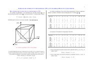
Il existe <strong>des</strong> soli<strong>des</strong> é<strong>la</strong>ncés auxquels on peut raisonnablement appliquer une <strong>des</strong>cription<br />
cinématique et une <strong>des</strong>cription <strong>des</strong> efforts intérieurs plus simples que celles de <strong>la</strong> théorie générale<br />
<strong>des</strong> milieux continus.<br />
x 3<br />
x 2<br />
1<br />
t<br />
p<br />
3<br />
P 3<br />
F<br />
M<br />
x<br />
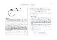
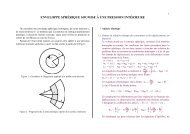
FIGURE: Représentation géométrique d’une poutre rectiligne<br />
Nous traitons dans ce cours du cas <strong>des</strong> <strong>poutres</strong> rectilignes en mouvement p<strong>la</strong>n.<br />
u = u 1 (x 1 , x 3 ) x 1 + u 3 (x 1 , x 3 ) x 3 ∀(x 1 , x 2 , x 3 ) ∈ Ω<br />
Ω = [0, L] × S<br />
Il existe une ligne moyenne C de point courant G, barycentre <strong>des</strong> sections droites S (S⊥C).<br />
MMS 2012, <strong>Introduction</strong> <strong>Introduction</strong> à <strong>la</strong> théorie <strong>des</strong> <strong>poutres</strong> 3/28
Repenser <strong>la</strong> modélisation <strong>des</strong> actions mécaniques<br />
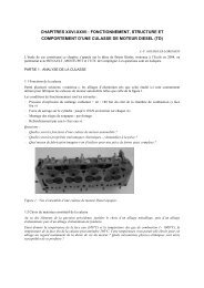
Il ne s’agit plus de considérer les actions transmises par une surface infinitésimale mais celles<br />
transmises par une section droite de <strong>la</strong> poutre.<br />
Ligne moyenne C<br />
σ(x). ~ _ _ x 1<br />
_ x 1<br />
G<br />
_ x 1<br />
S<br />
dS<br />
G<br />
_ x 3<br />
σ(x). ~ _ _ x 1<br />
_ x 1<br />
Ω<br />
-<br />
Ω-<br />
S<br />
FIGURE: Efforts intérieurs transmis par une section droite<br />
Par exemple on s’intéresse à l’effort normal N <strong>des</strong> actions de Ω + sur Ω − (Ω = Ω + ∪ Ω − ) définit<br />
par :<br />
∫<br />
∫<br />
N = σ 11 dS = x 1 · σ ∼ · n dS<br />
S<br />
S<br />
MMS 2012, <strong>Introduction</strong> <strong>Introduction</strong> à <strong>la</strong> théorie <strong>des</strong> <strong>poutres</strong> 4/28
Repenser <strong>la</strong> modélisation <strong>des</strong> actions mécaniques<br />
Travaillons l’équation suivante :<br />
∫<br />
N = x 1 · σ ∼ · n dS<br />
S<br />
MMS 2012, <strong>Introduction</strong> <strong>Introduction</strong> à <strong>la</strong> théorie <strong>des</strong> <strong>poutres</strong> 5/28
Repenser <strong>la</strong> modélisation <strong>des</strong> actions mécaniques<br />
Travaillons l’équation suivante :<br />
∫<br />
N = x 1 · σ ∼ · n dS<br />
S<br />
Prenons un vecteur U ∗ x 1 tel que U,2 ∗ = U∗ ,3 = 0. On a :<br />
∫<br />
∫<br />
N U ∗ = U ∗ x 1 · σ ∼ · n dS = σ ∼ · n · U ∗ x 1 dS<br />
S<br />
S<br />
∀U ∗<br />
Nous allons exploiter le théorème <strong>des</strong> travaux virtuels comme un principe <strong>des</strong> travaux virtuels se<br />
substituant au principe fondamental de <strong>la</strong> statique.<br />
La modélisation <strong>des</strong> efforts de cohésion est déduite du choix d’une <strong>des</strong>cription cinématique<br />
virtuelle x → u ∗ ∀x ∈ Ω.<br />
Nous allons étudier <strong>la</strong> théorie <strong>des</strong> <strong>poutres</strong> de Timoshenko et celle de Navier–Bernoulli (<strong>poutres</strong><br />
minces).<br />
MMS 2012, <strong>Introduction</strong> <strong>Introduction</strong> à <strong>la</strong> théorie <strong>des</strong> <strong>poutres</strong> 5/28
Repenser <strong>la</strong> modélisation <strong>des</strong> actions mécaniques<br />
Les efforts intérieurs peuvent être discontinus du fait d’efforts extérieurs ponctuels (Exemple de<br />
l’effort normal discontinu).<br />
MMS 2012, <strong>Introduction</strong> <strong>Introduction</strong> à <strong>la</strong> théorie <strong>des</strong> <strong>poutres</strong> 6/28
Repenser <strong>la</strong> modélisation <strong>des</strong> actions mécaniques<br />
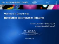
Pour éviter d’utiliser <strong>la</strong> théorie <strong>des</strong> distributions, nous introduisons <strong>la</strong> notion de tronçon de poutre.<br />
Un tronçon est une portion continue de poutre sur <strong>la</strong>quelle les charges extérieures sont continues.<br />
Les discontinuités de chargement et d’appui (condition en dép<strong>la</strong>cement) sont situées aux<br />
l’extrémités <strong>des</strong> tronçons.<br />
x 3<br />
x 2<br />
1<br />
t<br />
p<br />
3<br />
P 3<br />
Tronçon 1<br />
F<br />
M<br />
Tronçon 2<br />
x<br />
FIGURE: Tronçon et discontinuité <strong>des</strong> conditions aux limites<br />
MMS 2012, <strong>Introduction</strong> <strong>Introduction</strong> à <strong>la</strong> théorie <strong>des</strong> <strong>poutres</strong> 6/28
Repenser <strong>la</strong> modélisation <strong>des</strong> actions mécaniques<br />
Pour éviter d’utiliser <strong>la</strong> théorie <strong>des</strong> distributions, nous introduisons <strong>la</strong> notion de tronçon de poutre.<br />
Un tronçon est une portion continue de poutre sur <strong>la</strong>quelle les charges extérieures sont continues.<br />
Les discontinuités de chargement et d’appui (condition en dép<strong>la</strong>cement) sont situées aux<br />
l’extrémités <strong>des</strong> tronçons.<br />
x 3<br />
x 2<br />
1<br />
t<br />
p<br />
3<br />
P 3<br />
Tronçon 1<br />
F<br />
M<br />
Tronçon 2<br />
x<br />
FIGURE: Tronçon et discontinuité <strong>des</strong> conditions aux limites<br />
Les équations d’équilibre portant sur les efforts intérieurs seront écrites tronçon par tronçon.<br />
MMS 2012, <strong>Introduction</strong> <strong>Introduction</strong> à <strong>la</strong> théorie <strong>des</strong> <strong>poutres</strong> 6/28
Application du principe <strong>des</strong> travaux virtuels<br />
La définition d’actions mécaniques et <strong>la</strong> formu<strong>la</strong>tion <strong>des</strong> conditions d’équilibre associées sont<br />
obtenues en mettant en œuvre les étapes suivantes :<br />
Choisir une <strong>des</strong>cription <strong>des</strong> champs virtuels définissant le nouveau modèle mécanique à<br />
partir du modèle 3D usuel (x ∈ Ω → u(x) ∈ H 1 (Ω)).<br />
Calculer les différents travaux virtuels<br />
Appliquer le principe <strong>des</strong> travaux virtuels pour obtenir les équations d’équilibre<br />
Compléter les équations d’équilibre par <strong>des</strong> lois de comportement<br />
Compléter les équations aux dérivées partielles par <strong>des</strong> conditions aux limites<br />
Choisir une géométrie, un matériau et <strong>des</strong> conditions aux limites<br />
Résoudre les équations aux dérivées partielles<br />
Analyser les résultats obtenus<br />
Une autre possibilité est d’appliquer le théorème de l’énergie potentielle pour les systèmes<br />
conservatifs. Le modèle obtenu n’est pas nécessairement le même.<br />
MMS 2012, Application du principe <strong>des</strong> travaux virtuels <strong>Introduction</strong> à <strong>la</strong> théorie <strong>des</strong> <strong>poutres</strong> 7/28
Théorie de Timoshenko<br />
Première étape de <strong>la</strong> mise en œuvre du principe <strong>des</strong> travaux virtuels pour définir les actions<br />
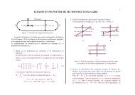
de cohésion : choisir un champ de dép<strong>la</strong>cement virtuel.<br />
*<br />
* *<br />
FIGURE: Description du champ de dép<strong>la</strong>cement virtuel choisi.<br />
u ∗ = u1 ∗ (x 1, x 3 ) x 1 + u3 ∗ (x 1, x 3 ) x 3 ∀(x 1 , x 2 , x 3 ) ∈ Ω (1)<br />
u1 ∗ = U∗ (x 1 ) + θ ∗ (x 1 )x 3 u3 ∗ = V ∗ (x 1 ) (2)<br />
(3)<br />
Il y a trois champs unidimensionnels (U ∗ , V ∗ , θ ∗ ), définis sur l’intervalle [0, L].<br />
MMS 2012, Théorie de Timoshenko <strong>Introduction</strong> à <strong>la</strong> théorie <strong>des</strong> <strong>poutres</strong> 8/28
Théorie de Timoshenko<br />
Première étape de <strong>la</strong> mise en œuvre du principe <strong>des</strong> travaux virtuels pour définir les actions<br />
de cohésion : choisir un champ de dép<strong>la</strong>cement virtuel.<br />
*<br />
* *<br />
FIGURE: Description du champ de dép<strong>la</strong>cement virtuel choisi.<br />
u ∗ = u1 ∗ (x 1, x 3 ) x 1 + u3 ∗ (x 1, x 3 ) x 3 ∀(x 1 , x 2 , x 3 ) ∈ Ω (1)<br />
u1 ∗ = U∗ (x 1 ) + θ ∗ (x 1 )x 3 u3 ∗ = V ∗ (x 1 ) (2)<br />
ε ∗ 11 = U∗ ,1 + θ∗ ,1 x 3 2ε ∗ 13 = V ,1 ∗ + θ∗ (3)<br />
Il y a trois champs unidimensionnels (U ∗ , V ∗ , θ ∗ ), définis sur l’intervalle [0, L].<br />
MMS 2012, Théorie de Timoshenko <strong>Introduction</strong> à <strong>la</strong> théorie <strong>des</strong> <strong>poutres</strong> 8/28
Théorie de Timoshenko<br />
Calcul <strong>des</strong> travaux virtuels.<br />
⋆ Travail virtuel <strong>des</strong> efforts internes<br />
∫<br />
W ∗<br />
int = − ε ∗ ij σ ij dV (4)<br />
Ω<br />
(5)<br />
(6)<br />
MMS 2012, Théorie de Timoshenko <strong>Introduction</strong> à <strong>la</strong> théorie <strong>des</strong> <strong>poutres</strong> 9/28
Théorie de Timoshenko<br />
Calcul <strong>des</strong> travaux virtuels.<br />
⋆ Travail virtuel <strong>des</strong> efforts internes<br />
∫<br />
W ∗<br />
int = − ε ∗ ij σ ij dV (4)<br />
Ω<br />
∫<br />
= − (ε ∗ 11 σ 11 + 2ε ∗ 13 σ 13)dV (5)<br />
Ω<br />
∫<br />
= −<br />
C<br />
( ∫<br />
∫<br />
∫ )<br />
U ∗ ,1 σ 11 dS + θ ∗ ,1 x 3 σ 11 dS + (V ∗ ,1 + θ∗ ) σ 13 dS dx 1 (6)<br />
S<br />
S<br />
S<br />
On introduit alors naturellement les quantités N, T , M conjuguées de U ∗ ,1 , (V ∗ ,1 + θ∗ ), θ ∗ ,1 . Par<br />
définition ce sont l’effort normal, l’effort tranchant et le moment fléchissant (exprimé au point G).<br />
∫<br />
∫<br />
∫<br />
N = σ 11 dS T = σ 13 dS M = x 3 σ 11 dS (7)<br />
S<br />
S<br />
S<br />
Ce sont les composantes du torseur <strong>des</strong> efforts intérieurs. Ceci donne :<br />
∫ (<br />
)<br />
Wint ∗ = − N U,1 ∗ + M θ∗ ,1 + T (V ,1 ∗ + θ∗ ) dx 1 (8)<br />
C<br />
MMS 2012, Théorie de Timoshenko <strong>Introduction</strong> à <strong>la</strong> théorie <strong>des</strong> <strong>poutres</strong> 9/28
Théorie de Timoshenko<br />
Calcul <strong>des</strong> travaux virtuels.<br />
⋆ Travail virtuel <strong>des</strong> efforts internes<br />
⋆ Travail virtuel <strong>des</strong> efforts extérieurs<br />
W ∗ ext = F 0 U ∗ (0) + F L U ∗ (L) + P 0 V ∗ (0) + P L V ∗ (L) + M 0 θ ∗ (0) + M L θ ∗ (L) (9)<br />
∫<br />
(<br />
+ p V ∗ + t U ∗ ) ) dx 1 (10)<br />
C<br />
MMS 2012, Théorie de Timoshenko <strong>Introduction</strong> à <strong>la</strong> théorie <strong>des</strong> <strong>poutres</strong> 10/28
Théorie de Timoshenko, application du principe <strong>des</strong> travaux virtuels<br />
Principe <strong>des</strong> travaux virtuels pour <strong>la</strong> théorie de Timoshenko :<br />
On en déduit les conditions d’équilibre suivantes :<br />
W ∗<br />
int + W ∗ ext = 0 ∀ (U ∗ , V ∗ , θ ∗ ) (11)<br />
N ,1 + t = 0 T ,1 + p = 0 M ,1 − T = 0 (12)<br />
N(0) = −F 0 N(L) = F L T (0) = −P 0 T (L) = P L (13)<br />
M(0) = −M 0 M(L) = M L (14)<br />
MMS 2012, Théorie de Timoshenko <strong>Introduction</strong> à <strong>la</strong> théorie <strong>des</strong> <strong>poutres</strong> 11/28
Théorie de Timoshenko, application du principe <strong>des</strong> travaux virtuels<br />
Démonstration.<br />
W ∗<br />
int + W ∗ ext = 0 ∀ (U ∗ , V ∗ , θ ∗ )<br />
⇓<br />
⎧<br />
⎪⎨<br />
⎪⎩<br />
W ∗<br />
int + W ∗ ext = 0 ∀ U ∗ , avec V ∗ = 0, θ ∗ = 0, U ∗ (0&L) = 0, V ∗ (0&L) = 0, θ ∗ (0&L) = 0<br />
W ∗<br />
int + W ∗ ext = 0 ∀ V ∗ , avec U ∗ = 0, θ ∗ = 0, U ∗ (0&L) = 0, V ∗ (0&L) = 0, θ ∗ (0&L) = 0<br />
W ∗<br />
int + W ∗ ext = 0 ∀ θ ∗ , avec U ∗ = 0, V ∗ = 0, U ∗ (0&L) = 0, V ∗ (0&L) = 0, θ ∗ (0&L) = 0<br />
W ∗<br />
int + W ∗ ext = 0 ∀ (U ∗ , V ∗ , θ ∗ ), avec U ∗ (0) = 0, V ∗ (0&L) = 0, θ ∗ (0&L) = 0<br />
W ∗<br />
int + W ∗ ext = 0 ∀ (U ∗ , V ∗ , θ ∗ ), avec U ∗ (L) = 0, V ∗ (0&L) = 0, θ ∗ (0&L) = 0<br />
W ∗<br />
int + W ∗ ext = 0 ∀ (U ∗ , V ∗ , θ ∗ ), avec U ∗ (0&L) = 0, V ∗ (0) = 0, θ ∗ (0&L) = 0<br />
W ∗<br />
int + W ∗ ext = 0 ∀ (U ∗ , V ∗ , θ ∗ ), avec U ∗ (0&L) = 0, V ∗ (L) = 0, θ ∗ (0&L) = 0<br />
W ∗<br />
int + W ∗ ext = 0 ∀ (U ∗ , V ∗ , θ ∗ ), avec U ∗ (0&L) = 0, V ∗ (0&L) = 0, θ ∗ (0) = 0<br />
W ∗<br />
int + W ∗ ext = 0 ∀ (U ∗ , V ∗ , θ ∗ ), avec U ∗ (0&L) = 0, V ∗ (0&L) = 0, θ ∗ (L) = 0<br />
MMS 2012, Théorie de Timoshenko <strong>Introduction</strong> à <strong>la</strong> théorie <strong>des</strong> <strong>poutres</strong> 12/28
Théorie de Timoshenko, application du principe <strong>des</strong> travaux virtuels<br />
Démonstration.<br />
W ∗<br />
int + W ∗ ext = 0 ∀ (U ∗ , V ∗ , θ ∗ )<br />
⇓<br />
⎧<br />
⎪⎨<br />
⎪⎩<br />
W ∗<br />
int + W ∗ ext = 0 ∀ U ∗ , avec V ∗ = 0, θ ∗ = 0, U ∗ (0&L) = 0, V ∗ (0&L) = 0, θ ∗ (0&L) = 0<br />
W ∗<br />
int + W ∗ ext = 0 ∀ V ∗ , avec U ∗ = 0, θ ∗ = 0, U ∗ (0&L) = 0, V ∗ (0&L) = 0, θ ∗ (0&L) = 0<br />
W ∗<br />
int + W ∗ ext = 0 ∀ θ ∗ , avec U ∗ = 0, V ∗ = 0, U ∗ (0&L) = 0, V ∗ (0&L) = 0, θ ∗ (0&L) = 0<br />
W ∗<br />
int + W ∗ ext = 0 ∀ (U ∗ , V ∗ , θ ∗ ), avec U ∗ (0) = 0, V ∗ (0&L) = 0, θ ∗ (0&L) = 0<br />
W ∗<br />
int + W ∗ ext = 0 ∀ (U ∗ , V ∗ , θ ∗ ), avec U ∗ (L) = 0, V ∗ (0&L) = 0, θ ∗ (0&L) = 0<br />
W ∗<br />
int + W ∗ ext = 0 ∀ (U ∗ , V ∗ , θ ∗ ), avec U ∗ (0&L) = 0, V ∗ (0) = 0, θ ∗ (0&L) = 0<br />
W ∗<br />
int + W ∗ ext = 0 ∀ (U ∗ , V ∗ , θ ∗ ), avec U ∗ (0&L) = 0, V ∗ (L) = 0, θ ∗ (0&L) = 0<br />
W ∗<br />
int + W ∗ ext = 0 ∀ (U ∗ , V ∗ , θ ∗ ), avec U ∗ (0&L) = 0, V ∗ (0&L) = 0, θ ∗ (0) = 0<br />
W ∗<br />
int + W ∗ ext = 0 ∀ (U ∗ , V ∗ , θ ∗ ), avec U ∗ (0&L) = 0, V ∗ (0&L) = 0, θ ∗ (L) = 0<br />
On intègre c<strong>la</strong>ssiquement par parties le travail <strong>des</strong> efforts intérieurs, par exemple :<br />
∫<br />
∫<br />
NU,1 ∗ dx (<br />
1 = (NU ∗ ) ,1 − N ,1 U ∗) ∫<br />
dx 1 = [NU ∗ ] L 0 − N ,1 U ∗ dx 1 (15)<br />
C<br />
C<br />
C<br />
MMS 2012, Théorie de Timoshenko <strong>Introduction</strong> à <strong>la</strong> théorie <strong>des</strong> <strong>poutres</strong> 12/28
Théorie de Timoshenko, application du principe <strong>des</strong> travaux virtuels<br />
Démonstration (suite).<br />
W ∗<br />
int + W ∗ ext = 0 ∀ U ∗ , avec V ∗ = 0, θ ∗ = 0, U ∗ (0&L) = 0, V ∗ (0&L) = 0, θ ∗ (0&L) = 0<br />
∫<br />
∫<br />
⇒ − N U,1 ∗ dx 1 + t U ∗ dx 1 = 0 ∀ U ∗ , avec U ∗ (0) = U ∗ (L) = 0<br />
C<br />
C<br />
∫<br />
∫<br />
⇒ − [NU ∗ ] L 0 + N ,1 U ∗ dx 1 + t U ∗ dx 1 = 0 ∀ U ∗ , avec U ∗ (0) = U ∗ (L) = 0<br />
C<br />
C<br />
⇒ N ,1 + t = 0<br />
∀x 1 ∈ C<br />
MMS 2012, Théorie de Timoshenko <strong>Introduction</strong> à <strong>la</strong> théorie <strong>des</strong> <strong>poutres</strong> 13/28
Théorie de Timoshenko, application du principe <strong>des</strong> travaux virtuels<br />
Démonstration (suite).<br />
W ∗<br />
int + W ∗ ext = 0 ∀ V ∗ , avec U ∗ = 0, θ ∗ = 0, U ∗ (0&L) = 0, V ∗ (0&L) = 0, θ ∗ (0&L) = 0<br />
∫<br />
∫<br />
⇒ − T V,1 ∗ dx 1 + p V ∗ dx 1 = 0 ∀...<br />
C<br />
C<br />
∫<br />
∫<br />
⇒ − [T V ∗ ] L 0 + T ,1 V ∗ dx 1 + p V ∗ dx 1 = 0<br />
C<br />
C<br />
⇒ T ,1 + p = 0<br />
∀x 1 ∈ C<br />
∀...<br />
MMS 2012, Théorie de Timoshenko <strong>Introduction</strong> à <strong>la</strong> théorie <strong>des</strong> <strong>poutres</strong> 14/28
Théorie de Timoshenko, application du principe <strong>des</strong> travaux virtuels<br />
Démonstration (suite).<br />
W ∗<br />
int + W ∗ ext = 0 ∀ θ ∗ , avec U ∗ = 0, V ∗ = 0, U ∗ (0&L) = 0, V ∗ (0&L) = 0, θ ∗ (0&L) = 0<br />
∫<br />
⇒ − M θ,1 ∗ + T θ∗ dx 1 + 0 = 0 ∀...<br />
C<br />
∫<br />
⇒ − [M θ ∗ ] L 0 + M ,1 θ ∗ − T θ ∗ dx 1 + 0 = 0<br />
C<br />
⇒ M ,1 − T = 0<br />
∀...<br />
∀...<br />
MMS 2012, Théorie de Timoshenko <strong>Introduction</strong> à <strong>la</strong> théorie <strong>des</strong> <strong>poutres</strong> 15/28
Cas particulier <strong>des</strong> systèmes isostatiques<br />
Définition : Un système est isostatique si et seulement si on peut déterminer toutes les inconnues<br />
statiques (réactions aux appuis et efforts intérieurs) en utilisant exclusivement les conditions<br />
d’équilibre.<br />
Méthode de résolution <strong>des</strong> systèmes isostatiques :<br />
Identifier quelles sont les inconnues statiques pour chaque liaison,<br />
Rechercher les réactions aux appuis (efforts transmis par les liaisons avec l’extérieur),<br />
Identifier les différents tronçons de <strong>la</strong> poutre,<br />
Considérer l’équilibre de portions de tronçon pour chaque tronçon de <strong>la</strong> poutre,<br />
En déduire N, T, et M,<br />
Utiliser les lois de comportement pour obtenir U ,1 , θ ,1 et V ,1 + θ,<br />
Exploiter les conditions aux limites en dép<strong>la</strong>cement et les conditions de continuité entre les<br />
tronçons, pour obtenir U, V , θ.<br />
MMS 2012, Les systèmes isostatiques <strong>Introduction</strong> à <strong>la</strong> théorie <strong>des</strong> <strong>poutres</strong> 16/28
Cas particulier <strong>des</strong> systèmes isostatiques<br />
Définition : Un système est isostatique si et seulement si on peut déterminer toutes les inconnues<br />
statiques (réactions aux appuis et efforts intérieurs) en utilisant exclusivement les conditions<br />
d’équilibre.<br />
Méthode de résolution <strong>des</strong> systèmes isostatiques :<br />
Identifier quelles sont les inconnues statiques pour chaque liaison,<br />
Rechercher les réactions aux appuis (efforts transmis par les liaisons avec l’extérieur),<br />
Identifier les différents tronçons de <strong>la</strong> poutre,<br />
Considérer l’équilibre de portions de tronçon pour chaque tronçon de <strong>la</strong> poutre,<br />
En déduire N, T, et M,<br />
Utiliser les lois de comportement pour obtenir U ,1 , θ ,1 et V ,1 + θ,<br />
Exploiter les conditions aux limites en dép<strong>la</strong>cement et les conditions de continuité entre les<br />
tronçons, pour obtenir U, V , θ.<br />
Pour les systèmes qui ne sont pas isostatiques, on peut adopter une méthode en dép<strong>la</strong>cement qui<br />
consiste à prendre les dép<strong>la</strong>cements et les rotations comme inconnues principales.<br />
MMS 2012, Les systèmes isostatiques <strong>Introduction</strong> à <strong>la</strong> théorie <strong>des</strong> <strong>poutres</strong> 16/28
Les lois de comportement pour <strong>la</strong> théorie de Timoshenko<br />
On considère un champ de dép<strong>la</strong>cement de <strong>la</strong> forme du champ de dép<strong>la</strong>cement virtuel :<br />
u = u 1 (x 1 , x 3 ) x 1 + u 3 (x 1 , x 3 ) x 3 ∀(x 1 , x 2 , x 3 ) ∈ Ω (16)<br />
u 1 = U(x 1 ) + θ(x 1 )x 3 u 3 = V (x 1 ) (17)<br />
ε 11 = U ,1 + θ ,1 x 3 2ε 13 = V ,1 + θ (18)<br />
Propriété : Les sections droites restent p<strong>la</strong>nes.<br />
Lois de comportement linéaires pour un matériau é<strong>la</strong>stique homogène dans S :<br />
Traction-compression<br />
N = E S U ,1 (19)<br />
∫<br />
Flexion, avec I = x3 2 dS, moment quadratique par rapport à x 2 :<br />
S<br />
M = E I θ ,1 (20)<br />
Cisaillement<br />
T = µ S (θ + V ,1 ) (21)<br />
MMS 2012, Les lois de comportement pour <strong>la</strong> théorie de Timoshenko <strong>Introduction</strong> à <strong>la</strong> théorie <strong>des</strong> <strong>poutres</strong> 17/28
Solution de de Saint-Venant<br />
Sous certaines hypothèses, <strong>la</strong> théorie <strong>des</strong> <strong>poutres</strong> et <strong>la</strong> théorie générale <strong>des</strong> milieux continus<br />
coïncident pour <strong>la</strong> solution de de Saint-Venant.<br />
L’hypothèse de de Saint-Venant consiste à chercher <strong>la</strong> solution du problème d’équilibre d’un<br />
tronçon de poutre droite sous <strong>la</strong> forme d’un état de contrainte contenant uniquement deux<br />
cisaillements et un terme de contrainte axiale :<br />
⎛<br />
( ) σ.. = ⎝ σ ⎞<br />
11 σ 12 σ 13<br />
σ 21 0 0 ⎠ (22)<br />
σ 31 0 0<br />
Les formu<strong>la</strong>tions <strong>des</strong> lois de comportement sont alors liées.<br />
∫ ∫<br />
∫<br />
∫<br />
∫<br />
N = σ 11 dS = Eε 11 dS = Eu 1,1 dS = EU ,1 dS + E(θx 3 ) ,1 dS (23)<br />
S<br />
S<br />
S<br />
S<br />
S<br />
∫<br />
∫<br />
∫<br />
∫<br />
M = x 3 σ 11 dS = x 3 Eε 11 dS = x 3 E U ,1 dS + E x 3 (θx 3 ) ,1 dS (24)<br />
S<br />
S<br />
S<br />
S<br />
∫ ∫<br />
∫<br />
∫<br />
T = σ 13 dS = 2µε 13 dS = µ(u 1,3 + u 3,1 )dS = µ ( )<br />
θ + V ,1 dS (25)<br />
S<br />
S<br />
S<br />
S<br />
MMS 2012, Solution de de Saint-Venant <strong>Introduction</strong> à <strong>la</strong> théorie <strong>des</strong> <strong>poutres</strong> 18/28
Théorème de de Saint-Venant<br />
Loin du point d’application <strong>des</strong> charges, l’influence <strong>des</strong> contraintes sur <strong>la</strong> solution en dép<strong>la</strong>cement<br />
ne dépend que du torseur résultant de <strong>la</strong> distribution <strong>des</strong> contraintes dans les sections droites.<br />
Ainsi, si deux chargements induisent un même troseur d’effort intérieur, alors loin du point<br />
d’application de ces chargements, ils auront <strong>des</strong> conséquences quasiment identiques sur les<br />
déformations.<br />
MMS 2012, Théorème de de Saint-Venant <strong>Introduction</strong> à <strong>la</strong> théorie <strong>des</strong> <strong>poutres</strong> 19/28
Problème aux limites issu de <strong>la</strong> théorie de Timoshenko<br />
Les conditions d’équilibre et les lois de comportement donnent un ensemble d’équations aux<br />
dérivées partielles qu’il faut compléter par <strong>des</strong> conditions aux limites et éventuellement <strong>des</strong><br />
conditions de continuité du dép<strong>la</strong>cement.<br />
Problème de traction, équation d’ordre 2 sur le dép<strong>la</strong>cement longitudinal :<br />
N ,1 + t = 0 N = E S U ,1 ⇒ E S U ,11 + (E S) ,1 U ,1 + t = 0 (26)<br />
Pour avoir une solution unique, il faut 2 conditions aux limites sur U, 1 (N) ou U, pour chaque<br />
tronçon.<br />
Problème de flexion (hypothèse de section constante), équation d’ordre 3 sur les rotations :<br />
T ,1 + p = 0 M ,1 − T = 0 (27)<br />
V ,1 = −θ +<br />
T<br />
µ S M = EIθ ,1 (28)<br />
⇒ E I θ ,111 + p = 0 (29)<br />
Pour obtenir une solution unique en θ, il faut 3 conditions aux limites sur θ, θ ,1 ou θ ,11 , pour<br />
chaque tronçon. La continuité du dép<strong>la</strong>cement impose <strong>la</strong> continuité de θ et de V .<br />
MMS 2012, Problème aux limites <strong>Introduction</strong> à <strong>la</strong> théorie <strong>des</strong> <strong>poutres</strong> 20/28
Expression <strong>des</strong> contraintes locales<br />
Connaissant x 1 → (U, V , θ) ∀ x 1 ∈ [0, L], il est possible de calculer ε ∼<br />
(u) et d’en déduire σ ∼<br />
en<br />
utilisant <strong>la</strong> loi de comportement de <strong>la</strong> théorie générale <strong>des</strong> milieux continus.<br />
⎛<br />
( ) ⎜<br />
U ,1 + θ ,1 x 3 0<br />
ε.. = ⎝<br />
V ,1 +θ<br />
2<br />
0 0 0<br />
V ,1 +θ<br />
2 0 0<br />
⎞<br />
⎟<br />
⎠ (30)<br />
On obtient en particulier :<br />
σ 11 = E (U ,1 + θ ,1 x 3 )<br />
⇒ σ 11 = N S + M I<br />
x 3<br />
Le maximum de contrainte est obtenu au point le plus éloigné en x 3 de <strong>la</strong> ligne moyenne. Ce point<br />
a pour coordonnée x 3 = ρ :<br />
max<br />
(x 2 , x 3 )∈S σ 11 = N S + M I<br />
ρ<br />
MMS 2012, Contraintes locales <strong>Introduction</strong> à <strong>la</strong> théorie <strong>des</strong> <strong>poutres</strong> 21/28
Théorie de Navier-Bernoulli<br />
Dans <strong>la</strong> théorie qui a été développée jusque là, une section p<strong>la</strong>ne reste p<strong>la</strong>ne, mais pas<br />
perpendicu<strong>la</strong>ire à l’axe neutre. Si les cisaillements sont faibles (effet du moment dominant), il est<br />
raisonnable de rajouter cette dernière hypothèse à l’aide d’une liaison interne. On retrouve alors <strong>la</strong><br />
théorie dite c<strong>la</strong>ssiquement de Navier-Bernoulli.<br />
*<br />
* *<br />
FIGURE: Description du champ de dép<strong>la</strong>cement virtuel choisi.<br />
u ∗ = u1 ∗ (x 1, x 3 ) x 1 + u3 ∗ (x 1, x 3 ) x 3 ∀(x 1 , x 2 , x 3 ) ∈ Ω (31)<br />
u1 ∗ = U∗ (x 1 ) + θ ∗ (x 1 )x 3 u 3 = V ∗ (x 1 ) V,1 ∗ + θ∗ = 0 (32)<br />
ε ∗ 11 = U∗ ,1 + θ∗ ,1 x 3 2ε ∗ 13 = 0 (33)<br />
Il y a deux champs unidimensionnels indépendants (U ∗ , V ∗ ), définis sur l’intervalle [0, L].<br />
MMS 2012, Théorie de Navier-Bernoulli <strong>Introduction</strong> à <strong>la</strong> théorie <strong>des</strong> <strong>poutres</strong> 22/28
Théorie de Navier-Bernoulli<br />
Problème de traction, équation d’ordre 2 sur le dép<strong>la</strong>cement longitudinal :<br />
N ,1 + t = 0 N = E S U ,1 ⇒ E S U ,11 + (E S) ,1 U ,1 + t = 0 (34)<br />
Pour avoir une solution unique, il faut 2 conditions aux limites sur U, 1 (N) ou U, pour chaque<br />
tronçon.<br />
Problème de flexion (hypothèse de section constante), équation d’ordre 4 sur le dép<strong>la</strong>cement<br />
transverse :<br />
M ,11 + p = 0 T = M ,1 (35)<br />
M = −E I V ,11 (36)<br />
⇒ E I V ,1111 = p (37)<br />
Pour obtenir une solution unique il faut 4 conditions aux limites sur V , V ,1 , V ,11 ou V ,111 , pour<br />
chaque tronçon. La continuité du dép<strong>la</strong>cement impose <strong>la</strong> continuité de θ = −V ,1 et de V .<br />
Pour établir les conditions d’équilibre, il faut tenir compte de l’indépendance <strong>des</strong> fonctions V ,1 et V .<br />
MMS 2012, Théorie de Navier-Bernoulli <strong>Introduction</strong> à <strong>la</strong> théorie <strong>des</strong> <strong>poutres</strong> 23/28
Théorie de Navier-Bernoulli, exemple d’une poutre encastrée soumise<br />
à son poids propre<br />
¢¡¢<br />
x 1<br />
¢¡¢<br />
¢¡¢<br />
¥¤¥¤¥¤¥¤¥¤¥¤¥¤¥¤¥¤¥¤¥¤¥¤¥¤¥¤¥¤¥¤¥¤¥¤¥¤¥¤¥¤¥¤¥¤¥¤¥¤¥¤¥¤¥¤¥¤¥¤¥¤¥¤¥¤¥¤¥¤¥¤¥¤¥¤¥¤¥¤¥¤¥¤¥¤¥¤¥¤¥¤¥¤¥¤¥¤¥¤¥¤¥¤¥¤¥¤¥¤¥¤¥¤¥¤¥¤¥¤¥¤¥<br />
£¤£¤£¤£¤£¤£¤£¤£¤£¤£¤£¤£¤£¤£¤£¤£¤£¤£¤£¤£¤£¤£¤£¤£¤£¤£¤£¤£¤£¤£¤£¤£¤£¤£¤£¤£¤£¤£¤£¤£¤£¤£¤£¤£¤£¤£¤£¤£¤£¤£¤£¤£¤£¤£¤£¤£¤£¤£¤£¤£¤£¤£<br />
¢¡¢<br />
¥¤¥¤¥¤¥¤¥¤¥¤¥¤¥¤¥¤¥¤¥¤¥¤¥¤¥¤¥¤¥¤¥¤¥¤¥¤¥¤¥¤¥¤¥¤¥¤¥¤¥¤¥¤¥¤¥¤¥¤¥¤¥¤¥¤¥¤¥¤¥¤¥¤¥¤¥¤¥¤¥¤¥¤¥¤¥¤¥¤¥¤¥¤¥¤¥¤¥¤¥¤¥¤¥¤¥¤¥¤¥¤¥¤¥¤¥¤¥¤¥¤¥<br />
£¤£¤£¤£¤£¤£¤£¤£¤£¤£¤£¤£¤£¤£¤£¤£¤£¤£¤£¤£¤£¤£¤£¤£¤£¤£¤£¤£¤£¤£¤£¤£¤£¤£¤£¤£¤£¤£¤£¤£¤£¤£¤£¤£¤£¤£¤£¤£¤£¤£¤£¤£¤£¤£¤£¤£¤£¤£¤£¤£¤£¤£<br />
¥¤¥¤¥¤¥¤¥¤¥¤¥¤¥¤¥¤¥¤¥¤¥¤¥¤¥¤¥¤¥¤¥¤¥¤¥¤¥¤¥¤¥¤¥¤¥¤¥¤¥¤¥¤¥¤¥¤¥¤¥¤¥¤¥¤¥¤¥¤¥¤¥¤¥¤¥¤¥¤¥¤¥¤¥¤¥¤¥¤¥¤¥¤¥¤¥¤¥¤¥¤¥¤¥¤¥¤¥¤¥¤¥¤¥¤¥¤¥¤¥¤¥<br />
£¤£¤£¤£¤£¤£¤£¤£¤£¤£¤£¤£¤£¤£¤£¤£¤£¤£¤£¤£¤£¤£¤£¤£¤£¤£¤£¤£¤£¤£¤£¤£¤£¤£¤£¤£¤£¤£¤£¤£¤£¤£¤£¤£¤£¤£¤£¤£¤£¤£¤£¤£¤£¤£¤£¤£¤£¤£¤£¤£¤£¤£<br />
¢¡¢<br />
¥¤¥¤¥¤¥¤¥¤¥¤¥¤¥¤¥¤¥¤¥¤¥¤¥¤¥¤¥¤¥¤¥¤¥¤¥¤¥¤¥¤¥¤¥¤¥¤¥¤¥¤¥¤¥¤¥¤¥¤¥¤¥¤¥¤¥¤¥¤¥¤¥¤¥¤¥¤¥¤¥¤¥¤¥¤¥¤¥¤¥¤¥¤¥¤¥¤¥¤¥¤¥¤¥¤¥¤¥¤¥¤¥¤¥¤¥¤¥¤¥¤¥<br />
£¤£¤£¤£¤£¤£¤£¤£¤£¤£¤£¤£¤£¤£¤£¤£¤£¤£¤£¤£¤£¤£¤£¤£¤£¤£¤£¤£¤£¤£¤£¤£¤£¤£¤£¤£¤£¤£¤£¤£¤£¤£¤£¤£¤£¤£¤£¤£¤£¤£¤£¤£¤£¤£¤£¤£¤£¤£¤£¤£¤£¤£<br />
x 3<br />
¢¡¢<br />
¢¡¢<br />
¢¡¢<br />
¡<br />
0<br />
¥¤¥¤¥¤¥¤¥¤¥¤¥¤¥¤¥¤¥¤¥¤¥¤¥¤¥¤¥¤¥¤¥¤¥¤¥¤¥¤¥¤¥¤¥¤¥¤¥¤¥¤¥¤¥¤¥¤¥¤¥¤¥¤¥¤¥¤¥¤¥¤¥¤¥¤¥¤¥¤¥¤¥¤¥¤¥¤¥¤¥¤¥¤¥¤¥¤¥¤¥¤¥¤¥¤¥¤¥¤¥¤¥¤¥¤¥¤¥¤¥¤¥<br />
£¤£¤£¤£¤£¤£¤£¤£¤£¤£¤£¤£¤£¤£¤£¤£¤£¤£¤£¤£¤£¤£¤£¤£¤£¤£¤£¤£¤£¤£¤£¤£¤£¤£¤£¤£¤£¤£¤£¤£¤£¤£¤£¤£¤£¤£¤£¤£¤£¤£¤£¤£¤£¤£¤£¤£¤£¤£¤£¤£¤£¤£<br />
L<br />
¥¤¥¤¥¤¥¤¥¤¥¤¥¤¥¤¥¤¥¤¥¤¥¤¥¤¥¤¥¤¥¤¥¤¥¤¥¤¥¤¥¤¥¤¥¤¥¤¥¤¥¤¥¤¥¤¥¤¥¤¥¤¥¤¥¤¥¤¥¤¥¤¥¤¥¤¥¤¥¤¥¤¥¤¥¤¥¤¥¤¥¤¥¤¥¤¥¤¥¤¥¤¥¤¥¤¥¤¥¤¥¤¥¤¥¤¥¤¥¤¥¤¥<br />
£¤£¤£¤£¤£¤£¤£¤£¤£¤£¤£¤£¤£¤£¤£¤£¤£¤£¤£¤£¤£¤£¤£¤£¤£¤£¤£¤£¤£¤£¤£¤£¤£¤£¤£¤£¤£¤£¤£¤£¤£¤£¤£¤£¤£¤£¤£¤£¤£¤£¤£¤£¤£¤£¤£¤£¤£¤£¤£¤£¤£¤£<br />
¡<br />
¥¤¥¤¥¤¥¤¥¤¥¤¥¤¥¤¥¤¥¤¥¤¥¤¥¤¥¤¥¤¥¤¥¤¥¤¥¤¥¤¥¤¥¤¥¤¥¤¥¤¥¤¥¤¥¤¥¤¥¤¥¤¥¤¥¤¥¤¥¤¥¤¥¤¥¤¥¤¥¤¥¤¥¤¥¤¥¤¥¤¥¤¥¤¥¤¥¤¥¤¥¤¥¤¥¤¥¤¥¤¥¤¥¤¥¤¥¤¥¤¥¤¥<br />
£¤£¤£¤£¤£¤£¤£¤£¤£¤£¤£¤£¤£¤£¤£¤£¤£¤£¤£¤£¤£¤£¤£¤£¤£¤£¤£¤£¤£¤£¤£¤£¤£¤£¤£¤£¤£¤£¤£¤£¤£¤£¤£¤£¤£¤£¤£¤£¤£¤£¤£¤£¤£¤£¤£¤£¤£¤£¤£¤£¤£¤£<br />
¢¡¢<br />
FIGURE: Poutre encastrée, p = −ρ S g, U(0) = V (0) = 0, θ(0) = 0, N(L) = 0, M(L) = 0, T (L) = M ,1 (L) = 0.<br />
Il n’y a qu’un seul tronçon.<br />
Problème de traction :<br />
E S U ,11 = 0 U(0) = 0 U ,1 (L) = 0 (38)<br />
Problème de flexion :<br />
E I V ,1111 = p V (0) = 0 V ,1 (0) = 0 V ,11 (L) = 0 V ,111 (L) = 0 (39)<br />
MMS 2012, Théorie de Navier-Bernoulli <strong>Introduction</strong> à <strong>la</strong> théorie <strong>des</strong> <strong>poutres</strong> 24/28
Théorie de Navier-Bernoulli, exemple d’une poutre encastrée soumise<br />
à son poids propre<br />
Solution :<br />
Flèche de <strong>la</strong> poutre :<br />
V =<br />
U = 0 ∀x 1<br />
p<br />
2 E I ( x 4 1<br />
12 − L 3 x 3 1 + L2<br />
2 x 2 1 )<br />
V (L) =<br />
p<br />
8 E I L4<br />
MMS 2012, Théorie de Navier-Bernoulli <strong>Introduction</strong> à <strong>la</strong> théorie <strong>des</strong> <strong>poutres</strong> 25/28
Théorie de Navier-Bernoulli, approche par le théorème de l’énergie<br />
potentielle<br />
Nous introduisons l’énergie potentielle qui sera exploitée dans le cours sur <strong>la</strong> théorie <strong>des</strong><br />
bifurcations et pour celui sur <strong>la</strong> théorie de stabilité.<br />
Il possible de déduire les lois de comportement <strong>des</strong> re<strong>la</strong>tions issues de <strong>la</strong> théorie générale <strong>des</strong><br />
milieux continus en appliquant le théorème de l’énergie potentielle avec l’hypothèse cinématique<br />
de Navier-Bernoulli.<br />
u = u 1 (x 1 , x 3 ) x 1 + u 3 (x 1 , x 3 ) x 3 ∀(x 1 , x 2 , x 3 ) ∈ Ω (40)<br />
u 1 = U(x 1 ) + θ(x 1 )x 3 u 3 = V (x 1 ) V ,1 + θ = 0 (41)<br />
⎛<br />
( ) ε.. = ⎝ U ⎞<br />
,1 − V ,11 x 3 0 0<br />
0 0 0⎠ (42)<br />
0 0 0<br />
W (ε ∼<br />
) = E 2 ε2 11<br />
∫ ∫<br />
F(U, V ) = W (ε ∼<br />
) dS dx 1 (43)<br />
C S<br />
− F 0 U(0) − F L U(L) − P 0 V (0) − P L V (L) − M 0 θ(0) − M L θ(L) (44)<br />
∫<br />
− (p V + t U) dx 1 (45)<br />
C<br />
MMS 2012, Théorie de Navier-Bernoulli <strong>Introduction</strong> à <strong>la</strong> théorie <strong>des</strong> <strong>poutres</strong> 26/28
Théorie de Navier-Bernoulli, approche par le théorème de l’énergie<br />
potentielle<br />
Pour éliminer les mouvements de corps rigide on considère une poutre encastrée en x 1 = 0 :<br />
δV (0) = 0 et δV ,1 (0).<br />
∫ ∫<br />
F ,V (U, V )[δV ] = W ′ (ε ∼<br />
) : ∼<br />
ε,V [δV ] dS dx 1 (46)<br />
C S<br />
− P 0 δV (0) − P L δV (L) − M 0 δθ(0) − M L δθ(L) (47)<br />
∫<br />
− p δV dx 1 (48)<br />
C<br />
avec :<br />
⎛<br />
( ε,V [δV ] ) = ⎝ −δV ⎞<br />
,11x 3 0 0<br />
0 0 0⎠ (49)<br />
0 0 0<br />
donc (hypothèse de section constante) :<br />
∫ ∫<br />
∫<br />
W ′ (ε ∼<br />
) : ∼<br />
ε,V [δV ] dS dx 1 = E I V ,11 δV ,11 dx 1 (50)<br />
C S<br />
C<br />
= [ ∫<br />
] L<br />
E I V ,11 δV ,1 0 − E I V ,111 δV ,1 dx 1 (51)<br />
C<br />
= − [ E I V ,11 δθ ] L<br />
0 − [ E I V ,111 δV ] ∫<br />
L<br />
0 + E I V ,1111 δV dx 1<br />
C<br />
(52)<br />
MMS 2012, Théorie de Navier-Bernoulli <strong>Introduction</strong> à <strong>la</strong> théorie <strong>des</strong> <strong>poutres</strong> 27/28
Théorie de Navier-Bernoulli, approche par le théorème de l’énergie<br />
potentielle<br />
F ,V (U, V )[δV ] = − [ E I V ,11 δθ ] L<br />
0 − [ E I V ,111 δV ] L<br />
(53)<br />
0<br />
∫<br />
+ E I V ,1111 δV dx 1 (54)<br />
C<br />
− P 0 δV (0) − P L δV (L) − M 0 δθ(0) − M L δθ(L) (55)<br />
∫<br />
− p δV dx 1 (56)<br />
C<br />
Application du théorème de l’énergie potentielle :<br />
F ,U (U, V )[δU] = 0<br />
∀ δU<br />
F ,V (U, V )[δV ] = 0<br />
On retrouve les équations obtenues avec le principe <strong>des</strong> travaux virtuels en prenant δU = U ∗ et<br />
δV = V ∗ .<br />
∀ δV<br />
MMS 2012, Théorie de Navier-Bernoulli <strong>Introduction</strong> à <strong>la</strong> théorie <strong>des</strong> <strong>poutres</strong> 28/28