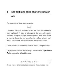
1 Modelli per serie storiche univariate

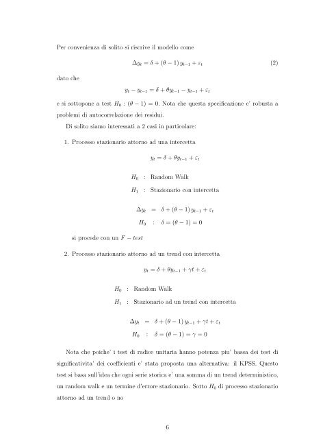
Per convenienza di solito si riscrive il modello come
dato che
∆yt = δ + (θ − 1) yt−1 + εt
yt − yt−1 = δ + θyt−1 − yt−1 + εt
e si sottopone a test H0 : (θ − 1) = 0. Nota che questa specificazione e’ robusta a
problemi di autocorrelazione dei residui.
Di solito siamo interessati a 2 casi in particolare:
1. Processo stazionario attorno ad una intercetta
si procede con un F − test
yt = δ + θyt−1 + εt
H0 : Random Walk
H1 : Stazionario con intercetta
∆yt = δ + (θ − 1) yt−1 + εt
H0 : δ = (θ − 1) = 0
2. Processo stazionario attorno ad un trend con intercetta
H0 : Random Walk
yt = δ + θyt−1 + γt + εt
H1 : Stazionario ad un trend con intercetta
∆yt = δ + (θ − 1) yt−1 + γt + εt
H0 : δ = (θ − 1) = γ = 0
Nota che poiche’ i test di radice unitaria hanno potenza piu’ bassa dei test di
significativita’ dei coefficienti e’ stata proposta una alternativa: il KPSS. Questo
test si basa sull’idea che ogni serie storica e’ una somma di un trend deterministico,
un random walk e un termine d’errore stazionario. Sotto H0 di processo stazionario
attorno ad un trend o no
6
(2)