Il dominio della frequenza
Il dominio della frequenza
Il dominio della frequenza

You also want an ePaper? Increase the reach of your titles
YUMPU automatically turns print PDFs into web optimized ePapers that Google loves.
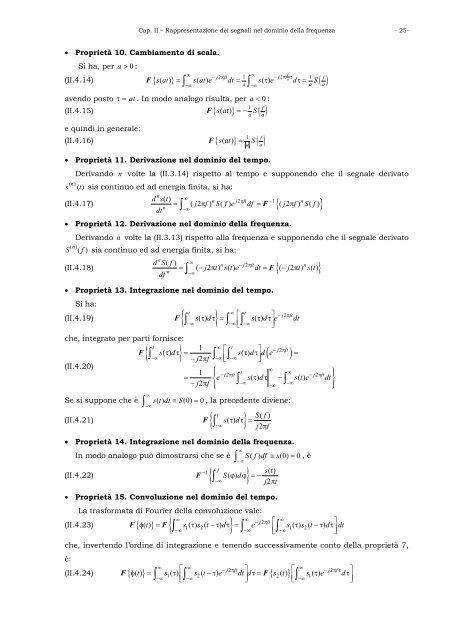
Cap. II – Rappresentazione dei segnali nel <strong>dominio</strong> <strong>della</strong> <strong>frequenza</strong> - 25-<br />
• Proprietà 10. Cambiamento di scala.<br />
Si ha, per a > 0 :<br />
(II.4.14) F { sat 2<br />
2<br />
( )} ∞ sate ( ) 1 f<br />
− j πft j a<br />
( )<br />
1 f<br />
=<br />
∫<br />
dt = ∞ s e − π τ d S<br />
a∫<br />
τ τ = a<br />
(<br />
a<br />
)<br />
avendo posto τ= at . In modo analogo risulta, per a < 0 :<br />
1 f<br />
(II.4.15) F { sat ( )} =− S ( )<br />
e quindi in generale:<br />
1 f<br />
(II.4.16) F { sat ( )} = S ( )<br />
• Proprietà 11. Derivazione nel <strong>dominio</strong> del tempo.<br />
s (n) (t)<br />
−∞<br />
Derivando n volte la (II.3.14) rispetto al tempo e supponendo che il segnale derivato<br />
sia continuo ed ad energia finita, si ha:<br />
n<br />
d s()<br />
t ∞<br />
n j<br />
(II.4.17) ( 2 ) ( ) 2 πft − 1 n<br />
= j π f S f e df = {( j2 πf) S( f)<br />
}<br />
dt<br />
n<br />
−∞<br />
a<br />
a<br />
−∞<br />
∫ F<br />
• Proprietà 12. Derivazione nel <strong>dominio</strong> <strong>della</strong> <strong>frequenza</strong>.<br />
Derivando n volte la (II.3.13) rispetto alla <strong>frequenza</strong> e supponendo che il segnale derivato<br />
S (n) ( f )<br />
sia continuo ed ad energia finita, si ha:<br />
n<br />
d S( f)<br />
∞<br />
n −j (II.4.18) ( 2 ) ( ) 2 πft n<br />
= −j π t s t e dt = {( −j2 πt) s( t)<br />
}<br />
df<br />
n<br />
∫<br />
F<br />
• Proprietà 13. Integrazione nel <strong>dominio</strong> del tempo.<br />
Si ha:<br />
j2<br />
(II.4.19) F { s() τ dτ } = s()<br />
τ dτ<br />
e<br />
che, integrato per parti fornisce:<br />
(II.4.20)<br />
Se si suppone che è<br />
F<br />
−∞<br />
t<br />
∞<br />
⎡<br />
⎢⎣<br />
∫ ∫ ∫<br />
−∞ −∞ −∞<br />
t<br />
a<br />
a<br />
⎤<br />
⎥⎦<br />
−<br />
πft<br />
t<br />
{ } () 1 ∞ t<br />
()<br />
j2<br />
ft<br />
s d<br />
⎡<br />
s d<br />
⎤ − π<br />
∫ d( e )<br />
−∞ ∫−∞ ⎢∫−∞<br />
⎥<br />
∫<br />
∞<br />
−∞<br />
τ τ = τ τ =<br />
−j2πf<br />
⎣ ⎦<br />
1 ⎧<br />
2<br />
t<br />
∞<br />
⎪ j ft<br />
∞<br />
⎫<br />
− π −j2πft<br />
⎪<br />
= ⎨e s() τ dτ − s()<br />
t e dt⎬<br />
−j2πf<br />
∫−∞<br />
∫<br />
−∞<br />
−∞<br />
⎩⎪ ⎭⎪<br />
stdt () ≡ S(0) = 0, la precedente diviene:<br />
t S( f)<br />
(II.4.21) F { s()<br />
d }<br />
∫ τ τ = −∞ j2πf<br />
• Proprietà 14. Integrazione nel <strong>dominio</strong> <strong>della</strong> <strong>frequenza</strong>.<br />
In modo analogo può dimostrarsi che se è S( f) df ≡ s(0) = 0, è<br />
−<br />
f<br />
(II.4.22) F { ∫<br />
S( ) d<br />
−∞<br />
}<br />
∫<br />
∞<br />
−∞<br />
1 s()<br />
t<br />
ϕ ϕ =−<br />
j2πt<br />
• Proprietà 15. Convoluzione nel <strong>dominio</strong> del tempo.<br />
La trasformata di Fourier <strong>della</strong> convoluzione vale:<br />
ft<br />
() t ∞ s1() s2( t ) d ∞ − π<br />
φ = e<br />
⎡<br />
∞<br />
s1() s2( t ) d<br />
⎤<br />
∫<br />
τ −τ τ = dt<br />
−∞ ∫<br />
τ −τ τ<br />
−∞ ⎢⎣<br />
∫−∞<br />
⎥⎦<br />
j2<br />
(II.4.23) F{ } F { }<br />
che, invertendo l’ordine di integrazione e tenendo successivamente conto <strong>della</strong> proprietà 7,<br />
è:<br />
j<br />
(II.4.24) { } 2 ft j<br />
{ }<br />
2 f<br />
() t ∞ s1() ∞ − π<br />
s2( t ) e dt d s2() t ∞ − π τ<br />
F φ =<br />
⎡ ⎤ ⎡<br />
∫<br />
τ −τ τ= s1()<br />
τ e dτ<br />
−∞ ⎢⎣∫−∞ ⎥<br />
F<br />
⎤<br />
⎦ ⎢⎣∫−∞<br />
⎥⎦<br />
dt