i AN ASSESSMENT OF TOMATO PRICE VARIABILITY IN LUSAKA ...

AN ASSESSMENT OF TOMATO PRICE VARIABILITY IN LUSAKA AND ITS 

EFFECTS ON SMALLHOLDER FARMERS 

By 

Mukwiti Nchooli Mwiinga 

THESIS 

Submitted to 

Michigan State University 

in partial fulfillment of the requirements 

for the degree of 

MASTERS OF SCIENCE 

Agricultural, Food and Resource Economics 

2009 

i

ABSTRACT 

AN ASSESSMENT OF TOMATO PRICE VARIABILITY IN LUSAKA AND ITS 

EFFECTS ON SMALLHOLDER FARMERS 

By 

Mukwiti Nchooli Mwiinga 

This paper discusses the structure and operation of the tomato subsector in Lusaka 

(Zambia), establishes the level of price variability for tomatoes in Lusaka’s Soweto 

market, and assesses the impact of tomato price variability on returns to tomato 

production. Price variability determination involved analysis of the coefficient of 

variation, conditional variance and the ratio of the mean absolute positive to negative 

price prediction errors. These results were compared with four other wholesale markets in 

Costa Rica, Taiwan, Sri Lanka, and the United States of America (Chicago). These other 

countries were chosen to capture a wide range of supply chain development, as proxied 

by purchasing power parity Gross Domestic Product (PPP GDP). The study revealed that 

(a) PPP GDP is strongly negatively (positively) associated with price variability 

(predictability), and (b) Zambia has the lowest PPP GDP, highest price variability, and 

least tomato price predictability. Monte Carlo simulation analysis was then conducted to 

establish the effect that three different scenarios would have on the tomato farmers’ net 

returns. Increased sales frequency reduces the variability of expected price but has no 

recognizable impact on the variability of profits. Supply chain improvements also 

reduced the variability of prices. The production of high quality tomatoes has very 

significant effects on returns to farmers. Some policy implications drawn include, the 

need to establish formal grades and standards, investment in cold chain systems and 

general improvement in the traditional wholesale and retail market infrastructure. 

ii

DEDICATION 

This thesis is dedicated to my family: my late father, Elijah Musembwa Mwiinga, my 

mother, Margaret Duntuula Mwiinga, my siblings Malita, Maelo, Mugwagwa and 

Mutinta, and my nieces Chiedza and Duntuula. Special dedication goes to my dearest 

father who always insisted on hard work and discipline in school, and to my mother for 

all her love and support during my studies, but most importantly, for being the 

‘superwoman’ in my life. 

iii

ACKNOWLEDGEMENT 

I would like to express my sincere thanks and appreciation to all those who helped me 

finish my degree at Michigan State University (MSU). I am especially grateful to my 

major professor, Dr. David Tschirley, for his support throughout my masters program. 

His guidance, encouragement and understanding provided an ideal atmosphere for the 

timely and proper completion of this work. My thanks also go to the other two members 

of my thesis committee - Dr. Hamish Gow from the Department of Agricultural and 

Resource Economics and Dr. Randy Beaudry from the Department of Horticulture, for 

their valuable comments and suggestions. I am also thankful to Dr. Cynthia Donovan for 

her assistance in selecting the courses I took during my masters program and her 

preliminary ideas on my thesis. 

Special thanks go to the USAID Initiative for Long-term Training and Capacity Building 

Program (UILTCB) administered through the Bean/Cowpea Creative Research Support 

Project (CRSP) at MSU for the financial support throughout my masters program. From 

the Bean Cowpea CRSP, I am thankful to Dr. Irvin Widders, Dr. Mywish Maredia and 

Mr. Ben Hassankhani for the important administrative role they played prior to and 

during my masters program. 

I am also thankful to the University of Zambia, School of Agricultural Sciences for 

nominating me to participate on the UILTCB program and the Staff Development Office 

for their fellowship support during the research phase of my program. Special thanks go 

iv

to the Dean, School of Agricultural Science, Dr. Judith Lungu, and Dr. Olusegun 

Yerokun for their leadership, facilitation and support throughout my studies. 

My Sincere thanks also go to the Food Security Research Project (FSRP, Zambia) which 

matched my research funds for the successful administering and completion of my 

tomato survey, and also provided me with additional data for my research (tomato price 

collection data and urban survey consumption data) and research support; field and office 

resources and facilities. I am greatly indebted to Dr. Mike Weber who had his office 

partitioned to create office space for me. I am also thankful to all the other FSRP staff 

for the various ways in which they were of assistance to me, with special thanks going to 

Mr. Munguzwe Hichaambwa, Mr. Kennedy Malambo and Esnart Musukwa, who I 

closely worked with during my survey and data analysis. 

I’d like to also thank all the other faculty in the Department Of Agricultural, and Food 

Resource Economics at MSU for their contribution to my professional development 

during my stay at MSU; my classmates and friends who made my stay at MSU happier 

and memorable - I am specially thankful to Lillian and Sindi Kirimi and their two 

daughters, Eric Bailey, Alda Tomo and Keneilwe Kgosikoma; and my fellow UILTCB 

candidates who were like my family away from home, especially Mwape Malunga, 

Dingiswayo Banda and Patrick Ofori. 

Last but not the least, I am thankful to my God and Savior, Jesus Christ, for the blessings 

he continues to bestow on my life. 

v

TABLE OF CONTENTS 

LIST OF TABLES ........................................................................................................... ix 

LIST OF FIGURES ......................................................................................................... xi 

KEY TO ABBREVIATIONS......................................................................................... xii 

CHAPTER 1 .......................................................................................................................1 

INTRODUCTION..............................................................................................................1 

1.1 Background ........................................................................................................1 

1.1.1 The Situation in Zambia ............................................................................4 

1.2 Objectives of the Study .....................................................................................7 

1.3 Organization of Thesis .......................................................................................8 

CHAPTER TWO .............................................................................................................10 

TOMATO PRODUCTION AND MARKETING SYSTEM SERVING LUSAKA ..10 

2.1 Data ...................................................................................................................10 

2.1.1 Urban Consumption Survey Data ..........................................................10 

2.1.2 Tomato Wholesale and Retail Price and Quantity Data .....................11 

2.1.3 Data on Procurement Systems ................................................................12 

2.2 Methods .............................................................................................................13 

2.3 Fresh Produce in Consumer Budget Shares ..................................................15 

2.4 The Structure of the Tomato Production and Marketing System Serving 

Lusaka ...........................................................................................................................19 

2.4.1 Overview ...................................................................................................20 

2.4.2 The “Traditional” Sector ........................................................................22 

2.4.3 The ‘Modern’ Sector: Supermarkets and Processors ..........................33 

2.5 Price Behavior ..................................................................................................40 

2.5.1 Weekly Wholesale Prices in Soweto Market .........................................40 

2.5.2 Weighted Average Prices by Marketing Channel ................................41 

2.5.3 Tomato Wholesale and Retail Prices......................................................42 

2.5 Summary and Conclusions..............................................................................47 

2.5.1 Importance of Tomatoes..........................................................................47 

2.5.2 The Tomato Subsector .............................................................................47 

CHAPTER 3 .....................................................................................................................51 

TOMATO PRICE VARIABILITY AT WHOLESALE LEVEL: COMPARING 

SOWETO MARKET (ZAMBIA) WITH OTHER WHOLESALE MARKETS 

ACROSS THE WORLD .................................................................................................51 

3.1 Factors Influencing Price Variability and Predictability .............................51 

3.2 Hypothesis Testing ...........................................................................................59 

3.3 Data and Methods ............................................................................................60 

3.3.1 Data ...........................................................................................................60 

3.3.2 Methods .....................................................................................................62 

3.4 Results ...............................................................................................................65 

vi

3.4.1 Variability and Predictability of Prices .................................................65 

3.4.2 The Problem of Predicting Sharp Price Declines ..................................69 

3.5 Summary and Discussion ................................................................................71 

3.5.1 Tomato Seasonality of Supply.................................................................75 

3.5.2 Tomato Supply Shocks ............................................................................78 

3.5.3 Random Fluctuations in the Quantities of Tomatoes Arriving in the 

Market 79 

CHAPTER 4 .....................................................................................................................82 

MONTE CARLO ANALYSIS OF CONDITIONAL AND UNCONDITIONAL NET 

RETURNS TO TOMATO PRODUCTION ..................................................................82 

4.1 Household Survey ............................................................................................84 

4.2 Price Data .........................................................................................................86 

4.3 Overview of Monte Carlo Analysis ................................................................87 

4.4 The Monte Carlo Model ..................................................................................89 

4.5 Results .............................................................................................................102 

4.5.1 Distributions of Farmer Profits ............................................................102 

4.5.2 Simulation Results for the Different Scenarios ...................................103 

4.6 Chapter Summary and Conclusion ..............................................................113 

CHAPTER 5 ...................................................................................................................117 

CONCLUSION ..............................................................................................................117 

5.1 Summary of key results .................................................................................118 

5.1.1 Importance of Tomatoes........................................................................118 

5.1.2 The Tomato Subsector ...........................................................................118 

5.1.3 Tomato Price Variability and Predictability .......................................122 

5.1.4 Baseline and Different Scenarios on Net Returns to Tomato 

Production ..............................................................................................................125 

5.2 Contributions and Limitations of the Study ................................................127 

5.3 Future Research .............................................................................................130 

5.4 Policy Implications and Recommendations .................................................131 

APPENDICES ................................................................................................................135 

APPENDIX 1. .................................................................................................................136 

Checklist for Interview with FFV Procurement Managers for Supermarkets and 

FFV Processors ...............................................................................................................136 

APPENDIX 2. .................................................................................................................138 

Full Wholesale Tomato Price Prediction Regression Results ....................................138 

APPENDIX 3. .................................................................................................................143 

Graphs of Price Prediction Residuals ..........................................................................143 

APPENDIX 4. .................................................................................................................148 

Tomato Survey Instrument ...........................................................................................148 

APPENDIX 5. .................................................................................................................179 

Distribution of Sampled Farmers .................................................................................179 

APPENDIX 6. .................................................................................................................180 

vii

Baseline Distributions for the Random Variables Cost per Hectare and Yield .......180 

APPENDIX 7. .................................................................................................................185 

Histograms of Farmer Profits per Hectare under Different Scenarios ....................185 

BIBLIOGRAPHY ..........................................................................................................205 

viii

LIST OF TABLES 

Table 2.1: Budget Shares for all Food Items Purchased by Households, in Four Cities of 

Zambia ...............................................................................................................................16 

Table 2.2: Budget Share of Different FFV items in Overall FFV Purchased by 

Households in Four Cities of Zambia ................................................................................17 

Table 2.3: Budget Share of Different FFV Items in Overall FFV by Expenditure Quartile 

for Households in Lusaka ..................................................................................................19 

Table 2.4: Key Characteristics of Tomato Production Areas Supplying Lusaka in 2007 .23 

Table 2.5: Retail Outlet Market Shares on Overall Food (Lusaka) ...................................31 

Table 2.6: Retail Outlet Market Shares for all FFV Purchases by Income Quartile .........32 

Table 2.7: Retail Outlet Market Shares for Tomato Purchases by Expenditure Quartile ..33 

Table 2.8: Weighted average tomato prices by market channel ........................................42 

Table 2.9: Mean Tomato Prices for Wholesale and Retail Outlets in Lusaka (January 

2007 to July 2008) .............................................................................................................45 

Table 3.1: GDP Figures for Zambia and Other Selected Countries (Purchasing Power 

Parity Terms) .....................................................................................................................60 

Table 3.2: Description of Data Used in the Analysis of Tomato Price Variability ...........61 

Table 3.3: Yearly and Mean Coefficient of Variation of Nominal Tomato Prices in 

Selected Countries .............................................................................................................66 

Table 3.4: Yearly and Mean Conditional Variance of Nominal Tomato Prices in Selected 

Countries ............................................................................................................................67 

Table 3.5: Mean Absolute Values of Positive and Negative Tomato Price Forecast Errors 

............................................................................................................................................70 

Table 4.1: Results of t-test for Difference in Means ..........................................................95 

Table 4.2: Farmer Characteristics Based on Selected Variables .......................................97 

Table 4.3: Basic Information on the Structure of Baseline Monte Carlo Simulation Model 

............................................................................................................................................99 

Table 4.4: Distributions for Cost/ha.................................................................................100 

ix

Table 4.5: Distributions for Yield ....................................................................................101 

Table 4.6: Confidence Intervals for the Profits per Hectare Variable in the Baseline 

Model ...............................................................................................................................102 

Table 4.7: Baseline Results for Simulation Analysis .......................................................103 

Table 4.8: Scenario on Increased Sales Frequency ..........................................................105 

Table 4.9: The Effect of Increased Sales Frequency on Tomato Profits .........................106 

Table 4.10: Supply Chain Improvements ........................................................................108 

Table 4.11: The Effect of Supply Chain Improvements on Tomato Profits ....................109 

Table 4.12: Production of Low and High Quality Tomatoes...........................................111 

Table 4.13: The Effect of Tomato Quality on Tomato Profits ........................................111 

x

LIST OF FIGURES 

Figure 1.1: Geographical Location of the Republic of Zambia ...........................................4 

Figure 2.1: Channel Map for Tomato System Serving Lusaka .........................................21 

Figure 2.2: Monthly Soweto Wholesale Tomato Prices January 2007 to July 2008 .........27 

Figure 2.3: Weekly Soweto Wholesale tomato prices January 2007 to July 2008 ............40 

Figure 2.4: Tomato Pricing at Wholesale and Retail Level ...............................................43 

Figure 2.5: Price Margin for Chilenje Retail Market .........................................................46 

Figure 3.1: Mean Conditional Variance for Zambia and Four Selected Countries ...........69 

Figure 3.2: Comparison of the Ratio of the Absolute Mean Negative Errors to the 

Positive Errors and the PPP GDP by Selected Countries ..................................................71 

Figure 3.3: Comparison of the Coefficient of Variation and PPP GDP by Selected 

Countries ............................................................................................................................72 

Figure 3.4: Comparison of Conditional Variance and PPP GDP by Selected Countries ..73 

xi

KEY TO ABBREVIATIONS 

FFV Fresh Fruits and Vegetables 

FDI Foreign Direct Investment 

FSRP Food Security Research Project 

GDP Gross Domestic Product 

Ksh Kenyan Shilling 

MACO Ministry of Agriculture and Cooperatives 

M-W-F Monday-Wednesday-Friday 

NRDC Natural Resources Development College 

PPP Purchasing Parity Prices 

RNPE Ratio of the mean absolute values of negative to positive errors 

SSA Sub Saharan Africa 

UCS Urban Consumption Survey 

UILTCB USAID Initiative for Long Term Capacity Building 

UMDP Urban Markets Development Program 

UN United Nations 

USD United States Dollar 

US/USA United States of America 

USAID United States of America 

Wk Week 

ZEGA Zambia Export Growers Association 

Zkw Zambian Kwacha 

xii

1.1 Background 

CHAPTER 1 

INTRODUCTION 

Research and programmatic activity on the horticultural sector in Africa over the past 15 

years has been dominated by two issues: increasing horticultural exports and the 

influence of emerging supermarkets on horticulture trends. Early in the period, Kenya’s 

success in exporting fresh produce to Europe led to a large body of research documenting 

the process and assessing its effects. For instance Jaffee (1995) investigated the 

organization and development of a dynamic African export oriented sector, specifically, 

Kenya’s horticultural exports. Other documented research bring to light the recent 

developments in Sub Saharan Africa horticulture exports and the success story in 

Kenya’s horticulture sector (Swernberg 1995; Kimenye 1995; Stevens and Kennan 1999; 

Dolan et al. 1999; Harris et al. 2001; Minot and Ngigi 2002). 

With the success that has been recorded in Kenya’s horticultural export sector, this has 

also led to many programmatic initiatives across the continent to help countries exploit 

what was seen as a rapidly growing and potentially very lucrative market. In Zambia for 

instance, Foreign Direct Investment (FDI) has been instrumental in increasing exports of 

horticulture and floriculture products in recent years. Much of the investment has gone 

into the transfer of skills and knowledge, the introduction of new varieties of flowers and 

vegetables, and made local farmers more familiar with the use of new pest control 

methods and irrigation. For instance, the Natural Resources Development 

College/Zambia Export Growers’ Association (NRDC/ZEGA) was set up mainly by 

exporters, most of them foreign firms, in partnership with the government of Zambia. 

1

Through this Trust, farmers are educated on the safe use of agricultural chemicals, 

pesticides and herbicides, and on personal and consumer safety (United Nations, 2006). 

The second main focus of research on African horticultural sectors has been on the rise of 

supermarket chains. These chains have been seen as the leading edge of globalization in 

developing country food systems, and concerns have been raised about the ability of local 

retailers to compete, and also about the possible exclusion of smallholder farmers from 

these new supply chains (Weatherspoon and Reardon 2003; Humphrey 2007; Reardon 

and Berdegue 2002; Reardon and Timmer 2006). 

Both strands of work – on horticultural exports and on the rise of supermarkets – have 

made important contributions to our understanding of African horticultural sectors. 

Exports have been a major and continuing success story in Kenya, and other countries, 

such as Cote d’Ivoire have also made some progress in developing these sectors. 

Supermarkets have also expanded fairly strongly in some African countries, and represent 

a potentially important force of change. 

Though these two strands of work have highlighted important aspects of current fresh 

produce systems in Africa, they both miss two fundamental facts. First, the vast majority 

of fresh produce in the continent is purchased by domestic consumers, not foreign buyers. 

For example, Tschirley et al (2004) show that, in Kenya, during the period 1997 to 2000 

retail domestic sales of vegetables accounted for 52% (valued at Kenya Shilling 

2

(Ksh 1 )7.5 billion) of total vegetable production, and vegetables that were retained on the 

farm accounted for 36% (Ksh 5.2 billion) while only 12% (Ksh 1,7 billion) of domestic 

production went to export sales. Yet Kenya is the foremost African success story in fresh 

produce exports; in other countries of the continent, the dominance of the domestic over 

the export system is even more accentuated. Second, within the domestic system, the 

“traditional” systems carry the vast majority of all fresh produce in all African countries 

except South Africa. (Tschirley 2007; Humphrey 2006; Traill 2006; Minten 2007). Even 

though there could be a steady rise in the volumes of horticultural sales passing through 

non-traditional channels such as supermarkets, many of these authors suggest that the 

market shares of traditional channels are likely to remain high for many years in Africa. 

Despite the current widespread use of traditional horticultural retail channels, they have 

received very little public- or private investment since independence, and this lack of 

investment is a major problem, causing congestion, unsanitary conditions and high costs 

(Hichaambwa and Tschirley, 2006). High price volatility is a major challenge in all fresh 

produce systems due to their perishable nature. Even more challenging in traditional 

system is the lack of cold chains, little or no timely market information and the general 

absence of coordination mechanisms to regulate the flow of product to the market (World 

Bank 2007). 

1 The mean exchange rate to the US $ for the four year period between 1997 and 2000 was KSH 66 (KSH 

59, KSH 60.5, KSH 70 ND KSH 76 for 1997, 1998, 1999 and 2000 respectively. www.oanda.com 

3

Given these problems faced by traditional systems, if not vigorously addressed, they will 

only become worse over time, due to rapid urbanization and income growth that fuels 

even more rapid growth in demand in urban areas. 

1.1.1 The Situation in Zambia 

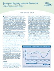
The republic of Zambia is a landlocked country located in Southern Africa bordered by 

eight countries namely: Mozambique, Malawi, Tanzania, Democratic Republic of Congo, 

Angola, Namibia and Zimbabwe (Figure 1.1). The country has a population estimated at 

12.5 million with 65% being rural population and 35% urban population, and has a Gross 

Domestic Product (GDP) per capital of US$1,223 2 . 

Figure 1.1: Geographical Location of the Republic of Zambia 

Zambia 

Source: http://www.worldatlas.com/webimage/countrys/africa/zm.htm 

In Zambia, nearly 90% of all fresh produce marketed in Lusaka 3 flows through traditional 

retail channels, specifically the open air markets and street vendors and other informal 

traders operating outside the market, while modern retail channels such as supermarket 

2 International Monetary Fund (IMF) publications. 

http://www.imf.org/external/pubs/ft/weo/2008/02/weodata 

3 Lusaka is the capital city of Zambia and has the largest FFV wholesale and retailing system. 

4 

Zambia

chains and independent supermarkets hold combined shares of less than 10% (Food 

Security Research Project Urban Consumption Survey, 2007). This clearly tells us that 

the traditional sector dominates the fresh produce system as in most of Sub Saharan 

Africa (SSA). 

In many SSA countries, there has been rapidly rising share of urban population in total 

population. According to the Population Division of the Department of Economic and 

Social Affairs of the United Nations Secretariat, over the past few decades and in the next 

to come, the percent of urban population has been and will continue to rise steadily 

compared to the rural population which is actually decreasing 4 . However, in Zambia this 

has not exactly been the trend. Over the period between 1980 to 2030, the percent of 

urban population had initially been increasing, then it begun to decrease in the 1990’s and 

then steadily rising after 2005 5 . The decreasing annual urban population trend is 

attributed to the investments made in the mining sector which saw a good number of 

people moving to the rural mine areas for employment. 

Considering the overall increase in the urban population in SSA, the traditional marketing 

channels in African horticultural sectors are now subject to heavy pressures for change. 

In Zambia, urban populations are growing rapidly and therefore the traditional 

horticulture systems need substantial investment. Since urban marketing infrastructure in 

most of the continent, Zambia included, has received very little investment in recent 

decades, the result has been often chaotic, unsanitary, and high-cost marketing systems 

4 World Urbanization Prospects: The 2007 Revision Population Database 

http://esa.un.org/unup/p2k0data.asp 

5 http://esa.un.org/unup/p2k0data.asp 

5

that don’t serve the interests of farmers or consumers very well (Hichaambwa and 

Tschirley, 2006). 

Soweto market in Lusaka is the largest wholesale and retail center for fresh fruits and 

vegetables (FFV) in the country. Located in the center of the city, it is a commercial hub 

for FFV and a wide assortment of other food items such as dry cereals, pulses, and tubers, 

among others. Despite the huge amounts of FFV and other food items it handles, this 

market has for a long time been in a poor state. It has poor and limited sanitation, a poor 

waste management system and a poor drainage system. Even though the local council 

authority collects market stall levies from the operators in this market, there has been 

little investments made to improve it. Coupled to its physical inadequacy is the absence 

of market information, and the lack of formal grades and standards. (Hichaambwa and 

Tschirley, 2006, Typsa Consulting Engineers and Architects, 2004) 

In an attempt to address some of the concerns in Soweto market, the European Union, in 

collaboration with the Ministry of Local Government and Housing is currently investing 

over 16 million Euros into a program called the Urban Markets Development Program 

(UMDP). Among other things, the UMDP has focused on the construction of improved 

physical infrastructure in selected markets of Lusaka, Ndola and Kitwe cities. In Lusaka, 

Soweto market is one of the markets that has benefited from this program (Hichaambwa 

and Tschirley, 2006). This program is currently ongoing in all selected markets and 

works in Lusaka’s Soweto market still continue. Despite the investment made by UMDP 

in Soweto market, it is not clear how meaningful a contribution the program will make 

6

towards lowering the costs, encouraging higher quality and better price predictability, 

among other things, for tomatoes and other FFV, and generally improving wholesaling 

and retailing of fresh produce in the market. 

This paper shall focus on the wholesaling and retailing of tomatoes in Lusaka’s Soweto 

market. Among all FFV, tomatoes have the second largest share in both production and 

consumption in Zambia, following rape, (FSRP UCS data, 2007). Tomatoes are therefore 

one the most widely consumed fresh fruits and vegetables. However, farmers, traders, 

and consumers of these tomatoes are faced with tremendous price variability from day to 

day and also within days. Given the high level of variability of tomato prices, two 

important questions arise. Firstly, what is the effect of this variability on the riskiness of 

returns to farmers? And secondly, can market information lead to improved decision 

making that raises and stabilizes returns? This paper shall address these two questions. 

1.2 Objectives of the Study 

The overall objective of this study is to evaluate the price variability of tomato in 

Lusaka’s Soweto market and to assess the effects of different production and marketing 

strategies on farmers’ performance. Soweto market accounts for the lion’s share of 

wholesale fresh produce transactions in Lusaka. 

The specific objectives of the study are: 

1. To identify the level of price variability for tomato in Soweto market and evaluate 

how this compares with other markets around the world. 

7

2. To determine the impact of price variability on the current level and variability of 

farmer returns to tomato production. 

3. To assess the effects of alternative production and marketing strategies, and “generic” 

supply chain improvements on the variability of price and returns to farmers. 

1.3 Organization of Thesis 

The thesis organization is as follows: Chapter 2 gives a detailed overview of the tomato 

production and marketing system serving Lusaka. The data and methods of analysis used 

are also discussed. A tomato subsector channel map is presented with a discussion on the 

various actors in the subsector. 

Chapter 3 presents the hypothesis, an analysis, results and discussion of the tomato price 

variability at wholesale level where a comparison of Soweto market with some other 

wholesale markets in other parts of the world was made. Tomato price variability in 

wholesale markets of the US, Taiwan, Costa Rica and Sri Lanka was analyzed and 

compared with that of Zambia’s Soweto market. 

Chapter 4 presents the data used, results and discussion on the various Monte Carlo 

analyses conducted. Both the conditional and unconditional distribution of the tomato 

growers net returns from tomato production are looked at. The conditional profits 

discussed are based on the tomato grower’s production and marketing decisions and on 

the use of certain market information, while the unconditional profits are based on the 

tomato prices they observe in the market. 

8

Chapter 5 concludes the thesis with a presentation of a summary of the study, policy 

implications, contributions and limitations of the study, and suggestions for future 

research. 

9

CHAPTER TWO 

TOMATO PRODUCTION AND MARKETING SYSTEM SERVING LUSAKA 

This chapter provides a broad and detailed examination of the tomato production and 

marketing system serving Lusaka. It starts by explaining the broad array of data and the 

methods used. It then uses these data to examine fresh produce in consumer budget 

shares across four cities of Zambia. Next, it focuses on Lusaka, presenting an overview 

of the structure of the tomato production and marketing system for the city, organized 

around a detailed tomato channel map that brings together data and information from 

many sources. Key points about the organization of the sector are highlighted in this 

section, and are examined in more detail in subsequent sections. After the overview is a 

discussion of the entire vertical supply chain for the “traditional” sector followed by the 

“modern” sector. In closing, price behavior at the farm, wholesale, and retail levels is 

examined. 

2.1 Data 

The data used in this chapter comes from three sources: the Food Security Research 

Project 6 Urban Consumption Survey (FSRP-UCS), the FSRP wholesale and retail price 

and quantity data, and data on the FFV procurement systems adopted by some selected 

retail outlets and FFV processing firms in Lusaka. 

2.1.1 Urban Consumption Survey Data 

The UCS was conducted in 2007 and it contained household consumption data from 

urban consumers in Kitwe, Mansa, Lusaka and Kasama cities, all in Zambia. This survey 

was collected from a sample size of 2,160 urban consumers who were sampled using a 

6 The Food Security Research Project (FSRP) has operated in Zambia since 1999, with funding from U.S. 

Agency for International Development/ Zambia and, recently, from the Swedish International Development 

Agency. Over the past decade it has collected various household- and market level data sets in 

collaboration with local organizations; some of those data sets are used in this thesis. 

10

andomized cluster sample design. This data contains specific information on the various 

FFV, other food and non-food items purchased and consumed by the household; the 

value of consumption for all the foods purchased, and the primary retail outlet in which 

each item was purchased. In total, there was data collected on 37 FFV and food items 

such as rape, tomato, onion, cabbage, cassava leaves, sweet potato leaves, pumpkin 

leaves, bananas, mangoes, oranges, apples and beans, and nine non-food items such as 

fire wood, paraffin, batteries and vaseline jelly. In addition to this data on the FFV, food 

and non food items, the survey also collected data on household expenditures, the 

households’ participation in urban agriculture (horticultural crop production and livestock 

production) and the households’ food security levels. 

2.1.2 Tomato Wholesale and Retail Price and Quantity Data 

FSRP market reporters collect price data at wholesale and retail, and quantity data at 

wholesale, for tomato, rape, and onions every Monday, Wednesday and Friday. This 

quantity data captures total volumes of tomatoes (and the other two crops) moving 

through Soweto market, while the price data is collected at Soweto and selected retail 

outlets. Soweto market is supplied with tomatoes from over 150 areas from Lusaka and 

Central provinces. Quantity data includes information on the area of origin and the size 

(number of crates) of every lot entering the market. By “area of origin” we refer to a 

production area at the sub-district level as identified by farmers and traders selling in the 

market. A “lot” is defined as the set of crates belonging to an individual farmer or trader 

whose tomatoes are being sold in the market. The Soweto wholesale price and quantity 

data 7 tracks entering 8 , starting and ending volumes of tomatoes in the market from all the 

7 Food Security Research Project: Tomato wholesale and retail price and quantity data. 

11

supply areas. Three price observations are collected and recorded each hour, and the 

mean of the three prices is taken as the hourly tomato price. This is particularly the case 

for the price data on entering volumes. 

Retail outlets where price data is collected are Shoprite (Cairo/Kafue roads), Spar (Down 

town), and Melissa (Matero) supermarket chains, and Chilenje open air retail market. All 

these data have been collected since January 2007; however, in generating the subsector 

map, only data for the one year period January to December 2007 was used. 

2.1.3 Data on Procurement Systems 

Data on the procurement systems of selected retail outlets and FFV processors was 

obtained from interviews with the procurement managers of these institutions. The 

interview guide used for these interviews is presented in Appendix 1. This guide took the 

form of a checklist questionnaire with a combination of closed and open ended questions. 

Open ended questions were included in order to get the broadest possible insights into the 

nature of the procurement systems these actors have adopted. Some of the information 

solicited from the interview included what FFV they trade in, who their FFV suppliers 

are, and more specifically, who their tomato suppliers are, the geographic origin of the 

tomatoes from their suppliers, the quantity and specification requirements of the 

tomatoes, and their tomato pricing policy. The interview was conducted on three large 

independent supermarket chains; Shoprite (Fresh mark), Spar and Melissa, and the two 

main FFV processors in the country; Freshpikt and Rivonia. 

8 Entering volumes are those entering the respective markets between 6am and 1pm; starting volumes refer 

to the volumes of tomatoes entering between the end of the previous day and 6am, while ending volumes 

are those sitting in the market still unsold at noon each day. 

12

2.2 Methods 

With these three sets of data, two types of analysis were conducted. The first involved 

ascertaining the importance of tomato among all the FFV and the second one involved 

the analysis of the tomato subsector which also included some analysis of the 

significance of the traditional retail sector. 

The UCS data was used to ascertain the importance of tomato among all FFV, and also to 

show the significance of the traditional retail sector. Based on household expenditure, the 

first analysis involved calculating: 

- budget shares of all food items purchased, 

- budget share of FFV in overall FFV purchased, and 

- budget shares of all FFV items for Lusaka by income quartiles 

In determining the significance of the traditional retail sector, the analysis involved 

calculating: 

- retail outlet market shares for all food items purchased, 

- retail outlet market shares for tomatoes by expenditure, and 

- retail outlet market shares for all FFV by expenditure quartile groups. 

In conducting the tomato subsector analysis, the tomato wholesale and retail price 

collection data, the UCS data and the data on the FFV procurement systems were used. 

These data provided information on: 

- main actors in the tomato sub sector, 

- volumes of tomatoes from the various identified farm areas, 

- volumes of tomatoes from the retail outlets, 

13

- various channels through which tomatoes pass through before they finally reach 

the retail outlets, 

- volumes of tomatoes which are handled by the traders and their sources, 

- lot sizes of tomatoes from the farmers, and 

- type of first sellers of tomatoes in Soweto market; farmers or traders. 

Volume data on supply areas was used to calculate total supply of tomatoes from each 

area and also the total supplies channeled through the various identified marketing 

channels. 

Data on the lot sizes of tomatoes from different supply areas was used to estimate the 

relative size of the farmers from these supply areas. The lot sizes from the farmers were 

then categorized into terciles. Based on where lot sizes from a particular area fell in the 

tercile groups, each supply area was categorized into three groups from the largest to 

smallest implied farm size. The strength of using this approach of categorizing the supply 

areas is that it gives a good estimate of the size of the majority of famers in a given area. 

However, the down side to this approach is that it may underestimate or overestimate 

actual sizes of the farmers in the supply areas. For instance, several small farmers may 

have been categorized as large farmers merely on the basis of a few large lot sizes of 

tomatoes they delivered to the market, or conversely, a few large farmers may have been 

consistently delivering small lot sizes of tomatoes very often and were subsequently 

categorized as small farmers. In general, however, the implied farmer size and resulting 

classification of production areas that emerged from this exercise agree with the 

14

perceptions of farmers and traders in the market regarding the farm structure in most 

areas. 

To understand the FFV procurement systems of the large independent supermarket chains 

and FFV processors, interviews were conducted with the procurement managers of these 

institutions. 

For the subsector analysis, the UCS provided data on the retail outlets the consumers 

purchase their tomatoes from and the volumes of tomatoes purchased in each retail outlet, 

and information on the tomatoes that were grown and consumed by individual 

households and the tomatoes which were given to the households as gifts. This 

information was obtained by summing up the quantities of tomatoes by each retail outlet 

or source. The main output of the tomato subsector analysis was a subsector map which 

shows all the main actors in the system and the total volumes of tomatoes in each 

identified channel. 

2.3 Fresh Produce in Consumer Budget Shares 

Fresh fruits and vegetables are one of the most widely consumed food items among 

households in Lusaka and the other three surveyed cities (table 2.1). In all four cities, 

vegetables and fruits account for 12% of all purchases. In Lusaka, FFVs are fourth (taken 

together) in budget shares after cereals/staples, meat/eggs and other foods. 

In all four cities, tomatoes and onions are in first place, with an average share of 10% of 

all expenditure on FFV (table 2.2). Clearly, tomatoes are a major FFV consumption item 

and therefore have an important impact on households’ purchasing power. 

15

Table 2.1: Budget Shares for all Food Items Purchased by Households, in Four 

Cities of Zambia 

Food Group 

All 4 

Cities Kitwe Mansa Lusaka Kasama 

------ Share in total food expenditure ------ 

Cereals/ staples 0.22 0.25 0.26 0.19 0.23 

Meat, eggs 0.20 0.17 0.16 0.21 0.18 

Other foods 0.17 0.14 0.16 0.20 0.15 

Non-food items 0.13 0.13 0.13 0.13 0.14 

Fish 0.10 0.09 0.11 0.10 0.12 

Vegetables 0.07 0.10 0.09 0.05 0.08 

Fruit 0.05 0.05 0.05 0.05 0.04 

Legumes 0.04 0.04 0.04 0.04 0.04 

Dairy 0.03 0.04 0.02 0.02 0.03 

Source: Food Security Research Project Urban Consumption Survey Data 2007 

16

Table 2.2: Budget Share of Different FFV items in Overall FFV Purchased by 

Households in Four Cities of Zambia 

Consumption Item All cities Kitwe Mansa Lusaka Kasama 

Tomato 0.10 0.10 0.11 0.10 0.10 

Onion 0.10 0.10 0.10 0.09 0.09 

Rape 0.09 0.09 0.09 0.10 0.09 

Impwa 0.07 0.07 0.06 0.06 0.08 

Cabbage 0.07 0.06 0.06 0.07 0.07 

Sweet potato leaves 0.07 0.07 0.07 0.06 0.07 

Pumpkin leaves 0.06 0.06 0.07 0.06 0.06 

Bananas 0.06 0.06 0.06 0.07 0.05 

Okra (lady's finger) 0.05 0.06 0.04 0.07 0.04 

Oranges/ tangerines 0.05 0.05 0.05 0.05 0.04 

Cassava leaves 0.05 0.05 0.07 0.02 0.04 

Mangoes 0.04 0.04 0.05 0.03 0.04 

Bean leaves 0.03 0.03 0.04 0.02 0.05 

Lemons 0.03 0.04 0.03 0.04 0.02 

Amaranthus (bondwe) 0.03 0.02 0.03 0.03 0.05 

Avocado pear 0.03 0.03 0.02 0.02 0.04 

Apples 0.03 0.03 0.02 0.04 0.01 

Guavas 0.02 0.02 0.01 0.02 0.02 

Green beans 0.01 0.01 0.00 0.03 0.01 

Watermelons 0.01 0.01 0.00 0.01 0.00 

Eggplant 0.01 0.01 0.00 0.01 0.00 

Source: Food Security Research Project Urban Consumption Survey Data 2007. 

Analysis of the budget shares of the different FFV items consumed by the households 

over their total expenditure on FFV, by expenditure quartile was also conducted (Table 

2.3). Using the data on all the food and non-food expenditure items, the households were 

grouped into expenditure quartiles. These quartiles were calculated by first summing all 

household expenditures for food and non-food items. Households were then ordered from 

the highest to lowest total expenditure then broken into four groups of equal size. 

Quartile 1 is the least expenditure group and has a mean total expenditure of ZMK 9 489, 

700, while quartile 4 is the highest expenditure group with a mean of ZMK 3, 867, 700. 

Quartile 2 is the second lowest expenditure group with an average income of ZMK 894, 

9 

The mean exchange rate to the USD during 2007 was (Zambian Kwacha) ZMK 4, 114; Source: 

www.oanda.com 

17

800 and quartile 3 is the second highest expenditure group with a mean expenditure of 

ZMK 1, 508, 205. 

The results show that, tomatoes rank first in the first expenditure quartiles, while tied 

with rape in first rank in the quartiles 2 through 4. Among the households in the third and 

fourth expenditure quartiles, tomatoes had a budget share of 9% of the total FFV 

expenditures of the household while the households in the income quartile 2 and 1 had 

10% and 13% budget share of tomatoes respectively, over all FFV items. Both rape and 

tomatoes have the largest budget share among the relatively poor households (rape forms 

a very prominent part of relish eaten with nshima 10 for these households), they both have 

the same pattern across all the quartiles falling from 13% to 9% for tomatoes, and 12% to 

8% for rape.. This basically shows the importance of tomatoes regardless of the 

household income levels. 

10 

Nsima is a maize meal pulp made from maize flour and is the main staple consumed by households in 

Zambia. 

18

Table 2.3: Budget Share of Different FFV Items in Overall FFV by Expenditure 

Quartile for Households in Lusaka 

Expenditure Expenditure Expenditure Expenditure 

Consumption Item quartile1 quartile 2 quartile 3 quartile 4 

Rape 0.12 0.10 0.09 0.08 

Tomato 0.13 0.10 0.09 0.09 

Onion 0.11 0.10 0.09 0.09 

Cabbage 0.08 0.07 0.07 0.07 

Chinese cabbage 0.01 0.02 0.01 0.01 

Cassava leaves 0.02 0.02 0.02 0.02 

Sweet potato leaves 0.06 0.06 0.06 0.05 

Pumpkin leaves 0.06 0.06 0.06 0.05 

Amaranthus (bondwe) 0.03 0.03 0.03 0.03 

Bean leaves 0.01 0.02 0.02 0.02 

Okra (lady's finger) 0.08 0.07 0.07 0.06 

Impwa 0.06 0.07 0.06 0.06 

Eggplant 0.00 0.01 0.01 0.02 

Green beans 0.02 0.02 0.03 0.04 

Bananas 0.05 0.06 0.07 0.07 

Mangoes 0.03 0.03 0.03 0.03 

Oranges/ tangerines 0.04 0.05 0.06 0.05 

Apples 0.02 0.03 0.04 0.05 

Avocado pear 0.01 0.02 0.03 0.03 

Watermelons 0.01 0.01 0.01 0.02 

Guavas 0.01 0.02 0.03 0.02 

Lemons 0.04 0.03 0.04 0.04 


2.4 The Structure of the Tomato Production and Marketing System Serving 

Lusaka 

This section examines the structure of the tomato production and marketing system 

serving Lusaka. This system is composed of tomato farmers categorized in three areas 

based on the farmer types that dominate the area, tomato assemblers/processors, tomato 

wholesalers, and a wide range of retailers. 

Over 90% of tomato wholesale volume flows through the traditional sector, with less than 

10% volumes flowing through the modern sector comprising Freshmark, which is a 

formal wholesaler and processors Freshpikt and Rivonia. 

19

The retail sector is composed of both informal and formal actors. The informal system is 

composed of open air markets and the “ka sector 11 ”, which refers to all small FFV 

vendors, while the formal system is composed of the large independent supermarkets, 

large chain supermarkets, mini marts and small super markets 

2.4.1 Overview 

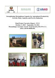
Figure 2.1 presents a simplified channel map for the tomato system serving Lusaka. 

About two-thirds of all tomato in Lusaka comes from areas dominated by large and 

medium size farmers. Also about three quarters of all volume is directly marketed by 

farmers with less than one-fifth of these tomatoes first going through rural traders. 

Travel times from the production areas to Soweto are mostly under 1 ½ hours, with the 

longest times being 4 hours. The market channel for tomatoes arriving into Lusaka is 

therefore actually quite short. Freshpikt is the predominant FFV processor in Zambia and 

it accounts for 8% of the tomatoes in the system all of which it produces on its own. 

Over 80% of tomatoes from farmers end up in Soweto market with less than 10% going 

to Bauleni market. Soweto market clearly dominates as the main wholesale entity in 

Lusaka. The processing and modern wholesaling sectors, dominated by Freshpikt 

(Freshmark and Rivonia have extremely small shares) take less than 10% of the market. 

In the retailing section, the traditional sector dominates with over 90% of the market. 

11 The “ka sector” refers to the informal retail outlets for FFV and these include market stands, market stall 

vendors, mobile vendors, street vendors, ka table (small table stall), kantemba (small rudimentary shop) 

and ka shop (kiosk) (FSRP Urban Survey Training Manual, 2007) 

20

Figure 2.1: Channel Map for Tomato Systtem 

Serving Lusaka 

21 

Grocery/Mini-Mart (2%) 

Private HH & Gifts (2%) 

Large S Indpt (

2.4.2 The “Traditional” Sector 

The traditional wholesale sector is made up of Soweto and Bauleni markets which 

together have an overall market share of 91% at this level. At retail, the traditional sector 

has a 92% market share and is composed of the open air markets and the ka sector. These 

results clearly show how both the wholesale and retail traditional sectors dominate the 

tomato subsector. 

Soweto market is the main wholesale channel through which tomatoes pass before they 

reach the various retail outlets. This market is supplied by a wide range of geographic 

areas that include small, medium and large farm areas. Bauleni market on the other hand 

is a small wholesale market that has much of its tomato supplied by farmers in small farm 

areas, specifically from Manyika in Chongwe district. Bauleni market is on the from this 

area to Soweto market, and as such, quite often farmers from Manyika would opt to sell 

their tomatoes in this market when they have smaller quantities which can easily be 

purchased in this market, thus making proceeding to Soweto market unnecessary. 

i. Production Areas 

The FSRP price and quantity data base described earlier identifies 150 distinct areas that 

supplies Lusaka with tomato during 2007. Of these, the twelve main geographical areas 

that produce and supply tomatoes to Soweto market are Chalimbana, Chisamba, Choona, 

Lusaka West, Makeni, Masansa, Manyika, Mkushi Farm Block, Mwaalumina, 

Mwembeshi, Nkolonga and a special grouping of farmers from Kapiri Mposhi district 

(table 2.4). These twelve areas account for 68% of the tomato supplies that reached 

Soweto market during 2007. 

22

Table 2.4: Key Characteristics of Tomato Production Areas Supplying Lusaka in 2007 

Farmer Size 

Mean Decile 

Weighted 

Average Price 

Market Median Lot Ranking of lot 

Seasonality (Supply Received 

Area Province share Size (mt) size months) 

(ZMK/kg) 

1 

Farmer 

Description 

Lusaka West Lusaka 0.104 1.12 5.78 All types of 

farmers: farmers are 

almost evenly 

spread out across all 

deciles but with 

modes in the 7 th and 

9 th Most sales during low price 1,024 

period of May to September 

2007, short peak during high 

deciles. 

price month of February 2007 

Masansa Central 0.098 1.96 6.84 Large farmers: most Highest sales March/April 1,262 

of the farmers are in 2007, straddling high and low 

the top three price months; also November 

deciles. 

2007 (high price) and 

March/April 

price). 

2008 (low 

Chisamba Central 0.082 1.96 7.01 Large farmers: the Sales are mostly concentrated 1,013 

majority of the in the low price months - May 

farmers are in the to July 2007, with another 

top two deciles. sales peak during high price 

months - November & 

Choona Central 0.07 0.59 4.15 Small farmers: most 

December 2007 

Caught end of high price 1,118 

of the farmers are in period in March and early 

the lower deciles. April 2007, but otherwise 

sales concentrated in low 

price months of April/May 

2007 and March-April 2008. 

23

Table 2.5 cont’d 

Area Province Market 

share 

Farmer Size Seasonality (Supply 

months) 

Manyika Lusaka 0.061 0.7 4.59 Small farmers: most farmers are 

in the low deciles. 

Mwembeshi Lusaka 0.05 1.12 5.77 All types of farmers: the farmers 

are almost evenly spread out in 

all deciles with the 5th and the 

9th deciles having more 

observations. 

Makeni Lusaka 0.048 0.67 4.41 Small farmers: most of the 

farmers are in the lower deciles. 

Chalimbana Lusaka 0.047 1.31 6.01 All types of farmers: the farmers 

are almost evenly spread out 

across all deciles but with mode 

Mkushi 

Farm Block 

in the 7th and 8th deciles. 

Central 0.043 2.81 7.27 Large farmers: most of the 

farmers are in the top two 

deciles. 

24 

Highest sales during high 

price month of February 

2007, also December 2007 to 

January 2008, but maintained 

a substantial amount of sales 

in the low price period of 

March 2007 to August 2007. 

Sales heavily concentrated in 

low price months – May to 

September 2007. 

Sales heavily concentrated in 

low price months of July to 

September 2007. 

Low price months - June to 

Aug 2007. High price month 

– December 2007 

Most sales concentrated 

during high price months – 

February to March 2007 and 

December 2007 to February 

2008. 

Weighted 

Average Price 

Received 

(ZMK/kg) 

1,093 

928 

921 

945 

1382


Area Province Market 

share 

Farmer Size Seasonality (Supply 

months) 

Nkolonga Central 0.031 2.36 7.54 Large farmers: most 

of the farmers are in 

the top three 

Farmers in 

Kapiri 

Mposhi 

district 

deciles. 

Central 0.027 2.25 7.27 Large farmers: most 

of the farmers are in 

the top four deciles. 

Mwalumina Lusaka 0.022 1.16 5.78 Medium farmers: 

most farmers are 

located in the 

median deciles 

between 5 and 8 

with more in the 8th 

Average for 

all areas 

25 

Nearly all sales occurred 

during high price months – 

November 2007 to January 

2008. 

Most sales during high price 

months – October to 

November 2007, January 

2008, and January to 

February 2007. 

Main peak during low price 

months of June to September 

2007; second peak high price 

months of December 2007 to 

January 2008. 

Weighted 

Average Price 

Received 

(ZMK/kg) 

1,168 

- 0.68 - - 

decile. 

- - 1,079 

Source: Food Security Research Project – Tomato Supply data 2007/2008 

1 1 is the smallest possible mean decile and 10 is the largest possible mean decile. 

1,372 

890

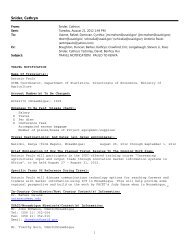
Monthly wholesale prices per kilogram of tomato in Soweto market for the period 

between January 2007 and June 2008 were analyzed (figure 2.1). From the figure, over 

the 19 month period it was observed that there are a number of high and low price 

months and also sudden price drops which are a concern. The notable high price months 

during this period are February to March 2007, October and November 2007, and 

January 2008 and February 2008, while the low price months were around April to 

August 2007, December 2007 and March 2008. A closer examination of the seasonality 

during January through June in both years reveals that at the beginning of both years the 

prices are fairly high and then there is a sudden price collapse. In 2007, the price collapse 

occurred in April while the 2008 price collapse occurred in March. 

26

Figure 2.2: Monthly Soweto Wholesale Tomato Prices January 2007 to July 2008 

Price per Kg (ZMK/kg) 

2000.00 

1500.00 

1000.00 

500.00 

Source: Food Security Research Project – Tomato price data 2007/2008 

JAN FEB MAR APR MAY JUN JUL AUG SEP OCT NOV DEC JAN FEB MAR APR MAY JUN JUL 

2007 2007 2007 2007 2007 2007 2007 2007 2007 2007 2007 2007 2008 2008 2008 2008 2008 2008 2008 

Among the top twelve supply areas, those that supplied tomatoes to the market in both 

Date 

high and low price months are Lusaka West, Manyika and Mwalumina. Farmers in areas 

like Mkushi farm block, Nkolonga and Kapiri Mposhi district supplied their tomatoes 

mainly in the high price months. In the low price months, the dominant supply areas were 

Masansa, Chisamba, Choona, Mwembeshi, Makeni and Chalimbana. 

Judging by the quantities of tomato that were supplied from the various supply areas in 

April 2007, Masansa, Choona, Manyika and Lusaka West had the highest volumes of 

tomatoes in that period (298mt, 182mt, 75mt and 75mt respectively) and accounted for 

59% of the tomatoes on the market. On account of this, their supplies are likely to have 

been the main cause of the April price collapse 

27

In the case of the March 2008 price collapse, Choona and Masansa collectively supplied 

the market with 49% of the tomatoes. Choona alone accounted for 20% and supplied the 

market with 247 mt while Masansa supplied 174 mt. The supplies from the two areas are 

to some extent largely responsible for the March price collapse. 

As noted earlier, supply areas such as Mkushi farm block, Nkolonga and farmers in 

Kapiri Mposhi district supplied the market with tomatoes mainly during high price 

months. These supply areas are dominated by large farmers who generally have more 

financial resources and farming knowledge than small farmers. The high price months 

these farmers supplied their tomatoes in is indicative of a tomato crop grown in the rainy 

season, during which production costs can be very high. These high production costs are 

associated with high weed management requirements and more frequent pest and disease 

outbreaks which require chemical applications for their management. Being large 

farmers, it is easier for them to grow and manage a rain fed crop since they have more 

financial resources to engage labor for weeding and buy chemicals for pest and disease 

control. In addition to this, with the edge they have in farming knowledge, this puts them 

in a better position to manage their crops well. 

On the basis of the different supply areas and the different farmer types found in each 

supply area, the channels through which tomatoes enter the system is presented in figure 

2.1. Channels 1 through 3 represent tomatoes taken directly to the markets by farmers 

28

from all 150 supply areas while channels 4 through 6 represent tomatoes that were first 

sold to traders. 

Channel 1 represents the flow of tomatoes from small farm areas into Soweto market. 

Among the top twelve supply areas, channel 1 was made up of famers from Choona, 

Manyika and Makeni. This channel has a 19% share of tomatoes entering Soweto market. 

The Soweto data on the origin of tomato supplies shows that the majority of the farmers 

in this channel are located in the lower deciles with only a few in the top two deciles. 

Farmers in this area mainly supplied their tomatoes to Soweto market in the low price 

months of March to May 2007 and March of 2008. 

The medium farm area is represented by channel 2 and among the top 12 supply areas 

had farmers from Lusaka West, Mwembeshi, Chalimbana and Mwalumina. A large 

number of farmer observations are well distributed in all the deciles with the majority of 

them lying in the 5 th and 9 th deciles. The farmers in this channel account for 28% of the 

tomato volumes in Soweto market. This area supplied most of its tomatoes in the low 

price months of May to September 2007. 

The large farm area is represented by channel 3 and among the top 12 supply areas had 

farmers from Masansa, Chisamba, Mkushi farm block, farmers in Kapiri Mposhi district 

and Nkolonga. Most farmers in this area are concentrated in the top four deciles. About 

19% of the tomatoes in Soweto market are from this area, and most of their tomatoes 

29

were supplied in the high price months of February to April 2007 and December 2007 to 

January 2008. 

Eighteen percent of the tomatoes that enter Soweto market come through traders 

(Channels 4-6). The tomatoes from the traders are originally from the farm areas but are 

channeled through these intermediaries before they finally reach Soweto market. Channel 

4 represents the tomatoes that come from the small farm areas to the traders, while 

channel 5 represents tomatoes from the medium farm areas to the traders and finally 

channel 6 representing tomatoes from the large farm areas to the traders. 

Tomatoes from the different supply areas are then wholesaled in Soweto and Bauleni 

markets and then eventually channeled out to the retail outlets. Among the various retail 

outlets are the open air markets which account for 67% of the volumes of tomatoes, 

followed by the Ka sector with 24%, with the remaining 9% being transacted in the 

grocery mini marts (5%), large super market chains (

Table 2.7: Retail Outlet Market Shares on Overall Food (Lusaka) 

Market Group /Retail Share for Share for Share for Share for Share for 

Outlet 

all foods all FFV Vegetables fruits tomatoes 

Open Air Market 0.32 0.55 0.64 0.45 0.67 

Ka Sector 0.16 0.20 0.20 0.21 0.24 

Grocer / Mini mart 0.21 0.01 0.02 0.003 0.05 

Own Production 0.02 0.09 0.07 0.13 0.01 

Private HH 0.02 0.01 0.01 0.01 0.01 

Gift 

Large Independent 

0.03 0.06 0.04 0.09 0.01 

Supermarkets 0.01 0.01 0.01 0.01 0.01 

Large Supermarket Chains 0.09 0.05 0.02 0.09 0.003 

Butcher 0.14 0.00 0.00 0.00 0.00 

Small Supermarkets 0.01 0.001 0.001 0.001 0.00 

Other Purchasing Channel 0.01 0.00 0.00 0.00 0.00 

Baker 0.001 0.00 0.00 0.00 0.00 


The broader literature 12 on supermarket expansion in the developing world shows that the 

general pattern of their development has mainly been through the spread of foreign direct 

investment (FDI). Zambia is no exception. Much of the FDI in supermarkets in Zambia 

is from South Africa where the supermarket share of the national food retail is 55% 13 . 

The shares in South Africa are similar to those found in some Latin American countries 

such as Argentina and Chile 14 . In Zambia however, the growth rate of these supermarkets 

has not been as fast as in these parts of the world and hence the small share they have in 

the retail outlet markets. 

Further analysis on the retail outlet market shares for all FFV purchases made by the 

households by the expenditure quartiles was conducted, and the results show that the 

traditional retail still ranks highest among all the retail outlets used by all the expenditure 

quartile groups (Table 2.6). In the two lowest income quartiles, the open air markets and 

12 Reardon and Timmer, 2006; Tschirley 2007 

13 Weatherspoon and Reardon, 2003. 

14 Weatherspoon and Reardon, 2003. 

31

the ka sectors combined have shares of over 90%, while the top two income quartiles (3 

and 4) have shares of at least 80%. Households in the highest income quartile tend to use 

the formal retail outlets (specifically the small supermarkets and the large supermarket 

chains) more than the other income quartile groups. 

Table 2.8: Retail Outlet Market Shares for all FFV Purchases by Income Quartile 


Market group/Retail outlet quartile 1 quartile 2 quartile 3 quartile 4 

Open Air Market 0.67 0.70 0.62 0.53 

Ka Sector 0.26 0.22 0.26 0.27 

Grocer / Mini mart 0.002 0.002 0.009 0.037 

Small Supermarkets 0.00 0.00 0.001 0.001 

Large Independent supermarkets 0.00 0.00 0.00 0.01 

Large Supermarket Chain 0.002 0.004 0.02 0.06 

Butcher 0.00 0.00 0.00 0.00 

Baker 0.00 0.00 0.00 0.00 

Private household 0.01 0.02 0.02 0.02 

Other Purchasing Channel 0.00 0.00 0.00 0.00 

Own Production 0.02 0.03 0.05 0.06 

Gift 0.02 0.02 0.02 0.02 


An examination of the retail outlets shares for tomatoes by expenditure quartiles, also 

reveals that the open air markets and the ka sectors combined have the largest retail outlet 

market share (Table 2.7). The highest income quartile has a combined retail outlet market 

share of 85% in the open air markets and the ka sector while the other income quartiles 

all have over 90% share. The highest income quartile are the main group that use the 

grocery/mini mart and large independent supermarkets for the purchase of tomatoes with 

shares of 7% and 1% respectively. 

32

Table 2.9: Retail Outlet Market Shares for Tomato Purchases by Expenditure 

Quartile 


Market group/Retail outlet quartile 1 quartile 2 quartile 3 quartile 4 

Open Air Market 0.58 0.64 0.65 0.55 

Ka Sector 0.37 0.28 0.30 0.30 

Grocer / Mini mart 0.00 0.00 0.002 0.07 

Small Super markets 0.00 0.00 0.00 0.00 

Large Independent Super markets 0.00 0.00 0.00 0.01 

Large Supermarket Chain 0.00 0.00 0.003 0.00 

Butcher 0.00 0.00 0.00 0.00 

Baker 0.00 0.00 0.00 0.00 

Private households 0.03 0.03 0.03 0.04 

Other Purchasing Channel 0.00 0.00 0.00 0.00 

Own Production 0.01 0.03 0.01 0.01 

Gift 0.02 0.02 0.00 0.01 


Evidently, the informal sector comprising the open air markets and the ka sector are very 

important. The formal sector has a very low percentage share for the transaction of FFV 

and especially for tomato, despite the manner in which it is well organized and the 

infrastructure in place. In view of the high percentage share of FFV transactions 

occurring in the two identified informal channels, it would be paramount to ensure that 

the performance of this sector is enhanced by way of identifying means through which 

there would be a more efficient handling of the volumes of FFV that pass through it. 

2.4.3 The ‘Modern’ Sector: Supermarkets and Processors 

The modern sector of the tomato system is composed mainly of supermarkets and 

processors. The supermarkets that dominate this sector are Shoprite, Melissa and Spar 

while the processors include Freshpikt and Rivonia. The supermarkets and the processors 

in this sector jointly have a 9% share in the tomato system. The following section gives 

33

some details of these supermarkets and processors and also looks at the tomato 

procurement system they have adopted. 

i. Shoprite Supermarket/Freshmark 

Freshmark serves as a wholesale procurement and distribution channel for tomatoes 

supplied to all 17 Shoprite retail outlets countrywide. Shoprite is the largest super market 

chain in Zambia and mainly relies on Freshmark for all its FFV requirements. It however 

handles less than one percent of the tomatoes consumed in the country. 

In its tomato procurement system, Freshmark currently has four farmers that supply it 

with tomatoes; three commercial farmers and one small scale farmer. All of these farmers 

are located in Lusaka province. The small farmer is located in Makeni, South of Lusaka 

city. One of the large commercial farmers is located in Chisamba area while the other two 

are South of Lusaka city in Kafue area. 

Ninety percent of the tomatoes supplied to Freshmark come from the three commercial 

farmers and the remaining 10% comes from the small scale farmer. Ambrosia farm 

accounts for 40% of the supply while the other two commercial farmers account for the 

remaining 50% with each one supplying approximately 25%. 

To qualify as a tomato supplier to Freshmark, the suppliers have to adhere to a number of 

quality standards that are above what would be expected in an open air market. Some of 

Freshmark’s quality requirements are, firm, champagne red color tomatoes, free of any 

blemishes and able to have a shelf life of 3 days at the time of delivery. 

34

Freshmark mostly prefers to have large farmers as tomato suppliers as they are more 

reliable and stick to the terms and conditions of the contracts they enter into. The 

procurement manager indicated that small farmers, other than having production 

constraints which hinder them from supplying required quantities and their inability to 

produce a product that meets Freshmark’s quality requirements, have a tendency to break 

the contracts and supply a market that offers a better price at a given point in time. The 

small farmer that currently supplies tomatoes to Freshmark is a very committed farmer 

but has land area limitations that hinder him from expanding his tomato production. 

In cases where the local tomato suppliers are not in a position to meet Freshmark’s 

demand, Freshmark outsources tomatoes from Freshmark South Africa. This is 

particularly the case in the rainy season when the local tomato supplies are very low and 

prices high. 

An average of 4 mt of tomatoes is supplied to the various Shoprite retail outlets every 

week. Seventy-five percent of these tomatoes end up in Lusaka while the remaining 25% 

go to the Shoprite retail outlets outside of Lusaka. Tomatoes are very important in the 

vegetable procurement system as they rank second from potatoes in sales volumes, and 

rank fourth in Shoprite’s overall FFV supply system with bananas, potatoes and apples 

taking the lead in this order. 

Freshmark usually seeks to maintain stable prices during the course of the year. To 

achieve this, the contracted farmers are offered less variable prices for their tomatoes for 

35

the whole one year contract period they enter. Due to this pricing policy, during the peak 

supply season when the tomato prices are generally lower Freshmark offers its farmers 

higher prices than what the market is offering, and when the tomatoes are in short supply 

and prices expected to be higher, Freshmark’s prices would be lower. It is during the high 

market price period that most contracted farmers (particularly the small ones) would 

default and sell their tomatoes where the price is higher. 

ii. Melissa Supermarket 

Melissa supermarket is a Zambian grocery store chain with three outlets in Lusaka city 

located in Northmead, Kabulonga and Matero. The Matero outlet is the most recently 

opened and forms the focus of the following discussion. 

Among all the FFV products purchased by Melissa, tomatoes are important, however 

onions top the list in importance. Melissa has an internal procurement system for 

tomatoes with contractual arrangements with three commercial farmers, Eco Veg, Agir 

Link and Lilayi farms. Each of these farmers supplies Melissa with an assortment of 

FFV, but only Eco Veg supplies them with tomatoes. 

In addition to procuring tomatoes from the commercial farmer, Melissa also obtains some 

from small independent farmers. These independent farmers are basically walk-in 

suppliers without contracts with Melissa, but meet the quality requirements for firm, semi 

ripe, blemish- free tomatoes. Melissa has therefore adopted a dual procurement system 

which enables it to cushion the effects of price fluctuations and unstable supplies. 

36

With the dual procurement system that it has adopted to manage the supplies of tomatoes 

from both sources, Melissa supermarket ensures that it has a weekly tomato supply of 

350 kg. Eco Veg supplies them with tomatoes on Mondays, Wednesdays and Fridays 

while the other suppliers supply the tomatoes on the other days. 

Melissa supermarket has a fixed price arrangement with Eco Veg over each contract 

period, which may vary from a few months to one year. During the contract period, 

irrespective of whether the market price of tomatoes drops or rises, Melissa supermarket 

pays Eco Veg only the agreed amount. In periods when the supply of tomatoes on the 

market is high and the market price lower than the negotiated price with Eco Veg, 

Melissa procures most of its tomatoes from the other suppliers (small independent 

farmers). On the other hand, when the supply of tomatoes on the market is low and the 

market price is higher than the negotiated price with Eco Veg then Melissa procures most 

of its tomatoes from Eco Veg. This procurement arrangement enables Melissa to keep its 

prices fairly stable over a given period of time. With supplies from both sources, Melissa 

averages out the prices received; given the fixed price from Eco Veg and the variable 

price from the other suppliers which may be lower or higher than the Eco Veg price. 

Melissa is comfortable with this dual supply system and does not have any preference for 

either. The benefits of having such a system are better than having one supply source. 

Considering the tomato supplies from the farmers, Melissa supermarket has preference 

for supplies from large farmers as their quality of tomatoes is better than what is obtained 

from the smaller farmers. 

37

iii. Spar Supermarket 

Spar supermarket is the newest supermarket chain in Zambia with its origins in the 

Netherlands. The first Spar retail outlet was opened in 2004. It currently has six outlets 

countrywide; two in the Southern province towns of Livingstone and Choma, and four in 

Lusaka province: Downtown Spar, Soweto Spar, Arcades Spar and Chawama Spar which 

was just recently opened in mid 2008. 

Each of the Spar outlets is run as an independent operation by its own manager, and each 

with its own FFV procurement system and pricing policy. Downtown Spar markets a 

wide range of vegetables such as carrots, peppers, onions, cucumbers, tomatoes, potatoes, 

green beans, and others. Most of the vegetables and other fresh produce they sell come 

from three large farms: Buyabamba farm, Osuma farm and Birchwood farm. The large 

farms account for 60% of the vegetables they are supplied with while the remaining 40% 

is supplied by small farmers and independent traders who deliver the tomatoes to their 

premises. 

On a weekly basis, downtown Spar sells an average of 125kg of tomatoes. To ensure that 

they have a steady supply of tomatoes throughout the year, the store heavily relies on 

Buyabamba farm which consistently has tomatoes throughout the year. 

iv. Freshpikt 

Freshpikt is the dominant FFV processing firm in the country. At present, it produces its 

own tomatoes and supplies its processed products to the grocery mini-marts, large 

supermarket chains, the large independent supermarket retail outlets and exports 5%. 

38

Compared to Soweto market which had an 83% share of raw tomatoes in the system, 

Freshpikt had an 8% share for raw tomatoes in 2007. 

Freshpikt produces 18 different canned products which include baked beans, mixed 

beans, tomato puree, tomato paste, tomato and onion mix, whole peeled tomatoes and an 

assortment of fruit chunks, jams and juices from pine apples. Tomatoes, beans, sweet 

corn and onions are the main vegetables they process and tomatoes are the major 

ingredient used in most of their salty canned products. 

Freshpikt currently sources all of its tomatoes from its own 40 ha farm plot in Lusaka 

East. At 50 mt per week, all year round, the plant is operating well below its capacity of 

60 mt per day. It has plans to step up its processing volumes for tomato products once it 

engages small tomato grower cooperatives on a contractual basis in its supply chain. 

v. Rivonia 

Rivonia is another FFV processing firm specialized in the production of tomato sauces. 

They use local raw tomatoes and imported tomato paste for their sauces. They currently 

procure 540 Kg of tomatoes per week from independent tomato growers in Lusaka 

province. At present, the volumes of tomato that come from the farm areas to Rivonia 

have a share of less than 1% in the system. As with Freshpikt, its processed products end 

up in grocery mini marts, large supermarket chains and the large independent 

supermarket retail outlets. 

39

Mean price /kg 

2.5 Price Behavior 

2.5.1 Weekly Wholesale Prices in Soweto Market 

Soweto market is the main wholesale market in Lusaka and serves as the main source of 

tomatoes for most of the retail outlets in the city. The graph presented below shows the 

weekly wholesale per kg tomato prices that prevailed in Soweto market over the period 

Jan 2007 to July 2008. These are the prices received by farmers and traders selling in the 

market. 

Figure 2.3: Weekly Soweto Wholesale tomato prices January 2007 to July 2008 

3000.00 

2500.00 

2000.00 

1500.00 

1000.00 

500.00 

0.00 

3 9 15 21 27 33 40 46 52 5 11 17 23 26 

WK WK WK WK WK WK WK WK WK WK WK WK WK WK 

07 07 07 07 07 07 07 07 08 08 08 08 08 08 

Source: Food Security Research Project – Tomato price data 2007-2008 

40 

Week

During this period, tomato prices were quite variable in Soweto market. It was observed 

that, despite strong seasonal patterns, there is a fair amount of price variation within a 

given season. A notable feature in the graph over the whole period is the sharp price 

declines experienced in April 2007 (15 Wk 07), December 2007 (49 Wk 07), March 2008 

(11 Wk 07) and June 2008 (25 Wk 08). 

2.5.2 Weighted Average Prices by Marketing Channel 

Going by the channels identified in the channel map (Figure 2.1), table 2.8 shows the 

weighted average prices for a kg of tomatoes in each of these channels. Taking a look at 

the channels for tomatoes that get into Soweto from the farm areas, it can be observed 

that the farmers from large farm areas (channel 3) received the highest prices of ZMK 

1,138 followed by farmers in the small farm areas (channel 1), ZMK 1,055 and finally 

farmers in the medium farm areas (channel 2) receiving ZMK 1,007. 

Interestingly, when we look at the channels for tomatoes that pass through the traders 

before they reach Soweto market, we observe a similar price pattern. The tomatoes sold 

by traders buying form the large farm areas (channel 6) are sold at the highest price, 

ZMK 1,223, followed by those sold by traders buying from small farm areas (channel 4, 

ZMK 989) and finally from traders buying from the medium farm areas (channel 5, ZMK 

932). 

41

Table 2.10: Weighted average tomato prices by market channel 

Channel 

Weighted Avg. Price 

Number Channel Description 

(ZMK) 

6 Sales by traders buying from large farm areas 1,223 

3 Direct farmer sales into Soweto from large farm areas 1,138 

1 Direct farmer sales into Soweto from small farm areas 1,055 

2 Direct farmer sales into Soweto from medium farm areas 1,007 

4 Sales by traders buying from small farm areas 989 

5 Sales by traders buying from medium farm areas 932 


2.5.3 Tomato Wholesale and Retail Prices 

A comparison of tomato prices for Soweto market and four selected retail markets, 

namely Spar, Shoprite and Melissa supermarkets, and Chilenje open air market, was 

made by examining the price trend over the period between January 2007 and July 2008 

(figure 2.4) We observe that Soweto wholesale prices for tomatoes for the whole period 

averaged ZMK 1179, while the retail prices in the selected retail markets were ZMK 

3,450 for Chilenje open air market, ZMK 3,545 for Melissa supermarket, ZMK3,408 for 

Spar supermarket and ZMK 3,390 for Shoprite supermarket (table 2.9). 

42

Figure 2.4: Tomato Pricing at Wholesale and Retail Level 

Week 

07 07 07 07 07 07 07 07 07 07 07 07 07 07 07 07 07 07 07 07 07 07 07 07 07 07 08 08 08 08 08 08 08 08 08 08 08 08 08 08 

Market 

--- Soweto, Lusaka 

A – - Chilenje 

Melissa, Lumumba 

Shoprite, Cairo 

Spar 


43

On the basis of these mean weekly prices observed for these markets (figure 2.4), we see 

that Chilenje market followed a very similar price pattern as Soweto market. Much of the 

tomatoes in Chilenje market are obtained from Soweto market and the prevailing prices 

in Chilenje reflect a fairly stable price mark up averaging ZMK 2,284 per kilogram of 

tomato. To demonstrate the fairly stable price margin over the period, the price margin 

was graphed (figure 2.5). However, in mid March and late June (Week 13 and 25 

respectively) there were price margin spikes experienced in Chilenje market. In these 

periods, Soweto market experienced some price drops and despite these price drops, 

Chilenje market seems to have maintained their price mark ups thereby resulting in the 

high price margin. 

Melissa supermarket maintained a fairly stable price over the period with the tomato 

price averaging ZMK3,545 per kilogram. Shoprite on the other hand seemed to follow 

the traditional retail market (Chilenje) prices in a stepwise fashion. 

Of all four retail markets evaluated, Spar supermarket had the most stable year round 

prices for tomato at a mean price of ZMK 3,400 for most of the year. In both the peak 

and low supply periods, it maintained this stable price with the exception of the low 

supply period of January when it had a low price of ZMK 2,700. 

44

Table 2.11: Mean Tomato Prices for Wholesale and Retail Outlets in Lusaka 

(January 2007 to July 2008) 

Outlet Type of outlet Mean tomato price 

(ZMK) 

Soweto Wholesale 1179 

Shoprite supermarket Retail 3390 

Spar supermarket Retail 3408 

Chilenje open air market Retail 3450 

Melissa supermarket Retail 3545 

Source: Food Security Research Project – Tomato price data 2007/2008 

45

Figure 2.5: Price Margin for Chilenje Retail Market 

5000.00 

4000.00 

3000.00 

2000.00 

Chilenje price margin (Zkw/kg) 6000.00 

1000.00 

3 

WK 

07 

6 

WK 

07 

9 

WK 

07 

12 

WK 

07 

15 

WK 

07 

18 

WK 

07 

21 

WK 

07 

24 

WK 

07 

27 

WK 

07 

30 

WK 

07 

33 

WK 

07 

37 

WK 

07 

40 

WK 

07 

46 

43 

WK 

07 

Date 

46 

WK 

07 

49 

WK 

07 

52 

WK 

07 

2 

WK 

08 

5 

WK 

08 

8 

WK 

08 

11 

WK 

08 

14 

WK 

08 

17 

WK 

08 

20 

WK 

08 

23 

WK 

08 

26 

WK 

08

2.5 Summary and Conclusions 

2.5.1 Importance of Tomatoes 

Fresh fruits and vegetables are a major food item purchased by households in Lusaka, 

Kitwe, Mansa and Kasama urban centers. In all these cities, the budget shares for all food 

items purchased by the households shows that FFV are an important food item as they 

rank third after cereals/staples and meat/eggs respectively. Detailed examination of the 

specific FFV items consumed by the households reveals that tomatoes rank first in the 

FFV budget shares, with almost 10% of the expenditure on all FFVs going to tomatoes. 

Further examination of the budget shares for tomatoes over all FFV by expenditure 

quartiles in Lusaka also reveals that tomatoes rank high in expenditures taking up an 

average of 10% of the FFV budget for households. 

Based on these results, it is clear that tomatoes are an important FFV item and that takes 

up a substantial amount of the consumers’ incomes, thereby impacting on the 

households’ purchasing power. 

2.5.2 The Tomato Subsector 

The tomato subsector in Lusaka is made up of tomato farmers, traders, wholesalers, 

processors/assemblers, and retailers. The farmers supplying tomatoes in the system are 

from large, medium and small farm areas, however, the large and medium farmers 

dominate the system and supply about two thirds of the tomatoes in the system. 

Among the wholesalers, processors/assemblers and retailers in the tomato subsector, 

these actors make up the traditional sector and the modern sector of the tomato subsector. 

47

The traditional sector refers to the informal sector which is mainly made up of the 

Soweto and Bauleni markets, and accounts for over 90% share of tomato volumes at 

wholesale level. At retail level, we have the open air markets and the ka sector which 

collectively account for 91% of the retail sector. The modern sector, on the other hand is 

a formalized sector of the tomato subsector. It is comprised of the FFV processors, 

Freshpikt and Rivonia, and Freshmark, a large wholesale operator. At retail level, the 

modern sector is made up of the large independent supermarkets, the large supermarket 

chains, mini marts and small supermarkets. 

Atleast sixty six percent of all tomatoes entering Soweto market are directly marketed by 

farmers, while 18% are marketed through traders. Traders buy the tomatoes either at the 

farm gate, then transport and sell them in Soweto, or from the farmers at Soweto market 

then sell them to wholesalers there. Eight percent of the tomatoes from the farm areas 

were sold directly to the wholesalers in Bauleni market, and less than 1% was sold to 

Freshmark wholesalers and Rivona. The remaining tomatoes in the system are grown by 

one of the FFV processing firms, Freshpikt. 

Farmers from twelve main geographic areas dominate the system and account for 68% of 

all the tomatoes in the system; the other 32% was split among over 150 other supply 

areas. These farmers supplied tomatoes to Soweto market at different times of the year 

with some of them predominately supplying them in the low price months while others 

supplied them in the high price months. 

48

In the period January 2007 to June 2008, tomato prices were quite variable, and some of 

this variability in the prices was the normal price variability one would expect due to 

seasonality of production. Notable high price months for tomatoes over this period were 

in February to March 2007, September and November 2007, and December 2007 to 

February 2008. The observed low price months were around April to August 2007, 

November 2007 and March 2008. Also worth noting were the sudden price collapses that 

were experienced in April 2007 and March 2008. 

Analysis of the farmers that supplied tomatoes in the market reveals that among the top 

twelve supply areas, the areas Masansa, Choona, Lusaka West and Manyika are partly 

responsible for the price collapse experienced in April 2007. These four areas supplied 

59% share of tomato volumes during this period. In the case of the price collapse that 

occurred in March 2008, farmers from Choona and Masansa may have caused it as they 

account for 49% of the tomatoes in the market at that time. 

Once the tomatoes from the different supply areas arrive in the wholesale markets, they 

are then channeled out to the consumers through the various retail outlets. The traditional 

retail sector, comprising the open air markets and the ka sector dominate the retail 

market, with 91% share. Analysis of the UCS also shows that the traditional retail sector 

dominates with over 90% of FFV sales occurring in it. Further examination of the retail 

outlets used for FFV purchases by income quartile groups also shows that the traditional 

retail sectors dominates with very few purchases being made in the modern sector 

supermarkets. 

49

The modern sector is mainly made up of supermarkets and processors which jointly have 

a 9% share in the tomato system. Shoprite, Spar and Melissa are the dominant 

supermarkets while Freshpikt and Rivonia are the main FFV processors. 

The analysis conducted in this chapter has shown that tomatoes are an important FFV 

item among urban consumers in Zambia. It has also further shown us the dominance of 

both the wholesale and retail traditional sectors of the tomato subsector. Given the 

dominance of the traditional wholesale and retail sector in the tomato sub sector, and the 

poor infrastructure that exists, particularly in Soweto wholesale market, it is important 

that particular attention be paid to them so that they are better able to serve the needs of 

both the sellers and the consumers. Some of the key areas that need improvement for the 

better function of these systems are in the improvement of market infrastructure (roads, 

physical buildings, sanitation, and drainages), market information and cold chains. 

Therefore, developing these markets has the potential to increase the incomes of farmers 

due to the efficiency that would result from it. In addition to this, their improvement 

would pave way for further upgrading the systems to standards that are comparable to the 

modern sector of the tomato subsector. 

50

CHAPTER 3 

TOMATO PRICE VARIABILITY AT WHOLESALE LEVEL: COMPARING 

SOWETO MARKET (ZAMBIA) WITH OTHER WHOLESALE MARKETS 

ACROSS THE WORLD 

This chapter examines tomato price variability for wholesale prices in Soweto market, 

Zambia and compares it with variability of other tomato wholesale prices across the 

world: United States of America (Chicago), Taiwan (Taipei), Costa Rica (San José), and 

Sri Lanka (Colombo). United States of America (USA), Taiwan, Costa Rica and Sri 

Lanka were chosen for comparison with Zambia because of the wide range of levels of 

market development in these countries, with USA and Taiwan being the most developed, 

Sri Lanka expected to be similar to Zambia, and Costa Rica expected to lie somewhere 

between these extremes. 

We first discuss factors that influence price variability and predictability, followed by a 

detailed presentation of the methods used in the analysis. Then finally, the results and 

discussion of the analysis shall be presented. 

3.1 Factors Influencing Price Variability and Predictability 

Price variability refers to the state of prices being variable over a given period of time, 

while price predictability on the other hand refers to the degree to which prices can be 

forecasted correctly. In general, the higher the price variability for a given product, the 

more difficult it is to predict the price for that product. Over the course of a year, the 

prices of a product can be fairly variable due to the seasonal production of the product. 

This kind of price variability is expected to show some consistency from year to year. 

However, because the precise seasonality of production can vary from year to year due to 

51

variable weather patterns, the seasonal pattern of prices is not fully predictable. Since 

product prices directly affect the incomes that a farmer makes, an improved knowledge of 

the patterns of price variability and the forces behind it might help them better understand 

and manage their price risks. 

The variability of prices and the degree to which prices can be predicted is influenced by 

a number of factors. Many of these factors have to do with supply conditions for a given 

product, such as the seasonality of supply and supply shocks that the product could be 

subject to. A third factor has to do with random day-to-day variations in the quantity of 

product that arrives in the market; perishable horticultural products are especially 

vulnerable to this type of variation. Finally, improved grades and standards can improve 

price predictability for a farmer without affecting price variability. 

i. Seasonality of Supply 

Seasonality refers to fluctuations in product output related to the season of the year. 

Agricultural products, whose production is affected by weather patterns over the course 

of the year, are usually subject to seasonality of supply. Zambia is warm all year round 

but has three distinct seasons 15 . Between December and April the weather is hot and wet; 

from May to August it is cooler and dry; between September and November conditions 

are hot and dry. Average high temperatures during the hot wet and hot dry seasons range 

between 77°F to 95°F (25°C to 35°C), while in cool dry season the variation increases 

ranging from 43°F to 75°F (6°C to 24°C). 

15 Information on the seasons and climate in Zambia is drawn from 

http://www.wordtravels.com/Travelguide/Countries/Zambia/Climate/ 

52

In the hot wet season, disease prevalence, pest and weed infestation in vegetable crops 

are high. Crop management requirements for diseases, pests and weeds are therefore high 

during this season and as such, the amount of vegetable production that takes place is 

limited. As a result of this, there is an overall short supply of fresh vegetables in the 

market during this season. In the cooler dry and the hot dry seasons, disease prevalence, 

pest and weed infestation are not as pronounced as in the hot wet season, and as a result, 

the cost of managing a crop during these two dry seasons are lower. Due to the much 

more favorable vegetable growing conditions in these seasons, particularly the hot dry 

season, the supply of fresh vegetables on the market is higher in these two seasons. These 

seasons are however faced with higher irrigation costs as they do not depend on rainfall 

for irrigation, but we expect that the cost of irrigation will be lower than the cost of pest, 

disease and weed control in the wet season. 

Seasonal climate patterns in Zambia therefore greatly influences seasonality of 

production and supply of vegetable crops and other crops alike. Other factors that could 

affect seasonality of supply and ultimately also influence price variability and 

predictability include the degree of integration of product markets, the extent of irrigation 

and, more generally, the ability of a farmer to control their production environment. 

a. Integrated Product Markets 

Integrated markets may be considered as an interconnection of several markets not 

located in the same geographical area. Markets are interconnected by virtue of the 

common products they buy and sell and the movement of products between these markets 

based on the supply and demand conditions in each market. The end result of integrated 

53

markets is mainly in the provision of better signals for optimal production and 

consumption decisions and subsequent pricing efficiency. Well integrated markets 

therefore improve security of supply of a product and ensure that an equilibrium point is 

reached in that product market. Such an equilibrium is achieved when the flow of a 

product is from high supply areas to low supply areas. 

Consider the case of two markets located in different production/consumption zones, 

which have different seasonal patterns of production. One market produces and sells the 

product for the first half of the year, while the other market produces and sells it in the 

other half of the year. If there is no trade between the two markets, each will have large 

price fluctuations over the course of a year. In the case where there is trade between 

them, thereby promoting integrated markets, price seasonality in each would be greatly 

reduced. 

Despite the reduced price variability that could accrue from having integrated markets, 

not all markets are integrated. Some the factors that inhibit market integration include 

high costs of transporting products from one area to another, the absence of cold chain 

facilities and limited relevant market information. 

High costs of transportation hinder integration of markets by impeding the transporting of 

products from high supply areas to low supply areas. The high transport cost could be 

manifest in the form of high fuel costs, long distance between markets, an inadequate 

road network or poor condition of the roads. To the extent that seasonal production 

54

patterns differ across markets, reduced trade due to high transport costs results in higher 

seasonality of supply in each area. 

Cold chain systems enable the transportation of perishable products over longer 

distances. The integration of markets can be aided by the presence of cold chains. The 

lack of cold chains means that markets will be integrated only over smaller geographic 

areas. Where there is a cold chain in place, to the extent that seasonal production patterns 

are different across markets, this would reduce seasonality in all markets. 

In the presence of market information, a farmer in a high supply area can make an 

informed decision about taking their product to an area where the supply is low. The 

effect of this would be to lower prices of the product in that area. In the absence of 

market information, suppliers could possibly end up taking their product to an area where 

the supply is high and would further depress the price of the product in that area. 

Therefore, poor market information limits the possibility of market integration and 

subsequently seasonality of supply would remain a prevailing concern. 

b. Irrigation/Ability to Control Production Environment 

Seasonality of supply is often affected by limited water supplies or poor production 

environment. Considering the case of limited water supply for crop production, a farmer 

could mitigate supply effects resulting from this by irrigating their crop. In the case of a 

poor production environment such as suboptimal temperatures and high humidity, or 

disease and pest infestation, farmers can avert supply effects from such by controlling 

their crop production environment through the use of green houses, insecticides and 

55

fungicides. If a farmer has access to irrigation and other technology that enable them 

control their production environment, seasonality of supply for a particular crop could be 

greatly reduced. 

ii. Supply shocks (disease or pest outbreak, drought, flood) 

A supply shock is an event that suddenly increases or decreases the output of a product or 

service temporarily. The result of this sudden change in supply changes the equilibrium 

price of the product or service. A negative supply shock (a sudden decrease in supply), 

will cause a rise in the price of a product or service while a positive supply shock (a 

sudden supply increase) will lower the price of a product or service. Some of the 

common supply shocks that would affect the supply of an agricultural product include 

disease or pest out breaks, drought and flood. Alternatively, especially good weather 

could lead to unexpectedly high supply and low prices. 

In the absence of mitigation measures, supply shocks could be accentuated, and 

subsequently have adverse effects on agricultural production and the supply of the 

agricultural products. Some of factors that could help in mitigating the possible effects of 

a supply shock include the use of irrigation, the use of a controlled production 

environment (e.g. greenhouses), access to pest and disease control inputs and farmer 

knowledge of how to control pest and disease inputs. 

Irrigation and control of production environment: Supply shocks that could result 

from adverse weather conditions such as drought or flood could be avoided through the 

use of irrigation or the use of green houses that have a well regulated water supply. In the 

56

case of a flood, its effects could also be avoided through the use of a controlled 

production environment such as a greenhouse. 

Access to pest and disease control inputs: Easy accessibility to chemical pest control 

inputs reduces susceptibility to a pest or disease outbreak. However, the accessibility of 

these inputs is subject to the general development of the input markets in a country and 

also the credit or cash availability to the farmers that use these inputs. Poorly developed 

input markets and the financial limitation of farmers would mean that they would not be 

able to counter the effects of a disease or pest outbreak on their agricultural product. 

Farmer knowledge: If on the other hand a farmer has easy access to pest and disease 

control inputs but lacks the knowledge on how to properly use them, then the farmer 

would not be able to either identify the disease or pest problem, or to use the correct 

control inputs, or to administer them incorrectly. The problem may further be accentuated 

by the absence of extension services in their area and the absence of an early warning 

system against pest or disease problems moving into the area. 

iii.Random Fluctuations in Quantity Supplied to the Market 

Already discussed is the issue of seasonality of supply and that of supply shocks and how 

they tend to cause price variability. Another factor that could influence price variability is 

the random fluctuations in the tomato quantities supplied to the market. Random 

fluctuations of the quantity of a product supplied in a particular market may be by the day 

or by the week. In both case, such fluctuations would entail that the price for the produce 

would be variable as would be dictated by the supply and demand situation in the market. 

57

For any given FFV, random fluctuations in the quantities supplied to a market may be the 

result of the presence of a varying number of suppliers in the market at different times of 

the day or days of the week, uncoordinated production and supply of the product in the 

market, the absence of market information on the demand and supply conditions of a 

product or the differences in marketing strategies (such as when to harvest and take the 

produce to the market) adopted by the producers. 

Therefore, even without a supply shocks or production seasonality, the quantities of 

tomatoes that arrive at a market will show a random component from day to day or week 

to week. The end result of this would be big effects in price variability and predictability. 

iv.Grades and Standards 

The factors discussed above influence both price variability and predictability. Some 

factors are however specific to price predictability and these include grades and 

standards. Grades and standards allow trading of a product on the basis of specific 

parameters identifying their quality and other characteristics, thereby making the market 

more transparent and reducing unpredictable variation in prices without necessarily 

making prices less variable. Where there are poor or no grades and standards, a farmer 

will not be certain of the price they will receive within a given range of prices being paid 

at any one point in time. The use of more grades and more precise specification of those 

grades increase price predictability for a given level of price variability of a product. 

58

3.2 Hypothesis Testing 

The level of price variability for a given product in a given market is related to the level 

of development of the economy in which the market operates. In this context, a well 

developed market is a market which (among other things) is capable of moderating the 

effects of seasonality of supply and supply shocks and thereby experiences less price 

variability. In more developed markets, better market information can reduce random 

variability in quantities of a product arriving on the market as it would give an indication 

of the supply and demand situation for a given product in different markets thereby 

enabling producers of the product to channel that product to an appropriate market; better 

information also gives sellers in a market more ability to plan the supplies they bring to 

the market and to source those supplies from the most competitive market. With better 

market information, suppliers of a given product would be knowledgeable about markets 

that are in short supply of the product they are trading in. Based on this knowledge and 

the coordinated efforts of several suppliers of the product, then the problem of random 

variability in quantities of the product arriving in the market would be less pronounced. 

More developed countries also often have stronger grades and standards that define the 

prices at which a product would be sold. With grades and standards in place, then it 

would be possible to make some price predictions with some degree of accuracy. 

Therefore, in view of better market information, and grades and standards present in the 

markets of better (more) developed economies, these markets are likely to have less price 

variability and better price predictability than markets in less developed economies. 

59

As a proxy for the level of economic and market development, per capita GDP (Gross 

Domestic Product) in purchasing power parity (PPP) terms was used for Zambia and the 

four other selected countries whose tomato price variability was analyzed (table 3.1). 

Table 3.1: GDP Figures for Zambia and Other Selected Countries (Purchasing 

Power Parity Terms) 

Country PPP GDP 

USA 45, 790 

Taiwan 30, 126 

Costa Rica 8, 295 

Sri Lanka 4, 259 

Zambia 1, 359 

Source: World Bank, 2007 

The hypothesis to be tested is that countries with higher PPP GDP (and thus with more 

developed fresh produce markets) have less price variability and better price 

predictability than those with lower GDP. 

3.3 Data and Methods 

3.3.1 Data 

The data used in this analysis is tomato price data from Zambia and the four other 

selected countries (table 3.2). Some of the price data is for periods as long as 83 months 

(Taiwan), while some of it is for shorter periods such as 19 months as is the case with 

Zambia. For specific details on the tomato price data on Zambia, please refer to section 

2.1.2 of this paper. 

60

Table 3.2: Description of Data Used in the Analysis of Tomato Price Variability 

Country Market Name Frequency Time period Basis of 

price/Differentiati 

on 

Costa Rica San José 3 times/week (M- 

W-F) 

Taiwan Taipei Daily excluding 

Monday 

United States Chicago Daily excluding 

Sat & Sun 

82 months 

(January 2000 to 

October 2007) 

83 months 


November 2007 

82 months 


October 2007) 

Sri Lanka Colombo Daily 46 months 


Zambia Lusaka (Soweto) 3 times/week (M- 

W-F) 

October 2007 

19 months 


July 2008) 

61 

Differentiation by 

three quality 

grades 


color, size and 

grade 


origin, size, color, 

variety and grade 


variety only 

Some informal 

differentiation by 

grade for a wide 

range of varieties 

Basis of 

price/Differentiati 

on used in 

analysis 

Chose the highest 

quality grade 

Chose the large, 

red tomatoes of 

standard grade 

Chose item 

size5X6S and 

mature green 

variety 

Chose Thilina 

variety 

Chose standard 

quality grade 

Cold chain 

Some cold storage 

in wholesale 

market; not clear 

how developed full 

cold chain is. 

Likely to have a 

full cold chain 

Full cold chain 

No cold chain 

No cold chain 

Source: Costa Rica: www.pima.go.cr; Taiwan: http://amis.afa.gov.tw/v-asp/top-v.asp; Sri Lanka: www.ggs.lirneasia.org; Zambia: Food Security Research Project 

tomato price data, 2007/2008; USA: 

http://marketnews.usda.gov/portal/fv?paf_dm=full&dr=1&paf_gear_id=1200002&repType=wiz&step2=true&run=Run&type=termPrice&locChoose=location& 

commodityclass=allwithoutornamental

From the table above, we observe that the frequency of the price data ranges from three 

days in a week to daily prices. The Zambia price data has observations for only Monday, 

Wednesday and Friday. Therefore, Monday, Wednesday, and Friday prices were selected 

from all other countries so that analysis would be done on data with the same frequency. 

3.3.2 Methods 

The methods to be used in the analysis of the tomato price variability across the selected 

countries are the analysis of the coefficient of variation and the conditional variance 

analysis. The coefficient of variation is the simplest unconditional measure of price 

variability while the conditional variance analysis is a measure of price predictability. 

A high conditional variance implies that price predictability is low and vice versa for a 

low one. In the case of the coefficient of variation, a low coefficient of variance indicates 

low price variability and a high one indicates high price variability. 

Coefficient of Variation 

The coefficient of variation is a common statistic used for measuring the variability of 

data. It is an expression of the dispersion of the observed data values as a percent of the 

mean. It is a unit free statistic and therefore facilitates comparison of price changes in 

different directions, across different time periods, different commodities, different 

countries and currencies. 

The coefficient of variation was calculated as follows; 

62

Coefficient of Variation= 

Where; 

 

 

P 

1 n 

n 

t 

t1 

P 

PP - the standard deviation for tomato prices. 

P - the mean price for tomatoes. 

P - the observed tomato prices. 

t 

Conditional Variance 

The conditional variance is the tool of analysis that was used in determining the level of 

tomato price predictability in the selected countries. To calculate the conditional 

variance, the following steps were followed; 

Step one – Generation of a prediction model 

In calculating the conditional variance, a price prediction model had to be generated. The 

prediction model used was based on a simple farmer price expectations process and not a 

structural model. The model was a basic regression model which takes the following 

form; 

Pˆ t 

0 

 

1 

X 

1t 

.......... . 

12 

X 

11t 

 

13 

P 

t1 

 

14 

Tt 

 

Where; 

P is the dependent variable and represents the predicted price for tomato in time t; 

t 

63 

2 

ut

X 

it - are dummy variables for the months of January through December, excluding the 

month which has a price closest to the mean. These dummy variables are included in the 

model to take account of the influence of seasonality in production on tomato prices. 

P 

t1 

- is the single period lagged price for tomato. This is included in the model to take 

into account the influence of the previous prices on the current price and also because it is 

the price a farmer will most likely look at in forming a price expectation. 

T t - is a time variable in days. This is included in the model since it has an influence on 

price predictability. This variable actually controls for seasonal price fluctuations. 

For the full regression results containing the model summary and coefficients, please 

refer to appendix 2. 

Step two – Computation of the Conditional Variance from the regression outputs in step 

one. 

Using the residuals from the regression outputs, the conditional variance was calculated 

using the following formula: 

Conditional Variance = 

t n 

t t 

n 

P 

2 

Pt 

 

Pˆ 

t 

 

 

 

1 

 

64 

t n 

t t 

n 

P 

 

2 

ut 

 

 

 

 

1

Where; 

P t - the observed tomato prices in the market, 

Pt ˆ - the predicted tomato price in time t, 

ut - the error term or residual, and 

n – the number of price observations 

The standardized residual is squared. Squaring of the residual therefore widens gap 

between a big price prediction error and a small one. To ensure that the conditional 

variance is unit free and comparable across time periods and countries, it is standardized 

by first dividing the residual ( u t ) by the price. 

Based on the regression outputs, appendix 3 presents a plot of the residuals for tomato 

prices for each country which provide a basis for comparing the extent to which these 

country’s experiences positive and negative price prediction errors. 

3.4 Results 

3.4.1 Variability and Predictability of Prices 

Computation of the yearly and mean coefficients of variation of nominal tomato prices in 

Lusaka’s Soweto market and in other countries was conducted and later analyzed (table 

3.3). Two points stand out: the difference in the mean coefficient of variation across all 

countries and the difference in price variability by year for each country. 

65

Table 3.3: Yearly and Mean Coefficient of Variation of Nominal Tomato Prices in 

Selected Countries 

Year/Country USA Taiwan Costa Rica Sri Lanka Zambia 

2000 0.11 0.18 0.22 - - 

2001 0.18 0.21 0.21 - - 

2002 0.15 0.26 0.24 - - 

2003 0.12 0.17 0.20 - - 

2004 0.21 0.22 0.21 0.28 - 

2005 0.19 0.18 0.20 0.21 - 

2006 0.20 0.19 0.22 0.27 - 

2007 - 0.16 0.21 0.24 0.24 

2008 - - - - 0.26 

Mean 0.16 0.20 0.22 0.25 0.25 

Source: Costa Rica: www.pima.go.cr; Taiwan: http://amis.afa.gov.tw/v-asp/top-v.asp; Sri Lanka: 

www.ggs.lirneasia.org; Zambia: Food Security Research Project tomato price data, 2007/2008; USA: 

http://marketnews.usda.gov/portal/fv?paf_dm=full&dr=1&paf_gear_id=1200002&repType=wiz&step2=tru 

e&run=Run&type=termPrice&locChoose=location&commodityclass=allwithoutornamental 

A closer look at the means across all the countries shows that all but Zambia and Sri 

Lanka have different mean coefficients of variation. On the basis of the PPP GDP 16 

which was used as a proxy indicator for economic and market development, it is noted 

that the USA which has the highest PPP GDP is the most developed of the five countries. 

Examination of its coefficient of variation confirms this as it is the lowest. Zambia and 

Sri Lanka on the other hand, with the lowest PPP DGP figures are expected to have the 

least developed horticulture markets, have the highest coefficients of variation at 25%. 

Taiwan and Costa Rica which have higher PPP GDP figures compared to Zambia and Sri 

Lanka, are expected to have better developed horticulture markets, and their lower 

coefficients of variation of 0.20 and 0.22 respectively, confirm this. A comparison of 

Taiwan and Costa Rica shows that Taiwan, with a lower coefficient of variation than 

Costa Rica, has a higher PPP GDP. 

16 Reference to table 3.1. 

66

A look at price variability in each country during individual years shows that the price 

variability in the USA is consistently lower than all countries each year. In fact, the USA 

never in any year reaches even the mean level seen in Zambia and Sri Lanka, while 

Taiwan reaches those levels only once. From these results, we see that the most 

developed horticulture markets (as proxied by PPP GDP), USA and Taiwan, consistently 

show less variability than the two least developed horticulture markets of Zambia and Sri 

Lanka. 

The conditional variance for Zambia and the four other selected countries was also 

computed and analyzed (table 3.4). From these results, one point that clearly stands out 

is how the conditional variance figures for all countries fluctuate substantially from year 

to year. We also note that the yearly conditional variance figures for the USA are 

consistently much smaller than all other countries. 

Table 3.4: Yearly and Mean Conditional Variance of Nominal Tomato Prices in 

Selected Countries 

Year/Country USA Taiwan Costa Rica Sri Lanka Zambia 

2000 53 285 723 - - 

2001 142 336 568 - - 

2002 85 434 561 - - 

2003 91 328 477 - - 

2004 196 385 446 1252 - 

2005 207 291 513 362 - 

2006 111 310 459 896 - 

2007 - 242 400 376 702 

2008 - - - - 787 

Mean 127 329 521 734 731 





67

Zambia and Sri Lanka have the highest mean conditional variance and they are expected 

to have the least developed markets of all five countries. From the PPP GDP proxy 

indicator for economic and market development, the high conditional variance figures are 

consistent with the low PPP GDP figures, indicating that the horticultural markets in 

these countries are not that well developed and subsequently experience high price 

variability. 

Followed by Zambia and Sri Lanka is Costa Rica with a lower conditional variance of 

521. Again, as proxied by the low PPP GDP, Costa Rica is expected to have a less 

developed horticulture market. However, compared to Zambia and Sri Lanka, Costa Rica 

has a market that is better developed. 

Taiwan has a much lower conditional variance and a higher PPP GDP. As proxied by the 

PPP GDP, Taiwan has a well developed horticulture market when compared to Zambia, 

Sri Lanka and Costa Rica. A look at the low US conditional variance figures and the high 

PPP GDP proxy for economic and market development, these results reveal that the US 

horticulture market is the most developed one of the five countries as it has the highest 

PPP GDP and the least conditional variance. 

In the analysis of the conditional variance we observe that the ranking of the PPP GDP is 

consistent with the ranking of the mean conditional variance for these countries. The 

countries with well developed horticulture markets, as proxied by PPP GDP, have a 

lower mean conditional variance than those with less developed horticulture markets. 

68

For further comparison of the mean conditional variances for Zambia and the four other 

selected countries, the mean conditional variance figures for each country were plotted 

(figure 3.1). The higher the conditional variance, the less developed a country’s 

horticulture market is as proxied by the PPP GDP indicator for economic and market 

development. 

Figure 3.1: Mean Conditional Variance for Zambia and Four Selected Countries 

Mean Conditional Variance 

800 

700 

600 

500 

400 

300 

200 

100 

0 

USA Taiwan Costa Rica 

Country 

Sri Lanka Zambia 





3.4.2 The Problem of Predicting Sharp Price Declines 

In fresh produce markets, the absence of cold chain facilities and the need for the product 

to clear in the market can lead to sudden sharp price declines. The effect of this is in the 

greater difficulty in predicting price drops compared to price rises for a given fresh 

produce. To examine this matter, the mean absolute values of positive and negative 

tomato price forecast error and the ratio of the mean negative price forecast error to the 

69

positive tomato price forecast error for Zambia and the other selected countries were 

computed and compared (table 3.5), . 

Table 3.5: Mean Absolute Values of Positive and Negative Tomato Price Forecast 

Errors 

USA Taipei Costa Rica Sri Lanka Zambia 

Mean Absolute Value 

Positive errors 0.0675 0.1120 0.1297 0.1294 0.1382 

Negative errors 0.0746 0.1597 0.2022 0.2043 0.2443 

Ratio of negative and 

positive errors 

1.1 1.4 1.5 1.6 1.7 





A price prediction error is defined by the difference between the predicted price and the 

actual price. The mean positive errors represent the mean of all the prediction errors 

when actual prices were higher than predicted, and the mean negative errors represent the 

absolute mean of all the prediction errors when actual price was lower than predicted. 

Where the value for the mean of the (absolute value of) negative errors is higher than the 

mean of the positive errors, this implies that operators in the market under consideration 

have greater difficulty predicting price drops than they do price rises. 

We observe that the US has the least ratio followed by Taiwan, Costa Rica, Sri Lanka and 

Zambia. A comparison of these results with the PPP GDP proxy for economic and market 

development of a country, we further observe that as this ratio increases, the PPP GDP 

also decreases (figure 3.2). The conclusion that is drawn from this is that countries with 

higher ratios have a problem of unanticipated sharp declines in tomato prices and hence 

have poorly developed horticulture markets as proxied by the PPP GDP. 

70

Figure 3.2: Comparison of the Ratio of the Absolute Mean Negative Errors to the 

Positive Errors and the PPP GDP by Selected Countries 

Ratio of absolute mean negative errors to 

positive errors 

1.8 

1.6 

1.4 

1.2 

1 

0.8 

0.6 

0.4 

0.2 

0 





3.5 Summary and Discussion 

USA Taiwan Costa Rica Sri Lanka Zambia 

From the results of the coefficient of variation, conditional variance analysis and the ratio 

of the mean absolute values of negative to positive errors (RNPE), and with reference to 

the PPP GDP which was used as a proxy indicator for economic and market 

development, we see a clear consistent pattern that shows that tomato price variability is 

higher and predictability is lower in countries that are considered to have horticulture 

markets that are not very well developed. The results all point to the fact that countries 

with well developed horticulture markets, as proxied by the PPP GDP, have lower 

coefficients of variation, conditional variance, and RNPE. 

71 

50000 

45000 

40000 

35000 

30000 

25000 

20000 

15000 

10000 

Ratio of mean negative errors to positive errors Purchasing Power Parity Gross Domestic Product 

5000 

0 

Purcharing Power Parity Gross Domestic 

Product

The inverse relationship between the results of the conditional variance analysis and the 

PPP GDP was visually compared by plotting the two (figure 3.3). A higher PPP GDP 

corresponds to a lower coefficient of variation and vice versa for a lower one. 

Figure 3.3: Comparison of the Coefficient of Variation and PPP GDP by Selected 

Countries 

Coeffecient of Variation 





The inverse relationship between the conditional variance results and the PPP GDP by 

country was also plotted (figure 3.4). The countries with low conditional variance have 

better developed horticulture markets, as proxied by the PPP GDP, have higher PPP 

GDP. 

0.3 

0.25 

0.2 

0.15 

0.1 

0.05 

0 


Coeffecient of Variation Purchasing Power Parity Gross Domestic Product 

72 

50000 

45000 

40000 

35000 

30000 

25000 

20000 

15000 

10000 

5000 

0 

Purchaasing Power Parity Gross 

Domestic Product

Figure 3.4: Comparison of Conditional Variance and PPP GDP by Selected 

Countries 

Conditional Variance 

800 

700 

600 

500 

400 

300 

200 

100 

0 





Of all the five countries, Zambia has the highest coefficient of variation, conditional 

variance and RNPE and has the least PPP GDP. From the PPP GDP as an indicator for 

economic and market development, these results show that Zambia has high tomato price 

variability and low tomato price predictability which is consistent with a country that has 

a poorly developed horticulture market. On the extreme end is the US which has the 

highest PPP GDP and the lowest coefficient of variation, conditional variance and RNPE. 

The conclusion from this is that the US has low tomato price variability and high tomato 

price predictability. From its PPP GDP proxy, this is consistent with a horticulture market 

which is well developed. 


Conditional Variance Purchasing Power Parity Gross Domestic Product 

73 

50000 

45000 

40000 

35000 

30000 

25000 

20000 

15000 

10000 

5000 

0 

Purchasing Power Parity Gross Domestic 

Product

Closely following the US results is Taiwan, followed by Costa Rica and finally Sri 

Lanka. From the coefficient of variation, conditional variance and the RNPE, we observe 

that Taiwan has less price variability and more price predictability than Costa Rica or Sri 

Lanka, but it however, has more price variability and less price predictability than does 

the US tomato market. Clearly, Taiwan’s horticultural market is better developed than 

that of Costa Rica or Sri Lanka. 

Comparing the Costa Rica to Sri Lanka and Zambia, we see that Costa Rica has a lower 

coefficient of variation, conditional variance and RNPE than these two countries. This 

indicates that it does not have as much price variability and its horticulture market better 

developed. This conclusion is confirmed by the higher PPP GDP (proxy indicator for 

economic and market development) it has compared to Sri Lanka and Zambia. 

In the earlier part of this chapter, we suggested that seasonality of supply, supply shocks, 

and random variation in quantities arriving to the market are the main factors that affect 

price variability and predictability. In addition to these factors, price predictability is also 

affected by the absence of grades and standards. Unlike the US market which has well 

specified grades and standards for tomatoes and other horticultural products, Zambia has 

no formal grading system. Costa Rica and Taiwan showed less price variability than 

Zambia. Each of these has more formalized grades and standards defined by either 

product variety, color or quality grade. Costa Rica for instance has three different quality 

grades while Taiwan has grades and standards system that incorporate variety, color and 

quality. Clearly, where there are well specified grades and standards for tomatoes which 

farmers are familiar with, then the pricing system in the market is more transparent 

74

thereby making the farmers more confident of the price they are likely to get relative to 

the overall, prevailing price level in the market. 

3.5.1 Tomato Seasonality of Supply 

In cases where a FFV product is faced with seasonality of production due to the 

differences in the geographic production conditions in a country, markets that are well 

integrated over space would reduce the severity of seasonal price variation. In the US for 

instance, the climatic differences across its geographic regions implies seasonality of 

production for all FFV. However, to the extent that the horticulture markets are integrated 

across the different geographical regions, seasonality of supply and prices in each region 

is reduced. 

In Zambia, climatic differences across the country are minimal and as such seasonality of 

supply of tomatoes could be the result of the size of the “market shed” 17 . Larger market 

sheds mean a market can draw from a larger area with greater variability in seasonality, 

and thus reduce its own seasonality. However in the case of a smaller market shed, the 

opposite is true. A smaller market shed can only draw from a smaller geographic area, 

and with variability in seasonality over that small area, seasonality of supply would be 

inevitable. 

Soweto market in the capital city of Zambia, Lusaka, is the largest wholesale market and 

can be considered as a large market shed which draws tomatoes and other FFV from a 

large geographic area. Other fairly large wholesale markets in the country which however 

17 The geographic area over which produce tends to move to a specific market. 

75

draw FFV produce from smaller geographical areas include Maramba market in 

Livingstone in the southern part of the country and Chisokone market in Kitwe, in the 

central northern part of the country. Owing to the small size of these market sheds and 

the small degree to which all the market sheds may be integrated, seasonality of supply is 

a concern. 

Some of the factors that influence the size of the market shed and the degree to which 

they could be integrated include the following; 

a. High transportation costs. Though distances across these market sheds are not 

large, roads are often of poor quality, increasing the time and also the repair and 

maintenance cost of transport. This coupled with high fuel costs (Zambia has the 

highest petrol cost in Africa) makes transportation of fresh produce from one 

market to another very costly. 

b. The lack of formal grades and standards in the markets. Where grades and 

standards are either absent or not formalized, farmers or traders supplying that 

market would not be confident of the prices they are likely to receive for a given 

quality of their produce. On the other hand, traders who make tomato orders from 

farmers would not be confident about the quality of tomatoes they would expect 

from the market they are placing their orders in. 

c. Poor road network. The main roads linking these market sheds are not well 

maintained and as such would add to the high costs involved in transporting the 

fresh produce. This is further accentuated by the absence of cold chain systems. 

76

d. The absence of cold chain systems. Zambia does not have a cold chain system 

which could handle the transportation of highly perishable products like tomatoes 

over long distances. 

e. Poor market information. Zambia does not have a market information system that 

can provide general information about a product’s supply and demand situation or 

the prices for the products being traded in the markets. Given such a situation and 

the need for timely information on the availability of alternative markets for 

perishable products such as tomatoes, random fluctuations in the quantity of 

tomatoes in a market would occur very often. With market information, suppliers 

could strategically channel their tomatoes to areas where they are needed and not 

deprive a market or oversupply another market. In the case of tomato traders, 

market information would also allow them to make their orders easily. 

f. When contractual arrangements between suppliers and buyers are not met, 

participants in a market would not be confident about being a supplier (or buyer) 

in the market. This would particularly be the case where a market does not have a 

transparent and competitive system. This problem would be accentuated by an 

ineffective legal system to deal with cases of defaults. Given this, a supplier (or 

buyer) would be comfortable and confident about participating only in the market 

shed they operate in. 

Another factor that accentuates seasonality of supply in Zambia is the fact that many 

tomato growers, especially rural smallholder farmers do not have irrigation facilities to 

enable them to provide adequate water for their tomato crop. Furthermore, almost none of 

77

these farmers have facilities such as green houses that would enable them have better 

control over their tomato production environment. 

3.5.2 Tomato Supply Shocks 

Supply shocks such as disease or pest outbreaks, droughts or floods also often affect the 

supply of tomatoes in Zambia. This problem may be accentuated by the fact that some 

tomato growers may not have the capacity to avoid or reduce the effects of such supply 

shocks. 

a. The use of irrigation or a controlled production environment could help in 

mitigating the effects of drought or floods. Some farmers may have the most basic 

irrigation technology (pump and pipes) that would only enable them irrigate a 

limited size tomato field. Therefore, in the time of a drought, such farmers would 

be at risk of losing their crop especially if their fields are larger than what their 

irrigation technology can cater for. Controlled production environments such as 

green houses are quite costly. For a small farmer to have access to such facilities, 

they would have to get a loan or access credit. However, in Zambia small farmers, 

who make up the majority of farmers in the country, may not have access to 

sufficient credit or cash to enable them acquire such technology. 

b. In the case of a pest and disease outbreak in their tomato crop, tomato growers’ 

access to pest/disease control chemicals may be limited due to their cash 

constraints or the general limited availability of chemicals from input suppliers in 

their production areas. This is particularly the case with farmers that solely 

78

depend on local suppliers for their agricultural inputs. In the rural areas where you 

find such farmers, the input markets are not very well developed. 

c. Tomato supply shocks are also affected by the farmers’ poor knowledge of how to 

control pests and/or diseases that affect their tomato. This is further worsened by 

the fact that they may not have access to agricultural extension services or any 

early warning on tomato disease or pest outbreaks. 

3.5.3 Random Fluctuations in the Quantities of Tomatoes Arriving in the 

Market 

Another factor that influences tomato price variability and predictability is random 

fluctuations in the quantities of tomatoes arriving in the market. In Lusaka’s Soweto 

market, these fluctuations have been observed to occur within the day and also within the 

week. 

Some of the factors that contribute to these random fluctuations in supply have to do with 

the variations in the number of tomato suppliers in the market at any given point in time. 

This is especially the case since the suppliers all work independently of each other and 

are interested in offloading their product whenever it is ready for the market. In addition 

to this, the absence of coordinated production and marketing of tomatoes among tomato 

growers also contributes to this. Where farmers are more organized and coordinate their 

production and supply, as would be the case with outgrower schemes, random 

fluctuations in the quantities of tomatoes arriving in the market could be reduced. 

79

Farmers usually adopt different marketing strategies about when to harvest their tomatoes 

and about when to take them to the market. Some farmers may decide to harvest their 

produce and supply their tomatoes once a week while others may decide to harvest a 

similar field every other day. Considering the large number of tomato growers/suppliers, 

random fluctuations in their own production (for reasons discussed above), and the 

different marketing strategies they have adopted, random fluctuations in the quantities of 

tomatoes arriving in the market are inevitable. 

Some of the factors that could help reduce random fluctuations in the quantities of 

tomatoes arriving in the market include the following; 

a. Coordinated production and supply of tomatoes. If the farmers coordinated their 

production and supply of tomatoes in the market, then they would be able to 

regulate and manage these fluctuations. This coordination could be done through 

the farmer cooperatives the farmers are affiliated to or through the formation of 

marketing cooperatives which would have a mandate to plan which crops the 

farmers should grow when, and facilitate group marketing of the famers’ produce. 

With coordinated production and supply of tomatoes, farmers harvesting tomatoes 

at a given time would then adopt marketing strategies that would make it possible 

for the farmers to ensure consistent flow of tomatoes into the market at given 

periods of time within the day or the week without necessarily oversupplying the 

market. 

80

The provision of market information on the demand and supply conditions of a market or 

the availability of alternative markets. With such information, tomato farmers and 

suppliers would be able to be more strategic about where they offload their tomatoes. 

81

CHAPTER 4 

MONTE CARLO ANALYSIS OF CONDITIONAL AND UNCONDITIONAL NET 

RETURNS TO TOMATO PRODUCTION 

From the analysis conducted in chapter 3, it was observed that tomato prices in Lusaka’s 

Soweto market are quite variable and unpredictable. In addition to the high price 

variability and low price predictability, farmers and traders selling in the market are also 

faced with a special problem of unanticipated sudden sharp price declines. This high 

tomato price variability, low predictability and the unanticipated sharp price declines are 

a matter of concern to tomato growers who would like to make a good and predictable 

return on their tomato production investment. 

In view of these challenges, this chapter will seek to address the following; 

1. Characterize and group surveyed farmers based on their typical yields, costs of 

production, and seasonality of sales, and examine the average level and variability 

of returns to the resulting farmer groups; 

2. Analyze the effects of greater sales frequency on the variability of price and 

returns for each group. Tomato farmers adopt different marketing strategies and 

some of them may include the frequency with which they go to the market to sell 

their tomatoes. 

3. Analyze the effects of producing consistently high or low quality tomatoes on the 

level and variability of returns for each group. Soweto market data has shown that 

better quality tomatoes fetch higher prices and are usually sold early in the day 

82

upon arrival in the market. Lower quality tomatoes usually sell for less and are 

sold later in the day. 

4. Analyze the effects of supply chain improvements. Supply chain improvements 

such as better market information, cold chain facilities, assembling and packaging 

facilities, and others are expected to reduce price variability in markets. In more 

developed countries where the supply chains are well developed, the instances of 

price variability are not as pronounced as those that do not have well developed 

supply chains. 

Analysis under point 1 will establish the baseline net returns to tomato production for the 

farmer groups while the points outlined in 2-4 above will establish net returns under three 

different scenarios. 

This chapter shall begin with an overview of the data used and data analysis methods, 

followed by the results and discussion on the analysis conducted. Conclusions are 

presented at the end. 

Data and methods 

Two sets of data are used in this chapter: the FSRP tomato wholesale and retail price and 

quantity data as described in section 2.1.2 and data from a household cost of production 

survey conducted earlier in the year (2008) as part of this research. 

83

4.1 Household Survey 

During April/May 2008, a tomato survey was conducted in collaboration with the FSRP. 

In January through March, questionnaire design and a series of pre-tests and re-designing 

of the questionnaire took place. This was then followed by the training of twelve 

potential enumerators which involved reviewing of the questionnaire, role playing in data 

collection and pre-testing of the questionnaire and enumeration process. Based on the 

performance of the enumerators during the training exercise, ten were selected for the 

actual data collection exercise which lasted three weeks. 

i. The Survey Instrument 

The survey instrument used in the survey is presented in appendix 4. The instrument 

mainly focused on production and marketing costs of tomatoes. In addition to this, the 

survey was useful in gathering information on the production and marketing decisions 

farmers make as they try to get the highest return possible from their tomato production 

investment. Specific data collected in the survey included; 

- Farmer household demographics, 

- Permanent laborers employed, 

- Production and sales of crops other than tomatoes, 

- Timing of planting and harvest of tomato over the past 15 months, 

- Cost data on field preparation and crop management operations such as irrigation, 

spraying, fertilizer and chemical applications, and others, 

- Cost data on marketing activities such as sorting, loading, transport to the market, 

and unloading at the market, 

84

- Assets used in tomato production, 

- Harvest frequency and weekly quantities of tomatoes harvested and sold, and 

- Access and use of market information, and others. 

ii. Survey Area and Sampling Design 

Volume data from regular data collection in Soweto market (see section 2.1.2) were used 

to identify the top 12 areas supplying tomatoes to the market. Volume data at the level of 

each lot were aggregated to get the total volumes from each area for the period January 

2007 to April 2008. The top twelve areas were then chosen and characterized in more 

detail on farm size distribution (as proxied by data on individual lot sizes), seasonality of 

supply and estimated volume-weighted average price over the period. Weighted average 

prices were calculated as simple average daily prices, multiplied by total volumes for 

each day from the given area, that product summed and then divided by total volume 

from that area over the period. 

Among these top twelve areas, Lusaka West in Lusaka district and Manyika in Chongwe 

district were chosen as the sample areas. Lusaka West was chosen because it has the 

largest tomato market share in Soweto market and because its population is made up of 

all types of farmers i.e. large, medium and small. Manyika on the other hand was chosen 

because among the top twelve areas with predominantly small farmers, it has the closest 

proximity to Lusaka city. 

A total of 235 tomato growers were identified in both areas; 69 from Lusaka West and 

166 from Manyika. The identification process involved the use of focus group interviews, 

85

contact farmers 18 (or community leaders) and/or snow ball identification techniques. In 

Lusaka West, the identification process involved the use of all these methods whereas 

identification in Manyika involved the use of only snow ball sampling techniques and 

contact farmers. 

The focus group discussion was aimed at finding out the specific tomato crop production 

and marketing activities the farmers were involved in. At the end of the focus group 

discussion, the farmers present were asked to list the names of the tomato growers in their 

area. Where lead farmers or community leaders were identified, these farmers/leaders 

provided a list of tomato growers in their areas. In the snow ball identification technique, 

already identified tomato growers were used to identify others. 

From the identified population of 235 tomato growers in both areas, a total of 121 were 

randomly selected for the survey using a systemic sampling approach from the developed 

lists. During survey implementation, however, only 102 of these 121 farmers were able to 

be interviewed, 32 from Lusaka West and 70 from Manyika. 

In Lusaka West, the farmers were drawn from three areas, namely Kuma plot, Star 

cottage and Kacheta, while Chongwe had farmers drawn from five areas, namely Ncute, 

Maali, Kangombe, Kapilipili and Katoba. The distribution of sampled farmers in each 

area is presented in appendix 5. 

4.2 Price Data 

18 Lead farmers in this case were the farmers that are well known in the farming community due to their 

exceptional farming abilities or the large quantities of tomatoes they produce. 

86

Tomato price data used for analysis in section 2.1.2 of Chapter Two were also used for 

analysis in this chapter. In Chapter Two however, average daily prices in Soweto 

wholesale market were used because data from the other four countries was limited to 

daily averages. In this chapter, we took advantage of the more detailed data set in 

Zambia and used hourly average prices between 7am and 12 noon. The 6am and 1pm 

prices were not used as there were very few observations during these hours. 

Analysis Methods 

4.3 Overview of Monte Carlo Analysis 19 

In addressing the three research objectives, Monte Carlo simulation analysis was used. 

Monte Carlo simulation is a technique that involves using random numbers and 

probability to solve problems. It ultimately results in the generation of probability 

distributions on variables of interest which provide solutions to queries. In cases where 

the objective is to determine how random variation, the lack of knowledge, or error 

affects the sensitivity, performance, or reliability of a system that is being modeled, 

Monte Carlo analysis is used for analyzing the uncertainty spread. 

This technique involves the use of simulations that make use of computer models to 

imitate real life or make predictions. The model has input parameters, random variables 

from specified distributions, and equations that use the parameters and random variables 

to generate a set of output variables. It then iteratively evaluates model using new 

randomly drawn values of the input variables in each iteration. By using some random 

19 This section draws from http://www.vertex42.com/ExcelArticles/mc/MonteCarloSimulation.html. 

87

variable inputs, rather than solely fixed parameters, a deterministic model is turned into a 

stochastic model. 

Monte Carlo simulation is also considered as a sampling method since the inputs are 

randomly generated from probability distributions to simulate the process of sampling 

from an actual population. In view of this, the distribution which is chosen for the inputs 

is one which most closely matches data we already have, or best represents our current 

state of knowledge regarding the variables of interest. 

Once the simulation is conducted, the output generated can be represented as probability 

distributions (or histograms) or converted to error bars, reliability predictions, tolerance 

zones, and confidence intervals. 

There are five basic steps in conducting Monte Carlo simulation. These steps can be 

implemented in Excel for simple models, but for the analysis to be conducted in this 

research, the Excel add-on @RISK was used. The five steps are: 

Step 1: Create a parametric model of the form Y = f(X1, X2, ……Xq) 

Step 2: Specify a set of random inputs, Xi1, Xi2,….Xiq) 

Step 3: Evaluate the model and store the results as Yi. 

Step 4: Repeat steps 2 and 3 for i = 1 to n. 

Step 5: Analyze the results using histograms, summary statistics, confidence intervals, 

etc. 

88

4.4 The Monte Carlo Model 

The Baseline Model 

@RISK version 3.5 was used to carry out the Monte Carlo simulation analysis. For the 

baseline simulation, the model used was a basic model of farmer total profit and farmer 

profit per hectare. These are both outputs in the model and are functions of the inputs; 

total gross revenue per trip, cost of production per hectare and the area under tomato 

production. 

- Total gross revenue per trip is a function of tomato prices and sales of tomatoes 

made per trip. 

- Tomato sales per trip are a function of total tomato production and the number of 

trips the farmer made to the market. 

- Total tomato production is a function of tomato yields and the area under tomato 

cultivation. 

- Number of trips a farmer made to the market is a function of the number of weeks 

the farmer sold tomatoes in the market and the number of trips the farmer made 

each week. 

Based on these inputs and outputs, total profit is modeled as follows: 

N 

TP GR i CH * A 

(4.1) 

i1 

89

N 

TP P i 

* S 

i 

* CF CH * A 

(4.2) 

i1 

S 

i 

T Pr 

(4.3) 

N 

T Pr Y * A 

(4.4) 

N NW * TW 

(4.5) 

Where; 

N Total number of trips made to the market from production on the chosen field. 

This is a fixed parameter. 

TP Total Profit (ZMK), 

GR 

i 

= Gross revenue per trip (ZMK), 

CH Production costs per hectare of tomatoes (ZMK/ha). This is a stochastic random 

variable which does not vary across trips but does vary across iterations, 

A Area of the chosen field under tomato cultivation (ha). This is a fixed parameter. 

P 

i 

Price per crate of tomatoes (ZMK/crate) realized during the sales trip, drawn from 

the chosen distribution of prices during the season when the farmer was selling 

tomatoes. This is a stochastic random variable and varies across trips and 

iterations, 

S Mean sales of tomato per trip (mt). This is a stochastic random variable equal to 

total production divided by number of trips; it does not vary across trips but does 

vary across iterations, 

90

CF Fixed conversion factor of 37. A crate of tomatoes weighs 27kg and therefore a 

metric tone of tomatoes would have 37 crates (1000kg/27kg), 

T Pr Total production. This is a stochastic random variable equal to the product of 

yield and area of field; it does not vary across trips but does vary across iterations, 

Y Tomato yield (mt/ha). This is a stochastic random variable which does not vary 

across trips but does vary across iterations, 

NW The number of weeks the farmer sold tomatoes in the market. This is modeled as 

a fixed parameter. 

TW The number of trips a farmer made each week. This is also modeled as a fixed 

parameter. 

Total profit per hectare was obtained by dividing equation 4.2 by area ( A ): 

TPH TP/ A (4.6) 

NW and TW are modeled as fixed parameters to simplify the simulation and because they 

are expected to have substantially less influence on the level and variability of profit than 

will the stochastic variables of price, yield, and cost per ha. Because these last three 

variables are modeled stochastically, our output variables of interest (farmer total profit 

and profit per hectare) are also stochastic variables whose distributions can be examined. 

The simulation analysis of the baseline model was then followed with simulation analysis 

of three different scenarios: 

91

1. Selling tomatoes more frequently in Soweto market , 

2. Sales of tomatoes associated with supply chain improvements, 

3. Selling high quality versus low quality tomatoes in the market 

Calculating production cost per hectare initially involved a calculation of the individual 

costs that go into their tomato production and marketing activities. Total costs were then 

obtained by summing up all these individual costs. Total cost per hectare was then 

computed by dividing total costs by the area under tomato production: 

Z C 

CH Z 

 

z1 A 

Where, 

Z = The number of production or marketing activities, 

CH Production costs per hectare of tomatoes, 

A Fixed area under tomato production, and 

C z The cost associated with each production/marketing activity. 

The following were the activity costs included in this variable; 

92 

(4.7)

- Seedling costs 

- Seed costs 

- Field preparation costs – ripping, ploughing, disking and ridging 

- Irrigation costs 

- Cost of permanent labor 

- Cost of piece work labor 

- Cost of fertilizer 

- Cost of chemicals (herbicides, fungicides, fungicides and bacterialcides) 

- Harvesting and marketing costs 

Defining farmer groups - Analysis of the baseline model and the other scenarios 

involved the use of four different groups of farmers. After extensive exploration of the 

data for variables that would distinguish farmers by their performance as tomato growers, 

two variables were chosen: 

The total number of months the farmers sold tomatoes over the previous 12 

months. This variable considered all tomato fields the farmer operated, not just 

the specific tomato field being analyzed; and 

The season during which the farmer planted and sold their tomatoes from the 

specific field chosen for analysis. Season was divided into two: the dry season, in 

which farmers planted their field between April and June and sold during July to 

October, and the wet season, in which farmers planted their tomatoes between 

August and December and sold during November to March. 

93

This classification scheme resulted in four farmer groups: 

Group 1: Produced from selected field during dry season, and sold tomatoes from all 

fields during six months or less 

Group 2: Produced from selected field during rainy season, and sold tomatoes from all 

fields during six months or less 

Group 3: Produced from selected field during dry season, and sold tomatoes from all 

fields during seven months or more 

Group 4: Produced from selected field during rainy season, and sold tomatoes from all 

fields during seven months or more 

The variable, ‘number of months in which the farmers sold their tomatoes’ was divided 

into those that sold their tomatoes in the market for six months or less and those that sold 

them for seven months or more. T-tests for the differences in means across a range of 

relevant performance variables for these two groups were computed and analyzed (table 

4.1). Comparing farmers selling during seven months or more to those selling six months 

or fewer, the former planted more fields, had a chosen field nearly twice the size, sold 

tomato from that field for 50% more weeks, achieved more than double the yield, and 

had a one-third lower production cost per crate of 27 kg. Their production cost per ha 

was higher, but this was due to more intensive production resulting in higher yields. 

Differences in the frequency of sales and in our measure of market knowledge were not 

statistically significant. Finally, farmers from the two groups were spread nearly equally 

across the seasons in the timing of their planting and sales, suggesting that the observed 

94

differences were due to differences in farmer resources and abilities, not to seasonal 

effects on production. 

Table 4.1: Results of t-test for Difference in Means 

Characteristic 

95 

Means for 

farmers selling 

= 7 months 

Significance 

level 

difference in 

means 

Total number of tomato fields planted past 12 months 2.4 3.4 0.000 

# of weeks harvesting from chosen field 7.2 10.9 0.000 

Yield on chosen field (mt/ha) 31.6 67.1 0.000 

Size of chosen field (ha) 0.28 0.48 0.000 

Production cost/crate on chosen field 25,003 17,098 0.006 

Production cost/ha on chosen field (ZKW) 22,352,235 33,133,132 0.007 

# of sales trips per week from chosen field 1.2 1.4 0.445 

Ranking on price level prediction (higher is better, max 

possible=5) 1.7 1.9 0.083 

Other characteristics of the farmers groups were also examined based on a subset of 

variables ranging from farmer demographics to specific farmer attributes concerning their 

tomato production activities (table 4.2). 

From the table presented, it is quite evident that there are reasonable differences in these 

farmers groups. 

Controlling for season, and considering the two distinct farmer groups based on the 

length of time they sold tomatoes, the general conclusion is that farmers who harvested 

and sold tomatoes for seven months or more produced and managed their tomatoes at a 

higher capacity than those that harvested and sold tomatoes for six months or less. This 

can be seen from the lower unit production costs they achieve and the fact that they have 

higher yields and cultivate larger fields than the famers that harvested and sold their 

tomatoes for six months or less.

Additionally, the farmers that sold tomatoes for seven months or more planted larger and 

more tomato fields over the 12 month period reviewed, and during their harvest period, 

they made fewer sales trips per week than the farmers that harvested for six months or 

less. Further observation of other farm management practices and activities also reveals 

significant differences between the two groups. For instance, a look at the proportion of 

farmers that planted seedlings, it is observed that more of the farmers that harvested for 

seven months or more planted seedlings (utmost 23%) than did the farmers who 

harvested for six months or less (utmost 16%) 

With regards to the application of lime in their tomato fields, all farmer groups had few 

farmers who applied lime to their fields. However, it is observed that the farmers that 

harvested their tomato crop for 7 months or more applied more lime to their tomato fields 

than those that harvested their tomatoes for 6 months or less. 

Most of the farmers owned that animal traction they used in their fields. Amongst those 

that harvested their fields for 7 months or more, almost 60% of them owned animal 

traction, while amongst those that harvested their tomato fields for 6 months or less had 

at most 35% owning the animal traction they used. 

A look at the use of permanent labor and piecework labor in tomato fields shows some 

differences among the four farmer groups. It is noted that among farmers in group 2 and 

4, who grew wet season crop and harvested for 7 months or more used twice as much 

permanent labor as those in group 2 who harvested their tomatoes for 6 months or less. 

96

Table 4.2: Farmer Characteristics Based on Selected Variables 

Farmer group variables 

97 

Farmer Group 

1 2 3 4 

Mean number of adults (aged between 19-65 years 

old) in household 3.0 3.6 3.5 3.3 

Mean total size of household 7.4 8.7 10.3 10.0 

Mean highest number of years formal education 

across all members 9.9 9.4 10.6 10.9 

Mean umber of people involved in non-farm business 0.6 0.4 0.3 0.3 

Mean number of people involved in salaried jobs 0.2 0.1 0.1 0.2 

Mean number of non FFV crops produced 2.0 2.1 2.4 2.8 

Mean number of FFV crops other than tomato 

produced 3.7 3.8 4.5 4.6 

Mean number of non FFV crops sold 1.1 1.2 1.4 1.7 

Mean number of FFV crops other than tomato sold 1.5 2.5 2.5 2.3 

Median quantity of maize produced (kg) 3,450 2,760 2,875 4,313 

Mean total area of tomato planted across all fields 

(hectares) 1.65 1.65 3.34 3.21 

Median expenditure per hectare on fertilizer (ZMK) 2,090,535 928,198 2,060,000 2,060,000 

Median expenditure per hectare on plant protection 

chemicals (ZMK) 3,801,881 4,466,778 14,408,849 

4,270,322 

Median replacement costs for all production assets 

owned 22,142,900 4,683,000 8,619,000 18,769,000 

Weighted average percent of tomatoes that go to 

waste in field 19 18 16 12 

Percent farmers using hybrid seed or seedlings 31.6% 18.2% 35.5% 18.2% 

Percent farmers that plant seedlings 15.8% 6.8% 22.6% 21.2% 

Percent farmers using irrigation 97.4% 90.9% 100.0% 97.0% 

Percent farmers that apply lime 7.9% 11.4% 19.4% 18.2% 

Percent farmers that use animal traction 60.5% 56.8% 67.7% 66.7% 

Percent farmers owning animal traction used 34.8% 32.0% 57.1% 59.1% 

Percent farmers that use permanent labor in tomato 

fields 36.8% 25.0% 38.7% 45.5%


Percent farmers that use piecework labor in tomato 

fields 71.1% 59.1% 71.0% 75.8% 

Percent farmers that use at least one safety precaution 

measure when handling chemicals 97.2% 97.7% 100.0% 100.0% 

The model used in the simulation analysis incorporated the four farmer groups based on 

the variables field size; number of trips per week; total tomato sales per trip; tomato 

yield; tomato production costs per crate and the price per crate 20 (table 4.3). 

20 Variable means in Table 4.1 were calculated without regard to season, while season was considered in 

Table 4.3; mean values for common variables are therefore different across the tables. 

98

Group 

1 

Table 4.4: Basic Information on the Structure of Baseline Monte Carlo Simulation Model 

Total # of 

months selling 

tomato in past 

12 months 

6 or fewer 

# of field 

observation 

s 

38 

2 44 

3 

7 or more 

32 

4 33 

Planting/sal 

es season 

Dry Season 

Planting: 

Apr-June 

Sales: July- 

Oct 

Wet 

Season 

Planting: 

Aug-Dec 

Sales: Nov- 

March 

Dry Season 

Planting: 

Apr-June 

Sales: July- 

Oct 

Wet 

Season 

Planting: 

Aug-Dec 

Sales: Nov- 

March 

Mean 

field size 

(fixed) 

Fixed Random Variables 

(mean) 

Total wks 

Total # 

selling from Trips/ of sales 

field week trips Yield (mt/ha) 

Actual (34, 

23, N/A) 

0.35 8 1.3 11 

0.25 6 1.2 8 

0.45 12 1.3 15 

0.52 10 1.6 16 

99 

Stochastic Random Variables (Mean, Standard 

deviation , and Distribution) 

Fit (38, 60, 

Log logistic) 

Actual (31, 

24, N/A) 

Fit (31, 

24,Weibull) 

Actual (71, 

54, N/A) 

Fit (71, 58, 

Inverse 

Gauss) 

Actual (65, 

73, N/A) 

Fit (65, 89, 

Inverse 

Gauss) 

Cost per hectare 

(ZMK) Price (ZMK) 

Actual 

Actual (23 

(23,241,373, 15 115, 11 458, 

391 932, N/A) N/A) 

Fit (23 241 373, 

16 007 098, Inv 

Gauss) 

Actual (22 079 

926, 15 757 098, 

N/A) 

Fit (22 961 579, 

24 954 990 Log 

logistic) 


668, 31 524 513, 

N/A ) 

Fit (33 379 679, 

30 038 668, 

Exponential) 


783, 33 059 407, 

N/A) 

Fit (31 855 162, 

29 852 516, 

Exponential) 

Fit (23 027, 

11 977, 

Weibull,) 

Actual (36 

349, 

14 796, N/A) 

Fit (36 307, 

14938, 

Weibull) 

Actual 

(23115, 

11458, N/A) 

Fit (23,027, 

Weibull, 

11,977) 

Actual (36 

349, 

14 796, N/A) 

Fit (36307, 

14938, 

Weibull)

Distributions 

The distributions for the random variables yield and cost per hectare were identified 

using the Fit Distribution facility in @Risk 5.0 21 .The distributions for costs are 

presented in appendix 6. In selecting the distributions used in the simulation analysis, a 

key concern was in closely approximating the mean, median and standard deviation of 

the empirical data while ensuring that the probability of getting negative random draws in 

these input variables was minimized. 

With this in mind, the distributions for cost per hectare and yield that @Risk ranked first 

and the rank of the actual distribution used in the analysis are compared (table 4.3 and 4.4 

respectively). For the cost per hectare distributions presented, in all cases, the model was 

designed so that any random draw below (above) the empirically observed minimum 

(maximum) cost per ha was replaced with that empirical minimum (maximum). This 

procedure resulted in replacement rates of between 1% and 3% (table 4.4). 

Table 4.5: Distributions for Cost/ha 

Distribution ranked 

first by @Risk 

Distribution 

used in the 

analysis 

Rank of 

distribution 

used in the 

100 

% of random draws 

replaced with 

empirical 


replaced with 

empirical 

maximum 

Farmer 

group 

analysis minimum 

1 Log Logistic Log Logistic 1 1 2 

2 Log Normal Inverse Weibull 3 1.3 2 

3 Inverse Gauss Inverse Gauss 1 3.2 2 

4 Log Logistic Inverse Gauss 2 3 1 

For the yield distributions (table 4.5), @Risk ranked first the very distributions used in 

the analysis. Based on examination of the empirical yield data and on the fact that 

21 Version 3.5 does not have a Fit Distribution facility. Version 5.0 was available only on campus based 

departmental computers; distributions were therefore fit using version 5.0 and then incorporated into the 

models based on version 3.5.

farmers can in practice suffer a total crop loss, negative random draws for these variables 

were replaced with values of zero, while the maximum was replaced with the empirical 

maximum. As in the case of cost per hectare, this procedure resulted in very few 

replacements (table 4.5). 

Table 4.6: Distributions for Yield 

Distribution 

ranked first by 

@Risk 

Distribution 

used in the 

analysis 

Rank of 

distribution 

used in the 

101 


replaced with 

empirical 

maximum 

Farmer 


group 

analysis replaced with zero 

1 Inverse Gauss Inverse Gauss 1 2.3 7.4 

2 Log Logistic Log Logistic 1 0.0 0.6 

3 Exponential Exponential 1 2.5 3.2 

4 Exponential Exponential 1 1.25 3.2 

Correlation of Variables in the Simulation Analysis: The random input variables in the 

simulation model, yield and production cost per hectare, were highly and positively 

correlated with correlation coefficients of 0.63, 0.79, 0.819 and 0.924 for groups 1, 2, 3 

and 4 respectively. If the simulation analysis was carried out without taking into account 

this correlation then we assume that the two are independent. When the two are treated as 

independent random variables, then the result of the random draws made during the 

simulation analysis would periodically result in very unlikely situations such as 

extremely high yield and low costs per hectare. In reality, such a situation can not be 

observed due to prevailing condition during tomato production such as poor weather 

conditions and plenty pest problems. 

To deal with this correlation, when setting up the model in @Risk 3.5, the correlation 

coefficients for the two variables were placed in the correlation matrix before running the

simulation. When this was done and the simulation was run, each random draw of either 

variable took account of the other and avoids unlikely situations. 

Number of iterations for each simulation: Two thousand iterations were conducted for 

each simulation. With this number of iterations, the confidence interval for each mean is 

narrowed down. The baseline model was used as the basis of reference, and at 95% level 

of significance, the confidence intervals for mean profit per hectare for the four farmer 

groups were computed (table 4.6) 

Table 4.7: Confidence Intervals for the Profits per Hectare Variable in the Baseline 

Model 

Farmer Standard deviation for Mean profit per hectare Confidence interval at 95% level of 

Group profit per hectare 

significance 

1 16,179,220 5,043,388 5,043,388 + 709,085 

2 23,447,803 19,619,038 19,619,038 + 1,027,645 

3 29,107,832 25,793,930 25,793,930 + 1,275,707 

4 68,247,561 50,365,066 50,365,066 + 2,991,081 

4.5 Results 

4.5.1 Distributions of Farmer Profits 

Data for stochastic input and output variables from the 2,000 iterations of the baseline 

and each of the three scenarios were copied into SPSS for analysis 22 . Mean, median, and 

probability of negative returns were computed for each simulation. 

22 Histograms of farmer profits per hectare are presented in appendix 7. The horizontal and vertical axes 

of the histograms have all been scaled equally to facilitate comparison. 

102

4.5.2 Simulation Results for the Different Scenarios 

Baseline Results 

Baseline level profits and prices for the four defined farmer groups were computed and 

later analyzed (table 4.7). Results presented reveal that farmers that sold their tomatoes in 

the rainy season were faced with higher costs but earned higher incomes and had much 

lower probability of losing money than those that sold their tomatoes in the dry season. 

For instance, an average farmer in group 2 would earn 19.6 million ZMK/ha and would 

have a 16% probability of making losses. In the case of the farmers in group 1 – the same 

farmers as group 2, but selling in the dry season rather than the wet season -- an average 

farmer would earn 5 million ZMK/ha and would have a 39% probability of making 

losses. 

Table 4.8: Baseline Results for Simulation Analysis 

Farmer Groups 

Indicator 

Profit per ha (ZKW) 

1 2 3 4 

Mean 5,043,388 19,619,038 25,793,930 50,365,067 

Std. deviation 16,179,220 23,447,803 29,107,832 68,247,561 

Coefficient of variation 3.21 1.20 1.13 1.36 

Share < 0 

Average price 

0.39 0.16 0.12 0.05 

Mean 22,966 36,275 22,966 36,275 

Std. deviation 3,645 5,173 3,084 3,736 


A comparison of farmers in group 3 and 4 also reveal the same general pattern. An 

average farmer in group 3 earns 25.8 million ZMK/ha and would have a 12% probability 

of making losses compared to an average farmer in group 4 who would earn over 50 

million ZMK/ha and would have only a 5% probability of making losses. 

103

Therefore, for the data collected during this period of analysis, this means that the 

farmers that produced tomatoes during the rainy season when prices were high had better 

returns per hectare. Also noted is that the standard deviation of profits is consistently 

higher in the wet season (as expected), however the higher mean prices dominate, leading 

to lower probabilities of loss despite the greater variability in returns. 

Farmers in groups 3 sand 4 (those that sold tomatoes – from all their fields, not just the 

chosen field -- for 7 months or more) have better returns than those in groups 1 and 2 

(those selling for 6 months or less) even when they are faced with the same distribution 

of prices. Farmers in group 3 earned five times more on average than those in group 1, 

and similarly, farmers in group 4 earned than 2.5 times more on average than those in 

group 2. The higher returns for farmer groups 3 and 4 could be attributed to the farmers’ 

better knowledge of tomato crop production techniques, greater access to inputs to 

control pests and diseases and greater access to financial resources to pay for labor for 

weeding and the procurement of other tomato production inputs. 

Selling tomatoes more often reduces uncertainty regarding the average price that the 

farmer will obtain. Group 3 farmers had a coefficient of variation of price nearly 20% 

lower than that of group 1 and this is attributed to the 15 trips made by group 3 (facing 

the same price distribution) while group 1 only made 11 trips. Therefore, on account of 

the several trips the farmers in group 3 made, and assuming that the farmers are interested 

primarily in the average price they receive, not the price each trip, these farmers are faced 

with less price variability. 

104

Scenario 1: Increased Sales Frequency (More trips made to the market) 

In the analysis of the scenario of increased sales frequency, it was now assumed that all 

farmers in the four different groups made 16 sales trips to the market. Instead of the 11, 8 

and 15 trips made by groups 1, 2 and 3 respectively, all groups made 16 trips like group 4 

did. The cost calculations used in the analysis were not adjusted to take account of the 

increase in the number of trips. Total costs are expected to increase, but given that fixed 

marketing costs account for a about 6% of the total costs, these have been ignored. By 

doing this, the analysis is simplified and does not have major effects on the results. 

Simulation analysis for increased sales frequency was conducted for the four farmer 

groups and resulting average profits per hectare and price levels analyzed (table 4.8). 

Table 4.9: Scenario on Increased Sales Frequency 

Farmer Groups 

Indicator 


1 2 3 4 

Mean 5,179,823 19,651,172 25,856,600 50,039,507 

Std. deviation 16,457,080 22,867,012 29,357,054 66,994,525 


Share < 0 

Average price 

0.40 0.16 0.12 0.05 

Mean 22,966 36,275 22,966 36,275 

Std. deviation 2,939 3,790 2,919 3,657 


Changes in the average profits and prices from the baseline were then computed and 

analyzed (table 4.9). From these results, it is observed that increasing the number of trips 

a farmer makes to the market does not have any effect on their profit levels since the 

distributions of yield, costs and price have not changed. Therefore, the small percent 

changes on the profit levels in the more trips scenario are not meaningful. 

105

Table 4.10: The Effect of Increased Sales Frequency on Tomato Profits 

Farmer Groups 

Indicator 

1 2 3 4 

----- % change from baseline ----- 


Mean 0.03 0.00 0.00 -0.01 

Std. deviation 0.02 -0.02 0.01 -0.02 

Coefficient of variation -0.01 -0.03 0.01 -0.01 

Share < 0 

Average price 

0.03 0.00 0.00 0.00 

Mean 0.00 0.00 0.00 0.00 

Std. deviation -0.19 -0.27 -0.05 -0.02 

Coefficient of variation -0.19 -0.27 -0.05 -0.02 

The effect of a farmer making more sales trips to the market is in having more stable 

average prices. It is observed that increasing the number of trips to 16 from 11 and 8 in 

farmer groups 1 and 2 respectively, decreased price variability as can be seen from the 

reduction in coefficients of variation by 19% for group 1 and 27% for group 2. In group 3 

and 4, the number of sales trips barely increased and as a result, the price variability fell 

much less than was the case in groups 1 and 2. 

When a farmer makes more trips to the market, one would expect that this would lead to 

more stable incomes for the farmer due to more stable average prices. However, in this 

particular instance, this was not the case as very small (and not statistically meaningful) 

changes in the variability of profits were observed. From this analysis, the variability of 

yields and costs of production are much more important than the variability of prices in 

determining the variability of profits. 

This however does not mean that price variability is not important for individual farmers 

facing the market, but rather it is very important because the farmers would have prior 

106

knowledge of what their yields and cost of production are such that the main uncertainty 

they would have to face is price. For instance, taking the case of a farmer in group 1, at 

the beginning of their growing season the farmer would have some expectation on of 

what their yields or costs would be, however, their expectations may differ from the 

actual yields they get or costs they experience. As the farmer progresses in their tomato 

cropping season, their yield and cost distributions are narrowed as they would have 

started harvesting their tomatoes and would have incurred most costs associated with 

producing the crop. Therefore, since when harvesting starts, a farmer now knows with 

some confidence what their total tomato yields are likely to be and also knows on average 

what their total costs for the crop are, the yield and cost uncertainty they are faced with 

reduces. At this stage, the farmer is more uncertain about the price they would be faced 

with in the market. The only control they would have in ensuring that they get a good 

price for their tomatoes is in producing good quality tomatoes. 

Scenario 2: Scenario on Supply Chain Improvements 

Simulation analysis on supply chain improvements was conducted to assess its effect on 

tomato profits (table 4.10). Supply chain improvements are expected to lead to more 

stable prices that would subsequently result in greater profits. 

To reflect supply chain improvements, in the analysis, the Soweto variability in prices 

was replaced with those of Costa Rica’s Sa José market. San José wholesale market is 

more advanced than Soweto market as it has some cold chain system in its supply chain. 

Other supply chain improvements such as readily available market information, 

107

formalized grades and standards, and improved transportation are expected to have the 

net effect of reducing price variability in a market. 

Table 4.11: Supply Chain Improvements 

Farmer Groups 

Indicator 1 2 3 4 


Mean 5,193,568 19,674,735 25,707,641 49,797,011 

Std. deviation 16,491,907 23,271,308 28,693,658 66,772,714 


Share < 0 0.39 0.16 0.12 0.05 

Average price 

Mean 22,973 36,279 22,973 36,279 

Std. deviation 3,144 4,556 2,657 3,412 


A comparison of the baseline results on tomato profits, and profits associated with supply 

chain improvements was carried out. As expected, supply chain improvement does lead 

to reduced price variability as can be seen from the decreasing price coefficients of 

variation in each farmer group (table 4.11). However, this reduced price variability 

resulting from supply chain improvements does not lead to any meaningful increases in 

farmer returns since the analysis was designed to retain the same mean price but a less 

variable price. The variability in yields and costs of production are more dominant in 

determining the variability of profits than the variability of prices. 

108

Table 4.12: The Effect of Supply Chain Improvements on Tomato Profits 

Farmer Groups 

Indicator 1 2 3 4 



Mean 0.03 0.00 0.00 -0.01 

Std. deviation 0.02 -0.01 -0.01 -0.02 


Share < 0 0.00 0.00 0.00 0.00 

Average price 

Mean 0.00 0.00 0.00 0.00 

Std. deviation -0.14 -0.12 -0.14 -0.09 


Other than influencing stability in prices, some of the other aspects that a farmer would 

expect from supply chain improvements include less product spoilage, better market 

information, reduced transportation costs, assembling and packaging, etc. In this analysis, 

only its influence on price variability was examined. In view of this, if all aspects of 

supply chain improvements were considered, they would influence not just price 

variability but also cost levels, and would ultimately have a greater influence on the 

farmers’ returns. 

Scenario 3: Quality of Tomatoes Sold in the Market 

Improvements in the quality of tomatoes farmers take to the market are expected to 

attract a higher price than the average quality of tomatoes would. With higher prices, 

higher profits would also be expected. In this analysis, the quality of tomatoes was 

defined based on their time of sale. The data used doesn’t specify high or low quality 

tomatoes and furthermore making it impossible to directly compute prices for high and 

low quality. Instead, the time of sale was used to reflect the quality of the tomatoes based 

on the assumption that the retailers buying the tomatoes in the market would want to buy 

the best quality tomatoes first. The price data further illustrates that prices on sales made 

109

early in the morning are higher than those on sales made later in the morning, implying 

that the better quality tomatoes would be sold at a higher price than the others that are not 

of the same quality. The data also shows that over 90% of all tomato volumes arrive in 

the market by 6am. Farmers therefore get into the market early but the time when 

tomatoes sell is independent of the time that the tomatoes arrived in the market. The 

combination of this fact with the (reasonable) assumption that retailers will buy the 

highest quality first, suggests that our approach to computing high and low quality prices 

is reasonable. On this basis, the prices for high quality tomatoes included prices that were 

taken between 7 and 9 am while the low quality tomatoes used prices taken between 10 

and 12am. Price observations between 9am and 10am were not included in this analysis 

so as to ensure greater separation between the two price categories. 

To assess the effect of tomato quality on tomato profits, simulation analysis for high and 

low quality tomatoes for each farmer group was conducted and analyzed (table 4.12). In 

the analysis, an important assumption that was made is that a farmer could get better (or 

worse) quality tomatoes for the same cost of production per ha. This is true only to the 

extent that better knowledge leads to better management without higher cash outlays. 

However, on average over all farmers, better quality would require higher cost per 

hectare and lower quality would be on average associated with lower cost per hectare. 

From these results, it is observed that the quality of tomatoes has meaningful effects on 

the profit levels the farmers get. 

110

Table 4.13: Production of Low and High Quality Tomatoes 

Farmer Groups 

Group 1 Group 2 Group 3 Group 4 

High 

High 

High 

Indicator 


quality Low quality quality Low quality quality Low quality High quality Low quality 

Mean 6,927,478 803,704 23,931,820 16,834,420 29,561,363 16,680,106 58,543,295 44,514,238 

Std. deviation 17,652,016 14,830,718 26,742,320 21,803,170 31,884,487 23,961,915 76,812,011 61,791,241 

Coefficient of variation 2.55 18.45 1.12 1.30 1.08 1.44 1.31 1.39 

Share < 0 

Average price 

0.36 0.50 0.15 0.21 0.09 0.19 0.04 0.08 

Mean 24,365 19,401 39,967 33,728 24,364 19,401 39,967 33,728 

Std. deviation 3,622 2,894 5,364 5,197 3,223 2,441 3,858 3,759 

Coefficient of variation 0.15 0.15 0.13 0.15 0.13 0.13 0.10 0.11 

Table 4.14: The Effect of Tomato Quality on Tomato Profits 

Farmer Groups 

Group 1 Group 2 Group 3 Group 4 

High 

High 

High 

Indicator 

quality Low quality quality Low quality High quality Low quality quality Low quality 



Mean 0.37 -0.84 0.22 -0.14 0.15 -0.35 0.16 -0.12 

Std. deviation 0.09 -0.08 0.14 -0.07 0.10 -0.18 0.13 -0.09 

Coefficient of variation -0.21 4.75 -0.07 0.08 -0.04 0.27 -0.03 0.02 

Share < 0 

Average price 

-0.08 0.28 -0.06 0.31 -0.25 0.58 -0.24 0.52 

Mean 0.06 -0.16 0.10 -0.07 0.06 -0.16 0.10 -0.07 

Std. deviation -0.01 -0.21 0.04 0.00 0.04 -0.21 0.03 0.01 

Coefficient of variation -0.06 -0.06 -0.06 0.08 -0.02 -0.06 -0.06 0.08 

111

To further assess the resulting profits and price variability from the analysis of low and 

high quality tomatoes, the change from baseline level was analyzed (table 4.13). 

In all cases where the farmers took high quality tomatoes to the market, each farmer 

group registers significant percent increases in the profit levels of 37%, 22%, 15% and 

16% for groups 1, 2, 3 and 4 respectively. The reverse is true for the farmers with low 

quality tomatoes. The low quality tomatoes resulted in significant profit decreases in each 

group, with some groups having quite high percent profit decreases such as 84% in group 

1 while others had low percent profit decreases such as group 4 with 12%. 

The price percent increases (decreases) are however not as large as the profit percent 

increases (decreases) because profit comes only from the excess price over the cost. In 

group 2, for instance, while price increased by only 10% with high quality tomatoes, 

returns increased 22%. On the other hand, for those producing poor quality tomatoes, 

price fell only 7% but returns dropped 14%. In group 1, this is even more pronounced 

with profits dropping 84% corresponding to a price decline of only 16%. This pattern 

repeats itself in the other groups as well. 

It is also noted that the percent differences between high and low quality (as a percent of 

the low quality price) was much less during the wet season (18.5%) than during the dry 

season (25.5%). This pattern suggests that traders are less willing to pay a price premium 

during the wet season than the dry season. This finding is consistent with the scarcity of 

supply during the wet season, making traders willing to buy tomatoes with less regard to 

112

quality; when supplies are high in the dry season, traders can be more selective in what 

they buy, thus driving down the price of low quality produce. 

Furthermore, the impact of the quality of tomatoes on the profit levels is such that the 

high quality tomatoes have registered fairly significant drops in the variability of profits 23 

whereas the low quality tomatoes have registered increases in the variability of profits. 

The quality of tomatoes that a farmer takes to the market therefore has the effect of 

stabilizing the profits a farmer would get. 

Further analysis in examining the probabilities of making losses reveals that producing 

higher quality tomatoes reduces the probability of a famer making losses while producing 

low quality tomatoes greatly increases a farmers’ probability of making losses. 

4.6 Chapter Summary and Conclusion 

Chapter three highlighted problems of high variability and low predictability of tomato 

prices in Soweto market. On account of the price variability experienced in this market, 

this chapter examined the influence of price variability compared to yield and cost 

variability on the variability of tomato returns for three different scenarios. 

Three scenarios were analyzed and compared with the baseline which served as a 

reference point. These three scenarios were; 

- the effects of greater sales frequency on the variability of tomato returns, 

- the effect of supply chain improvements 

23 The coefficient of variation was used in analyzing the variability of profits. 

113

- the effects of producing consistently higher quality tomatoes and, 

The baseline results revealed that famers that produce a wet season crop get higher profits 

than those that produce a dry season crop. Furthermore, the farmers that produced a wet 

season crop have lower probabilities of making losses. It should be noted that these 

results were obtained for the specific season that the data applied to, and there is no 

guarantee that the same would happen in another year. 

Production of tomatoes in the wet season is usually associated with high costs of 

production due to the high prevalence of pest and disease problems and also the need for 

much more frequent weeding. What this means is that tomatoes grown in the wet season 

require high maintenance. However, even though the overall costs of producing a crop in 

the wet season is higher than in the dry season, the estimated cost differences per crate 

between the two seasons are not very large. For instance, it cost group 1 farmers, who 

were producing a dry season crop, approximately ZMK 18,500 to produce a crate of 

tomatoes while it cost group 2 farmers, who grew a wet season crop, ZMK 19, 300 to 

produce a crate. 

Other than the differences in cost portfolios in the dry and wet season, the results of the 

analysis indicate that mean tomato prices in the wet season are 60% higher than in the dry 

season. Therefore, despite the high production costs the farmers may be faced with, and 

assuming they get high yields, they would still be able to recover their costs and make 

substantial profits. It should however be noted that there is a probability of self selection 

among the farmers that produce tomatoes during the wet season: it is likely that only 

114

etter farmers would attempt to have a crop in the wet season. This therefore affects our 

results, as these farmers are able to get better yields at lower cost than the less efficient or 

less knowledgeable or less committed farmers who don’t attempt a wet season crop. 

Concerning these baseline level results, it should also be noted that the survey was 

conducted only once and this was during the period when the most recent crop the 

farmers had was a wet season crop. Since recall is worse for longer periods of time, it is 

possible that their recall about the (more distant in time) dry season crop was biased 

upwards by their experience during the most recent season (wet). There would therefore 

be value in future research gathering data on wet and dry season crops at different times 

so that the recall period for each is about equal in an attempt to eliminate any possible 

bias. 

Examination of the results of farmers faced with the same price distributions but with 

different crop management level as reflected from the length of time they sold their 

tomatoes in the market, reveal that those farmers that sold for more than six months had 

higher profits per hectare than those that sold for a few months. This basically confirms 

the fact that one would expect a farmer that manages their tomato crop well to harvest 

their tomatoes for longer periods than those that don’t manage them well. Furthermore, 

the results show that the probability of getting negative returns among the farmers that 

sold for fewer months was higher than the case with those that sold in the market for 7 

months or more. The general conclusion drawn from the baseline analysis is that farmers 

that produce and sell a wet season crop have higher profits per hectare and a lower 

chance of getting negative returns than those that produced and sold a dry season crop. 

115

Analysis of the effect of increased sales frequency on tomato profits revealed that the 

variability in profits is driven much more by variability in yields and cost than in the 

variability in prices. Price variability becomes increasingly important relative to 

variability in yields and costs as a farmer progresses through their tomato cropping cycle. 

Similarly, analysis on supply chain improvements indicated that variability in yields and 

cost of production are most dominant in determining the variability of profits than the 

variability in prices. 

The effect of producing high quality tomatoes revealed that there is a high payoff to 

farmers producing higher quality tomatoes. Farmers that manage their crop better due to 

the greater production knowledge they have are likely to produce a high quality crop. 

With the high prices, the farmers would subsequently have higher profits and lower 

probabilities of making losses than those producing low quality tomatoes. 

116

CHAPTER 5 

CONCLUSION 

This study was conducted with the objective of understanding the structure and operation 

of the tomato subsector in Lusaka, establishing the level of price variability for tomatoes 

in Lusaka’s Soweto market, and assessing the impact of tomato price variability on the 

returns to tomato production. An additional objective was to assess the potential role that 

market information could play in improving the marketing performance of tomato 

growers supplying tomatoes to Soweto market. 

In addressing these objectives, both secondary and primary data were used. Secondary 

data included the FSRP Urban Consumption Survey data, which was collected in four 

urban centers of Zambia, namely; Lusaka, Kitwe, Mansa and Kasama, and tomato 

wholesale price data from five countries namely; the USA, Costa Rica, Taiwan, Sri 

Lanka and Zambia. 

Data collected specifically for this study mainly constituted survey data on tomato 

growers’ costs of production and data from interviews conducted with processors, 

wholesalers and retailers in the tomato subsector. The tomato survey was conducted on 

tomato growers from two selected farm areas of Lusaka province, namely Lusaka West 

and Chongwe. In addition to the costs of production, this survey gathered information on 

some of the production and marketing strategies farmers adopt, and their use of market 

information. 

117

Interviews were also conducted with the main actors in the modern sector of the tomato 

subsector, namely processors Freshpikt and Rivonia; Freshmark wholesaler; and retailers 

Spar and Melissa. These interviews were conducted with the view to gain an 

understanding of their FFV procurement systems and pricing policy. 

5.1 Summary of key results 

5.1.1 Importance of Tomatoes 

The results of this study have revealed that tomato is one of the most consumed FFV 

items among the four surveyed urban consumption areas. In the four cities surveyed, 

vegetables and fruits account for 15% of all food and non food purchases. Among all 

FFV tomatoes are second to rape in all four cities with a budget share over all FFV of 

18%. Given the significance of tomatoes in the budget share of household expenditures 

and price variability which would affect both consumers and producers, further analysis 

into understanding this subsector was conducted. 

5.1.2 The Tomato Subsector 

The structure of the tomato production and marketing system serving Lusaka is 

comprised of tomato farmers categorized in three areas based on the farmer types that 

dominate the area, tomato traders, tomato processors, tomato wholesalers, and a wide 

range of retailers. 

Ninety two percent of the tomatoes in the system come from over 150 production areas 

channeled into Soweto market with a small amount into Bauleni market, while the 

remaining 8% is produced by the production arm of the Freshpikt processing firm. The 

118

top twelve tomato supply areas accounted for 68% of tomatoes in Soweto market during 

the period January to December 2007. Three categories of supply areas were identified 

namely; large, medium and small farm areas all based on the predominant lot sizes (our 

proxy for farm size) of tomatoes arriving into Soweto from each area. The relative shares 

of each of these areas are; 35%, 33% and 24% for the large, medium and small farm 

areas respectively. About three-quarters of total tomato volumes marketed in the 

traditional wholesale markets of Soweto and Bauleni are directly marketed by farmers 

while the remainder is sold at farm gate through traders. 

The tomato system is made up of traditional (informal) and modern (formal) sectors. The 

wholesale and retail systems of the tomato subsector are dominated by the traditional 

sector. At the wholesale level, Soweto and Bauleni wholesale markets jointly have a 

market share of 91%. At retail level, the traditional sector has a 92% share and is 

dominated by open air markets and the “ka sector”. 

The modern sector mainly consists of the formalized retailers and processers. The 

retailers are mainly the supermarkets with Shoprite, Melissa and Spar as the main actors. 

Shoprite is the largest with 17 outlets countrywide, followed by Spar with 6 outlets and 

Melissa with 3 outlets. The processors are Freshpikt and Rivonia. The supermarkets and 

processors jointly have a share of 9% in this sector, 1% for supermarkets and 8% for 

processors. 

Retailers in the modern sector all follow different tomato procurement approaches and 

different tomato pricing policies too. Shoprite makes use of a centralized procurement 

119

system through Freshmark which supplies tomatoes and other FFV to all its retail outlets 

countrywide. It has preference for large farmers as suppliers of tomatoes as opposed to 

smaller ones who are not as reliable and able to meet Shoprite’s quality and delivery 

requirements. To maintain fairly stable prices during the course of the year Shoprite 

offers its suppliers fairly steady tomato prices during the annual contract period they 

enter with them. 

Unlike Shoprite, Melissa and Spar supermarkets do no operate centralized procurement 

systems for their tomatoes. Melissa has a dual procurement system that makes use of one 

contracted supplier and several non-contracted ones. It has a fixed price arrangement with 

its contracted supplier and this price is not altered during the contract period irrespective 

of the market price for tomatoes at any given point in time. With its non contract 

suppliers, the price offered for tomatoes is based on the market rate at any given point. 

Through this arrangement, Melissa supermarket is able to keep its prices fairly stable 

over a given period of time by averaging out the prices it pays to its two sources. 

Spar supermarket is a franchise and each of its six outlets operates independently. 

Downtown Spar supermarket obtains most of its tomatoes from large farmers who are not 

under contract to them but are merely their regular tomato suppliers. In addition to 

tomatoes from their regular suppliers, Spar gets some tomato from small farmers and 

independent traders; these suppliers however have no guarantee of selling their tomatoes 

to Spar when they take it there. 

120

Freshpikt and Rivonia are the main FFV processors in the country with Freshpikt being 

the larger of the two. In 2007, Freshpikt alone purchased 8% of tomatoes in the system. 

All these tomatoes were grown on their farm. Over 60% of its canned products are 

exported while the remainder is sold locally through various retail outlets. Rivonia 

specializes in the production of a wide range of tomato sauces and has less than a 1% 

market share 

Having examined the traditional and the modern sectors, the pricing behavior of each 

sector was also examined. Soweto market supplies tomatoes to almost all the retail 

outlets. An analysis of the weekly prices for tomatoes in Soweto market over the period 

January 2007 to July 2008 revealed that prices were quite variable. A seasonal price 

pattern was observed, however, a great deal of price variation was observed within 

seasons. For example, from May 2007 to August 2007, which is the cool and dry season, 

prices were as high as ZMK 903 per kg and were as low as ZMK 232 per kg. In the 

months of April 2007, December 2007, March 2008 and June 2008, prices declined 

sharply. From peak to trough, the declines during these periods were 60%, 50%, 71%, 

and 69%, respectively, all occurring over no more than 3 weeks. 

In the April 2007 price collapse, three supply areas, Masansa, Choona and Manyika, 

accounted for 65% of the tomatoes in the market and were the probable cause for this 

price collapse. In the case of the March 2008 price collapse, Choona and Masansa 

accounted for 68% of the tomatoes on the market and are the likely cause of that year’s 

price collapse. 

121

Based on the price pattern observed in Soweto market a comparison of these wholesale 

prices was made with four retail outlets, namely Shoprite, Spar and Melissa supermarkets 

and Chilenje open air market. While Soweto market had an average price of ZMK1,179, 

the retail outlets all had prices above ZMK3,000. The average price in Chilenje was 

ZMK3,450, ZMK3,545 in Melissa supermarket, ZMK3,408 in Spar supermarket and 

ZMK3,390 in Shoprite supermarket. 

Further analysis of these prices revealed that Chilenje market followed a very similar 

price pattern as Soweto market with a fairly stable price markup averaging ZMK 2,284 

for a kilogram of tomatoes. The pricing behavior in Shoprite supermarket followed 

Chilenje market in a stepwise fashion. Among all the retail outlets Spar supermarket had 

the most stable tomato price, remaining constant almost the entire period. The essential 

equality of mean prices across these retail outlets in the face of very different pricing 

strategies is a notable finding of this work. 

5.1.3 Tomato Price Variability and Predictability 

After examining the tomato subsector and the key actors in the traditional and modern 

sectors, analysis of tomato price variability in Soweto market compared to four other 

wholesale markets in the world was then conducted. To determine the extent of price 

variability in Soweto market, analysis of the coefficient of variation and the conditional 

variance was carried out and compared with wholesale markets in the USA, Taiwan, 

Costa Rica and Sri Lanka. These four countries were chosen for the analysis because of 

their wide range of market development which would adequately depict different levels 

of price variability in these countries. Calculation of the conditional variance was based 

122

on prediction errors from a price prediction model whereas the coefficient of variation 

was based on the simple measure of the standard deviation of price about the mean. To 

show how difficult it is to predict tomato price collapses in these wholesale markets, 

analysis of the ratio of the mean (absolute value) negative price errors to the mean 

positive price errors was also conducted. 

In the absence of specific information about each country’s tomato production and 

marketing system, Purchasing Power Parity GDP was used as a proxy measure for the 

level of economic and market development in each country. Higher PPP GDP is likely to 

be correlated with the following 

- Better market information, 

- More formalized grades and standards, 

- A more reliable cold chain, 

- More integrated markets over a larger geographical area, and 

- Better coordination between demand and supply for fresh produce 

We hypothesized that countries with a well developed fresh produce market (as proxied 

by PPP GDP) would experience less tomato price variability and better tomato price 

predictability. 

Coefficient of Variation: The coefficient of variation is a simple unconditional measure 

of price variability. It is a unit free measure of the magnitude of sample values and the 

123

variation within them. A high coefficient of variation for tomato prices is an indication 

of high price variability. 

Among the five countries, Zambia had the highest mean coefficient of variation followed 

in descending order by Sri Lanka, Costa Rica, Taiwan and the USA. This ordering of the 

coefficient of variation results is identically inverse to the ordering of PPP GDP across 

the countries. From the PPP GDP proxy indicator for market development, which is low 

in Zambia, the results of the coefficient of variation are consistent with a fresh produce 

market which is not well developed. Soweto market in Zambia lacks a cold chain, market 

information system, formal grades and standards, and has small geographic market shed 

for tomatoes. All these factors combined are some of the causes of the high tomato price 

variability the market experiences. 

Conditional Variance: The conditional variance is a measure of price predictability. A 

low (high) conditional variance implies high (low) price predictability. From the PPP 

GDP proxy indicator for market development, the expectation is that a country with a low 

PPP GDP should have a poorly developed fresh produce market and thereby have high 

conditional variance and low price predictability. Like the results on coefficient of 

variation, the ordering of conditional variance results was exactly the reverse of PPP 

GDP. 

Ratio of the mean negative price prediction error to the mean positive price prediction 

error: Unanticipated price collapses in the prices of fresh produce are characteristic of 

underdeveloped markets. Due to the perishable nature of fresh products, coupled with the 

124

absence of a cold chain system, there would be a tendency for tomato sellers in the 

market to unexpectedly lower the prices of the tomatoes so that they sell quick enough 

before they go bad. Coupled to this is the lack of market information and the poor 

coordination of market supplies which would lead to periodic excess supplies of the 

tomatoes. Through the analysis of the ratio of the mean negative price prediction errors to 

the mean positive price prediction errors, an assessment of the unexpected price declines 

was conducted for Soweto market in Zambia and the other four wholesale markets. A 

high ratio indicates that a given wholesale market is more often faced with unanticipated 

price declines than price rises. In such a case, operators (both sellers and buyers) in that 

market have greater difficulties predicting price drops. 

The study revealed that among the five wholesale markets, Soweto market, Zambia, has 

the highest ratio followed by Sri Lanka, Costa Rica, Taiwan and finally the USA with the 

least. These results clearly demonstrate that Zambia wholesale market is the most 

problematic in terms of predicting such price drops. 

Summarizing, the study found that all three quantitative indicators – price variability, 

price predictability, and the problem of unanticipated price collapses – exactly followed 

the ordering of our countries by the PPP GDP proxy measure of market development. 

5.1.4 Baseline and Different Scenarios on Net Returns to Tomato 

Production 

Baseline scenario: The main findings of this analysis is that farmers that sold their 

tomatoes in the wet season earned higher incomes and had much lower probability of 

125

getting negative returns, despite facing higher costs of production than those that sold 

their tomatoes in the dry season. At least during this year, price rises during the wet 

season more than compensated for higher production costs. 

The results further showed that the farmers that sold their tomatoes in the market for 

seven months or more during the course of the year have better returns and lower 

probabilities of getting negative returns than those that sold for six months or less. 

From baseline to other scenarios: Analysis of the different scenarios looked at the 

profit distributions of tomatoes conditional on sales frequency to the market, supply chain 

improvements and the quality of tomatoes sold in the market. The study revealed the 

following about these scenarios; 

Scenario on increased sales frequency: The results of this analysis revealed that 

increasing the number of trips a farmer makes to the market does not have any effect on 

their profit levels. Increased sales frequency reduces the variability of expected price but 

has no recognizable impact on the variability of profits. This shows that variability in 

yield and costs is much more important than variability in prices for the population of 

farmers. But price variability matters very much for someone who has already raised 

their crop and has a good sense of what their yield and costs are going to be. 

Scenario on supply chain improvements: Supply chain improvements such as market 

information, grades and standards, improved transportation and cold chain facilities are 

expected to have the effect of reducing price variability in a market, and with reduced 

126

price variability, the expectation is that variability in profits would also be reduced. We 

proxied this effect in Zambia by modifying its distribution of prices to maintain the same 

mean but lower variability, equal to that found in Costa Rica. However, this reduction in 

the price variability did not lead to any meaningful increase in the farmers returns. The 

variability is prices have very little impact in determining the variability of profits as do 

the variability of yields and costs of production. 

Scenario on the quality of tomatoes sold: Good quality tomatoes are expected to attract 

higher prices than low quality ones and ultimately result in higher returns. The results of 

this analysis have revealed that high quality tomatoes have very significant effects on the 

returns of the farmers. With the baseline as the reference point, results show that farmers 

selling high quality tomatoes would earn increases in profits of between 15% and 37%. In 

addition, farmers also observe higher prices and lower probabilities of earning negative 

returns. On the other hand, farmers selling low quality tomatoes would receive significant 

declines in prices and profits. An interesting observation was that the percentage decline 

(rise) in profit among those that took low (high) quality tomatoes is much greater than the 

percent decrease (increase) in price, since profits come from the excess price over cost. It 

should be noted that premium prices for high quality tomatoes are higher in the dry 

season than they are in the wet season. 

5.2 Contributions and Limitations of the Study 

This research has examined the tomato subsector in Lusaka and has provided baseline 

information for further work in this area. It has further made a major contribution 

towards: 

127

- Understanding the main actors in the system and the relative market shares they 

hold, specifically, the dominance of the traditional sector at both wholesale and 

retail level. 

- Understanding tomato price variability in Lusaka’s Soweto market and how this 

affects the tomato growers’ profits. 

- Understanding of the different procurement systems adopted by some of the main 

actors in the modern sector. 

One of the limitations in this study was in the sample size that was used for the farmer 

survey on tomato costs of production. Out of over 150 tomato supply areas, only two 

areas were sampled and these areas did not include large commercial tomato growers 

who definitely have difference profit portfolios from the farmers that were interviewed. 

Another limitation was that it was not possible to carryout meaningful analysis on the 

tomato price and quantity data to ascertain whether price information from a single 

market, collected every other day, will really allow farmers to improve their marketing 

performance. Analysis involving the use of price information from other alternative 

markets would generate much more meaningful and useful information to farmers. 

Furthermore, if the tomato cost of production survey could have also captured data on the 

type of market information farmers would need and the frequency with which they would 

require such information, then the analysis would be vey encompassing and provide some 

guidance towards some marketing strategy that could be adopted. 

128

In the scenario analysis of increased sales frequency to the market, an important 

assumption that was made was that the farmers’ marketing costs remained the same as 

when they made fewer trips to the market. This assumption did not have major impacts 

on the analysis, since on average, fixed marketing costs were less than 6% of total 

production costs; a doubling of trips for the same production level would therefore have 

increased total costs by no more than 6% and typically by less than this amount. 

In the case of the scenario on supply chain improvements, tomato price variability 

experienced in Costa Rica’s San José wholesale market replaced tomato price variability 

in Lusaka’s Soweto market. The assumption is that Costa Rica’s San José market, which 

is more developed than Zambia’s Soweto market, was a reasonable proxy for how 

Soweto market might perform if supply chain improvements were made in Zambia’s FFV 

system. While this assumption is somewhat arbitrary, it is reasonable in the sense that (a) 

Costa Rica has a unimodal pattern on rainfall, much like Zambia, and (b) Cost Rica’s 

system is not so far above Zambia’s present system that improvements on this scale in 

Zambia would not be possible at least in the medium term. 

In the analysis of the scenario on quality of tomatoes sold in the market, the assumption 

that was made was that a farmer could get better quality tomatoes for the same cost of 

production per hectare. This however is only true to the extent that better knowledge 

leads to better management without necessarily increasing costs of production. The 

analysis did not therefore take account the possibility that producing better quality 

tomatoes would actually entail higher costs of production (e.g. for plant protection 

chemicals) to the farmer. 

129

The approach used in indentifying the two groups of farmers and then dividing them by 

season of production, limited the type of analysis that could be done. Another approach 

that could have been used would have firstly involved estimating regression equations for 

yield and cost of production which would have included independent variables such as 

level of education, farmers’ access to credit, total land size, and a farmers’ access to 

extension credit. These independent variables would be included so as to establish their 

influence on a farmer’s performance. The error term for each household would then be 

used to identify distributions using @RISK. With the defined distributions, then 

simulations analysis would be carried out to generate yield and cost of production 

numbers. These numbers would have two components, a deterministic component based 

on regression coefficients and values of the right hand variables of the regression; and a 

random component with a distribution function from the error term of the regression. 

With this kind of analysis, there is flexibility on the type of farmer that can be specified. 

This approach therefore would permit more interesting and flexible simulations than the 

approach that was used in this study. 

5.3 Future Research 

The tomato survey mainly focused on two of the top twelve supply areas. Considering 

that there are well over 150 areas that supply tomatoes to Soweto market, future research 

could consider surveying tomato growers from the other supply areas and also use a 

larger sample size. This would provide a better understanding of most of the tomato 

growers supplying Soweto market and would also give better insight on how the tomato 

130

price variability affects the different farmers from different geographical regions 

supplying Soweto market. 

This study has shown that prices are extremely variable in Soweto market and the highly 

variable arrival of tomatoes into the market is one of the reasons for that. One of the 

factors that could reduce this price variability is market integration. Future research could 

look into the prospects of market integration in stabilizing the prices of tomatoes (or any 

other FFV) in spatial markets. Such a study could focus on how cold chain systems, 

improved transportation and market information could facilitate market integration in two 

alternate markets (say Soweto market in Lusaka province and Chisokone market on the 

Copperbelt province) when the prices for tomatoes (or any other FFV) are known. Where 

market integration is possible between two alternate markets, a cardinal point of analysis 

for future research would be on whether price information in the two different markets 

would be more useful to farmers in deciding where and when to sell. 

5.4 Policy Implications and Recommendations 

From this study, some very important issues have been identified. Among them, of key 

importance are the high level of tomato price variability and the dominance of the 

wholesale and retail traditional sectors of the tomato subsector. Another important issue 

that the study has brought out is how tomato price variability in Soweto market affects 

the returns of tomato growers. 

131

Tomato price variability 

With regards to the tomato price variability, there are some initiatives that could be 

carried out by the private sector, the public sector or the tomato producers in an effort to 

reduce it. Some of them include the following; 

Investment in cold chain systems. With cold chain systems in place, the 

unanticipated price drops in tomato prices and the overall price variability of 

tomatoes would be greatly reduced. 

Local market authorities to establish formal grades and standards which the 

suppliers would follow. 

On the part of the tomato producers, coordination among themselves to work 

towards better production and supply schedules thereby preventing large random 

fluctuations in supply of tomatoes on the market. The effect of this coordinated 

effort would also be in the prevention of the oversupply of tomatoes in the market 

and subsequent better prices. The provision of reliable and timely price and 

supply information from alternative markets would facilitate such coordination as 

it would provide the tomato producers with the basis for making informed 

decisions on when to produce their tomatoes, and on when and where to sell their 

tomatoes. 

Initiatives that would enable tomato growers access to low cost pest and disease 

control inputs through collective input procurement. In line with this would be the 

formation of localized tomato growers associations which would not only 

132

facilitate the provision of low cost inputs but also foster information sharing that 

relates to tomato production or prevailing market prices. 

The provision of agricultural extension services specifically focused on tomato 

production activities. This could be undertaken by the private sector through some 

outgrower scheme which would be producing tomatoes for the wholesale markets 

or a specified food processor. 

Dominance of the traditional sectors of the subsector 

Considering the dominance of the traditional sector at both retail and wholesale level, 

infrastructure development is one of the main areas that would require improvements. In 

Soweto market particularly, the wholesaling area has poor roads, lacks pavements, poor 

drainage systems and has unsanitary conditions. 

Through the UMDP, the Ministry of local government and Housing in Zambia embarked 

on infrastructural developments in the some of the wholesale markets countrywide. 

However, in Soweto market, despite investments made, there is very little improvement 

seen in the market. The market still has a poor drainage system, un-tarred roads, traffic 

congestion, and poor sanitation. In view of this there is still need to embark on programs 

that are aimed at improving the standards in Soweto market. 

Regarding the traditional retail sector, the main recommendation would be in raising the 

standards of their operations and services delivery to standards that are nearly comparable 

to the modern sector. This could mainly be done by upgrading the current existing 

system. Some of the basic upgrading that could be done include; 

133

Improved hygienic ad sanitary standards 

The use of cold chain systems 

Improved market infrastructure such as pavement, roads, buildings and market 

stalls where the sellers use the floor or tables. 

134

APPENDICES 

135

APPENDIX 1. 

Checklist for Interview with FFV Procurement Managers for Supermarkets and 

FFV Processors 

1. Generally, how do they procure fresh produce? Get a general appreciation for 

how it is managed and the role of different types of suppliers in overall FFV. 

2. Then focus specifically on tomato. Pay specific attention to these points: 

a. How important is tomato in their overall FFV strategy? Is it one of the 

most important fresh produce items, or are there others that are much more 

important? 

b. Do they have an internal or external procurement system? If they have an 

internal one, do they do this through a distribution center? 

c. What are the sources of supply of tomatoes? About what share of tomato 

supply comes from the following types of suppliers: 

i. large commercial farmers, 

ii. smallholder farmer associations, 

iii. independent smallholder farmers, 

iv. independent wholesale traders, 

v. actual market places like Soweto and others. Directly or through 

agents/traders? 

vi. others (describe) 

d. What has been the recent trend in supply from smallholder farmer 

associations and independent smallholders? If their share is small, is the 

company aggressively committed to increasing it? If so, why? If not, why 

not? 

e. How does tomato procurement from each of these suppliers work, e.g., 

i. Do they have a list of preferred (farmer) suppliers? If they do have 

a list of preferred suppliers, how does that list work, e.g., how does 

one get on the list?; is it reviewed annually?; how do they decide if 

you stay on or fall off? 

ii. Do they use formal written contracts? If they use formal written 

contracts, is it with all suppliers or only some? What do the 

contracts specify? 

iii. What requirements do they impose on suppliers, such as 

1. periodicity of supply (weekly?). How often to they have to 

make procurements from their suppliers? 

2. quality standards, 

3. volume requirements, 

4. others. 

iv. What specific dimensions of tomato quality do they require? 

v. Do they buy completely ripe or slightly ripe tomatoes? Do they 

buy any mix between ripe and slightly ripe tomatoes? 

vi. What if any food safety practices or standards do they require? 

f. If they procure their tomatoes directly from farmers; 

136

i. What type of farmers do they prefer as suppliers? What are the 

reasons for this preference? 

ii. Do they provide any technical and financial support to the farmers? 

g. What is their pricing policy? 

i. How do they determine prices paid to suppliers, 

ii. Do they strive for some price stability throughout the year? If they 

do, what kind of strategy have they adopted to ensure this? 

h. What geographical areas does the tomato come from, and about what 

share of tomatoes comes from each geographical area? 

i. What types of farmers operate in each geographical area. 

i. Any other information related to their procurement of tomatoes? What are 

future directions in their procurement systems? 

137

Chicago, United States 

APPENDIX 2. 

Full Wholesale Tomato Price Prediction Regression Results 

Table A2.1. Model Summary, Chicago Wholesale Prices 

R 0.97 

R Square 0.93 

Adjusted R Square 0.93 

Std. Error of the Estimate 1.59 

Table A2.2. Table of Regression Coefficients, Chicago Wholesale Prices 

Unstandardized 

Coefficients 

Standardized 

Coefficients 

B Std. Error Beta 

(Constant) .182 .233 

February .559** .270 .024 

March .407 .253 .020 

April .342 .256 .016 

May -.004 .261 .000 

June .220 .259 .010 

July .187 .260 .009 

August .296 .259 .014 

September .719*** .268 .031 

October .362 .269 .016 

November .748*** .269 .033 

December .082 .267 .004 

Lagged Price .963*** .009 .961 

Time 3.42x10 -5 

.000 .002 

* Significant at 10% level ** significant at 5% level and *** significant at 1% level 

138

Taipei, Taiwan 

Table A2.3. Model Summary, Taipei Wholesale Prices 

R 0.95 

R Square 0.90 



Table A2.4. Table of Regression Coefficients, Taipei Wholesale Prices 


Coefficients 

Standardized 

Coefficients 

Model 


(Constant) 1.231* .680 

January -.329 .769 -.006 

February .047 .820 .001 

March -.081 .745 -.001 

April -.576 .779 -.010 

May -.093 .757 -.002 

June 1.170 .759 .020 

July 3.028*** .747 .055 

August 1.781** .782 .030 

September 2.133* .778 .037 

October 1.897** .786 .033 

December -.185 .776 -.003 

Lagged Price .906*** .013 .900 

Time .001** .000 .022 


139

San José, Costa Rica 

Table A2.5. Model Summary, San José Wholesale Prices 

R 0.91 

R Square 0.83 



Table A2.6. Table of Regression Coefficients, San José Wholesale Prices 

Model 


Coefficients 

Standardized 

Coefficients 


(Constant) 316.138** 129.635 

January 418.809*** 150.452 .045 

February 134.524 150.612 .014 

March 26.345 148.332 .003 

April -17.782 151.951 -.002 

May 40.363 148.812 .004 

June -1.849 149.239 .000 

July 440.510*** 147.068 .048 

September -16.398 149.666 -.002 

October 321.367** 147.163 .035 

November 282.215* 153.656 .029 

December 513.136*** 159.495 .051 

Lagged 

Price 

.853*** .015 .853 

time .504*** .103 .067 


140

Colombo, Sri Lanka 

A2.7. Model Summary, Colombo Wholesale Prices 

R 0.94 

R Square 0.88 



A2.8. Table of Regression Coefficients, Colombo Wholesale Prices 


Coefficients 

Standardized 

Coefficients 

Model 


(Constant) 3.243* 1.931 

January -5.210*** 1.575 -.072 

February -2.576* 1.488 -.040 

March -3.886*** 1.487 -.061 

April -2.613 1.620 -.035 

May -2.133 1.495 -.033 

June -1.672 1.470 -.026 

July -3.466** 1.477 -.054 

August -4.219*** 1.490 -.068 

September -3.034** 1.485 -.048 

October -2.945* 1.506 -.045 

December .577 1.608 .008 

Lagged Price .907*** .018 .905 

time .003 .002 .026 


141

Lusaka Soweto, Zambia 

A2.9. Model Summary, Lusaka Soweto Wholesale Prices 

R 0.88 

R Square 0.77 



A2.10. Table of Regression Coefficients, Lusaka Soweto Wholesale Prices 

Model 

Unstandardized Coefficients 

Standardized 

Coefficients 


(Constant) 112.199 92.666 

January 41.117 88.021 .021 

February 119.905 86.057 .066 

April -58.348 86.267 -.032 

May -42.367 83.220 -.024 

June -169.110* 87.347 -.096 

July -147.502 98.478 -.070 

August -255.630** 117.103 -.097 

September -24.250 102.941 -.010 

October -36.607 97.354 -.016 

November -65.515 100.404 -.027 

December -144.626 110.876 -.058 

Lagged Price .736*** .051 .736 

time 1.200*** .408 .126 


142

APPENDIX 3. 

Graphs of Price Prediction Residuals 

Figure A3.1. Price Prediction Residuals for Daily Wholesale Tomato Prices in 

Chicago, USA (January 2000 –October 2007) 

Mean standardized residual 

0.40 

0.20 

0.00 

-0.20 

-0.40 

-0.60 

-0.80 

01/05/00 

09/25/00 

06/22/01 

03/20/02 

12/02/02 

143 

08/20/03 

Date 

05/07/04 

02/07/05 

10/21/05 

07/17/06


Taipei, Taiwan (January 2000 –November 2007) 


1.00 

0.50 

0.00 

-0.50 

-1.00 

00/01/06 00/12/09 01/11/03 02/08/10 03/04/12 03/12/16 04/08/17 05/05/03 05/12/31 06/09/16 07/06/02 

Date 

144

Figure A3.3. Price Prediction Residuals for Daily Wholesale Tomato Prices in San 

José, Costa Rica (January 2000 –October 2007) 


0.50 

0.00 

-0.50 

-1.00 

-1.50 

00/01/04 00/08/28 01/04/25 01/12/14 02/08/12 03/04/07 03/11/28 04/07/26 05/03/28 05/11/16 06/07/14 07/03/09 07/10/31 

Date 

145


Colombo, Sri Lanka (January 2004 –October 2007) 


1.00 

0.50 

0.00 

-0.50 

-1.00 

-1.50 

-2.00 

04/01/05 

04/05/21 

04/09/24 

05/03/11 

05/07/25 

Date 

146 

05/12/05 

06/04/21 

06/09/06 

07/01/17 

07/06/06 

07/10/08


Lusaka Soweto, Zambia (January 2007 – July 2008) 


1.00 

0.50 

0.00 

-0.50 

-1.00 

-1.50 

07/01/17 07/03/05 07/04/30 07/06/18 07/08/10 07/10/03 07/11/21 08/01/18 08/03/14 08/05/07 08/06/27 

Date 

147

Strictly Confidential 

APPENDIX 4. 

Tomato Survey Instrument 

Food Security Research Project 

Tomato Grower Survey 2008 

Informed Consent Form for Food Security Cooperative Agreement Surveys in Africa 

This survey is part of a team effort between Food Security Research Project and Central Statistical Office aimed at collecting information to be used to make 

recommendations to the Government of Zambia regarding investments and policies that would best support efficient production and marketing of fresh fruits and vegetables 

by farmers and other stakeholders in order to increaser small farmer incomes and availability of high quality produce for urban consumers at competitive prices.. Your help 

in answering these questions is very much appreciated. Your responses will be kept COMPLETELY CONFIDENTIAL to the maximum extent allowable by law. If you 

choose to participate, you may refuse to answer certain questions, or you may stop participating at any time. Your responses will be summed together with those of roughly 

150 other households in Lusaka West and Manyika area of Chongwe district, and general averages from analysis will be reported. You indicate your voluntary consent by 

participating in this interview: may we begin? If you have questions about this survey, you may contact the Director, CSO headquarters in Lusaka. If you have any questions 

for Michigan State University about this survey, you may contact Dr. Peter Vasilenko at 517 355 2180. 

IDENTIFICATION PARTICULARS 

1. Province PROV 

2. District DIST 

3. Household Number HH 

4. Residential Area, Locality, or Village Name RESIDE 

5. Residential Address (house number ADDRESS 

and/or street name) or Section Number 

6. Landmarks near house (to help find LNDMRK 

same household in event of revisit) 

7. Name of Household Head HHNAME 

8. Sex of Household Head 1 = Male, 2 = Female HHSEX 

148

9. Name of Main Respondent (if different from head) RESNAME 

10. RESPONSE STATUS 1=Complete 2=Refusal 3=Non-contact RESTATUS 

11. ASSIGNMENT RECORD 

CODE 

Day/ 

a. Name of Enumerator ENUNAME Date completed 

Mon/ Year 

08 

b. Name of Supervisor SUPNAME Date checked 08 

c. Name of Data Entrant DATNAME Date entered 08 

SECTION 1 - DEMOGRAPHICS 

1.1 We would like to ask you a few questions about all the individuals residing with you that you consider to be members of this household 

How many ____ 

currently reside 

in this 

household? 

(respondent 

must include 

him/herself) 

What is the highest 

level of formal 

education attained 

among _______ ? 

(Indicate number of 

years completed) 

How many _____ 

are currently 

attending school? 

149 

How many 

______ engaged 

in INFORMAL 

BUSINESS 

activities over 

the past 12 

months? 

How much in 

TOTAL did these 

_____ earn from 

these informal 

business activities 

over the past 12 

months? (ZKW) 

How many 

______ held 

SALARIED 

JOBS over the 

past 12 months? 

How much in 

TOTAL did 

these _____ earn 

from these 

salaried jobs 


months? (ZKW) 

GROUP NUMBER EDUCATION SCHOOL NBUSINESS VBUSINESS NSALARY VSALARY 

Children 

and babies < 

6 years old 

School-aged 

children 

(age 6-18) 

Adults aged 

19-65 

Adults 

above age 

65 

------ 

------

SECTION 2 - PERMANENT LABORERS EMPLOYED ON THE FARM 

2.1 Over the past 12 months, have you engaged any PERMANENT WORKERS on your farm at any time? 

1=yes 2=no (SKIP TO NEXT SECTION) 

Worker 

Gender 

GEND 

ER 

1=male 

workers 

2=femal 

e 

workers 

How 

many 

____ have 

you 

engaged 

as 

permanent 

workers 

on your 

farm? 

NUMBE 

R 

On average, how 

many months 


were these 

workers engaged 

on your farm? 

How much do you pay _______ in 

CASH? 

Payment 

(ZKW) 

Frequency 

1=per month 

2=per year 

3=other, 

specify 

150 

Unit 

1=per 

person 

2=total 

over all 

What is the approximate value of any in-kind 

payments you make to ______ ? (e.g., daily 

meals) 

Payment 

(ZKW) 

Frequency 

1=per month 

2=per year 

3=other, 

specify 

PERMWORK 

Unit 

1=per person 

2=total over all 

Considering 

ALL your 

farm activities, 

about what 

percent of 

______’s time 

is spent on 

tomato 

production 

tasks? 

MONTHS PMT FREQ UNIT PMT2 FREQ2 UNIT2 PERCENT

SECTION 3 - HARVEST AND SALES OF CROPS OTHER THAN TOMATO 

3.1 We would now like to ask you about the range of crops that you produced over the past 12 months 

Crop 

Since April 

of 2007, did 

you 

HARVEST 

this crop? 

What TOTAL quantity 

did you harvest? 

Since April 

of 2007, did 

you SELL 

this crop? 

1=yes 

2=no 

What TOTAL quantity 

did you sell? 

Quantity Unit Quantity Unit ZKW 

151 

What did you EARN from 

these sales? 

Unit 

1=per unit sold 

2=total earnings 

CROP 

Field Crops 

1=yes 

2=no 

CRPHARV CRPQT CRPUNIT CRPSELL CRPQT2 CRPUNIT2 CRPVAL CRPUNIT3 

1 Maize 

2 Sorghum 

3 Rice 

4 Millet 

5 Sunflower 

6 Groundnuts 

7 Soyabeans 

8 Seed cotton 

9 Irish potato 

10 Virginia tobacco 

11 Burley tobacco 

12 Mixed beans 

13 Bambara nuts 

14 Cowpeas 

15 Velvet beans 

16 Coffee 

17 Sweet potato 

18 Cassava 

19 Kenaf 

20 Cashew nut 

22 Paprika 

Unit Codes 

1=90kg bag 

2=50kg bag 

3=25kg bag 

4=10kg bag 

5=20lt tin 

6=90kg bag 

unshelled 

7=50kg bag 

unshelled 

8=25kg bag 

unshelled 

9=10 kg bag 

unshelled 

10=20lt tin unshelled 

11=5lt gallon 

12=Meda 

13=bunches 

14=muchumbu 

15=ka B.P. 

16=crates 

17=tonnes 

18=boxes 

19=number

Fruits and Vegetables 20=kilogram 

32 Cabbage 

33 Rape 

34 Spinach 

35 Tomato 

36 Onion 

37 Okra 

38 Eggplant 

39 Pumpkin 

40 Chilies 

41 Chomoli 

42 Cauliflower 

43 Carrots 

44 Lettuce 

45 Green beans 

46 Green maize 

48 Tangerines 

23 Oranges 

24 Bananas 

25 Pineapple 

26 Guavas 

27 Paw Paws 

28 Avocado 

29 Watermelon 

30 Mangoes 

152 

21=heads 

22=cobs

SECTION 4 - PLANTING AND HARVEST PATTERN OF TOMATO 

4.1 We would now like to ask you some questions about when you have PLANTED and SOLD tomato over each of the past twelve months 

Planting month 

Did you 

PREPARE 

TOMATO 

SEEDBEDS 

this month? 

(1=yes, 2=no) 

Did you 

PLANT 


SEEDLINGS 

this month? 

(1=yes, 2=no) 

In total, how 

many FIELDS 

did you plant 

with these 

seeds and/or 

seedlings? 

153 

Did you SELL 

tomato this 

month? 

(1=yes, 2=no) 

PLANTMTH SEEDBED SEEDLING NFIELDS SELLTOM 

1 Jan 2007 

2 Feb 

3 Mar 

4 Apr 

5 May 

6 June 

7 July 

8 Aug 

9 Sep 

10 Oct 

11 Nov 

12 Dec 

13 Jan 2008 

14 Feb 

15 Mar 

Enumerator: 

The sales do NOT have to be linked to a 

planting recorded in the table. For 

example, sales during Jan 2007 would 

be linked to earlier plantings not listed in 

this table. You STILL NEED TO 

RECORD those sales

4.2 Field Identification 

Planting 

month 

PLANT 

MTH 

Field # 

What AREA did you 

plant to tomato in 

this field? 

Qt 

FNUM AREA 

1 

Area Unit 

1=acre 

2=ha 

3=lima 

4=m 2 

VARIETY Codes 

1=Aphate 7=Novelle 

2=Flora Dade 8=Rodade 

3=Heinz 9=Star 9010 

4=Money Maker 10=Star 9030 

5=Nemonadine 11=Tengeru 

6=Nemoneta 12=Others, specify 

Prior to 

planting 

tomato, for 

how many 

months had 

this field been 

WITHOUT 

TOMATO? 

What 

PRINCIPAL 


VARIETY did 

you plant in 

this field? 

For HOW 

MANY 

MONTHS did 

you harvest this 

field? 

instructions 

at right 

154 

Enumerat 

or: Was 

this field 

chosen for 

detailed 

data 

collection? 

1=yes 

2=no 

AUNIT WOUT VARIETY NMONTHS CHOSEN 

Enumerator: After completing this table, use this 

approach to choose which fields to cover in the rest 

of the interview: 

1) If the household had only one planting month 

and planted one or two fields,, then choose ALL 

FIELDS 

2) If the household had only one planting month 

and planted more than two fields, then choose 

the TWO FIELDS WITH THE LONGEST 

HARVEST PERIODS. 

3) If the household had two planting months, then 

choose the fields that had the LONGEST 

HARVEST PERIOD from each month; this 

means that you will choose two fields 

4) If the household had more than two planting 

months, then: 

a. choose one planting month for rainy season 

production and one planting month for dry 

season production, and 

b. as in option 2, choose the fields that had the 

LONGEST HARVEST PERIOD from each 

chosen month; again, this means that you 

will choose two fields 

Once you have made your choices, indicate these 

fields by entering “1” in the final (shaded) column 

for those fields; enter “2”in that column for all 

other fields. 

Now write the field number and planted variety for 

each chosen field here: 

FIELD # VARIETY 

_______________ _____ _____________________

155 

_______________ __________________________ 

Then EXPLAIN to the respondent that the rest of 

the interview will focus on those fields and planting 

months.

SECTION 5 - PRODUCTION DETAILS 

5.1 We would now like to ask you detailed questions about the management practices you used on some of your tomato fields. 

PHASE 1 - SEED BED PREPARATION OR DIRECT TRANSPLANTING 

Phase 

Field # 

Enumerator: 

enter all 

chosen field 

numbers 

Variety planted 

Enumerator: 

enter the varieties 

planted on each 

field 

Did you plant seed, 

seedlings, or both? 

1=seed only 

Planted Seed Table 

2=seedlings only 

next Table (Planted 

Seedlings), then skip to 

Phase 2) 

3=seed and seedlings 

complete whole section 

Variety Codes (SDVAR) 

PHASE FNUM VARIETY WHATPLANT 1=Aphate 7=Novelle 



1 

4=Money Maker 

5=Nemonadine 

10=Star 9030 

11=Tengeru 

12=Others, 

6=Nemoneta specify 

156 

Enumerator: 

1) Enter values for all chosen 

fields in FNUM; 

2) Enter the names of the varieties 

planted in all chosen fields in 

VARIETY 

3) Then complete WHATPLANT 

and the rest of this section 

(Phase 1) for the FIRST 

CHOSEN FIELD 

4) Then come back to this table 

and complete the whole section 

for the SECOND CHOSEN 

FIELD 

5) Then move on to the next 

section (Phase 2)

5.2 Planted Seedlings 

Phase Field # 

Please list the 

varieties that you 

planted AS 

SEEDLINGS on 

this field 

How many 

seedlings did 

you plant? 

How much did the seedlings cost? 

ZKW 

157 

Unit 

1=unit cost 

2=total cost 

Variety Codes (SDVAR) 

PHASE FNUM VARSDLNG NSDLNG VALUE UNIT 1=Aphate 7=Novelle 



1 

4=Money Maker 10=Star 9030 

5=Nemonadine 11=Tengeru 

6=Nemoneta 12=Others, specify 

Enumerator: If the field had ONLY SEEDLINGS, the skip to the next section (Phase 2) 

5.3 Planted Seed 

Phase Field # 

Please list all 

varieties that you 

planted AS SEED 

What quantity of seed 

did you plant? 

How much did the seed cost? Weight & Volume 

UNIT codes 

on this field Quantity Unit ZKW Quantity Unit 1=gram (g) 

PHASE FNUM VARSEED SDQT UNIT1 VALUE SDQT2 UNIT2 2=kilogram (kg) 

3=milliliter (ml) 

1 

4. liter (l) 

Other, specify 

Enumerator: If 

the farmer used 

less than the full 

package of seed, 

use this space to 

calculate the 

value of the seed 

ACTUALLY 

USED.

5.4 Use of Mulch in Seed bed 

Phase Field # Did you use 

mulching grass 

in your tomato 

seedbed? 

1=yes 

2=no 

Did you have to 

pay for the 

mulching grass? 

1=yes 

2=no 

If you had to pay, 

how much did the 

mulching grass 

cost? 

158 

Did you use any 

piecework labor 

in this operation 

(gathering of the 

mulch grass)? 

1=yes 

2=no 

If yes, what total 

value did you pay 

to this piecework 

labor? 

Please indicate the 

TOTAL value of 

any other costs 

you incurred in 

your seedbed 

preparation and 

planting 

operations. 

PHASE FNUM MLCH MLCHPAY MLCHCST MLCHLAB MLCHLABCST OTHERCOST 

1

PHASE 2 - FIELD PREPARATION 

5.5 Enumerator: 1) Indicate the number of fields prepared during the period you are discussing: __________________. 2) Then write the variety of seed 

that was planted on each field (first column in table below). 3) Then fill out all tables in this section for ONE FIELD AT A TIME. 4) After 

Phase 

PHAS 

E 

2 

Field 

numbe 

r 

completing all tables for the first field, come back to this table and complete all tables for the second field. 

What variety 

did you plant 

in this field? 

Enumerator 

: Write the 

NAME of 

the variety 

FNUM VARIETY 

What is the AREA of 

the field? 

Enumerator: enter 

area of the field as 

recorded in the field 

identification table 

on page #6 

Qt 

FAREA 

1 

Unit 

1=acre 

2=ha 

3=lima 

4=m 

FAREA 

2 

Did 

you 

install 

a DRIP 

LINE 

in the 

field? 

1=yes 

2=no 

FDRI 

P 

If yes, 

did you 

pay to 

have it 

installed 

? 

1=yes, 

paid 

2=no 

FDRIP2 

159 

If you paid, 

what was the 

total cost of 

installation? 

(Enumerator: 

do NOT 

include cost 

of the drip 

line itself) 

FDRIPCOS 

T 

Did you 

apply 

any 

lime to 

the 

field? 

1=yes 

2=no 

FLIM 

E 

If yes, how much did 

you apply? 

Quantity 

FLIME 

Q 

Unit 

1= gram 

2=kilogram 

Other, 

specify 

FLIME 

U 

How much did the lime 

cost? 

ZKW 

FLIME 

V 

Unit 

1=unit 

cost 

2=total 

cost 

FLIMEU 

2

5.6 Ploughing, Disking, Ridging 

Phase 

Field 

Number Operation 

How did you conduct this 

operation? 

Main method 

0=did not 

conduct this 

operation 

1=Own tractor 

2=Rented 

tractor 

Secondary 

method 

3=Own AT 

4=Rented AT 

5=Hand hoe 

If you rented a tractor or 

paid for animal traction 

services, what did you pay? 

(TOTAL COST IN ZKW) If you used your 

own tractor, 

what was the 

fuel cost for this 

Main 

method 

160 

Secondary 

method 

specific 

operation? 

Did you use any 

family labor on 

these 

operations? 

1=yes 

2=no 

Did you use 

any piecework 

labor on these 

operations? 

PHASE FNUM OPERATION MAINOP SECONDOP COST1 COST2 COSTFUEL FAMLABOR HRDLABOR 

2 

1=Ripping 

2=Ploughing 

3=Disking 

4=Ridging 

1=Ripping 

2=Ploughing 

3=Disking 

4=Ridging 

1=yes 

2=no 

If yes, what 

was the 

TOTAL 

COST of 

the 

piecework 

labor? 

COST 

LABOR

5.7 Irrigation prior to transplanting 

Did you irrigate your 

If you used a diesel or petrol pump, about 

field prior to 

how much did EACH IRRIGATION cost 

Phase Field # 

transplanting? 

1=yes 

2=no 

If yes, how many times 

did you irrigate? 

you in fuel? 

# of liters Cost/liter (ZKW) 

PHASE FNUM IRRIG IRRNUM LITER COSTLIT 

2 

5.8 Electricity Irrigation Costs over the whole tomato production period 

Field Number Do you use an electrical pump for your 

agricultural irrigation operations? 

1=yes 

2=no 

If you used an electrical pump, on average 

how much does the electricity for ALL 

your agricultural irrigation operations cost 

you per month? 

Cost (ZKW) Cost (ZKW) 

FNUM ELECT ELECT1 ELECT2 

161 

What proportion of this electricity 

irrigation cost would you approximate 

for tomato production each month?

PHASE 3 - TRANSPLANTING TO FIRST HARVEST 

Enumerator: After completing information on all fields for the previous section (Field Preparation), complete this section (Transplanting to First Harvest) in 

the same way as the first: complete all tables for the first field, then for the second, and so on. 

5.9 Piecework Labor from Transplanting to First Harvest 

Did you 

carry out 

________ 

during the 

period 

If yes, did 

you engage 

any 

piecework 

How did 

you pay 

people for 

this work? 

If LBPAY=1 

(paid per person per day): 

If LBPAY=2 OR 3 

(paid per line or 

per block): 

If 

LBPAY= 

4 

(made 

single 

Phase Field # Operation 

after 

transplanti 

ng up to 

your first 

harvest? 

1=yes 

2=no 

labor for 

_______? 

1=yes 

2=no (Skip 

to next 

phase) 

1=per 

person per 

day 

2=per line 

3=per block 

4=total cost 

for operation 

# of 

people 

# of days 

PER 

PERSON 

Paymen 

t per 

person 

per day 

# of 

lines or 

blocks 

Paymen 

t per 

line or 

block 

total 

payment) 

Total 

payment 

PHASE FNUM OPERATION 

1=Transplantin 

g 

2=Irrigating 

3=Fert. 

Applications 

4=Spraying 

5=Weeding 

OPYES OPLABOR LBPAY NPPL NDAYS VPPPD NLB VLB VTOTAL 

3 

6=Placement of 

poles 

7=Pruning 

1=Transplantin 

g 

2=Irrigating 

3=Fert. 

Applications 

162

4=Spraying 

5=Weeding 

6=Placement of 

poles 

7=Pruning 

5.9.1Transplanting and Irrigation 

Phase Field # 

For HOW MANY 

WEEKS did your 

seed/seedlings remain in 

the seedbed? 

Did you irrigate your 

field prior to first 

harvest? 

1=yes 

2=no 

If yes, how many times did you irrigate your 

field during this phase? 

# of times 

163 

Frequency 

1=day 

2=week 

3=month 

If you used a diesel or petrol 

pump, about how much did EACH 

IRRIGATION cost you in fuel? 

Cost (ZKW) 

Cost/liter 

(ZKW) 

PHASE FNUM WEEKS IRRIG NIRRIG FIRRIG NLITERS COSTLITER 

3

SECTION 6 - FERTILIZER AND CHEMICAL USE – PHASE ONE THROUGH TO PHASE FOUR 

6.1 Fertilizer Use 

Q1. Did you use any FERTILIZER in any of your tomato production phases? (1=yes,2=no) ==> if no, skip to question 

____2___ 

List of basal fertilizers and top dressing fertilizers 

1=Ammon. Nitrate 10=Phosphorous Sulphate 13=Polyfeed 

2=Ca basal 11=Mono Amm. Phosph. (MAP) 14=Processed manure/organic fert 

3=Calcuim Ammon Nitrate (CAN) 7=Compound X 15=Potassium Nitrate 

4=Compound D 8=Compound B 16=Single Super Phosphate (SSP) 

5=Compound R 9= Compound T 17=TPS 

6=Compound S 12=Multi K 18=Urea 

164

Field # 

Please list all the 

types of 

fertilizer that 

you used in your 

tomato 

production 

Quantity 

Unit 

1= gram 

2=kilogram 

Other, specify 

What quantities of fertilizer did you use? How much did the fertilizer cost you? 

Freq 

1=qt per application 

2=total qt over all 

applications 

ONLY IF FERTREQ=1 

How many applications did you 

make of this fertilizer? ZKW Quantity 

165 

1= gram 

2=kilogram 

FNUM FERTTYPE FERTQT FERTUNIT FERTFREQ NAPPFERT FERTCOST FERTQT2 FERTUNIT2 

Unit

6.2 Chemical use 

Q2. Did you use any CHEMICALS (PESTICIDES, FUNGICIDES, HERBICIDES or BACTERIALCIDES) in your 

tomato production? (1=yes,2=no) ==> if no, skip to question ASSETS 

Enumerator: If the respondent used only part of a packet or container, then record the cost of the whole packet in the cost column 

(CHMCOST) . Be sure to record the proper volume or weight of that full packet in CHMQT2. 

Coded list of pesticides, fungicides, herbicides and bacterialcides. 

1=Abamectin 21=Golan 41=Score 

2=Acephate 22=Iprodione & Mancozeb 42=Seed plus 

3=Agrifos 400 23=Iprodish 43=Streptop 

4=Ardent 24=Keshet 44=Surf 

5=Benomyl 25=Lyhalo 45=Tebuconazole 

6=Bravo 26=Malathion 46=Temik/Sanacarb 

7=Carbofuran 27=Malathion 47=Tendion 

8=Chlorothanil 28=Mancozeb 48=Thionex 

9=Chlorphyrifos 29=March 49=Trigaurd 

10=Confidol (spear) 30=Metalaxyl & Mancozeb 50=Victory 

11=Copper C.N. 31=Metamedaphos 51=Virrate 

12=Copper oxy Chloride 32=Metaphos 52=Vydate 

13=Cymoxanil & Mancozeb 33=Methomyl 53=Copper Flouride 

14=Cypermenthlyn 34=Monocrotophos 54=Copper Count 

15=Cyrux 35=Nimrod 55=0thers, specify 

16=Deflule 36=Orius 

17=Dithane 37=Procymidone and Mancozeb 

18=Fastac 38=Pyrinex 480EC 

19=Folica 39=Ridomil 

20=Folpan 40=Rimon 

Field # 

Please list all 

the types of 

CHEMICALS 

In total, what quantities of each CHEMICAL did you use in your 

tomato production? 

166 

How much did the CHEMICAL cost you?

that you used in 

your tomato 

production. 

Qt Unit 

1=gram 

2=kilogram 

3=milliliter 

4=liter 

Frequency 

1=qt per 

application 

2=total qt over all 

applications 

167 

ONLY IF 

CHMREQ=1: 

How many applications 

did you make of this 

chemical? 

ZKW Qt 

Unit 

1=gram 

2=kilogram 

3=milliliter 

4=liter 

FNUM CHMTYPE CHMTQT CHMUNIT CHMFREQ NAPPCHM CHMCOST CHMQT2 CHMUNIT2

SECTION 7 - ASSETS USED IN TOMATO PRODUCTION 

71. We now want to ask you about the assets you use for tomato production 

Asset 

How many of 

these assets do 

you have? 

Enumerator: 

For the various 

pipes, please 

enter the meters 

of pipe they 

own, but in the 

case of 

aluminum 

pipes, enter the 

number of pipes 

Do you use 

this asset in 

your 

tomato 

production? 

1=yes 

2=no 

What would it cost 

to buy this asset 

now, in new 

condition? (ZKW) 

Enumerator: 

Please indicate the 

unit cost of the 

item. 

168 

What is the 

useful life of 

this asset in 

years? 

(from the time 

it is NEW to 

the end of its 

useful life) 

How much do 

you spend every 

year to repair 

and maintain this 

asset? (ZKW) 

Thinking about ALL the 

crops that you use this asset 

on, about how much of the 

time is it used in tomato 

production? 

1=I use it ONLY on tomato 

2=Tomato occupies MORE 

THAN HALF of its use 

3=Tomato occupies ABOUT 

HALF of its use 

4=Tomato occupies LESS 

THAN HALF of its use 

ASSET (Examples) ANUM AUSE COSTNEW USELIFE REPAIR STOMATO 

Hand hoe 

Shovel/spade 

Rake 

Garden fork 

Garden pick 

Digging rod (Mungwala) 

Axe 

Ox plough 

Ox cultivator 

Ox harrow 

Oxcart 

Chain (for Ox drawn 

implements) 

Yolk 

Tractor 

Disc plough 

Disc harrow

Trailer 

Van/light truck 

Borehole 

Borehole pump 

Borehole pipes – Type 1 

(……..inches) 


(……...inches) 


(………inches) 

Treadle pump 

Engine pump (Diesel or 

Petrol) 

Aluminum pipes - Type 1 

(…….inches) 

Aluminum pipes – Type 2 


Aluminum pipes – Type 3 


Poly pipes - Type 1 


Poly pipes – Type 2 


Poly pipes – Type 3 


PVC pipes - Type 1 


PVC pipes – Type 2 


PVC pipes – Type 3 


Rubber for pipes (Malegeni) 

Well 

Drip liners 

Wooden box crates 

Plastic box crates 

169

Chemical Sprayer 

Cattle (For ox drawn 

implements) 

Wheel barrow 

Others, specify 

PHASE 4 -- FIRST HARVEST TO FINAL HARVEST 

7.2 We would now like to talk to you about the quantities of tomato that you harvested and sold from the two fields we have been discussing 

Enumerator: The table below allows the respondent to give their production and sales figures on a weekly or monthly basis, however they best recall it. You 

CAN take weekly responses for some months and monthly for others, but you should NOT fill in both weekly and monthly lines for a given month. 

For example, the respondent might recall weekly production and sales figures for the first month, but thereafter recall only monthly figures. If that is the case, 

then fill out the lines for Phase 411-414 (weekly data for the first month), do NOT fill out the line for Phase 41 (Total Month 1), then fill out the lines for Phase 

42 (Total Month 2), Phase 43 (Total Month 3), etc. (as relevant for the total number of months that the respondent harvested) 

First Field 

Field # 

Time from 

1 st harvest Phase 

How often did you PICK 

during this period? 

# of times 

Frequency 

1=day 

2=week 

3=month 

Production Sales 

How many crates did you 

HARVEST during this 

# Crates 

period? 

Frequency 

1=day 

2=week 

3=month 

FNUM PHASE NPICK FRQPICK CRTPROD PRODFRQ 

Week 1 411 

Week 2 412 

Week 3 413 

170 

Did you sell 

all that you 

harvested? 

1=yes 

(SOWET 

O) 

2=no 

SELL 

ALL 

If not, how many crates 

did you sell? 

# Crates 

CRT 

SELL 

Frequency 

1=day 

2=week 

3=month 

SELL 

FRQ 

Did you 

make ALL 

your tomato 

sales in 

SOWETO 

during this 

period? 

1=yes 

2=no 

SOWETO 

If not, please indicate 

how much you sold 

elsewhere, and the 

name of the market 

Total # of 

Crates 

sold 

elsewhere 

CR 

TOTH 

Name of 

market 

(Enumera 

tor: write 

the name 

of the 

market) 

OMARK 

ET

Field # 

Time from 




# of times 

Frequency 

1=day 

2=week 

3=month 




# Crates 

period? 

Frequency 

1=day 

2=week 

3=month 


Week 4 414 

Total Month 1 41 

Week 1 421 

Week 2 422 

Week 3 423 

Week 4 424 


Week 1 431 

Week 2 432 

Week 3 433 

Week 4 434 


Week 1 441 

Week 2 442 

Week 3 443 

Week 4 444 


Week 1 451 

Week 2 452 

Week 3 453 

Week 4 454 


171 

Did you sell 

all that you 

harvested? 

1=yes 

(SOWET 

O) 

2=no 

SELL 

ALL 


did you sell? 

# Crates 

CRT 

SELL 

Frequency 

1=day 

2=week 

3=month 

SELL 

FRQ 

Did you 

make ALL 

your tomato 

sales in 

SOWETO 

during this 

period? 

1=yes 

2=no 

SOWETO 





Total # of 

Crates 

sold 

elsewhere 

CR 

TOTH 

Name of 

market 

(Enumera 

tor: write 

the name 

of the 

market) 

OMARK 

ET

Field # 

Time from 




# of times 

Frequency 

1=day 

2=week 

3=month 




# Crates 

period? 

Frequency 

1=day 

2=week 

3=month 


Week 1 461 

Week 2 462 

Week 3 463 

Week 4 464 


Week 1 471 

Week 2 472 

Week 3 473 

Week 4 474 


Week 1 481 

Week 2 482 

Week 3 483 

Week 4 484 


172 

Did you sell 

all that you 

harvested? 

1=yes 

(SOWET 

O) 

2=no 

SELL 

ALL 


did you sell? 

# Crates 

CRT 

SELL 

Frequency 

1=day 

2=week 

3=month 

SELL 

FRQ 

Did you 

make ALL 

your tomato 

sales in 

SOWETO 

during this 

period? 

1=yes 

2=no 

SOWETO 





Total # of 

Crates 

sold 

elsewhere 

CR 

TOTH 

Name of 

market 

(Enumera 

tor: write 

the name 

of the 

market) 

OMARK 

ET

Second Field 

Field # 

Time from 

1 st harvest 

Phase 

How often did you 

PICK during this 

period? 

# of 

times 

FNUM PHASE NPICK 

Week 1 411 

Week 2 412 

Week 3 413 

Week 4 414 


Week 1 421 

Week 2 422 

Week 3 423 

Week 4 424 


Week 1 431 

Week 2 432 

Week 3 433 

Week 4 434 


Week 1 441 

Week 2 442 

Frequency 

1=day 

2=week 

3=month 

FRQ 

PICK 



HARVEST during this period? 

Frequency 

1=day 

2=week 

3=month 

# Crates 

173 

Did you sell all 

that you 

harvested? 

1=yes 

(SOWETO) 

2=no 

CRTPROD PRODFRQ SELLALL 

If not, how many 

crates did you sell? 

# Crates 

CRT 

SELL 

Frequency 

1=day 

2=week 

3=month 

SELL 

FRQ 

Did you 

make ALL 

your 

tomato 

sales in 

SOWETO 

during this 

period? 

1=yes 

2=no 

SOWET 

O 

If not, please 

indicate how much 

you sold elsewhere, 

and the name of the 

market 

Total # of 

Crates 

sold 

elsewhere 

CR 

TOTH 

Name 

of 

market 

(Enum 

erator: 

write 

the 

name 

of the 

market) 

OMAR 

KET

Field # 

Time from 

1 st harvest 

Phase 



period? 

# of 

times 


Week 3 443 

Week 4 444 


Week 1 451 

Week 2 452 

Week 3 453 

Week 4 454 


Week 1 461 

Week 2 462 

Week 3 463 

Week 4 464 


Week 1 471 

Week 2 472 

Week 3 473 

Week 4 474 


Frequency 

1=day 

2=week 

3=month 

FRQ 

PICK 




Frequency 

1=day 

2=week 

3=month 

# Crates 

174 


that you 

harvested? 

1=yes 

(SOWETO) 

2=no 




# Crates 

CRT 

SELL 

Frequency 

1=day 

2=week 

3=month 

SELL 

FRQ 

Did you 

make ALL 

your 

tomato 

sales in 

SOWETO 

during this 

period? 

1=yes 

2=no 

SOWET 

O 





market 

Total # of 

Crates 

sold 

elsewhere 

CR 

TOTH 

Name 

of 

market 

(Enum 

erator: 

write 

the 

name 

of the 

market) 

OMAR 

KET

Field # 

Time from 

1 st harvest 

Phase 



period? 

# of 

times 


Week 1 481 

Week 2 482 

Week 3 483 

Week 4 484 


Frequency 

1=day 

2=week 

3=month 

FRQ 

PICK 




Frequency 

1=day 

2=week 

3=month 

# Crates 

175 


that you 

harvested? 

1=yes 

(SOWETO) 

2=no 




# Crates 

CRT 

SELL 

Frequency 

1=day 

2=week 

3=month 

SELL 

FRQ 

Did you 

make ALL 

your 

tomato 

sales in 

SOWETO 

during this 

period? 

1=yes 

2=no 

SOWET 

O 





market 

Total # of 

Crates 

sold 

elsewhere 

CR 

TOTH 

7.3 For the field just discussed, we would like to know approximately what quantity of tomato went to waste (you were unable to sell it due to poor quality) 

during each harvest month 

Field # 

Time from 1st 

harvest 

Phase 

About what % of 

your production 

did you either 

LEAVE IN THE 

FIELD due to poor 

Please list the TOP TWO 

reasons for leaving your product 

in the field or for the wastage 

after it was harvested during the 

month 

Were you ever 

unable to sell 

some of what you 

took to the 

market? 

If yes, about what % of 

the amount that you 

took to the market 

were you UNABLE 

TO SELL due to poor 

Name 

of 

market 

(Enum 

erator: 

write 

the 

name 

of the 

market) 

OMAR 

KET 

About what % of the 

amount that you took 

to the market received 

a BIG DISCOUNT due 

to poor quality?

quality, went to 

waste after 

harvesting or you 

gave away to your 

farm workers? 

1=excessive rain 

2=not enough chemicals to 

control disease or pest problems 

3=Unable to pick on time 

4=Poor market quality 

=other, specify 

FNUM PHASE PCT1 REASON1 

Month 1 41 

Month 2 42 

Month 3 43 

Month 4 44 

Month 5 45 

Month 6 46 

Month 7 47 

Month 8 48 

Month 1 41 

Month 2 42 

Month 3 43 

Month 4 44 

Month 5 45 

Month 6 46 

Month 7 47 

Month 8 48 

REASO 

N2 

7.4 For the fields we just discussed, which statement best describes your sales behavior? 

First Field: 

176 

1=yes 

2=no, always sold 

all ( next 

month) 

1=I nearly always sold the tomatoes after every picking; I didn’t wait for two pickings to sell 

2=I typically collected two pickings, then sold them both at the same time 

3=Other (Enumerator: please describe in space below) 

quality? 

NOSELL PCT2 PCT3

Second field: 

8.0 Harvesting and Marketing Costs – Field #1 

We would now like to talk with you about the typical costs associated with picking and selling your tomatoes. First, we would like to ask you about the typical 

costs on the field that you were harvesting during ____________________________ (ENUMERATOR: indicate the months during which the respondent 

was harvesting the FIRST field) 

Cost code Type of cost Cost of activity 

Cost (ZMK) Unit 

1= per person, 2= per line 

Total number of units Total cost 

3= per block , 4= per day 

5= per week, 6= per lima, 

7= per acre, 8= per sales load 

9= per crate (box) , 10= per trip 

11= other, specify 

(COST*CTUNITS) 

COST CUNIT CTUNITS COSTOTAL 

COSTNU COSTYPE 

1 Picking 

2 Sorting 

3 Packing 

4 Picking/Sorting/Packing 

5 Loading 

6 Hired transport 

7 Own transport (Fuel cost) 

8 Loading and transporting 

9 Unloading 

10 Unloading and sales 

commission 

11 Sales Commission 

12 Other costs 

177

13 

14 

15 

8.1 Harvesting and Marketing Costs – Field #2 

Now we would like to ask you about the typical costs on the other field we have been discussing, the one that you were harvesting during 

____________________________ (ENUMERATOR: indicate the months during which the respondent was harvesting the SECOND field) 

Cost code Type of cost Cost of activity 

Cost (ZMK) Unit 

1= per person, 2= per line 

Total number of units Total cost 

3= per block , 4= per day 

5= per week, 6= per lima, 

7= per acre, 8= per sales load 

9= per crate (box) , 10= per trip 

11= other, specify 

(COST*CTUNITS) 

COST CUNIT CTUNITS COSTOTAL 

COSTNU COSTYPE 

1 Picking 

2 Sorting 

3 Packing 

4 Picking/Sorting/Packing 

5 Loading 

6 Hired transport 

7 Own transport 

8 Loading and transporting 

9 Unloading 

10 Unloading and sales commission 

11 Sales Commission 

12 

13 

14 

15 

Other costs 

178

APPENDIX 5. 

Distribution of Sampled Farmers 

Table A5.1. Distribution of Sampled Farmers 

Number of farmers Number of farmers Number of farmers actually 

Area 

identified 

sampled 

interviewed 

Maali 31 16 8 

Kangombe 21 9 8 

Nchute 12 7 7 

Kapilipili 74 35 35 

Katoba 28 13 12 

Kacheta 43 28 25 

Kuma plot 11 6 5 

Star cottage 15 7 2 

Total 235 121 102 

179

APPENDIX 6. 

Baseline Distributions for the Random Variables Cost per Hectare and Yield 

Figure A6.1. Distributions for Cost/Ha, Group 1 

Values x 10^-8 

-10 

0 

10 

20 

30 

40 

180 

50 

60 

70 

80 

Input 

Minimum 1755500.00 

Maximum 65824490.00 

Mean 23241373.39 

Std Dev 15188056.61 

Values 38 

InvGauss 

Minimum -7115590.00 

Maximum + ∞ 

Mean 23241373.00 

Std Dev 16007097.40 

Values 38



0 

10 

20 

30 

40 

181 

50 

60 

70 

80 

Input 

Minimum 3417901.00 

Maximum 76981633.00 

Mean 22079925.93 

Std Dev 15577011.23 

Values 44 

LogLogistic 

Minimum 115281.00 

Maximum +∞ 

Mean 22961715.66 

Std Dev 24955823.00


182 

Minimum 4310000.00 

Maximum 123961905.00 

Mean 34348668.19 

Std Dev 31011885.56 

Values 31 

Expon 

Input 

Minimum 3341010.00 

Maximum +∞ 

Mean 33379678.00 

Std Dev 30038668.00



0 

20 

40 

60 

80 

183 

100 

120 

140 

Minimum 2907267.00 

Maximum 135588395.00 

Mean 32759783.48 

Std Dev 32554653.51 

Values 33 

Expon 

Input 

Minimum 2002645.00 

Maximum +∞ 

Mean 31855161.00 

Std Dev 29852516.00

Figure A6.7. Distributions for Yield, Group 3 


1.4 

1.2 

1.0 

0.8 

0.6 

0.4 

0.2 

0.0 

0 

InvGauss(82.248, 162.237) Shift=-11.293 

@RISK Student Version 

For Academic Use Only 

50 

100 

< 90.0% 

5.0% > 

12.3 185.0 

150 

184 

200 

250

APPENDIX 7. 

Histograms of Farmer Profits per Hectare under Different Scenarios 

Figure A7.1. Baseline Scenario: Histograms of Farmer Profits per Hectare, Group 1 

Count 

200 

150 

100 

50 

0 

-50000000.00 0.00 50000000.00 100000000.00 

Profit/Ha, Group 1 (ZMK) 

185


Count 

200 

150 

100 

50 

0 

-50000000.00 0.00 50000000.00 100000000.00 

Profit/ha, Group 2 (ZMK) 

186


Count 

200 

150 

100 

50 

0 

-50000000.00 0.00 50000000.00 100000000.00 


187


Count 

200 

150 

100 

50 

0 

-50000000.00 0.00 50000000.00 100000000.00 


188

Figure A7.5. Increased Sales Frequency Scenario: Histograms of Farmer Profits per 

Hectare, Group 1 

Count 

200 

150 

100 

50 

0 

-50000000.00 0.00 50000000.00 100000000.00 


189



Count 

200 

150 

100 

50 

0 

-50000000.00 0.00 50000000.00 100000000.00 


190



Count 

200 

150 

100 

50 

0 

-50000000.00 0.00 50000000.00 100000000.00 


191



Count 

200 

150 

100 

50 

0 

-50000000.00 0.00 50000000.00 100000000.00 


192

Figure A7.9. Supply Chain Improvements Scenario: Histograms of Farmer Profits 

per Hectare, Group 1 

Count 

200 

150 

100 

50 

0 

-50000000.00 0.00 50000000.00 100000000.00 


193



Count 

200 

150 

100 

50 

0 

-50000000.00 0.00 50000000.00 100000000.00 


194



Count 

200 

150 

100 

50 

0 

-50000000.00 0.00 50000000.00 100000000.00 


195



Count 

200 

150 

100 

50 

0 

-50000000.00 0.00 50000000.00 100000000.00 


196

Figure A7.13. Scenario on Quality of Tomatoes Sold in the Market: Histograms of 

Farmer Profits per Hectare, Group 1 

Count 

200 

150 

100 

50 

0 

-50000000.00 0.00 50000000.00 100000000.00 


197



Count 

200 

150 

100 

50 

0 

-50000000.00 0.00 50000000.00 100000000.00 


198



Count 

200 

150 

100 

50 

0 

-50000000.00 0.00 50000000.00 100000000.00 


199



Count 

200 

150 

100 

50 

0 

-50000000.00 0.00 50000000.00 100000000.00 


200

Figure A7.17. Scenario on Low Quality of Tomatoes Sold in the Market: Histograms 

of Farmer Profits per Hectare, Group 1 

Count 

200 

150 

100 

50 

0 

-50000000.00 0.00 50000000.00 100000000.00 


201



Count 

200 

150 

100 

50 

0 

-50000000.00 0.00 50000000.00 100000000.00 

Profit/Ha, Group 2 

202



Count 

200 

150 

100 

50 

0 

-50000000.00 0.00 50000000.00 100000000.00 


203



Count 

200 

150 

100 

50 

0 

-50000000.00 0.00 50000000.00 100000000.00 

Profit/Ha, Group 4 

204

BIBLIOGRAPHY 

205

BIBLIOGRAPHY 

Dolan, C. Humphrey, J. and Harris-Pascal (1999). Horticultural Commodity Chains: The 

Impact of the UK Market on the African Fresh Vegetable Industry. IDS Working 

Paper No. 96. Institute for development Studies. Sussex, UK. 

Food Security Research Project (2007). Unban Consumption Survey data. 

Hichaambwa, M. and Tschirley, D. (2006). Zambia Horticultural Rapid appraisal: 

Understanding the Domestic Value Chains of Fresh Fruits and Vegetables. 

Working Paper No. 17. Food Security Research Project. 

Humphrey, J. (2007). The supermarket revolution in developing countries: tidal wave or 

tough competitive struggle? Journal of Economic Geography 2007; 7: 433-450. 

Jaffee, S. (1995). The Many Faces of Success: The Development of Kenyan Horticultural 

Exports. Jaffee, S and J. Morton (eds) Marketing Africa’s High Value Foods. The 

World Bank . Washington, D.C. 

Kimenye, L. (1995). Kenya’s Experience Promoting Smallholder Production of Flowers 

and Vegetables for European Markets. African Rural and Urban Studies 2 (2-3): 

121-141. 

Minot, N. and M. Ngigi, (2002). Horticulture Development in Kenya and Ivory Coast. A 

Paper Prepared for the IFRI Workshop on “Successes in African Agriculture”, 

Lusaka, June 10 th –12 th , 2002. 

Minten Bart (2007). The Food Retail Revolution in Poor Countries: Is it Coming or Is It 

Over? International Food Policy Research Institute, Discussion paper 00719. 

Reardon, T. and C.P. Timmer (2006). “Transformation of Markets for Agricultural 

Output in Developing Countries Since 1950: How Has Thinking Changed?” 

Chapter 5 in Handbook of Agricultural Economics, Volume 3. Robert Evenson 

and Prabhu Pingali, Eds. Elsevier 

Reardon T. and J. A. Berdegue (2002). The rapid rise of Supermarkets in Latin America: 

Challenges and Opportunities for Development. Development Policy Review, 

Vol. 20, Number 4, PP. 371-388. 

Reardon T. and C.P. Timmer (2006). Transformation of Markets for Agricultural Output 

in Developing Countries Since 1950: How Has Thinking Changed? Chapter 5 in 

Handbook of Agricultural Economics, Volume 3. Robert Evenson and Prabhu 

Pingali, Eds. Elsevier. 

206

Stevens, C. and J. Kennan (1999). Will Africa’s Participation in Horticulture Chains 

Survive Liberalization? IDS Working Paper No, 106. Institute of Development 

Studies. Sussex, UK. 

Swernberg K. (1995). Horticultural Exports from Kenya. Horticultural Trade Journal 3: 

3-5. 

Traill, Bruce (2006). The rapid rise of Supermarkets. Development Policy Review. Vol. 

24 Issue 2, Pp333-355. 

Tschirley David, Kavoi Mutuku Muendo, and Michael T. Weber (2004). Improving 

Kenya’s Domestic Horticulture Production and Marketing System: Current 

Competitiveness, Forces of Change, and Challenges for the Future (Volume II: 

Horticultural Marketing). Tegemeo Institute Of Agricultural Policy and 

Development, Working paper 8b, Egerton University. 

Tschirley Dave (2007). Supermarkets and Beyond: Literature review on Farmer to 

Market Linkages in Sub Saharan Africa and Asia. Michigan State University. 

Typsa Consulting Engineers and Architects (2004). Inception Report/Consultancy 

Services for the Design and Supervision of Urban Markets Rehabilitation Project. 

Government of Zambia, National Authorizing Office of the European 

Development Fund, Ministry of Finance and National Planning. 

United Nations (2006). Investment Policy Review, Zambia. United Nations Conference 

on Trade and Development. 

United States Aid for International Development - USAID (2005). Global Horticultural 

Assessment. 

Weatherspoon D. and Reardon T. (2003). The Rise of Supermarkets in Africa: 

Implications for Agrifood Systems and Rural Poor. Development Policy Review, 

2003, 21 (3): 333-355. 

World Bank (2007). Agricultural Investment Sourcebook: Module 7, Getting Markets 

Right in the Post-Reform Era in Africa. World Bank Publication. 

207

i AN ASSESSMENT OF TOMATO PRICE VARIABILITY IN LUSAKA ...

You also want an ePaper? Increase the reach of your titles

Delete template?

Save as template?