Thesis Re-print: Does Selling Fruits or Vegetables - Department of ...

AGRICULTURAL RESEARCH INSTITUTE OF MOZAMBIQUE
Directorate of Training, Documentation, and
Technology Transfer
Research Report Series
Thesis Re-print: Does Selling Fruits or Vegetables
Provide a Strategic Advantage to Selling Maize for
Small-Holders in Mozambique?
A Double-Hurdle Correlated Random Effects
Approach to Evaluating Farmer Market Decisions
by
Jennifer Elizabeth Cairns
Research Report No. 7E
October, 2012
Republic of Mozambique

DIRECTORATE OF TRAINING, DOCUMENTATION, AND
TECHNOLOGY TRANSFER
Report Series
The Directorate of Training, Documentation, and Technology Transfer of the Agricultural
Research Institute of Mozambique in collaboration with Michigan State University produces
several publication series concerning socio-economics applied research and technology transfer in
Mozambique. Publications under the Research Summary series are short (3 - 4 pages), carefully
focused reports designated to provide timely research results on issues of great interest.
Publications under the Research Report Series and Working Paper Series seek to provide longer,
more in depth treatment of agricultural research issues. It is hoped that these reports series and
their dissemination will contribute to the design and implementation of programs and policies in
Mozambique. Their publication is all seen as an important step in the Directorate’s mission to
analyze agricultural policies and agricultural research in Mozambique.
Comments and suggestion from interested users on reports under each of these series help to
identify additional questions for consideration in later data analyses and report writing, and in the
design of further research activities. Users of these reports are encouraged to submit comments
and inform us of ongoing information and analysis needs.
This report does not reflect the official views or policy positions of the Government of the
Republic of Mozambique nor of USAID.
Feliciano Mazuze
Technical Director
Directorate of Training, Documentation, and Technology Transfer
Agricultural Research Institute of Mozambique
ii

ACKNOWLEDGEMENTS
The Directorate of Training, Documentation, and Technology Transfer is undertaking
collaborative research on socio-economics applied research and technology transfer with the
Michigan State University’s Department of Agricultural, Food and Resource Economics. We wish
to acknowledge the financial and substantive support of the Agricultural Research Institute of
Mozambique and the United States Agency for International Development (USAID) in Maputo to
complete agricultural research in Mozambique. Research support from the Bureau of Economic
Growth, Agriculture and Trade/Agriculture program of USAID/Washington also made it possible
for Michigan State University researchers to contribute to this research.
This report does not reflect the official views or policy positions of the Government of the
Republic of Mozambique nor of USAID.
Rafael Uaiene
Country Coordinator
Department of Agricultural, Food, and Resource Economics
Michigan State University
iii

Does Selling Fruits or Vegetables Provide a Strategic Advantage to
Selling Maize for Small-Holders in Mozambique? A Double-Hurdle
Correlated Random Effects Approach to Evaluating Farmer Market
Decisions
EXECUTIVE SUMMARY
Strong growth in per capita income combined with the highest urban population
growth in the world is beginning to generate very rapid changes in African food systems.
Combined with high income elasticity for fresh produce among consumers in
Mozambique, demand for fresh fruits and vegetables (FFV) is expected to multiply
between four and six times between 2000 and 2030, providing local Mozambican farmers
a great opportunity, although this opportunity has not yet been realized by many. Other
studies have indicated that meeting this challenge will likely require major changes in the
structure of production, including a greater role for larger-scale commercial operations to
complement increasingly commercialized smallholder production.
Strengthening the ability of the local sector to meet rapidly rising fresh produce
demand must take into account the following differences and similarities across fruit,
vegetable and maize sellers, and can be done with the investments of both the public and
private sectors:
(1) In contrast to maize-selling households, spatial positioning is of vital
importance for successful FFV-selling households, both in terms of proximity to a town
or city of a certain size in hours of travel and in terms of agro-ecological conditions such
as producing in a dry and cool climate. Therefore, those most able to take advantage of
this opportunity will be those already positioned in such conducive environs.
iv

(2) In the absence of other insurance products, a strong asset base is important for
fresh produce farmers to take on the risks of commercialized horticulture, with varying
challenges by crop-group: the means to irrigate one’s fields presents a key component for
the success of vegetable farmers, in particular, and the acquisition of farm management
skills primarily for properly managing input use is important within all crop categories,
but especially among those selling fruit and among women household decision-makers.
(3) Price information and access to credit or other financial products (price-
variation insurance, for example) will remain important areas for investment across crop
groups, primarily for purchasing improved inputs when needed, along with extension
services or instruction on input usage to improve land productivity. Market-friendly
approaches to generating sustainable demand for credit and input supply chains are a
strategic way the public sector can work alongside private investors to maximize benefit
for all.
v

PERSONAL ACKNOWLEDGEMENTS
First, I acknowledge Christ Jesus, “for from Him and through Him and to Him are
all things, to Him be the glory forever” (Romans 11:36), a statement as appropriate as
ever in the case of this endeavor and season of my life.
I thank everyone who served on my thesis committee and offered their thoughtful
and constructive feedback: David Tschirley, my major professor, Duncan Boughton,
Mathieu Ngouajio, and David Mather. I especially thank David Mather for his extensive
help through email exchanges from out of state throughout the modeling and work’s
completion, as well as his willingness to go through the process to officially sit on my
thesis committee. Thank you, Jordan Chamberlin and Steve Longabaugh, for the GIS
mapping sessions and your constant encouragement, and Kirk Goldsberry for your help
in conceptualizing and having fun with thematic cartographic displays of some of the
wealth of the Mozambique TIA data.
With the help and guidance of my major professor, David Tschirley, I have
learned and grown more than I ever could have – I can’t thank him enough for the
investments he has made into my life and career development. I also thank the Gates
Foundation for supporting my graduate program and caring about the disadvantaged in
the world to make research like this possible and more abundant.
I thank my fellow colleagues in the AFRE program at MSU, with a very special
thank you to Francis Smart – who has stood by my side in doing so much more than just
getting through this thesis and phase of life. Words cannot begin to describe the
recognition that he is due and my thanksgiving for his part throughout the completion of
this work. Similarly, I thank my family and the “intentional faith community” of Lansing
vi

for their ongoing prayers and support, my parents, for celebrating, lauding and advising
me the whole way through, and my brother for cheering me to the final finish line.
I thank my professors from Calvin College for inviting me back to share this
research with the body of undergraduate economics, geography and international
development students, and their faith in me from before I ever stepped foot in Lansing.
And I am thankful for the especially meaningful spiritual guidance offered by Duncan
Boughton throughout my years at MSU.
I am grateful for the many opportunities Cynthia Donovan helped provide, in
addition to her constant enthusiasm about the research in Mozambique, and showing me
around/introducing me to the country. I also thank my MSU Mozambican colleagues,
Helder Zavale and Alda Tomo specifically, and the team of researchers I worked with in
Mozambique, for all they taught me, for all the fun times we shared, and for making my
experience there unforgettable – Fazila Gomes, Dolito Loganemio, Ellen Payongayong,
and Arlindo Miguel -- muito obrigada. I hope to have the chance to see you again in this
line of work in the future, and I admire your commitment to the cause of this research in
your country – never forget the many lives of those you are purposing to serve!
vii

TABLE OF CONTENTS
LIST OF TABLES............................................................................................................X
LIST OF FIGURES........................................................................................................XI
LIST OF MAPS ............................................................................................................ XII
LIST OF ACRONYMS ...............................................................................................XIII
CHAPTER 1: INTRODUCTION.................................................................................... 1
CHAPTER 2: FRESH PRODUCE AND MAIZE: A DESCRIPTIVE OVERVIEW
OF DEMAND AND SUPPLY IN MOZAMBIQUE ...................................................... 5
2.1 DESCRIPTION OF THE DATA ..................................................................................... 5
2.1.1 Rural household survey data ............................................................................ 5
2.1.2 Supplemental Data............................................................................................ 7
2.1.3. Spatial Data...................................................................................................... 7
2.2 STRONG PROSPECTS FOR FRESH PRODUCE GROWTH .......................................... 11
2.3 EMPIRICAL PATTERNS............................................................................................ 15
2.3.1 Which farmers are exploiting the opportunities presented by horticultural
crops?........................................................................................................................ 15
2.3.2 Do selling households sell one crop only, or multiple crops, and how does
this affect their performance? ................................................................................. 25
2.3.3 Persistence of Successful Fresh Produce or Maize Marketing..................... 34
CHAPTER 3: MODELING SMALLHOLDER FRESH PRODUCE FARMER
MARKET PARTICIPATION DECISIONS ................................................................ 46
3.1 SUMMARY OF MARKET PARTICIPATION LITERATURE......................................... 46
3.2 EXPLANATORY VARIABLE DESCRIPTIONS AND HYPOTHESES.............................. 53
3.2.1 Market Access or Transaction Cost Factors.................................................. 53
3.2.2 Strength of Asset Base Factors....................................................................... 58
3.2.3 Price or Wealth Effect Factors....................................................................... 64
3.2.4 Demographic Factors ..................................................................................... 65
3.3 MODELING APPROACH........................................................................................... 67
3.4 ESTIMATION PROCEEDURE .................................................................................... 75
3.5 THE PROBLEM OF UNOBSERVED HETEROGENEITY DUE TO UNOBSERVED
VARIABLE BIAS ............................................................................................................ 75
3.6 EMPIRICAL RESULTS.............................................................................................. 75
CHAPTER 4: KEY FINDINGS ................................................................................... 90
4.1. MARKET ACCESS................................................................................................... 92
4.2. PRICE INFORMATION............................................................................................. 93
4.3. LAND-HOLDING AND FEMALE-HEADEDNESS....................................................... 93
4.4. ASSET BASE AND LAND PRODUCTIVITY ............................................................... 94
viii

4.4.1 Improved inputs or input packages and the liquidity to purchase them is one
clear area of attention that would benefit FFV and maize farmers. ..................... 95
4.4.2. FFV-sellers need adult labor to manage their fields correctly, whereas
maize sellers depend less discriminately on the qualifications of their labor........ 96
4.4.3. Fruit and vegetable sellers need a means of irrigation to harvest in the dry
seasons of the year when pests and disease pose fewer problems.......................... 98
4.4.4. A sufficient capital threshold to diversify risks of commercialization is
needed most notably in the case of successful vegetable sellers. ........................... 98
APPENDICES............................................................................................................... 100
APPENDIX A: COMPARISON OF CROP VALUES AND INPUT COSTS, ZAMBIA............ 101
APPENDIX B: COST-DISTANCE TRAVEL TIME VARIABLE CREATION...................... 102
APPENDIX C: MAPS OF ELEVATION AND RAINFALL................................................. 109
REFERENCES.............................................................................................................. 112
ix

LIST OF TABLES
TABLE 1. HOUSEHOLD CHARACTERISTICS BY FRESH PRODUCE PRODUCTION AND SALES
BEHAVIOR – FRUIT..................................................................................................... 17
TABLE 2. HOUSEHOLD CHARACTERISTICS BY FRESH PRODUCE PRODUCTION AND SALES
BEHAVIOR – VEGETABLES.......................................................................................... 18
TABLE 3. HOUSEHOLD CHARACTERISTICS BY FRESH PRODUCE PRODUCTION AND SALES
BEHAVIOR - ALL FRESH PRODUCE .............................................................................. 19
TABLE 4. HOUSEHOLD CHARACTERISTICS BY FRESH PRODUCE PRODUCTION AND SALES
BEHAVIOR – MAIZE.................................................................................................... 20
TABLE 5. THE PERCENTAGE OF HOUSEHOLDS SELLING FFV AND MAIZE IN EACH OF THE
PANEL ....................................................................................................................... 34
TABLE 6. TOP-SELLING HOUSEHOLDS BY REGION OF MOZAMBIQUE................................. 35
TABLE 7. COMPARISON OF FRESH PRODUCE AND MAIZE PERSISTENT TOP-SELLERS,
DISCRETE................................................................................................................... 37
TABLE 8. COMPARISON OF FRESH PRODUCE AND MAIZE PERSISTENT TOP-SELLERS,
CONTINUOUS VARIABLES .......................................................................................... 40
TABLE 9. VARIABLE DESCRIPTIONS AND NAMES............................................................... 55
TABLE 10. MEAN AND STANDARD DEVIATIONS OF EACH PRICE INDEX GROUP ................. 64
TABLE 11. CRAGG DOUBLE-HURDLE RESULTS, MAIZE AND FRESH PRODUCE .................. 77
TABLE 12. CRAGG DOUBLE-HURDLE RESULTS, FRUIT AND VEGETABLES SEPARATELY ... 79
TABLE 13. CROP VALUES AND INPUT COSTS IN ZAMBIA IN 2011 PRICES ........................ 101
x

LIST OF FIGURES
FIGURE 1: POPULATION GROWTH, INDEX BASE YEAR 1960 .............................................. 11
FIGURE 2: URBAN SHARE OF POPULATION GROWTH IN MOZAMBIQUE, 1960-2010........... 12
FIGURE 3: URBAN POPULATION AS PERCENTAGE OF TOTAL IN MOZAMBIQUE .................. 12
FIGURE 4: INCOME ELASTICITY OF DEMAND FOR SEVERAL FOOD GROUPS: MOZAMBIQUE
AND THE UNITED STATES........................................................................................... 14
FIGURE 5: MARKET PARTICIPATION DECISIONS AMONG MAIZE, FRUIT AND VEGETABLE
FARMERS ................................................................................................................... 15
FIGURE 6: SHARE OF FRESH PRODUCE SALES BY QUINTILE OF SALE VALUE: ZAMBIA,
MOZAMBIQUE, AND KENYA....................................................................................... 22
FIGURE 7: SHARE OF SALES BY QUINTILE OF SALES VALUE: FRUIT, VEGETABLES, FRESH
PRODUCE ................................................................................................................... 23
FIGURE 8: PRODUCTION BEHAVIOR OF FRESH PRODUCE SELLERS..................................... 26
FIGURE 9: MARKET BEHAVIOR OF FRESH PRODUCE SELLERS ........................................... 27
FIGURE 10: MAIZE, FRUIT AND VEGETABLE PRODUCTION BEHAVIOR AMONG SELLERS OF
THESE ....................................................................................................................... 28
FIGURE 11: MAIZE, FRUIT AND VEGETABLE MARKET BEHAVIOR ..................................... 29
FIGURE 12: ARE SPECIALIZED SELLERS DIVERSIFIED GROWERS? ..................................... 31
FIGURE 13: TOTAL VALUE OBTAINED FROM FRUIT, VEGETABLE AND MAIZE SALES........ 32
FIGURE 14: MEAN AND MEDIAN ANNUAL SALE VALUES OF SEVEN CROP GROUPINGS..... 33
xi

LIST OF MAPS
MAP 1: AFRICAN CITIES OF POPULATION 50,000 AND GREATER ...................................... 103
MAP 2: COST DISTANCE SURFACE USING AFRICA-WIDE MICHELIN ROAD DATA ............ 104
MAP 3: COST DISTANCE SURFACE USING AFRICA-WIDE MICHELIN ROAD DATA PLUS
HIGHER RESOLUTION MOZAMBIQUE ROAD DATA OBTAINED FROM THE “DIGITAL
CHART OF THE WORLD” .......................................................................................... 105
MAP 4: COST DISTANCE SURFACE USING MICHELIN ROAD DATA ONLY (CLOSE-UP)....... 106
MAP 5: COST DISTANCE SURFACE USING AFRICA-WIDE MICHELIN ROAD DATA AND
MOZAMBIQUE-SPECIFIC ROAD DATA (CLOSE-UP)..................................................... 107
MAP 6: COST DISTANCE SURFACE USING AFRICA-WIDE ROADS DATA AND HIGHER
RESOLUTION ROAD DATA FOR MOZAMBIQUE, WITH CITIES GREATER THAN 50,000
ALSO SHOWN............................................................................................................ 108
MAP 7: ELEVATION CLASSES OF MOZAMBIQUE............................................................... 109
MAP 8: RAINFALL IN SOUTHERN AFRICA IN JANUARY..................................................... 110
MAP 9: RAINFALL IN SOUTHERN AFRICA IN JULY............................................................ 111
xii

APE Average Partial Effect
LIST OF ACRONYMS
CDF Cumulative Density Function
ERS Economic Research Service
ESA Eastern & Southern Africa
GDP Gross Domestic Product
FFV Fresh Fruits and Vegatables
IAF Inquérito aos Agregados Familiares - Mozambique National
Expenditure Survey
IMR Inverse Mills Ratio
MSU Michigan State University
MTN Meticais Novos (current Mozambican currency as of 2006)
PDF Population Density Function
PE Partial Effect
R&D Research and Development
TIA Trabalho de Inquérito Agrícola - Mozambique National
Agricultural Survey
USDA United States Department of Agriculture
xiii

Chapter 1: Introduction
Despite decades-long negative or stagnant growth in productivity and GDP levels,
a rapid transformation is occurring among African countries since 2000. Among the top
ten performing countries in the world in GDP growth during this period, six are in Sub-
Saharan Africa (Angola, Nigeria, Ethiopia, Chad, Mozambique and Rwanda, The
Economist 2011). Together with some of the highest urban population growth rates in the
world, this income growth is driving even more rapid growth in demand for higher
quality foods such as fresh produce, meat, and dairy products. With the rate of change
these countries are seeing now, some projections have estimated the current levels of
market demand for fresh produce alone will quadruple over the next 30 years, with
growth estimates ranging up to six times the current market demand for fresh produce
just in its raw form (Tschirley et al., forthcoming). In such a rapidly transforming
economy, per capita growth in fresh produce production will have to rise very rapidly to
keep pace with the rising demand. In Mozambique – the focus of this thesis - domestic
production has even more room to grow because so much of the fresh produce supplied
to the capital city of Maputo, the primary urban market, originates in South Africa.
Based on estimated current import shares and likely growth in demand, more efficient
production and marketing by Mozambican farmers that allows for import substitution
could support growth rates in excess of 10% per year for 30 years.
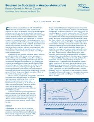
In East and Southern Africa (ESA), it has been shown that, despite the success of
export horticulture in some countries, and the great interest in replicating this in many
countries, domestic and regional systems will contribute most to total growth in demand
over at least the next 20 years. In addition, though supermarkets will continue to grow on
1

the continent, the broad consensus is now that their take over of market share will be
much slower than was anticipated by some, leaving the so-called “traditional” sector as
the dominant marketing channel for fresh produce for many years to come (Humphrey
2007, Traill 2006, Minten 2008, Tschirley et al. 2010).
There are many possibilities that horticulture commercialization offers to
smallholder farmers, however there are also many constraints smaller farmers face in
order to take advantage of these opportunities. The value that can be gained from
horticultural sales per unit of land is far greater than for widely marketable food crops
and even for cash crops such as cotton and tobacco. 1 This very high production value per
unit land area makes horticulture particularly attractive for land-constrained farmers --
who are the most likely to be poor. Since women frequently own the smallest plots, the
ability to capitalize on horticultural production might also have the benefit of off-setting
gender disparities in land access by enabling women to work their way out of poverty
through agriculture. The fact that product can be sold from a single horticultural field
multiple times over several weeks or months also provides built-in price risk management
opportunities that typical staple or cash crops do not offer. However, some of the risks of
horticultural marketing include (a) greater risk of losing one’s crop to pest or disease, (b)
high cost of inputs (fertilizer and pesticides) for a successful harvest, (c) very high price
variability, and (d) higher post-harvest perishability than other crops that are more easily
stored or can travel further distances to a market without spoiling.
1 See Appendix A for a comparison of crop value and input costs in Zambia, performed
by Chapoto et al. (forthcoming), which clearly illustrates the relative gross margins
between maize, cotton and horticultural crops.
2

The question then emerges of what type of smallholder farmer is able to
successfully exploit the opportunities provided by horticultural marketing, and whether
these farmers look different from those able to successfully exploit marketing
opportunities for other crops. Two recent analyses of the determinants of marketing
behavior of Mozambican smallholder farmers highlight the importance of personal
household characteristics and private assets in driving households’ ability to participate in
markets (Boughton, et al. 2007, Mather, Boughton and Jayne 2011) . These and other
analyses are reviewed in chapter three. In this thesis, these two papers are built upon and
extended by (a) examining a new crop group – fresh produce – that few if any authors
have yet examined, and (b) testing an enhanced number of variables, especially new
variables related to household location-specific characteristics. Given the differing
characteristics of fresh produce compared to most other food staple crops and cash crops,
explained above, it is hypothesized that the determinants of fresh produce marketing will
differ from those of these other crops in the following ways:
Land holdings will be substantially less important in explaining market
participation, though it may remain important in explaining the value of sales;
Controlling for land-holdings, a household’s being female-headed will continue to
have a negative impact on market participation and on the value of sales. This
impact is, however, likely to be the result of other factors correlated with having a
female household head that may not be perfectly controlled for in the analysis,
such as ownership of productive assets and access to capital;
3

Yet, because female-headed households are widely found to possess less land than
male-headed households, findings overall will suggest that fresh produce provides
opportunities to female-headed households that other crops do not;
Measures of household education may be more important than for other crops,
given the input- and knowledge-intensive nature of fresh produce production;
Location-specific factors will be more important in explaining fresh produce
market participation and value of sales. This will manifest itself in two ways: a
greater need for close proximity to (a) urban areas and good roads due to the high
perishability of fresh produce, and (b) bodies of water to support irrigation during
the cool-dry season, which is when pest pressure is least pronounced for these
crops;
This thesis proceeds as follows. Chapter two provides detail on the data sets used,
then present a descriptive survey of fresh produce and maize production and markets in
Mozambique over the last decade. Chapter three presents an econometric approach to
help profile successful maize and fresh produce sellers and the results of this model, and
implications of the study are summarized in conclusion (chapter four).
4

Chapter 2: Fresh Produce and Maize: A Descriptive Overview of Demand and
Supply in Mozambique
This chapter begins by describing the data used in this study, continues by
contextualizing this paper’s topic within the ESA setting of population growth, rising
urban per capita incomes and the effects of these on the demand for fruit, vegetables and
maize. The succeeding sections then elaborate on the specific empirical record of the
production and market activity of Mozambican commercialized sellers of fresh produce
and maize, in taking advantage of the opportunities this local increasing demand offers.
2.1 Description of the Data
This section outlines the sources of data used in this paper, starting with the
primary Mozambique survey data used in the empirical portions of this study, followed
by a description of the supplemental datasets drawn upon in the introductory section 2.2,
and ends with a section describing the spatial data used in the creation of five location–
specific variables used in the descriptive and econometric analyses of rural Mozambican
households found in sections 2.3 and 3.2 - 3.5..
2.1.1 Rural household survey data
Michigan State University has assisted in the collection of nationally
representative rural household survey data in Mozambique called the TIA (short for the
Portuguese Trabalho de Inquérito Agrícola) for many years. The data collected in years
2002 and 2005 constituted the most recent panel of this series. 4,908 households were
interviewed in 2002. The 2005 sample created a panel with 2002 and added 1,241
households (for a total sample size of 6,149) to be fully representative of conditions in
5

2005. Because of attrition, 4,104 of the 4,908 households interviewed in 2002 were able
to be re-interviewed in 2005. When presenting descriptive results in Chapter 2, the full
2005 data set is used. The econometric analysis presented in chapter three uses only the
panel households. As of this writing, the most recent year in which TIA data was
collected was 2008. Descriptive statistics using this most recent information are
therefore also used in the descriptive section of this paper, noting the relevant year.
Survey weights were applied according to the stratified sampling design of the survey in
the case of each year’s data for all computed statistics in this paper.
The data collected by the TIA includes household agricultural information on
cultivation practices, production, area and ownership of fields, sales, receipt of
agricultural price information, and prices at which sales occur for total value estimates
among a large variety of crops. In addition to this information, a rich set of household
and community level questions which are used to form variables in this analysis includes
information on the gender, age, illness, death, education level, and farmer association
membership of household head; family composition in terms of gender, ages,
consumption, occupation, and income of household members; and the degree to which
each community is affected by flood, drought, crop or livestock disease in the given year,
and the community’s proximity to primary natural water sources. 2
2 Data may be requested from Directorate of Economics, Ministry of Agriculture,
Mozambique. The author can refer interested parties to MSU personnel that can facilitate
such a request.
6

2.1.2 Supplemental Data
Income elasticities data from USDA: The Economic Research Service of USDA
estimated income elasticities of demand for a variety of food groups over 127 countries,
using national household expenditure survey data (see “International Food Consumption
Patterns: Income elasticity for food subgroups,” found at
http://www.ers.usda.gov/data/internationalfooddemand). This data is used to
demonstrate the expected magnitude and continued rise in demand for higher valued
crops, including fresh produce.
Population Information from the World Bank: The World Bank has estimates of
a variety of population statistics over the past 50 years for every country in the world.
This study uses their data on population growth, urban share of population growth and
urban population as a percentage of total population growth. These data can be found via
their databank link at the website http://data.worldbank.org/topic/urban-development.
2.1.3. Spatial Data
This study uses a number of spatial variables created using the latitude and
longitude coordinates of each of the 647 TIA villages. These coordinates were not
always recorded very precisely in the original questionnaire. To resolve this problem, I
use a list of over 10,000 village names in Mozambique and their accurate GIS latitude
and longitude coordinates to reassign these verified coordinate points to the villages in
the TIA, where possible. Of 647 villages, 236 are matched directly by name, 182 are
matched after comparing the TIA names with the list of over 10,000 names and assigning
7

matches where appropriate 3 and 229 are not able to be matched at all. In this latter case
the original TIA coordinate data is used. When projected within ESRI’s ArcMap10, 36
of the 647 villages are found to lie outside the national boundaries of Mozambique – all
36 are cases in which the original TIA coordinates were used and no match by village
name to a more accurate coordinate point was made. These village-cases are eliminated
from the map for the ensuing village variable creation, and their households are assigned
the village-average variable values for the district in which they lie.
The village level variables created with these coordinate points (later assigned to
all households within each respective village) include the following:
A. Average population density within a 10 km radius of the village. I generate this
variable using the geoprocessing tools buffer, clip, and the “zonal statistics as table”
feature within ArcMap10. The data used to create this variable are the United Nations’
2005 estimates given in population density grids of persons/square kilometer, urban
extents, and “urban points”/settlement points, obtained from the Global Rural-Urban
Mapping Project (GRUMP), all of which can be obtained from the website
http://sedac.ciesin.columbia.edu/gpw/global.jsp.
B. Average elevation within a 5 km radius of the village. I generate this variable
in a similar way as the population density variable. It uses v4.1 of the 90m digital
elevation data collected by the Shuttle Radar Topography Mission (SRTM), originally
produced by NASA and obtained from the Consultative Group on International
Agricultural Research - Consortium for Spatial Information (CGIAR-CSI). These can be
3
The author thanks Ellen Payongayong and David Tschirley for their help in verifying
the accuracy of these matches.
8

downloaded in very large grid-by-grid files from the website
http://srtm.csi.cgiar.org/SELECTION/inputCoord.asp.
C. A land cover “irrigation potential” dummy variable. The 2000 Global Land
Cover database produced by the Global Vegetation Monitoring Unit (a smaller
component of the Global Environment Monitoring Unit) of the European Commission’s
Joint Research Centre contains 24 global land classifications. I use these data to establish
whether a household resided within 1 km from a river or lake, within a swamp area
(forest or bush/grass land) or was given the land cover classification of “irrigated
cropland.” This data can be obtained from the website
http://bioval.jrc.ec.europa.eu/products/glc2000/products.php.
D. A variable for the total kilometers of primary or secondary road surface is
created at the district level using Africa-wide Michelin road data which is not available
for free online. 4 Road data obtained from the Digital Chart of the World also is used to
supplement this road data within the borders of Mozambique. This data is free and can
be downloaded from the website http://www.diva-gis.org/datadown.
E. Hours in travel time to the nearest town or city of 10,000 inhabitants or more is
generated using the “cost distance” function in ESRI’s ArcInfo10 Workstation.
Parameters specifying the length of time it would take an individual to travel along roads
of various qualities, or off-road, given land cover and elevation considerations (slope
impedance values and speed of travel were assigned given assumptions about travel by
foot, bike or car for example) are all incorporated in this raster analytic environment
4 These data were obtained from Jordan Chamberlin who had used them previously in
several versions of cost-distance variable creation (see E in this section) in ESA countries
while working for the International Food Policy Research Institute.
9

combining the elevation, land cover and roads data described above to calculate the
number of hours to a center of population density greater than 10,000, using the GRUMP
population data described above. The only data I use in the creation of this variable in
addition to those described in A-D above are administrative/political country boundaries
for which a general 30 minute delay was added in terms of added time to traverse. This
is relevant for villages close to the border of the country who may be selling across the
border. These Global Administrative Unit Layer (GAUL) maps are available through the
Food and Agriculture Organization of the United Nations (FAO) and can be found at the
website
http://www.fao.org/geonetwork/srv/en/metadata.show?currTab=simple&id=12691 or
from MSU’s Food Security GIS Resources Website:
http://www.aec.msu.edu/fs2/gis/boundaries.html. More information on the creation of
this variable can be found in Appendix B. 5
5 The author thanks Jordan Chamberlin and Steven Longabaugh for their help and the
various sessions held together to learn the process of cost-distance variable creation using
ESRI’s ArcMap10.
10

2.2 Strong Prospects for Fresh Produce Growth
The population in Sub-Saharan Africa has tripled over the past 50 years, starting
at a little over 200,000,000 in 1960, and surpassing 850,000,000 by 2010 (World Bank).
Figure 1 shows this increase in the form of an index, base year 1960 population = 100,
for Mozambique and Sub-Saharan Africa as a whole. Moreover, urban population as a
percentage of total population is also rapidly increasing. In Mozambique, this percentage
has grown from 5% in 1960 to close to 40% in 2010 (Figures 2 and 3). Per capita income
of these increasingly urban habitants is also projected to increase dramatically as
industries continue to grow and develop, providing manufacturing job income to many
who are leaving their rural homes for the higher wages provided in these sectors.
Figure 1: Population Growth, Index Base Year 1960
400
350
300
250
200
150
100
50
0
Source: World Bank
1960
1965
1970
1975
1980
1985
1990
1995
2000
2005
2010
Year
Mozambique Sub-Saharan Africa
Note: For interpretation of the references to color in this and all other figures, maps or
tables, the reader is referred to the electronic version of this thesis.
11

Figure 2: Urban Share of Population Growth in Mozambique, 1960-2010
Population
25,000,000
20,000,000
15,000,000
10,000,000
5,000,000
Source of Data: World Bank
0
1960
1966
1972
12
1978
1984
Year
1990
1996
2002
2008
Total Population Urban Population
Figure 3: Urban Population as Percentage of Total in Mozambique
% of Total Population
50
40
30
20
10
0
Source of Data: World Bank
1960
1965
1970
1975
1980
1985
Year
1990
1995
2000
2005
2010

Growth in income and urban population shares have led to a situation where
expenditure on fresh produce, meat and dairy products is rising more rapidly across
developing countries than anywhere in the world. In the long-run, as incomes rise, the
income elasticity of demand for food falls. This can be represented by comparing the
relative income elasticities for a variety of food groups in Mozambique to a higher-
income country such as the United States, as is visually depicted in figure 4. The income
elasticity for a crop represents the percentage change in consumption for a 1% rise in
income. In every food category, the income elasticity of demand in the U.S. is less than
the respective elasticity in Mozambique, meaning that if those in the U.S. received 10%
more in income, their spending on food would rise less in percentage terms than the
respective expenditures of an average African. The reason for this is intuitive: as
incomes rise, proportionately less of one’s salary needs to be spent on items such as food,
and can be designated to functions or items that are less vital or necessary to life: this is
Engel’s Law. Bennett’s Law represents a similar and related concept which is also
evidenced by the elasticity patterns in figure 4: as incomes rise, the types of foods that are
consumed tend to transition from cheaper and often less nutritionally-rich goods such as
grains, to “luxury” food items such as dairy, meat, and fresh produce. All of the latter
food types have higher income elasticities than the elasticity for cereal, which is actually
negative in the case of the U.S. Given these two economic principles (Engel’s Law and
Bennett’s Law) at work in lower-income developing countries such as Mozambique,
expenditure on fresh produce is rising much more rapidly with increasing incomes in
these countries than it is in more developed countries such as Europe and the U.S., and
will continue to do so until incomes across the region are much higher.
13

Figure 4: Income Elasticity of Demand for Several Food Groups: Mozambique and the
United States
Income Elasticity
2.000
1.500
1.000
0.500
0.000
-0.500
Cereals Meats Fish Dairy
Mozambique 0.600 0.815 0.703 0.843 0.611 0.671 1.745 1.346
United States -0.085 0.343 0.260 0.354 -0.001 0.210 0.438 0.424
Food SubGroup
Source of Data: USDA, Economic Research Service
14
Oils/
Fats
Fruits Other Bev./To
bacco
Figure 4 shows that the elasticity of fruit consumption in Mozambique is
0.67,meaning that for every 1% rise in income, expenditure on fresh produce in
Mozambique rises by 0.67%. In the U.S., a 1% increase in income would only increase
fruit consumption by 0.21%. The income elasticity of demand for fruit in Mozambique is
greater than that for maize in Mozambique, at .60, and approaches the elasticity values of
meat (.81), fish (.70) and dairy (.84). All of these indicators show that fresh produce, and
fruit in particular, present strong prospects for growth as incomes rise in ESA, and this
growth represents a major opportunity for domestic and regional supply (local farmers) to
meet the burgeoning local demand.

2.3 Empirical Patterns
2.3.1 Which farmers are exploiting the opportunities presented by horticultural
crops?
According to the national agricultural survey of Mozambique in 2008, 78% of all
farming households in the country produced maize, 64% produced fruit, and 36%
produced vegetables. Among these same crops, 16% of households sold maize, 13% sold
fruit, and 8% sold vegetables (Figure 5).
Figure 5: Market Participation Decisions among Maize, Fruit and Vegetable Farmers
70.0%
60.0%
50.0%
40.0%
30.0%
20.0%
10.0%
0.0%
Source of Data: TIA 2008
Did not
produce
Produced,
did not sell
15
Produced
and sold
Maize
Fruit
Vegetables

Despite some government support to maize sellers 6 and private contracting
support for cash crop sales, the percentage of those producing or selling either fruits or
vegetables as a group were greater than those who sold maize (18% compared to 16%),
or cash crops (information not reported here). The following tables report these numbers
and show a number of household characteristics by each of these crop types (fruit in table
1, vegetables in table 2, all fresh produce – fruits and vegetables - in table 3, and maize in
table 4) in terms of whether the household produced each crop, sold each crop, and at
what quintile of sales value the household sold for each crops’ selling group component.
6 Government support for maize commercialization in Mozambique has included some
extension assistance, seed provision, and recently, a pilot fertilizer voucher scheme,
although in comparison with some of its neighboring countries, government assistance in
Mozambique has been substantially less.
16

Table 1: Household characteristics by fresh produce production and sales behavior – Fruit
Group
Share
of all
HH value of
fruit sales
(US$)
HHs Mean Median
Group’s
share of
total
national
fruit
sales
HH income per
capita (US $)
Mean Median
17
Share of
fruit
sales in
total
HH
income
%
female
headed
Years formal
education of
HH head
Total land
holdings (ha)
HHs Mean Median Mean Median
Did not produce 35.7% $123 $56 25.2% 2.8 2.0 1.5 1.2
Produced but did not sell 51.8% $175 $80 24.7% 3.1 3.0 1.7 1.3
All fruit sellers 12.5% $32 $7 100% $183 $97 5.4% 18.3% 3.1 3.0 2.1 1.6
Quintile 1 (sold the least) 2.6% $1 $1 0.8% $138 $71 0.1% 23.1% 2.3 2.0 1.6 1.3
Quintile 2 2.6% $4 $3 2.3% $133 $77 0.7% 19.5% 2.9 3.0 1.7 1.4
Quintile 3 2.3% $8 $7 4.3% $158 $101 1.6% 15.7% 3.3 4.0 1.8 1.6
Quintile 4 2.5% $17 $15 10.5% $188 $110 4.3% 18.6% 3.0 3.0 2.4 1.7
Quintile 5 (sold the most) 2.5% $135 $69 82.1% $301 $153 17.5% 14.0% 3.8 4.0 3.0 2.5
Source of Data: TIA 2008

Table 2. Household characteristics by fresh produce production and sales behavior – Vegetables
Group
Share
of all
HH value of
vegetable
sales (US$)
HHs Mea
n Median
Group’s
share of
total
national
veg.
sales
HH income per
capita (US $)
Mean Median
18
Share of
vegetable
sales in
total HH
income
%
female
headed
HHs
Years formal
education of
HH head
Total land
holdings (ha)
Mean Median Mean Median
Did not produce 63.8% $150 $67 24.8% 2.9 3.0 1.5 1.2
Produced but did not sell 28.4% $165 $83 24.7% 2.9 3.0 1.9 1.4
All vegetable sellers 7.8% $65 $20 100% $193 $102 8.4% 16.4% 3.4 3.0 2.4 1.9
Quintile 1 (sold the least) 1.9% $2 $2 0.9% $118 $85 1.8% 21.2% 3.3 4.0 1.8 1.6
Quintile 2 1.3% $7 $7 1.8% $185 $73 2.4% 17.7% 3.4 3.0 2.2 1.6
Quintile 3 1.6% $20 $21 6.2% $157 $110 4.9% 16.2% 3.1 3.0 2.5 2.0
Quintile 4 1.5% $48 $45 14.2% $197 $124 10.9% 19.8% 3.2 3.0 2.1 1.9
Quintile 5 (sold the most) 1.5% $252 $165 76.9% $327 $176 22.7% 6.2% 4.1 4.0 3.3 2.6
Source of Data: TIA 2008

Table 3. Household characteristics by fresh produce production and sales behavior - All fresh produce
Group
Share
of all
HH value of
fresh produce
sales (US$)
HHs Mean Median
Group’s
share of
total
national
fresh
produce
sales
HH income per
capita (US $)
Mean Median
19
Share of
fresh
produce
sales in
total HH
income
%
female
headed
Years formal
education of HH
head
Total land
holdings (ha)
HHs Mean Median Mean Median
Did not produce 24.9% $119 $54 25.7% 2.8 2.0 1.4 1.1
Produced but did not sell 56.9% $168 $75 25.4% 3.0 3.0 1.7 1.3
All fresh produce sellers 18.2% $50 $10 100.0% $176 $94 7.3% 17.8% 3.1 3.0 2.1 1.7
Quintile 1 (sold the least) 3.8% $1 $1 0.6% $112 $75 1.3% 22.0% 2.3 2.0 1.5 1.3
Quintile 2 3.7% $5 $4 2.0% $144 $78 2.0% 20.8% 2.8 3.0 1.7 1.3
Quintile 3 3.6% $11 $11 4.4% $154 $90 3.9% 21.2% 3.4 3.0 2.1 1.6
Quintile 4 3.6% $31 $29 12.4% $196 $131 7.5% 14.3% 3.1 3.0 2.4 2.0
Quintile 5 (sold the most) 3.6% $203 $114 80.6% $277 $140 22.2% 10.3% 4.0 4.0 3.0 2.5
Source of Data: TIA 2008

Table 4. Household characteristics by fresh produce production and sales behavior – Maize
Group
Share of
all HHs
HH value of
maize sales
(US$)
Mean Median
Group’s
share of
total
national
maize
sales
HH income per
capita (US $)
Mean Median
20
Share of
maize
sales in
total
HH
income
%
female
headed
Years formal
education of
HH head
Total land
holdings (ha)
HHs Mean Median Mean Median
Did not produce 21.7% $152 $60 6.8% 28.5% 2.9 2.0 1.0 0.8
Produced but did not sell 62.1% $153 $73 25.8% 25.7% 2.9 3.0 1.7 1.4
All maize sellers 16.2% $89 $28 100.0% $181 $96 34.3% 12.1% 3.2 3.0 2.4 1.9
Quintile 1 (sold the least) 3.4% $5 $6 1.3% $105 $68 25.5% 22.4% 2.3 2.0 1.6 1.3
Quintile 2 3.2% $14 $12 3.0% $139 $92 26.8% 16.2% 2.9 3.0 2.2 1.8
Quintile 3 3.2% $28 $28 6.2% $122 $83 34.9% 8.2% 3.2 3.0 2.0 1.7
Quintile 4 3.3% $58 $56 12.9% $190 $105 36.7% 5.7% 3.6 3.0 2.6 2.1
Quintile 5 (sold the most) 3.2% $345 $148 76.6% $354 $198 47.8% 7.9% 3.9 4.0 3.8 3.1
Source of Data: TIA 2008

The first thing to notice about these tables (1-4) is the very high concentration of
sales value. The top fifth of sellers in every category earns 80% or more of the
smallholder share of national value obtained from these crops’ sales. The bottom 60% of
sellers account for only an average of 7% of the value for fresh fruit or vegetable sales,
and these 60% do not earn more than an average $10-20 at best over the given survey
year, with values higher for vegetable sales than for fruit. The bottom 60% of maize
sellers has average sales ranging up to $20-30 in a year. Also among the commercialized
top selling quintile, maize sellers are doing quite a bit better than fresh produce sellers,
with average sales $30-145 higher than average sales for fresh fruits and vegetables
(FFV). A cross-country comparison of the high concentration of sellers between
Mozambique, Zambia and Kenya can be found in Figure 6, showing nearly identical
concentration in each country. Figure 7 shows concentration across all three crop
categories in Mozambique, demonstrating that all these crops’ marketing pattern is
similarly concentrated.
21

Figure 6: Share of fresh produce sales by quintile of sale value: Zambia, Mozambique,
and Kenya
Share of national sales
0.90
0.80
0.70
0.60
0.50
0.40
0.30
0.20
0.10
0.00
Quintile 1
(sold the
least)
Quintile 2 Quintile 3 Quintile 4 Quintile 5
(Sold the
most)
Quintiles of FFV Sales
Source: Tschirley (2010). Mozambique data is taken from the TIA 2008
22
Mozambique
Zambia
Kenya

Figure 7: Share of sales by quintile of sales value: Fruit, Vegetables, Fresh Produce
(Fruit and Vegetables Combined) and Maize
Share of National Sales
90.00%
80.00%
70.00%
60.00%
50.00%
40.00%
30.00%
20.00%
10.00%
0.00%
Quintile 1
(sold the
least)
Source of Data: TIA 2008
Quintile 2 Quintile 3 Quintile 4 Quintile 5
(sold the
most)
Quintiles of FFV Sales
23
Fruit
Vegetables
All Fresh Produce
Maize
Even the households that sell in the lowest quintile of fruit sale value have higher
mean and median incomes per capita than those who did not sell fruit. This is not true of
vegetable sellers, where households in the lowest quintile of sales have lower mean and
median incomes per capita than non-sellers, similar to the distribution of maize sellers.
Households who produce but do not sell retain higher average and median incomes per
capita than those who do not produce among all three crops. These findings suggest that
the production of maize, fruit or vegetables is indicative of a higher standard of living,
but only in the case of selling fruit are sellers universally found at a higher income status.
Households in the bottom quintiles of vegetable or maize sale values evidence lower
household income than those who do not sell at all.
Among the top quintile of maize sellers, half of the household’s income on
average is accounted for by maize sales. The percentage of total income accounted for by

FFV sales is less, 22% of total income as compared to 46% of total income for maize.
This percentage is driven by the higher values of vegetable sales, while top fruit sellers’
fruit incomes only account for an average 17% of fruit-selling households’ total income.
This indicates that many farming families are either growing higher-value crops in
addition to maize or fresh produce, or have income from off-farm activity, remittances or
pensions.
Between maize and FFV-sellers, female-headedness looks strikingly similar, with
rapidly falling shares of female-headed households as one moves from the lowest quintile
of sale value to the highest. There are also few differences between landholding or
educational level between FFV sellers and maize sellers. Landholding ranges from 1.8 to
3.3 hectares for maize-sellers and 1.6 to 3.0 hectares for FFV sellers. Household head
education levels range from 3.3 to 4.1 among maize-sellers and 2.3 to 3.8 among FFV-
sellers, despite the higher knowledge or “know-how” requirements of producing fresh
produce. These trends will be explored in greater detail in latter portions of this thesis.
This next section will first consider the question of how many fresh produce sellers are
also maize sellers, and vice versa.
24

2.3.2 Do selling households sell one crop only, or multiple crops, and how does this
affect their performance?
According to data from the TIA 2005, 2/3rds of farmers that sell fresh produce do
not sell maize or cash crops 7 – they specialize in fresh produce sales. These results
closely resemble those generated from the TIA 2008, lending robustness to the
percentages found (Tschirley 2011). Clearly, some farmers are finding fresh produce
generates income they are not making from sales of other crops, especially given that
farmers make these choices to only sell fresh produce despite producing either maize or
cash crops on their fields they choose not to sell. These patterns can be seen in the
figures below for production behavior (Figure 8) and market behavior (Figure 9) of four
mutually exclusive groups of fresh produce sellers: (a) those that sell/produce fresh
produce, maize and cash crops, (b) those that sell/produce fresh produce and cash crops
but not maize, (c) those that sell/produce fresh produce and maize but not cash crops, and
(d) those that only sell/produce fresh produce.
7 The cash crops group includes cotton, tobacco, sesame, sunflower, coffee, tea, and
paprika.
25

Figure 8: Production Behavior of Fresh Produce Sellers
Source of Data: TIA 2005
15%
26
18%
1%
66%
All three crops: maize and cash crops and fresh
produce
Cash crops and fresh produce but not maize
Maize and fresh produce but not cash crops
Only fresh produce

Figure 9: Market Behavior of Fresh Produce Sellers
Source of Data: TIA 2005
64%
27
6% 8%
22%
All three crops: maize and cash crops and fresh
produce
Cash crops and fresh produce but not maize
Maize and fresh produce but not cash crops
Only fresh produce
The following two depictions (figures 10 and 11) take a closer look at fruit and
vegetable sellers separately as they compare to maize sellers by proportionately
displaying the number of farmers who choose to produce and sell fruit, vegetables, or
maize, and how many of these also produce or sell two or all three of these together on
their land. These graphs are called Euler diagrams, and they are similar to Venn
diagrams except they keep quantitative spatial relationships between three concentric
“circles” intact.

Figure 10: Maize, Fruit and Vegetable Production Behavior among Sellers of these
Crops 8
Source of Data: TIA 2005
8 These diagrams are generated using the “Draw Euler” free software created by Stirling
Chow -- senior java software developer for AlarmPoint Systems Incorporated. The
author thanks Francis Smart for his help in creating them.
28

Figure 11: Maize, Fruit and Vegetable Market Behavior
Source of Data: TIA 2005
It can be observed from these graphs that more farmers are selling fruit than
vegetables, with fruit looking very similar to maize in terms of the number of farmers
specializing in maize and fruit production and sales. Similar to what was found in the
graphs looking at fresh produce sales as a whole above, 63% of those who sell fruit, only
sell fruit, 45% of those who sell vegetables only sell vegetables, and the percentage of
those who only sell maize among the maize sellers is only slightly higher than that of
fruit – at 66%. This shows that production is much more diversified than sales,
29

suggesting that different factors determine choice of commodity to sell than determine
choice of commodity to produce.
Vegetables also seem rarely to be grown without another crop, and a mere 1% of
farmers only produce vegetables. Given that the average value of vegetable sales is
greater than the average value of fruit sales, the lack of specialization in vegetable sales
probably relates to the fact that vegetables are very risky to grow, and farmers are
diversifying their risk by growing other crops. It is also not certain that the net benefit of
selling vegetables is greater than that of selling fruit.
Between maize, fruit and vegetables, farmers most frequently specialize in maize
sales (36% of all FFV or maize sellers sold only maize) with fruit following close behind
(32% only sold fruit). Farmers least frequently specialize in vegetable sales (10% of all
fruit, vegetable or maize sellers). Proportionally, farmers who sell only maize are least
likely to grow the other two crops on their fields than farmers who sell only fruit or only
vegetables (72% of the group that specializes in maize sales also grows fruit or
vegetables, compared to 81% that specializes in fruit sales that also grows maize or
vegetables and 90% that specializes in vegetable sales, that also grows maize or fruit.
This information is summarized in figure 12.
30

Figure 12: Are Specialized Sellers Diversified Growers?
Percent
40
35
30
25
20
15
10
5
0
Source of Data: TIA 2005
Maize, Fruit and Vegetable Sellers: Are
Specialized Sellers Diversified Growers?
Maize Fruit Vegetables
31
Percent of total sellers
that only sold one of
the three: Maize, Fruit
or Vegetables
Percent of total sellers
that also harvested
one or more of the
other two crop types
A Euler diagram is also used to depict, among fruit, vegetable and maize sellers,
which groups earn the most for their sales out of the total value of all maize, fruit and
vegetable sales in Figure 13. This graph makes it especially apparent that whereas fewer
farmers commercialize their vegetable production rather than their fruit production, the
value obtained from selling vegetables is far greater than the value obtained from fruit:
fruit-only sellers (32% of all maize, fruit and vegetable sellers) only account for 8% of
the total sales value, whereas vegetable-only sellers (10% of all sellers) account for 12%
of the total value, and 23% of the total value of sales are obtained by farmers who grew
both maize and vegetables. Between FFV and maize groups respectively, 31% of total
sale value is obtained by farmers who specialize in only selling maize (no fruit or
vegetables), and 26% of the value is obtained by farmers who specialize in only selling
fruit, vegetables or both fruits and vegetables (no maize). This would indicate that the
barriers facing vegetable sellers differ from those faced by fruit sellers, and the

challenges for vegetable sales pose constraints less farmers have overcome than those
who have overcome the barriers to participate in commercialized status of their fruit (or
maize) production.
Figure 13: Total Value Obtained from Fruit, Vegetable and Maize Sales
Source of Data: TIA 2005
32

Figure 14: Mean and Median Annual Sale Values of Seven Crop Groupings
Sale Value in USD
$140
$120
$100
$80
$60
$40
$20
$-
Maize, fruit and vegetables
Maize and fruit, not vegetables
Source of Data: TIA 2005
Mean and Median Annual Sale Value
Maize and vegetables, not fruit
33
Only Maize
Only Fruit
Only Vegetables
Fruit and Vegetables, not maize
Mean Total Sale Value Median Total Sale Value
Reflected in Figure 14, the mean value of sales over all crops (maize, cash crops,
fresh produce) is lowest among the groups which sell only one crop. The mean value of
sales is highest for farmers who sold fruit and vegetables together without maize, and the
median value of sales is highest for farmers who sell fruit, vegetables and maize. These
high market values give evidence of the existing (and growing) local demand for fruit and
vegetables in Mozambique.

2.3.3 Persistence of Successful Fresh Produce or Maize Marketing
It was noted from section 2.3.1 that agricultural sales are highly concentrated in
Mozambique. It was then shown in section 2.3.2 that many FFV sellers only sell fruit or
vegetables, therefore cash income is being achieved by farmers in horticulture that is not
being found by selling other crops. It is also worthy to note that of those that are in the
top sales quintile of fresh produce or maize, very few remain in the top sales quintile over
the course of time.
Between the two panel years of the TIA (2002 and 2005), only 3.17% of FFV
sellers are in the top quintile of sellers in both years, and similarly among maize sellers,
only 2.9% of sellers remain in the top quintile. Tables 5 and 6 take a closer look at the
4,104 farmers who were interviewed in both years of the TIA survey in regards to their
marketing behavior, to better understand the proportions of farmers who sell in both
years, those who are persistent top-sellers in both years, and the spatial distribution of
these sellers. Tables 7 and 8 explore household characteristic differences between these
groups to help understand if top sellers in maize look different from top sellers in fresh
produce, as well as what distinguishes each top-selling group from the other farmers who
sold.
Table 5. The percentage of households selling FFV and maize in each of the panel
years of the TIA data used
% of
HHs
Selling
Nationally Southern Region Central Region Northern Region
FFV Maize FFV Maize FFV Maize FFV Maize
2002 31.2% 21.2% 31.6% 4.7% 42.4% 25.4% 27.4% 24.8%
2005 22.7% 17.8% 20.2% 2.7% 23.2% 23.4% 23.2% 20.5%
34

Table 6. Top-Selling Households by Region of Mozambique
Region FFV Maize
----- % of HHs in top selling tercile during both years -----
Southern 10.0 4.2
Central 10.1 5.2
Northern 2.5 4.9
These tables show that 17-31% of all farmers in both panel years sell either fresh
produce or maize in either 2002 or 2005, with lower percentages of those selling in both
crop categories in 2005 compared to 2002, due to a serious drought during 2005. Most
maize sales are accounted for in the central and northern regions, whereas FFV sellers as
a group are fairly evenly distributed across the country. Of households in the top third, or
tercile, of either FFV or maize sales in both years, 5.46% of FFV sellers remain in the top
selling group over the two years, and 4.97% of maize sellers remain in the top selling
group over the two years. The percentage of top FFV sellers in both years is
concentrated in the southern and central regions with both above 10% of the persistent
top sellers, and only 2.43% in the northern region. The percentage of top maize sellers
by region is fairly consistent across the country’s regions, at 4.2-5.2% of sellers, even in
the southern region where only 2-5% of farmers participate in maize marketing. These
results generally show that there is only an incipient group of established commercialized
FFV providers in Mozambique, and a wide window exists for market improvement.
35

Descriptive statistics for a variety of household-level characteristics are compared
between (a) top selling FFV and maize groups (b) top selling FFV and non-top selling
FFV groups, and (c) top selling maize and non-top selling maize groups. Table 7
displays percentages of discrete variables, table 8 displays means and medians of
continuous variables, and the results are interpreted in terms of two congruent sets (one
set for the discrete variables, and the other for the continuous variables) of five areas:
market access, assets, agro-ecological factors, price/wealth effects, and demographic
characteristics. The rationale for this grouping is described in the following chapter. In
the remainder of this section, the term “top-selling” refers only to the group which sells in
the top tercile of sale values among all sellers in both years of the panel dataset. 9
9 I move to terciles from this point forward for a more meaningful analysis of household
characteristics between groups in the next section, due to the fact that the numbers of
households in top sales quintiles during both years is so small (about 3%-4% of sellers,
meaning less than 1% of the total population).
36

Table 7. Comparison of Fresh Produce and Maize Persistent Top-Sellers, Discrete
Variables
FFV
Persist
ent
Top
Sellers
(5.5%)
FFV
Non-
Top
Sellers
(94.5%)
37
Maize
Persist
ent
Top
Sellers
(5.0%)
Maize
Non-
Top
Sellers
(95.0%)
Top
vs
Top
Top
vs
Nontop
FFV
Price Information 38% 38% 62% 42% ** **
Association Member 18% 5% 4% 4% ** ***
Manual irrigation 40% 14% 10% 9% *** ***
Mech/Grav Irrigation 12% 1% 1% 1% *** **
Irrigat’n potent'l area 3% 4% 0% 3% ** ***
Close to river/lake 39% 38% 64% 46% *** **
HH salaried worker 6% 5% 11% 4%
HH-head is female 13% 21% 13% 20% *
Top vs
Nontop
Maize
Note: T-tests were used to determine whether the means between groups were
statistically different, and asterisks reflecting these tests are given in one of three columns
on the right side for each respective group comparison (p > 0.10*, p > .05**, p > .01***).

Market Access
One of the factors that differentiates maize top-sellers from maize not-top sellers
is receiving price information: 62% of top sellers report receiving price information,
whereas only 42% report receiving price information among not-top sellers. Market
information is generally limited to food staples, and is not available for fresh produce
items, however. The comparison between top-sellers and non-top sellers of FFV reflects
this in a lower percentage of FFV-selling farmers, only 38%, who report receiving price
information.
Assets
Important differences are found in regards to farmer association membership:
18% of the household heads among FFV top sellers are members of an association,
whereas non-top sellers have a rate of 5%. A slightly lower average of 4% of both top
maize sellers and non-top maize sellers participate in an association. Irrigation also
plays a role for fresh produce sellers in a way that does not affect maize sellers: 40% of
top FFV sellers reported using manual irrigation and 12% reported using mechanical or
gravity irrigation compared to only 10% and 1% reported by top-maize sellers
respectively. Not surprisingly, this variable is significantly different between top-FFV
sellers and non-top sellers, the latter of which have rates of 14% and 1% manual and
gravity/mechanical irrigation: only a fourth of their top-selling counterparts in each case.
38

Agro-Ecological Factors
A significantly greater percentage of households who sell in any FFV-selling
tercile is more often located in an “irrigation potential area” – those that are identified
with a land cover map as primarily lying in either an irrigated, watery or swampy area --
than households who sell maize, despite the very low prevalence of this variable across
all households. None of the top-selling maize sellers are recorded as lying in these areas,
however persistent top-sellers of maize have greatest access to or use of lake or river
water for community or agricultural use of all of the categories, at 64% compared to 46%
of farmers in the lower 2/3rds of maize sellers, and compared to 38-39% of fresh produce
sellers.
Price/Wealth Effects
Slightly higher percentages of both FFV and maize-selling households report
having a salaried worker in the household (6% compared to 5% for FFV and 11%
compared to 4% for maize). None of these differences across crop groups or within
groups are significant, however. This could be due to a dual effect: the additional income
can help invest in the household’s fields or reflect the amount of value that can be
obtained from these investments, as well as the amount of outside experience or
knowledge gained, but on the other hand, jobs off farm may take away from the labor
requirements of the farm, especially in the case of FFV. This ambiguity in itself, in this
way, may indicate both of these factors at play.
39

Table 8: Comparison of Fresh Produce and Maize Persistent Top-Sellers, Continuous Variables
FFV Persistent
Top Sellers
(5.5%)
FFV Non-Top
Sellers (94.5%)
40
Maize Persistent
Top Sellers
(5.0%)
Maize Non-Top
Sellers (95.0%)
Top
vs
Top 10
Var Name Median Mean Median Mean Median Mean Median Mean
Hours to town, 10K+ 3.3 4.8 5.5 7.0 6.5 8.6 6.3 7.9 *** ***
Km of district roads 21.2 22.8 22.6 24.1 31.0 29.1 24.7 27.0 ***
Population density 20.7 41.2 27.2 41.7 32.4 42.5 25.2 34.4
Adult max education 4.0 4.8 3.0 3.7 4.0 3.9 3.0 3.4 * ***
Number of fields 3.0 2.8 3.0 2.7 3.0 2.7 2.0 2.5
Land area in hectares 2.3 3.0 1.4 1.8 1.9 2.6 1.4 1.9 *** *
Other assets (1-6) 3.0 2.7 2.0 2.0 2.0 1.8 2.0 1.8 *** ***
No. fruit trees 4.0 4.6 3.0 3.1 2.0 2.7 2.0 2.1 *** ***
Elevation (100 m) 10.0 11.2 10.2 10.9 10.0 10.3 10.2 11.0 *** **
Expected drought days 1.2 1.5 0.6 1.0 0.6 0.8 0.5 0.8 *** ***
Age of HH-head 42.0 46.8 41.0 42.3 36.0 35.7 39.0 40.7 *** ** ***
HH consumption size 4.3 4.8 3.5 3.9 3.9 4.1 3.4 3.7 *** ***
10
T-tests compare means, not medians Asterisks reflecting these tests are given in one of three columns on the right side for each
respective group comparison (p > 0.10*, p > .05**, p > .01***).
Top
vs
Nontop
FFV
Top vs
Nontop
Maize

Demographic Characteristics
The percentage of female-headed households among top FFV and top maize
sellers is not significantly different, at 13% for both. FFV and maize non-top selling
categories also look surprisingly similar, both are headed by females 20-21% of the time.
Given that the smallest plots tend to be those governed by females, the opportunity for
fresh produce sales among these households would seem to be particularly great.
Female-headed households hold an average 1.2 hectares of land per household,
significantly differing from the average 1.8 hectares owned per male-headed household.
Summarizing the key patterns among the discrete variables discussed, receipt of
price information distinguishes top maize sellers from non-top maize sellers, access to
irrigation and farmer associations distinguishes top-FFV sellers both from top-maize
sellers and from their non-top counterparts, and top sellers of both crops are equally
likely to be headed by males.
I now turn to the continuous variables included in Table 8 in identifying other
distinguishing characteristics among the more and less successful fruit, vegetable and
maize sellers.
Market Access
Top-FFV sellers are distinguished from top-maize sellers in a significant way
through the number of hours in travel time to a town or city of greater than 10,000
inhabitants. The median distance in hours for top-FFV sellers is 3.3, and the median
distance for non-top FFV sellers is 5.5, a value that is still smaller than the median value
of top or non-top maize sellers, both of which fall between 6.3 and 6.5 hours. There is
41

also significantly more average road density in top-selling maize districts of household
residence than the comparative top-selling FFV group districts, by an average 63,500
kilometers of primary or secondary paved surface (standard deviation of 110,000 km).
Uncertain of what exactly lies behind the second of these two conclusions, the first is
quite clear and pronounced: both fruit and vegetables are highly perishable and thus
cannot travel far distances to a market of meaningful size at which sales would more
often occur. This characteristic both for fresh produce as a group compared to maize, as
well as successful and persistent top growing fresh produce suppliers indicates the vital
role of spatial positioning for a successful FFV-selling household, and some of the
potential constraints which farmers may face in otherwise selling their fruits and
vegetables compared to maize.
Asset Base
In terms of human capital/assets, top sellers in FFV have significantly higher
average maximum household adult years of education achieved than FFV non-top selling
households (4.8 compared to 3.7), while this relationship between maize top sellers and
non-top sellers is not significant. Top FFV-selling household adults also have
significantly more average maximum years than top maize-sellers (4.8 compared to 3.9
years for maize). Both of these results are expected for a knowledge/expertise intensive
group of crops, as fruit and vegetables are more susceptible to pests and weather both
during and after harvest, as compared to maize.
Top sellers of both maize and FFV have significantly larger areas of land than
their non-top selling counterparts by around one hectare (average 3.0 compared to 1.8 for
42

FFV, and 2.6 compared to 1.9 for maize). Interestingly, maize top sellers do not have
significantly more land than FFV top sellers, which is further evidence that small land-
holders have not yet really entered the top-selling horticulture groups yet. The number of
fields (around 3 on average) does not vary significantly across all the groups.
Other assets (a variable with a range of 1-6 for owning any of the following
assets: storage facility, good roof, good walls, latrine, lamp, table) make a much larger
difference for FFV sellers and do not make any difference among maize sellers. Top
FFV-sellers have an average of three compared to two of the six items recorded by top
maize sellers and non-top FFV sellers. And top-sellers in both crop categories
consistently have more farm and livestock asset value than their non-top selling
counterparts.
Not surprisingly, number of fruit trees is significantly higher for the successful
fresh produce sellers compared to both the non-top fresh produces sellers and the maize
top-sellers, with the median number of trees at 4, 3 and 2 for top FFV sellers, non-top
FFV sellers and any maize seller respectively.
Agro-Ecological Factors
The number of expected drought days by the household for the given year (a
description of how this variable was created can be found in the next chapter) is
significantly higher on average for top FFV sellers than for non-top FFV sellers, and
significantly higher for top FFV sellers than for top maize sellers. Since drought or less
rain is a good thing for vegetable production as long as a household has access to
irrigation, lower expected drought days in the year for top maize households makes
43

sense. Average elevation is higher for the top-selling fresh produce group compared to
the top selling maize group given the cooler areas in higher elevations where there are
less pest problems than in some of the more tropical conditions where maize farmers can
still do well. Nonetheless, the result on maize is somewhat counter-intuitive given that
mid-altitude elevations enhance hybrid maize expression. Maps depicting both rainfall
and elevation throughout the country to contextualize these findings can be found in
Appendix C.
Demographic Characteristics
Top FFV-selling household heads are significantly older than top maize-sellers by
an average of 10 years, and older than non-top FFV selling household heads by an
average of 4 years. This stands in contrast to top maize sellers who are significantly
younger than the non-top maize sellers by about 5 years on average. This is an
unexpected finding, and is reversed in the regression analysis of chapter three. These
results are further explored in section 3.6. Perhaps also related to age, top FFV sellers
have significantly larger household sizes in adult consumption equivalents than top maize
sellers. Top-FFV selling households also are significantly larger in consumption
equivalents than non-top FFV selling households, by about the same degree. It is
possible that the labor intensive requirements of fresh produce cultivation would be a
reason for both larger household sizes and older household heads, who may have greater
numbers of grown children working in the fields. There is no significant relationship
between top and non-top selling maize households in their household size.
44

Summarizing the key patterns, this section interpreting Table 8 finds that market
access in terms of fewer hours to reach a town of meaningful size, higher education levels
of an adult household member, level of overall assets and number of expected drought-
days are all significant in the case of top fresh produce sellers in comparison to non-top
FFV sellers and maize sellers. Greater land size characterizes both top-selling maize and
top-selling FFV households in comparison to their non-top selling counterparts, whereas
number of plots shows no significant difference among any selling group. FFV top-
sellers are found to succeed in higher elevations on average compared to maize-sellers,
and the top maize sellers succeed in even lower elevations, compared to their non-top
selling counterparts. Household head age and household size in consumption equivalents
also yields mixed results between FFV and maize sellers: younger is better for maize
sales, while older and larger is more common among successful fresh produce sellers,
indicating a possibly larger labor base for the intensive production practices of a thriving
fresh produce practice, and possibly the additional management practice gained with time
or experience of an older household head.
The next chapter introduces a modeling approach that will allow a closer look at
the effect of the variables already introduced and a number more, while controlling for
the effect of the others.
45

Chapter 3: Modeling smallholder fresh produce farmer market participation
decisions
This chapter first summarizes the market participation literature in Africa to
motivate the modeling approach used in this empirical analysis. It then presents the
chosen modeling approach in more detail, explains all chosen independent variables, and
presents estimation results, before closing with a discussion of the implications of this
study.
3.1 Summary of Market Participation Literature
Literature on market participation in ESA has well documented the importance to
household commercial decision processes of (1) the level of market development in the
environment facing the farmer, and (2) the farmer’s private asset holdings. Research on
both these areas can be traced to seminal contributions on smallholder market behavior
made by De Janvry et al. (1991). In the first area, much work has been devoted to
developing a better conceptualization and understanding of the effects of market access,
infrastructure and transaction costs as they affect household market decisions. Key
contributing authors in this regard include Goetz (1991), Key et al. (2000), Bellemare and
Barrett (2006), and Barrett (2008), among others. In the second area concerning asset
holdings and poverty traps, more recent literature by Barrett and others (Moser 2006,
Carter 2006, Boughton et al. 2007, and Mather, Boughton, and Jayne 2011) has
reemphasized the effect of asset holdings on households’ market decision process. The
major contribution from this work has been to show that improved market access by
means of public goods such as road infrastructure or price information, for example, may
not be sufficient to generate market sales if households are not able to accumulate enough
46

private assets to generate marketable surpluses. Recommendations such as investing in
productivity gains through research and development in crop science, improving farmer
access to extension advice, cultivating greater tracts of land, and facilitating access to
animal traction, among others, have been suggested to supplement efforts that have more
traditionally been targeted at reducing market access constraints.
A third area of research assesses price and wealth effects on household marketing
decisions. Findings by Singh, Squire and Strauss (1986) have been highlighted and built
upon by Renkow (1990) and Sadoulet and de Janvry (1995) and show that the emphasis
on evaluation of market access and transaction costs in market participation literature of
the last two decades may not be the most useful approach when primarily semi-
subsistence farmers are being considered. For smallholders who consume their
agricultural production and who may or may not sell, depending on production outcomes
and market conditions, these studies have shown that price increases may cause
unexpected negative participation responses in the short-run as semi-subsistence farmers
make decisions about storing their harvest for use throughout the year (Mather, Boughton
and Jayne, 2011).
Two recent analyses that focus on Mozambican smallholder farmers are of
particular interest for this thesis. Boughton et al. (2007) use nationally representative
household data from Mozambique’s 2002 TIA to identify the drivers of market
participation in three very different crops: maize, cotton and tobacco 11 . Maize is a low
value crop produced by independent farmers and sold into highly competitive (even
atomized) private markets. Cotton is a more labor-intensive and somewhat higher-value
11 These authors use a two-stage Heckman model to separately model the probability of
participation and the value sold conditional on participation.
47

crop produced almost exclusively under contract farming arrangements in which farmers
receive an input package on credit from a cotton ginning company and are legally
required to sell their resulting crop to that company. Tobacco is produced under similar
contract farming arrangements as cotton but differs from the latter in having a potentially
much higher production value per unit of land, even higher requirements for labor and
other variable inputs, and strong price differentiation according to quality.
Given these differing crop characteristics, one might expect to find meaningful
differences in the profiles of farmers able to participate in output markets for each of
these groups. Yet results were remarkably consistent across crops. Of particular interest
to this paper are the following results:
A household being female-headed had a strong and statistically significant negative
effect on the probability of marketing all three crops, and a strong negative effect on
the values of each crop sold (conditional on sales), though this latter effect was
statistically significant only for maize;
Household land holdings followed an identical, though positive, pattern: large
positive and statistically significant effects on the probability of marketing each crop,
and large positive effects on conditional marketed values of each, though significant
only for maize;
Road infrastructure, access to extension advice and access to market price
information had inconsistent results across crops;
Education had no significant effect except on the conditional value of tobacco sold
48

Overall, Boughton et al. concluded that “The consistency of these results across markets
and crops suggests both the central importance of private assets to smallholders’ capacity
to take advantage of commercial market opportunities and their [smallholder’s private
assets] potential complementarity with public goods in regard to stimulating broader-
based crop market participation or marketed supply expansion.”
Mather, Boughton, and Jayne (2011) focus on a single crop (maize) across three
countries: Zambia, Mozambique, and Kenya. An advantage of their approach is that, in
each country, they use panel data and so are able to control for unobserved variables that
could, in principle, have biased the results from Boughton et al. In Mozambique, the
authors use the same 2002 data as Boughton et al. along with data collected in 2005 in a
nearly identical survey of the same households. 12 They further define the
complementarity of smallholders’ private assets and investments in public good assets
and how these affect the amount of surplus maize these households are able to bring to
market. Five of the principle findings from their study are summarized below:
Among maize sellers in all three countries, top and non-top sellers were just as
close to markets, suggesting that maize sellers may already have adequate
market access in terms of physical road infrastructure, as many do not even
travel outside their village to sell.
Improvements in price information flow has led to lower search costs even
among traders in the most remote villages, given the rise of cell phone use.
12 Mather, Boughton, and Jayne use a two-stage Cragg model to predict both the
probability of sale and the conditional value of sales. See Wooldridge (2010) for
perspective on the appropriateness of the Heckman model (used by Boughton et al) vs.
the Cragg model for these types of analyses.
49

Neither market access nor price information alone may be enough to improve
marketed surpluses of maize without physical assets of land and livestock,
especially livestock for animal traction. They note that in Mozambique,
preventing animal disease among farmers largely dependent on animal
traction is an important long-term investment for the utilization of large
uncultivated tracts of land.
Improving the productivity of existing land in operation is perhaps of primary
immediate importance, however providing input subsidies or buying large
supplies of maize surplus, as the public sector is sometimes apt to prefer, does
not help generate a sustainable supply or demand system for which the same
investment value may do much more by helping to make fertilizer more
profitable for sellers. Four market-friendly alternative investments the public
sector could contribute to complement private asset investments they suggest
are
- building input-supply port facilities and roads for buyers to reach them,
- investing in research and development (R&D) for improved seed varieties
which respond better to input use,
- developing and disseminating recommendations for specific agro-
ecological input packages, and
- strengthening rural financial and credit systems.
While performance among female and male headed households varied across
countries for a variety of reasons, female headed households in Mozambique
50

achieved lower value of market maize sales largely due to their positioning in
poor agro-ecological areas, and not due to lower land-holding sizes.
Mather, Boughton and Jayne conclude that the public sector has a strategic
opportunity to help the demand for input use attract and sustain a competitive input
market for rural smallholders, and this kind of short term investment in land quality,
alongside the long term goal of increasing the quantity of land used through healthy
private assets of livestock or alternative harvesting capital, are both needed for farmers to
reach a greater capacity for surplus maize commercialization. Holding prices constant,
these authors suggest that more land may not even have a positive effect on maize market
participation or value of sales if farmers do not get the inputs to make their land more
productive. Such improvements would then also better allow these farmers to take
advantage of market access investments of road infrastructure and improved price
information dissemination.
Effects of these key determinants on maize are similar to the anticipated
implications on fresh produce in two ways, and differ in three: (1) Fresh produce sales
would similarly be expected to benefit from improved market information flows. Even
though FFV price information is not disseminated to the extent that staple price
information is, lesser search costs also benefit farmers seeking to meet demand in their
local or nearby market demand channels. (2) The emphasis on land quality before land
quantity is especially important in the case of fruit or vegetable plots, which do not
require large plots to achieve a higher value per unit. In addition to adequate labor
supply needed for FFV, the accessibility of inputs for improved soil or crop productivity
is also of paramount importance in the case of FFV, even more so than it is for maize..
51

Increasing productivity on fresh produce plots differs from increasing
productivity on maize plots in several ways as well: (3) Improving fresh produce
marketable yield relies less on livestock and other extensive harvesting equipment, and
more on intensive practices requiring an adequate labor supply. (4) Improving the ability
of farmers to sell fresh produce depends, to a greater extent, on the ability to produce a
crop in the dry seasons, which is the best time to avoid the pest problems which are
particularly destructive for the cultivation of many FFV crops for sale. In the absence of
pump or gravity-fed irrigation systems, this effect evidences itself, again, in the greater
demands of FFV cultivation on family labor than that of maize, if manual irrigation is
used. (5) Road infrastructure or indicators of market access may have more of an effect
on farmers’ fresh produce market decisions than in the case of maize if a large part of the
increasing demand is emanating out of urban centers with rising income elasticities of
demand for fresh produce. This, combined with greater concerns of travel-perishability
for fresh produce, would cause location-specific market access characteristics to have a
much greater role in the case of FFV than for maize.
52

3.2 Explanatory Variable Descriptions and Hypotheses
The previous survey of the literature informs the choice of explanatory variables
in the present study of market participation decisions made by smallholder farming
households in Mozambique and specifically, how they are categorized. Each explanatory
variable is included in one of the four groups: (1) market access or transaction cost
factors, (2) strength of private asset base factors – labor, equipment, and land, with a
specific sub-category of agro-ecological asset endowments, (3) price/wealth effect
factors, and (4) demographic characteristics. The variables included in each of these
categories and their anticipated effects as they relate to both FFV and maize marketing
decisions are described in this section.
3.2.1 Market Access or Transaction Cost Factors
Two geographic proxies for the cost of a household member getting to a market
and back are included, to capture market access/demand and the costs associated with
participation. First, travel time in hours was estimated for each household to the nearest
population center of at least 10,000 individuals (see Appendix B for detail on how this
variable was created). This variable represents proximity to relevant market
opportunities for farmers as well as smaller transaction costs of transportation, storage,
the opportunity cost of time spent, and especially in the case of fresh produce, the
potential harvest loss given the distance and time required for the product to reach market
demand in good shape. The greater the time to travel to a town of at least this size, the
less likely it is that a farming household will find it profitable to sell their harvest at
market.
53

Second, population density at the district level is also used as a proxy for relevant
market demand or opportunity since, even if a household is far from a center of 10,000
inhabitants or more, higher population density should increase the size of each village
market and reduce transaction costs of connecting with potential buyers. As stated
previously, it is expected that these indicators of physical market access would have a
much greater impact for fresh produce market participation and value of sales due to the
high perishability of these crops, whereas these measures of market access may have less
effect on maize sellers, given the findings of adequate market access in these areas
highlighted by Mather, Boughton, and Jayne in their 2011 study and maize’s lesser
perishability.
The non-geographic variable indicating whether the household received price
information for market transactions is included as another market access factor. This
variable is expected to have a positive effect on the value of sales earned by both maize
and fresh produce sellers, as well as a positive effect on their decision to sell. However,
because market information is not available for fresh produce items but is instead limited
to food staples, this variable is best interpreted in the fresh produce regressions as a
general indicator of a farmer’s attunement to market information.
54

Table 9. Variable Descriptions and Names
Category
Market
Access or
Transaction
Cost
Factors
Asset
Strength
Factors
Variable
Name
Gt10k_hr
Pop_dens
55
FFV
Sellers
FFV
Non-Sellers
Maize
Sellers
Maize
Non-Sellers
Variable Description Avg SD Avg SD Avg SD Avg SD
Travel time in hours from community to
town of 10,000 persons or greater
Mean population density in a 10km radius
around household’s GIS location
(persons/sq. km)
7.04 6.30 7.66 6.35 8.19 6.83 7.30 6.19
40.0 75.5 48.7 98.3 35.2 49.9 49.2 100.7
HHprice Household received price information 0.36 0.48 0.35 0.48 0.44 0.50 0.33 0.47
HHasoc
Adltmax
educ
Ipam,
Ipaf
HH head participated in a farmer
association
0.05 0.23 0.03 0.18 0.05 0.21 0.04 0.19
Max years education of adults 18 or older in
the household
3.79 3.93 3.3 3.72 3.26 3.68 3.48 3.81
Adult age 15-59 in the household was sick 0.01 0.10 0.01 0.09 0.01 0.11 0.01 0.09
for 3 or more months the year of the survey 0.02 0.12 0.02 0.13 0.01 0.11 0.02 0.13
Dipam, Number of adult deaths due to illness in 0.01 0.11 0.02 0.14 0.01 0.12 0.02 0.14
Dipaf year of survey or up to two years prior 0.03 0.19 0.02 0.13 0.02 0.13 0.02 0.15
Dep_ratio
HH members younger than 15 or older than
59/by the total number of HH members
0.48 0.23 0.48 0.25 0.48 0.23 0.48 0.25
Dmirrman HH used manual irrigation 0.20 0.4 0.06 0.24 0.09 0.29 0.10 0.30
Dmirrmech
orgrav
HH used mechanized or gravity irrigation 0.02 0.13 0.01 0.11 0.01 0.11 0.01 0.12
Lnfassetv
ln (Value of Farm Equipment in 2005
MTN)
4.21 3.15 3.42 3.2 4.24 3.18 3.49 3.20

Table 9 (cont’d.)
Category
Asset
Strength
Factors
(cont’d.)
Agroecological
Asset
Strength
Factors
Variable
Name
Othassets
Lnliveval
56
FFV
Sellers
FFV
Non-Sellers
Maize
Sellers
Maize
Non-Sellers
Variable Description Avg SD Avg SD Avg SD Avg SD
Number of following assets held by HH:
storage facility, good roof, good walls,
latrine, lamp, table
ln (Value of Livestock Assets in 2005
MTN)
2.01 1.39 1.81 1.39 1.82 1.34 1.88 1.40
5.19 2.77 4.70 3.00 5.21 2.63 4.74 3.01
Ftrees Total number of fruit trees owned by HH 3.53 2.44 1.87 2.24 2.13 2.07 2.39 2.5
Ftreessq Number of fruit trees squared
Tot_area Land area in hectares 1.95 2.03 1.58 2.23 1.92 2.71 1.62 2.02
Nfields Number of fields owned 2.78 1.4 2.41 1.27 2.57 1.3 2.5 1.33
Percent of fields for which the household
Pct_titfields
owned a title deed for the property
Elevation of primary sampling unit in 100
0.02 0.11 0.01 0.06 0.01 0.09 0.01 0.08
Elev_mean meters projected at 90m digital resolution,
within 5 km radius of HH
11.0 2.8 11.0 2.5 11.0 2.4 10.9 2.6
Edrtdaydk
Expected drought days: 6-year trailing
district average including each survey year
Availability of river or lake (for irrigation):
1=river or lake not used as 1
1.25 0.93 1.23 0.99 1.01 0.74 1.3 1.02
RivLake
st or 2 nd source
of water for community, 2= river or lake is
used but it is far away, 3= river or lake is
used and it is close
"Irrigation potential": 1= majority of land
0.34 0.47 0.39 0.49 0.47 0.50 0.34 0.48
Lc_irrig_
Dum
cover in 1 km radius of community is
swamp forest, waterbody, irrigated
cropland, or swamp bushland/grassland
0.05 0.21 0.04 0.20 0.02 0.15 0.05 0.21

Table 9 (cont’d.)
Category
Variable
Name
57
FFV
Sellers
FFV
Non-Sellers
Maize
Sellers
Maize
Non-Sellers
Variable Description Avg SD Avg SD Avg SD Avg SD
Village Shock Variables:
Vflood4 Percentage of community affected by flood 0.11 0.29 0.12 0.30 0.11 0.27 0.12 0.30
Agroecological
Asset
Strength
Factors
(cont’d.)
Vdrought4
Vplgcrop4
Vplglivstk4
Percentage of community affected by
drought
Percentage of community affected by
plague/severe disease affecting crops
Percentage of community affected by
plague/epidemic affecting livestock
0.17
0.29
0.69
0.36
0.41
0.39
0.21
0.35
0.63
0.39
0.43
0.41
0.15
0.27
0.68
0.34
0.39
0.40
0.21
0.35
0.64
0.39
0.43
0.40
PIratio
Price of output index, specific to the
dependent variable crop group
0.64 0.32 0.61 0.30 0.57 0.15 0.70 0.32
Price/
Salaried Worker in the HH: (If a household
Wealth Dswage includes a member which is a teacher, 0.05 0.22 0.06 0.24 0.05 0.21 0.06 0.24
Effect
government official, etc.=1, if not = 0)
Factors
Value of received pension in 1000 MTN,
Pensoa either sent from within the country to the
household or from abroad
0.23 2.25 0.20 2.35 0.23 2.48 0.20 2.28
Chefidad HH head age 43.1 14.3 42.2 14.9 40.4 14.1 43.0 14.8
Chefidadsq (HH head age) squared
Demo- Chfsex HH head is male 0.81 0.39 0.75 0.44 0.81 0.39 0.75 0.43
graphic
Factors
M_prop
Number of adults age 15-59 who are
male/total number of adults age 15-59
0.44 0.24 0.42 0.24 0.44 0.22 0.42 0.25
Hhae
Size of the household in consumption
equivalents
3.97 1.81 3.74 1.88 3.72 1.61 3.83 1.93

3.2.2 Strength of Asset Base Factors
Explanatory variables addressing a household’s asset base are categorized by
labor (A), equipment (B), and land (C-D).
A. Quality of labor indicators include household head participation in a farmer
association (where agricultural knowledge, skills or social network opportunities could be
attained) and maximum years of education of any adult member of the household.
Membership in a farmer association is expected to show a positive relationship to market
participation and value of sales obtained for fresh produce and maize, which both require
improved inputs for greater marketed surplus to be possible and for whom farmer
associations may provide a key means for sharing information on availability, access or
use of these inputs (or improved combinations or packages of these inputs) on a location-
specific level. Extension agents may target farmer associations for dissemination of
information concerning farm practice, and these groups may have more opportunities for
innovative credit solutions to finance agricultural improvements. Furthermore, fresh
produce sellers may additionally benefit from farmer associations if there are
opportunities for collaboration in terms of irrigation use in their vegetable plots from
nearby water sources or wells, or even shared mechanized or gravity-fed water systems.
Level of education may also be more important for fresh produce market participation
and value of sales given that input and knowledge-use are particularly important for
avoiding crop loss due to pests or disease among vegetables and fruit.
Negative factors affecting household labor availability include chronic illness or
death due to illness experienced by any number of adults in the household, given as
58

separate variables for the effects of illness on male adults and female adults. The
dependency ratio - the ratio of household members, children or the elderly presumably
requiring assistance by the able working-age household members -- is also expected to
correlate negatively with the availability of household labor for agricultural activity and
therefore also on the decision to produce surplus fresh produce or maize for market sales.
The dependency ratio is calculated as the number of household members younger than 15
or older than 59 years of age divided by the total number of household members.
B. The availability of capital equipment, especially for irrigation, is of great importance
for horticultural crop production. Variables for whether the household reported using (1)
manual systems (typically buckets filled at the nearby stream) or (2) mechanized or
gravity systems to irrigate were included separately. Both of these variables should,
compared to no irrigation, have a positive influence on fresh produce and maize market
participation and quantity sold through their effect on quantity produced. In principle,
the magnitude of the effect should rise from manual to mechanized/gravity-fed.
However, the very low prevalence of the latter (Table 9) may make it difficult to
accurately capture their effect.
Other variables for capital equipment expected to have a positive relationship on
market participation include (3) the value of all farm equipment, in 2005 MTN, which
Mather et al. generated (2007) 13 using TIA data, (4) a similarly created livestock asset
13 This variable combines owned farm equipment used for production (plow, sprayer,
pump), processing (press, mill, thresher), and transportation (bicycle, cart, trailer,
motorcycle, truck) into one variable, the log of farm equipment value. The TIA data did
not actually give values for these items, so values were taken from the Mozambique
Inquérito aos Agregados Familiares (IAF) expenditure survey (2002/03) and also some
59

valuation variable, also generated by Mather et al., in which regional price data for sales
of live animals were applied to the number of animals owned by the household reported
at the end of 2002 and 2005 respectively. Lastly, (5) a categorical variable was included
that counts any other equipment assets not included in the farm asset valuation such as a
storage facility, a latrine, a lamp, a table, a higher quality roof, or higher quality walls at
the home.
Asset ownership and value of capital equipment is expected to have a positive
effect on maize and fresh produce market participation and value of sales with the
exception of livestock assets for fresh produce sales, given animal traction is generally
not used in the intensive cultivation of these plots. Asset ownership may play a more
important role for fresh produce market participation in comparison to maize market
participation in managing the larger risk considerations fruit or vegetable sellers face. As
many authors have more recently emphasized, levels of asset ownership may even have a
larger role in determining whether households can use commercialization of agricultural
product to pull themselves out of poverty than market access does. A critical collective
asset-holding level may be required to overcome a poverty trap (Dean et al. 2005,
Banerjee and Duflo 2011).
C. Quantity and quality of land, as differentiated from the variables describing the agro-
ecological properties of each household’s location, described in the next section, are
accounted for with variables for the number of fruit trees (clearly important for
values from survey data collected by MSU’s food security group in Zambia, and these
values were then converted to value each asset in MTN. The author thanks David Mather
for providing both “value of farm equipment” and “value of livestock asset” variables for
use in this analysis.
60

participation in fruit sales in particular), the total area of land owned by the household in
hectares 14 , the number of fields owned that were in production, and the percentage of
those fields for which the household possessed a land title deed. All of these variables
would be expected to play a positive role in the ability and decision of farmers to
commercialize their harvested produce, even among farmers specializing in the labor
intensive crops such as vegetables and fruit (Tschirley et al. forthcoming).
Walker et al. (2004) found the number of fields in production to have a significant
and positive effect on income in Mozambique, using the TIA 2002-2005 panel. Their
hypothesis was that the number of fields is an indicator of more entrepreneurial farmers
who strive to find fields with particular characteristics to maximize their yields. Such an
entrepreneurial attitude would also be expected to lead to greater market participation and
value sold by farm owners of both maize and fresh produce plots.
D. Exogenous indicators of the agro-ecological land properties owned by farming
families also have an important role to be accounted for in this study.
1. Higher elevation of the community would be expected to have a positive effect on
vegetable sales via improved harvest conditions, due to the cooler climate which
reduces pest problems for the vegetable varieties which do well in temperate
climates. Cold air holds less moisture so moist air releases its moisture as it hits a
14 Total area in hectares was evaluated using TIA data and a “farmer adjustment method”
described in Mather, Cunguara and Boughton (2008). This adjustment is used because
TIA enumerators used global positioning system (GPS) units to measure one field per
household for 25% of TIA households. Coefficients from a regression of these measured
field areas on area declared by the household for the same field, the household head’s
education, and district dummies were used to adjust declared field area for which no
measurements were taken. The area variable used in this study uses the same 'farmer
adjustment' method in both years.
61

hill or mountain and has to rise. On the other hand, higher elevation would possibly
be expected to have a negative effect on fruit market participation, as many of the
fruit trees are tropical and thrive in lower elevation humid areas closer to the coast.
Controlling for geographic region, elevation would also be expected to increase
maize participation and sales given maize’s superior yield in mid-altitude areas if
hybrid varieties are used. Note that the majority of maize sellers in Mozambique
are located in the higher elevation and rainfall areas of the central and northern
regions of the country.
2. Expected number of drought days was computed at the district level using a six year
trailing average of number of days of rain/drought per year, including each survey
year respectively. This district-year-specific number of expected drought days per
district was calculated by Mather, Cunguara and Boughton (2008, p 60-61) 15 It is
specific to the 150-day principal maize growing season, and therefore may show
higher significance in the maize probit regression, reflective of farmer decisions
about planting or selling maize. Given that too much rain could also negatively
affect a maize harvest, and the average number of drought days between top sellers
and non-top sellers of maize in chapter 2.3.3 is not significantly different, there is
no anticipated sign of this effect. Expected drought days could also have either a
positive or negative effect on the decision to sell and value of sales obtained of
vegetables if rainfall affects the natural water sources from which irrigation is
15 The author thanks David Mather for providing the relevant datasets for this expected
drought-days variable, as well as the syntax he used to create the variables household
member salaried worker, household member death and illness and community village
shock variables, also used in this analysis.
62

derived either by too little or too much. And less anticipated rain in a region, while
it may play a larger role for annual crops, its detrimental effects are expected to
play an even lesser role among annual fruit tree crops, similarly to the detrimental
effects of flooding.
3. The variable RivLake accounts for a river or lake having been reported as a primary
or secondary source of water in the community (as compared to private wells,
collective wells or shared "holes"). This, in addition to the proximity of the
community to a waterbody, swamp, or bush/grassland area variable lc_irrig_dum 16
are expected to have a positive effect on FFV sales, especially that of fruit. Both
variables serve as proxies for irrigation potential, potentially including the ability to
use zonas baixas for vegetable production. These are low-lying areas that maintain
soil moisture well into the dry season and thus support vegetable production for
longer periods of the year without the need for irrigation. Again, the low
prevalence of the number of households found within 1 kilometer of the group of
landcover types listed above (Table 9) may make it difficult to accurately capture
the effect of the lc_irrig_dum variable.
4. Agro-ecological factors which would be expected to have a negative effect on
participation in maize or fresh produce market activity and value of sales include
whether flood, drought, crop disease, or a livestock epidemic affected the village.
These indicators were collected during each panel year and included in this analysis
16 Further detail regarding the creation of this land cover variable can be found in data
section 2.1.3 C.
63

to help control for adverse agro-ecological community-specific factors. They were
generated as 0-1 variables interpreted in 25 percentage intervals of the community
affected by the village shock, 0%, 25%, 50%, 75% or 100%.
3.2.3 Price or Wealth Effect Factors
Output prices are captured in a price ratio index at the province level. This ratio
uses the median of a basket of output prices for FFV, vegetables, fruit, or maize
(depending on the dependent variable used) weighted by relative importance of the
respective crop group in sale value. This weighted value is divided by a similarly
weighted basket of "all other crop" median sale values for a province-specific relative
price ratio of crop-group-type prices to all-other-crop-type prices by share in total sale
values. I expect this variable to have a positive effect on each respective crop category:
higher relative prices in expenditure share should incentivize farmers to participate in
market sales. However, literature suggests the existence of perverse price responses in
cereals among low income households who may be net buyers of grains and choose not
to sell, or to sell less and store more as prices increase. This effect has not yet been tested
for within fresh produce to the knowledge of the author. The mean and standard
deviation of each price index group is given in Table 10.
Table 10. Mean and Standard Deviations of each Price Index group
Mean Std. Deviation
PIratio FFV 0.62 0.30
PIratio Maize 0.67 0.29
PIratio Fruit 0.32 0.12
PIratio Vegetables 0.81 0.43
64

Other factors affecting the wealth dynamic of the household, aside from their
fixed asset holdings each year are (1) if any pension was received by a household
member, and (2) if any member of the household held a salaried off-farm job such as an
elected government official or school teacher. The effect of either of these variables may
be difficult to interpret. The additional income may serve to dampen supply response for
subsistence farming families who might rather reserve more of their own food for
consumption than sell it. And additionally, it could be expected that even if such an
effect were at work, it would have less relevance for many horticultural crops than for
crops with a longer “shelf life,” such as maize. Other factors that could affect the
decision process include household preference of cash flow to fruit and vegetable
consumption as compared to maize. Given a combination of these competing hypotheses
at work, it is expected that the sign and significance of these wealth effect variables may
not be clear.
3.2.4 Demographic Factors
Finally, several demographic characteristics were included to help control for
heterogeneity among households: age and gender of the household head, the gender
composition of household adult members, and the relative size of the household in
consumption equivalents based on the caloric requirements of the typical male or female
of a certain age. It could be argued that having more adult males in a household could
provide more labor and thus enable market participation, although the opposite could also
be true if males consumed more of the household maize or produce consumption than a
65

family with more adult females would, leaving less maize or FFV to sell. The greater the
size of household consumption equivalents is expected to have a possibly negative effect
on participation levels, if, indeed, more food is needed for household subsistence
consumption overall. Female-headedness is expected to have a negative impact on
market participation and on the value of sales, although the reason for this is not entirely
clear, nor should it be prescriptive.
Regional (Northern, Central, or Southern area of Mozambique) and time dummy
variables were also included and interacted to control for spatial or temporal correlation
across geographic region and year.
66

3.3 Modeling Approach
Generating reliable econometric estimates of the correlates of fresh produce
market participation must take into account the fact that many households choose not to
sell any of their production. For example in 2008, only 18.2% of farmers in Mozambique
sold maize, 16.2% sold fresh fruits or vegetables, 12.5% sold fresh fruit, and 7.8% sold
vegetables (see tables 1-4 in Chapter 2). This results in many observations of zero sales,
combined with a continuous distribution of positive sale values. Estimating the correlates
of such variables using regular OLS imposes linearity on a model that is not linear, given
the skewed distribution of the dependent variable. This means that linear projections of
conditional means are often poor approximations (Wooldridge 2010).
Previous studies on market participation in Mozambique by Heltman and Tarp
(2002) for fresh produce sales and Benfica, Tschirley and Boughton (2006) for tobacco
sales have used a variation on the Heckman two-step approach used by Goetz (1992).
This approach treats cases where households have no positive sales value as a sample
selection (censored sample) problem. Yet in the African context, zero sales must be
treated as a choice by the farmer, not a case of missing data: farmers choose not to sell
due to insufficient production or low prices. In Wooldridge’s terminology (2010, p.667),
these situations are referred to as “corner solutions,” recognizing that a sales value of
zero represents a valid economic choice.
Two estimation procedures can be used in these corner solution circumstances.
The Tobit model accounts for the “pile-up” of data at zero while estimating a single set of
coefficients to explain both the decision (in this case) to sell and the amount sold. The
disadvantage of the Tobit is that it assumes the same set of variables affect both the
67

decision to sell and the quantity decision in the same way. This present study uses the
second modeling option: Cragg’s more flexible double-hurdle (1971) alternative to the
Tobit. Like the Tobit, this model is appropriate when the decision to sell and the quantity
(or value) decision are determined jointly. The benefit of using Cragg’s version is its
ability to allow each stage to be determined by a different process and sometimes a
differing set of explanatory variables while still jointly analyzing the whole. As such, it
produces separate estimates of coefficients and partial effects for each explanatory
variable in both stages separately, and can also be used to generate overall “average
partial effects” that take into account both stages together (Burke 2009a). Examples of
this approach include Burke 2009b, Mather, Boughton and Jayne 2009, Goeb 2011,
Mason 2011, and Ricker-Gilbert, Jayne and Chirwa 2011.
The Cragg model interprets the dependent variable sequentially in two tiers. The
first tier interprets the dependent variable as a binary response of an event having
occurred or not occurred. The second tier interprets the dependent variable as a
continuous and (in this case) positive set of values for cases in which the event did occur.
In this study, these two stages are (1) whether a household participates in selling fresh
produce or maize, and (2) the value of sales obtained (in MTN), conditional on a positive
decision to sell. The structure can be given as follows, where it p represents the (K x 1)
vector of binary observable household decisions to participate in market sales, it p *
represents the binary latent, or unobservable, vector of household decisions to participate;
v it * represents the observable market value of sales per household, and it v represents
the latent, anticipated value of sales per household.
68

Stage 1 p it * =
Stage 2 v it * =
1
1 1
xit
where it p = 1 if it p * > 0; otherwise it p = 0,
2
2 2
xit
e
e
2
it
1
it
69
1 1
e it | xit
~ N(0, σ 2 ) (3.1)
2 2
it | it x e ~ N(0, σ 2 ) (3.2)
where v it = v it * if v it * > 0 and p it = 1; otherwise v it = 0.
The subscript it refers to the ith household during period t (t = 2002, 2005 in this study),
1
the superscripts 1 or 2 refer to the respective first or second stages of the model, and
2
are the intercept terms,
1
represents a K x 1 vector and
2
represents a L x 1
vector of estimated parameters in each respective stage for each explanatory variable in
1
x it and (1 x L) vector
2
x it . These x variables are assumed to be
(1 x K) vector
exogenous in their participation and sale value equations, and do not need to each contain
the same elements.
The Cragg Double Hurdle also assumes that the processes that determine p * and
v * are conditionally independent, that is, the decision to sell is independent of the value
of sales obtained. This can be summarized by the statement D( v * | p , x) = D( v * | x),
concerning the latent variable’s distribution (Burke 2009a, Wooldridge 2010: Chapter
17).

3.4 Estimation Proceedure
The Cragg model is implemented in four steps: (1) a probit estimation on the
entire sample, (2) a truncated estimation (either truncated normal or log normal 17 ) limited
to the non-zero values of the dependent variable, (3) computation of the average partial
effects (APEs) across all households and time periods and (4) simulation of standard
errors for the APEs (to allow proper inference) through a bootstrapping routine. The first
two steps follow the modeling approach in (3.1) and (3.2) above. The third step,
calculating APEs, first requires the calculation of partial effects (PEs) specific to each
household, illustrated in following equations (3.3) to (3.5).
The equation to calculate the conditional PE of j x using the maximum likelihood
1
estimated beta coefficients ( ) from the probit first stage regression is:
p
it
1 v 0 | x
it
x
j
it
1
j
it
70
1 1 x where is the standard normal probability density function (PDF), and
(3.3)
1 1
xit is the
matrix of first stage explanatory variables and their respective parameter coefficients.
17 The second stage of the double-hurdle is estimated as a log-normal. After performing
a Vuong test, this form was specified as more appropriate to use in comparison to using
the truncated normal in the case of this data.

The equation to calculate the conditional PE of j x using the maximum
2
likelihood estimated beta coefficients ( ) from the truncated second stage regression
is:
E
2
vv0, x
it
2 2 2 2 2 2
|
it it 2
x
it
x
it
xit
j 1
x
j
71
(3.4)
where λ represents the inverse mills ratio (IMR): the probability density function divided
by the cumulative density function.
2
j is the estimated coefficient of x j from the
truncated regression and is the estimated variance from the truncated regression. The
result of this equation is the PE of a given variable on fresh produce sales among those
who chose to sell. The household-specific PEs from equations (3.3) and (3.4) are then
used to calculate APEs over the entire sample and the sub-sample that sold,
respectively. 18
Finally, the equation to calculate the unconditional partial effect of x j can be
understood in two additively separable parts, each of which uses estimated beta
1
coefficients from stages 1 and 2 together ( and
2
) to determine the effect of x j
on expected sales (in this case) among all households in the sample, not just those who
sold:
18 Note that, because PEs are calculated for each household, APEs can in principle be
calculated for any subset of the sample that the analyst wishes. For example, APEs could
be calculated by total sales quintiles, or by land holding category, or by any other
disaggregation that may be of interest.

E
1 2 vx, x
1 1
xit
+
it | it it 1
it
j
it
it
x
j
2 2
1 1 2 2 x
x x
2 2 2 2
2 xit
x
it
j 1
72
(part 1) (3.5a)
2 2
x
it
(part 2) (3.5b)
where represents the cumulative density function (CDF). (These equations follow
the examples given by Burke 2009a, with some notational differences.)
The average partial effects (APEs) of all three outcomes (3.3, 3.4 and 3.5) for x j
are then computed across all household-time specific observations. These APEs are
reported as APE1 for the conditional average partial effects in the first stage, APE2 for
the conditional average partial effects in the second stage, and UAPE for the
unconditional average partial effects, taking both stages into account in the results section
below.
The fourth part of the estimation procedure is to simulate standard errors for these
partial effects through a bootstrapping routine, to allow for proper inference. The
bootstrapping procedure is replicated approximately 700 times for each set of estimated
parameters, using a stratified and clustered approach according to the complex survey
design of the TIA.

3.5 The Problem of Unobserved Heterogeneity due to Unobserved Variable Bias
A common problem in econometric estimation is that some variables such as
effort, cognitive ability, family upbringing, motivation, or in the case of the household
unit, its managerial structure or quality are not observable and therefore cannot be
controlled for in the analysis, even though many of them may have important effects on
the modeled variable. Fixed effects or Random effects (FE/RE) estimation is the most
common way to deal with this problem. Wooldridge (2010), however has shown that the
FE Probit estimator (which the Cragg approach uses in the first stage) is inconsistent, and
Greene (2004) has shown that the FE Truncated Normal estimator (Cragg’s second stage)
is biased when the number of time periods (two in the case of this study) is less than five.
The assumption of independence from unobserved variables can be relaxed by
modeling the unobserved heterogeneity, denoted i c (in vector notation), using a
correlated random effects approach, otherwise known as the Mundlak-Chamberlain
device (after the work of Mundlak (1978) and Chamberlain (1984)). To use this device
in this paper’s model, the correlation between the unobserved factors and the explanatory
variable is assumed to take the identical form:
Stage 1
Stage 2
where
c
1 1 1 1
1
i xi
ai
a i | xit
2
i
2 2 2
2
xi
ai
i it
c
73
a |
x
~ N(0, σ 2 ) (3.6)
~ N(0, σ 2 ) (3.7)
1
x i is the 1 x K vector of the household specific time-mean of each time-varying
explanatory variable in
1
x , and
2
x i is the 1 x L vector of the household specific time-

mean of each time-varying explanatory variable in
K x 1 and L x 1 vectors of parameter coefficients, and
74
2 1 2
x ; and are their associated
1
a i and
2
a i are each equation’s
respective error terms. Adding the c i specification to the right hand side of equations
3.1 and 3.2 above yields the following, with transformed error terms
where
1
u it =
1
e it +
Stage 1 it p * =
Stage 2 it v * =
1
1
a i and
2
u it =
2
e it +
2
a i :
1 1 1 1
xit xi
where it p = 1 if p it * > 0; otherwise p it = 0,
2
2 2 2 2
xit xi
u
u
1
it
2
it
1
u it and
2
u it ,
1 1
it | it x u ~ N(0, σ 2 ) (3.8)
2 2
u it | xit
~ N(0, σ 2 ) (3.9)
where v it = v it * if v it * > 0 and p it = 1; otherwise v it = 0.
Since
1
x i and
2
x i have the same value for each household across both years
(the average of the values in each year by household), but differ across households, when
all the variables are included and estimated in the same regression, any time-constant
unobserved heterogenaity that follows equations 3.7 and 3.8 is controlled for. This also
achieves the same outcome as a random effects estimation using a panel data linear
model (Ricker-Gilbert, Jayne and Chirwa 2011, Goeb 2011, Mather, Boughton and Jayne
2011).

3.6 Empirical Results
The introduction to this paper discussed the characteristics of fruits and,
especially, vegetables, that make their production and marketing qualitatively different
from that of field crops such as traditional food crops (maize, beans, groundnuts, and
others) and traditional cash crops (cotton, tobacco, and others). The results of each set of
regressions on market participation in maize, fruit, vegetables, and FFV together, are
summarized in tables 11 - 12 21 .
Market Access
Hours of travel time to a town of at least 10K persons evidences a significantly
negative effect on the decision to sell. Its unconditional effect on quantity sold is also
negative and significant for both fruit and vegetables separately and FFV together. This
result is as expected, given the high perishability of fresh produce. For every hour closer
to a town/city center, a household is 0.5 percentage points more likely to sell fruits or
vegetables and the value of sales unconditional on the decision to participate in market
activity for FFV as a group is 2.9% higher for each hour closer. Also as hypothesized,
the maize market regressions show no significant effect among the three partial effect
estimates.
21 Controls were also included of geographic region two and three of three regions in
Mozambique, year 2005, region two interacted with year 2005, and region three
interacted with year 2005.
75

The coefficients on population density are small and not significant, even though
a significant and positive relationship to market participation was anticipated.
Receipt of price information performs as hypothesized, yielding positive effects
on both participation and market sale values within maize and FFV crop categories.
Farmers are 4.1 percentage points more likely to sell fresh fruits or vegetables, and 2.7
percentage points more likely to sell maize if they have received price information. The
unconditional effect on value of FFV sales is 28.5%. Values rise by a slightly greater
unconditional 32.5% among maize sellers. Because market information is not available
for fresh produce items but is instead limited to food staples, this variable is best
interpreted in the fresh produce regressions as a general indicator of a farmer’s
attunement to market information and to a general commercial orientation.
76

Table 11. Cragg Double-Hurdle Results, Maize and Fresh Produce
Maize Probit Maize Log Normal FFV Probit FFV Log Normal
Dep’t variable
= 1 if HH sold
maize, 0
otherwise
APE of Xj on
P(y>0)
Dep’t variable = ln(value of sales)
APE
(Conditional) of
Xj on lny, given
y>0
p-
APE
(Unconditional)
of Xj on lny
77
Dep’t variable
= 1 if HH sold
FFV, 0
otherwise
APE of Xj on
P(y>0)
Dep’t variable = ln(value of sales)
APE
(Conditional) of
Xj on lny,
given y>0
p-
APE
(Unconditional)
of Xj on lny
Independent
variables
APE1
pvalue
APE2
value UAPE
pvalue
APE1
pvalue
APE2
value UAPE
pvalue
Hours to town, 10K+ -0.001 0.390 -0.004 0.533 -0.010 0.314 -0.005 0.000 -0.005 0.457 -0.029 0.003
Population density 0.000 0.401 0.001 0.127 0.000 0.758 0.000 0.478 0.000 0.339 -0.001 0.202
Price information 0.027 0.094 0.141 0.226 0.325 0.076 0.041 0.024 0.065 0.620 0.285 0.104
Association member -0.001 0.971 0.431 0.047 0.425 0.174 0.057 0.023 0.375 0.056 0.790 0.023
Adult max education 0.004 0.507 -0.016 0.626 0.007 0.892 -0.010 0.055 0.007 0.842 -0.043 0.290
Male HH ill adults -0.014 0.780 -0.057 0.828 -0.137 0.719 0.025 0.653 1.117 0.250 1.397 0.310
Female HH ill adults 0.018 0.686 -0.020 0.946 0.094 0.838 -0.013 0.739 -0.265 0.226 -0.314 0.171
Male illness deaths -0.018 0.686 0.296 0.403 0.180 0.689 0.041 0.364 -0.205 0.513 0.008 0.985
Female illness deaths -0.062 0.162 -0.460 0.158 -0.851 0.043 0.062 0.140 0.074 0.789 0.393 0.262
Dependency ratio 0.085 0.086 0.302 0.410 0.840 0.087 -0.015 0.776 -0.162 0.662 -0.237 0.615
Manual irrigation -0.016 0.563 0.082 0.697 -0.027 0.913 0.141 0.000 0.599 0.040 1.881 0.005
Mech/grav irrigation -0.024 0.731 0.163 0.846 -0.012 0.993 -0.023 0.714 1.232 0.394 0.973 0.433
Ln(equipment assets) 0.004 0.218 0.041 0.021 0.063 0.015 0.003 0.355 -0.016 0.462 -0.002 0.953
Ln (livestock assets) 0.007 0.026 0.019 0.407 0.064 0.039 0.006 0.069 0.048 0.029 0.079 0.004
Other assets (1-6) 0.024 0.009 -0.067 0.371 0.083 0.390 -0.002 0.852 0.086 0.137 0.078 0.306
No. fruit trees -0.004 0.503 -0.042 0.322 -0.064 0.230 0.058 0.000 0.067 0.039 0.362 0.000
* P-values less than or equal to 0.10 in value are highlighted yellow.

Table 11 (cont’d.)
Maize Probit Maize Log Normal FFV Probit FFV Log Normal
Dep’t variable =
1 if HH sold
maize, 0
otherwise
APE of Xj on
P(y>0)
Dep’t variable = ln(value of sales)
APE of Xj on
lny, given y>0
UAPE of Xj on
lny
78
Dep’t variable
= 1 if HH sold
FFV, 0
otherwise
APE of Xj on
P(y>0)
Dep’t variable = ln(value of sales)
APE of Xj on
lny, given y>0
UAPE of Xj on
lny
Independent
variables
APE1
pvalue
APE2
pvalue
UAPE
pvalue
APE1
pvalue
APE2
pvalue
UAPE
pvalue
Land area in hectares 0.003 0.517 0.047 0.345 0.066 0.250 0.000 0.995 0.005 0.887 0.005 0.908
Number of fields 0.011 0.151 -0.017 0.724 0.051 0.432 0.015 0.037 0.030 0.558 0.108 0.099
Pct. fields w/ titles 0.060 0.397 -0.044 0.937 0.334 0.611 0.104 0.167 0.301 0.461 0.834 0.123
Elevation (100 m) -0.005 0.039 -0.014 0.438 -0.045 0.071 0.000 0.900 0.010 0.607 0.008 0.760
Expct’d drought days 0.058 0.001 -0.031 0.786 0.334 0.057 0.011 0.574 -0.087 0.486 -0.033 0.844
Close to river/lake 0.050 0.000 0.149 0.102 0.511 0.002 -0.006 0.684 0.055 0.525 0.023 0.853
Irrigat’n potent’l area -0.086 0.002 -0.089 0.718 -0.563 0.013 -0.020 0.610 0.311 0.368 0.183 0.628
Village flood -0.023 0.510 0.029 0.894 -0.118 0.703 0.015 0.677 0.020 0.930 0.097 0.760
Village drought -0.027 0.392 -0.021 0.914 -0.191 0.443 -0.020 0.482 0.104 0.583 0.001 0.996
Village crop disease -0.023 0.356 -0.058 0.706 -0.206 0.326 0.012 0.599 0.139 0.344 0.202 0.304
Vil. livestock disease 0.013 0.578 -0.168 0.243 -0.086 0.689 0.034 0.159 0.008 0.964 0.182 0.385
Price index ratio -0.151 0.047 1.623 0.023 0.665 0.437 0.032 0.082 0.117 0.442 0.280 0.165
Pension value rec’d 0.000 0.078 0.000 0.029 0.000 0.012 0.000 0.125 0.000 0.151 0.000 1.000
HH salaried worker -0.012 0.736 -0.064 0.849 -0.136 0.741 -0.015 0.676 0.039 0.906 -0.043 0.916
Age of HH-head 0.001 0.710 -0.011 0.444 -0.007 0.710 -0.003 0.101 -0.015 0.139 -0.031 0.028
HH male proportion 0.011 0.806 0.273 0.430 0.342 0.444 0.035 0.490 0.365 0.281 0.543 0.219
HH-head is male 0.020 0.583 0.362 0.243 0.486 0.236 -0.002 0.967 0.244 0.388 0.239 0.485
HH consumption size -0.009 0.257 0.062 0.295 0.003 0.966 -0.004 0.614 -0.004 0.948 -0.024 0.726

Table 12. Cragg Double-Hurdle Results, Fruit and Vegetables Separately
Fruit Probit Fruit Log Normal Veg Probit Veg Log Normal
Dep’t variable
= 1 if HH sold
fruit, 0
otherwise
APE of Xj on
P(y>0)
Dep’t variable = ln(value of sales)
APE
(Conditional) of
Xj on lny, given
y>0
p-
APE
(Unconditional)
of Xj on lny
79
Dep’t variable
= 1 if HH sold
vegetables, 0
otherwise
APE of Xj on
P(y>0)
Dep’t variable = ln(value of sales)
APE
(Conditional) of
Xj on lny, given
y>0
p-
APE
(Unconditional)
of Xj on lny
Independent
variables
APE1
p-
value APE2
value UAPE
p-
value APE1
p-
value APE2
value UAPE
Hours to town, 10K+ -0.004 0.000 0.002 0.820 -0.028 0.022 -0.002 0.031 -0.011 0.294 -0.030 0.030
Population density 0.000 0.545 -0.001 0.290 -0.001 0.177 0.000 0.409 0.000 0.404 0.000 0.934
Price information 0.019 0.220 0.111 0.412 0.260 0.189 0.030 0.018 -0.192 0.258 0.154 0.499
Association member 0.040 0.050 0.377 0.054 0.804 0.029 0.023 0.169 0.153 0.538 0.470 0.271
Adult max education -0.011 0.012 0.045 0.299 -0.039 0.450 0.000 0.921 -0.036 0.462 -0.041 0.548
Male HH ill adults 0.014 0.759 0.523 0.287 0.679 0.439 0.016 0.660 1.276 0.460 1.723 0.526
Female HH ill adults -0.020 0.560 -0.485 0.040 -0.563 0.022 0.018 0.556 -0.112 0.795 0.085 0.888
Male illness deaths 0.023 0.572 -0.413 0.233 -0.242 0.622 -0.023 0.513 0.529 0.345 0.266 0.703
Female illness deaths 0.039 0.331 -0.003 0.992 0.287 0.498 0.040 0.212 -0.124 0.782 0.343 0.552
Dependency ratio -0.004 0.927 -0.289 0.477 -0.319 0.560 -0.046 0.266 0.427 0.440 -0.110 0.881
Manual irrigation 0.039 0.172 0.010 0.970 0.314 0.450 0.158 0.000 0.432 0.147 3.806 0.016
Mech/grav irrigation -0.040 0.407 1.122 0.425 0.534 0.667 0.010 0.824 -0.080 0.949 0.033 0.978
Ln(farm equip assets) 0.003 0.279 -0.033 0.192 -0.011 0.735 0.002 0.414 -0.026 0.424 -0.004 0.919
Ln (livestock assets) 0.003 0.318 0.047 0.082 0.071 0.042 0.006 0.011 0.056 0.059 0.132 0.002
Other assets (1-6) -0.001 0.904 0.012 0.864 0.005 0.962 0.011 0.085 0.074 0.388 0.208 0.078
No. fruit trees 0.061 0.000 0.085 0.023 0.539 0.000 0.011 0.003 0.015 0.761 0.142 0.025
p-
value

Table 12 (cont’d.)
Fruit Probit Fruit Log Normal Veg Probit Veg Log Normal
Dep’t variable
= 1 if HH sold
fruit, 0
otherwise
APE of Xj on
P(y>0)
Dep’t variable = ln(value of sales)
APE of Xj on
lny, given y>0
UAPE of Xj on
lny
80
Dep’t variable
= 1 if HH sold
vegetables, 0
otherwise
APE of Xj on
P(y>0)
Dep’t variable = ln(value of sales)
APE of Xj on
lny, given y>0
UAPE of Xj on
lny
Independent
variables
APE1
pvalue
APE2
pvalue
UAPE
pvalue
APE1
pvalue
APE2
pvalue
UAPE
pvalue
Land area in hectares 0.002 0.702 -0.004 0.910 0.008 0.863 0.000 0.935 -0.028 0.568 -0.030 0.585
Number of fields 0.002 0.754 0.024 0.734 0.040 0.653 0.019 0.000 0.019 0.809 0.242 0.012
Pct. fields w/ titles 0.064 0.316 -0.013 0.975 0.460 0.454 0.062 0.167 -0.067 0.915 0.655 0.458
Elevation (100 m) -0.002 0.389 -0.012 0.495 -0.027 0.255 0.001 0.786 0.037 0.118 0.042 0.236
Expct’d drought days 0.025 0.135 0.037 0.797 0.222 0.263 -0.023 0.159 -0.232 0.211 -0.497 0.072
Close to river/lake -0.006 0.624 0.131 0.229 0.085 0.587 -0.001 0.892 0.042 0.717 0.027 0.880
Irrigat’n potent’l area 0.025 0.504 0.457 0.188 0.731 0.221 -0.006 0.836 -0.381 0.120 -0.427 0.243
Village flood 0.020 0.531 -0.142 0.624 0.008 0.984 0.005 0.829 0.452 0.218 0.510 0.298
Village drought -0.020 0.429 0.011 0.963 -0.135 0.652 -0.003 0.864 0.138 0.630 0.100 0.802
Village crop disease 0.015 0.449 0.007 0.968 0.116 0.616 0.010 0.516 0.154 0.465 0.271 0.366
Vil. livestock disease 0.020 0.371 -0.021 0.906 0.125 0.625 0.025 0.176 -0.192 0.454 0.102 0.785
Price index ratio 0.016 0.845 -0.378 0.623 -0.259 0.787 -0.191 0.002 0.063 0.940 -2.157 0.062
Pension value rec’d 0.000 0.265 0.000 0.081 0.000 0.643 0.000 0.378 0.000 0.500 0.000 0.823
HH salaried worker -0.031 0.262 -0.110 0.709 -0.315 0.375 0.013 0.665 -0.028 0.950 0.128 0.872
Age of HH-head -0.003 0.130 -0.014 0.225 -0.035 0.068 -0.002 0.118 0.004 0.859 -0.019 0.508
HH male proportion 0.019 0.649 0.090 0.826 0.228 0.677 0.017 0.654 0.561 0.212 0.760 0.239
HH-head is male 0.028 0.450 0.056 0.868 0.258 0.563 -0.014 0.578 0.343 0.503 0.210 0.737
HH consumption size -0.005 0.442 0.039 0.479 0.001 0.989 0.001 0.912 -0.115 0.172 -0.108 0.373

Labor Assets
Membership in a farmer association shows a significant and positive
relationship to maize and fruit market earnings conditional on market participation, by
43.1% for maize and 37.5% for FFV. Membership also plays an important role for
participation in market activity for FFV, driven by fruit, whereas this is not the case for
maize. This result supports the hypothesis that household associations may have a
special role in enabling fresh produce farmers to be able to produce and market surplus
value. Membership is associated with an increased likelihood of selling FFV of 5.7
percentage points, with an unconditional partial effect on sale value of 79.0%, again
driven by sales of fruit. Because this variable is likely correlated with unobserved
variables that may also have a bearing on market behavior, such as social connections in
a community, perhaps overall wealth, and access to extension, we cannot consider this a
pure effect of membership however.
The regression results show a positive but insignificant unconditional partial
effect of education years of household adult on several maize and FFV coefficients. This
positive sign is expected especially among fresh produce farmers, given input and
knowledge-use are particularly important for avoiding crop loss due to pests or disease
among these crops. Unexpectedly, however, the results show significantly small and
negative effects of education level on participation in selling FFV, driven by a significant
and negative effect on participation in sales of fruit. This could indicate that more
educated individuals are seeking to exploit off-farm opportunities or other alternatives
than maize or fresh produce sales. These inconsistent results on education are consistent
81

with the typically insignificant effect of education on agricultural outcomes found in
other studies (Mather, Boughton and Jayne 2011).
Chronic illness or death due to illness of household adults produces only
negative significant effects, as expected. Female adult illness in the household
significantly reduces the unconditional value of fruit sales by 56.3%. Maize sellers
receive 85.1% less in value for each household female illness-related death unconditional
on the decision to participate in market sales. It may be important to note that no
significance was found in any category for the impact of household male adult illnesses
or deaths. The reason for the difference across gender is not clear.
The dependency ratio correlates negatively with fruit and vegetable participation
and value outcomes as expected, but is not significant. Higher dependency ratios
positively and significantly affect the decision to participate and unconditional maize
market value obtained, however, generating unconditional returns 84.0% higher for every
dependent to non-dependent in the household. This indicates, contrary to what is
typically expected, that children or men and women of greater than 60 years in age may
actually be providing a meaningful source of household labor among households able to
market maize surpluses.
Capital equipment assets
As expected, all partial effects of manual irrigation are positive on fresh fruit or
vegetable market participation or value. Only 20% of farmers selling fresh produce
irrigate manually, however the unconditional effect on FFV sale value of doing so is
188%, driven by vegetables. In contrast, irrigation variables are not significant on FFV
82

or maize. Pump or gravity-fed irrigation used does not return any significant results,
however, due to very low levels of use and lack of variation in the variable’s data to
generate a significant effect.
Farm equipment assets other than irrigation equipment significantly affect
only maize market sales, with inconsistent signs and insignificant estimates for the other
crop groups. A 10% increase in farm equipment value benefits the unconditional value
obtained from maize sales by 0.63%, reflecting the direction expected.
Increasing livestock asset value by 10% similarly increases unconditional maize
sale values by 0.64% for farmers of this land extensive crop, which can greatly benefit
from livestock for animal traction farming techniques. Unexpectedly, livestock value
also has a significant and positive effect on all three PEs (participation, conditional value
given participation and unconditional value despite participation) for FFV sales. A 10%
increase in livestock asset value is associated with a 0.79% increase in FFV sale value,
not conditional on the decision to participate in market activity, greater than that of
maize, and driven more by the vegetable crop category than by fruit,.
Owning more of the assets included in the variable “other assets” (storage
facility, latrine, lamp, table, higher quality roof, or higher quality walls) is also
significantly associated with fresh produce market decisions, specifically by those selling
vegetables. Farmers are 1.1 percentage point more likely to sell vegetables and earn 21%
higher value unconditional on market participation for each additional asset of this
category owned. The same variable has an effect on maize market participation of a
greater 2.4 percentage points, although it does not have a significant effect on value of
maize sales obtained. Owning another asset did not have any significant effect on fruit
83

sale outcomes, however. These results for fresh produce, driven by vegetables, should be
interpreted as general evidence of the capital intensity of production for the market, rather
than as specific effects of each individual asset class.
Land assets
The effect of land area in total hectares is positive for maize and fresh produce
sales, but not significant for any of the four crop groupings (maize, FFV, fruit or
vegetables). The lack of significance on the fresh produce regressions is not unexpected,
although the lack of significance on the maize regression is surprising, indicating that
land-holding size is less important in terms of market participation behavior when other
factors are held constant, despite the fact that sellers of FFV or maize tend to have larger
plots than their non-selling counterparts (Tables 9 and 10). This may reflect Mather,
Boughton and Jayne’s observation in the case of their study on Mozambique, that holding
prices constant, more land may not have an effect on maize market participation or sale
values in the absence of access to agricultural input supply.
Having a greater number of fields has a positive effect on the decision to
participate in fresh produce sales and the unconditional value obtained, as expected, and
driven by vegetables, where having an additional field may reflect a more entrepreneurial
attitude among farmers who seek out fields with specific characteristics to maximize their
yields. For every additional field recorded, the likelihood of selling vegetables increases
1.9 percentage points and the unconditional sale value of vegetable sales 24.2%. No
significant effects were found among the maize market decision regressions. Also,
84

holding title to land has generally positive but insignificant effects across all crop
groups.
Finally, the last variable in this subgroup of assets, the expected positive
relationship of number of fruit trees is significant for fruit and vegetable farmers in their
decisions to participate in market activity and in the value obtained from their sales.
Each additional fruit tree increases the likelihood participation in fruit sales by 6.1
percentage points and increases the unconditional value of fruit sales by 53.9%. In
contrast, this variable produced negative and insignificant coefficients for the maize
regressions.
Location-specific agro-ecological land properties
The elevation variable produces consistently positive results for vegetables and
negative results for fruit, as expected, although none of these results are significant.
Farmers receive 4.5% less value in maize sales unconditional on the decision to sell for
every 100 meters of greater elevation (mean of 1,020 and standard deviation of 200-300
meters), and are 0.5 percentage points less likely to sell. Agro-ecologically, this result is
not expected, since maize tends to produce higher yields in mid-elevation areas compared
to the low elevation that characterizes most of Mozambique. Factors negatively
associated with maize marketing are likely correlated with elevation, thus confounding
this result.
The number of expected drought days significantly affects the decision to sell
maize and the unconditional value of maize sales obtained, in a positive direction. This,
the strongest relationship among the crop groups, is as anticipated given that this variable
85

was created for the 150-day maize growing season, although the direction of the effect is
difficult to understand. Less unconditional value is obtained from sales of vegetables by
49.7% for every additional average expected day of drought, over a 6 year period of time
(standard deviation of about 1). Expectations concerning drought/level of rainfall could
also be affecting farmers who depend on low-lying water-absorptive areas for naturally
irrigating their vegetable fields in dry seasons or high elevations. These mixed results
could also be attributed to any of three combined factors: (1) this variable varies only
slightly between the two years (2) it is constructed at the district level and (3) only
regional variables are included to help control for spatial variability. This could indicate
that other unobserved district-level factors may be getting picked up by the measure than
the actual effect of the expected number of drought days, accounting for positive
direction within maize sales and negative within vegetable sales.
The land cover “irrigation potential” variable produces a significant negative
result on maize market participation only. Due to very low prevalence, it is likely that
there is not enough variation in this variable across households to really capture a
meaningful relationship. Proximity to a river or lake used as a primary or secondary
water source in the village affects maize market participation and unconditional value of
sales positively, and the unconditional partial effect on FFV is positive but not
significant. This may indicate that even in the presence of a river or lake, farmers may be
facing other constraints than having accessible irrigation sources to produce marketable
surpluses of horticultural production.
86

Village shock variables for flood, drought, crop or livestock disease were
included to control for adverse exogenous agro-ecological characteristics. Estimates for
these variables were not significant in any crop category.
Price or wealth effects
The crop-group-specific relative price ratio has mixed effects on maize and fresh
produce market behavior. As a group, significantly higher relative prices for fresh
produce compared to all other crops’ value positively affect the decision to sell fresh
produce (a greater 3.2 percentage points for every 1 standard deviation index increase),
but the relative price ratio of vegetables has a significantly negative effect on the decision
to sell vegetables (less 19.1 percentage points per standard deviation) and on the
unconditional value of sales. A rise in the relative price ratio of maize by 1 standard
deviation decreases participation by a significant 15.1 percentage points, but increases
sale values conditional on participation by 162.3%. What may be driving the seemingly
converse relationship between fruit and vegetable relative price responses is uncertain,
however the negative participation then positive unconditional value of maize sales
reflects the expectations presented by a perverse price response among households who
may be net buyers of grains, or farmers who choose to sell less while storing their harvest
to anticipate future price increases.
Value of pension received as a wealth factor affecting household decisions has a
significantly positive effect on maize market participation and sales value, both
conditional and unconditional on the first stage decision. Effects on fresh produce are not
consistent nor significant, indicating that farmers who receive a pension are more willing
87

to spend additional money on efforts to commercialize their maize production on
average, than invest in commercializing their fresh produce production. This may also be
attributed to the possibility that pensioners represent families with less young labor to
devote to the rigors of intensive fresh produce farming.
Presence of a salaried off-farm working adult in the household has generally
negative, although insignificant effects on crop market decisions. As stated previously,
the additional income can play a dual role in all of these crop groups: potentially
providing additional resources to invest in the household’s fields or reflecting the amount
of value that can be obtained from these investments, as well as the amount of outside
experience or knowledge gained to help in management. On the other hand, jobs off of
the farm may take away from the labor requirements of the farm work, which is
especially problematical in the case of fresh produce. This latter influence appears to be
the overriding effect evidenced especially in the case of this study, whereas these two
competing reasons may be contributing to the lack of significance shown by any one
coefficient.
Demographic Characteristics
Having more adult males in the household produces consistently positive
coefficients in the case of all crop category estimates, although none of these results were
significant. HH size in consumption equivalents also yields insignificant results, with
no consistent direction of relationship.
FFV and maize selling households look surprisingly similar again in the case of
the regression results for male-headedness: with no significance within any crop group.
88

Given that the smallest plots where intensive horticultural commercialization could yield
the greatest benefit tend to be those governed by females, however, the opportunity for
fresh produce sales among these households would seem particularly great. As Mather,
Boughton and Jayne point out, the greatest barriers to female-headed households
participating in marketing crop surpluses may be location-specific agro-ecological
potential constraints. The significantly negative effects on participation and sale value
among fruit and maize regressions only among female household adult sickness and
death may also indicate the strategic opportunities women may already be contributing in
terms of farm management decisions, and at the very least, in their labor contributions.
Finally, it appears that it pays-off for fresh produce farming household heads to be
younger especially in the labor intensive fields of fresh produce, with this result driven
by fruit market behavior. Participation in FFV sales decreases by 0.3 percentage points
for each additional year older the household head becomes, and value of sales
deteriorates by 3.1% for FFV as a group, and 3.5% specifically in the case of fruit, for
each year of household head age. Results were insignificant in the case of maize.
89

Chapter 4. Key Findings
Strong growth in per capita income combined with the highest urban population
growth in the world is beginning to generate rapid changes in African food systems.
Combined with high income elasticity for fresh produce among consumers in ESA,
demand for FFV is expected to multiply between four and six times between 2000 and
2030, providing Mozambican farmers a great opportunity, although this opportunity has
not yet been realized by many.
In an assessment of feasible paths to increase FFV productivity and average land
area in Mozambique, Zambia and Kenya, Tschirley et al. suggest that, in addition to a
greater role for regional and international trade, “meeting this challenge will likely
require major changes in the structure of production, with a much greater role for larger-
scale commercial operations to complement increasingly commercialized smallholder
production.” This study did not find some of the sharp differences originally expected
between sellers of fresh produce and maize in Mozambique. Especially striking was the
lack of difference with respect to total land holdings and female-headedness: we had
hypothesized that these variables would have strongly positive and negative effects,
respectively, on maize market participation and sales but potentially no significant effect
on fresh produce. In fact, this study found no significant impact on any crop. Bivariate
results showed the expected positive- and negative associations but showed this for both
crops, failing to show any meaningful difference between maize sellers and fresh produce
sellers. This lack of differentiation across the crops (with regard to these variables –
others did show a difference, see below) is attributed to the greatly under-developed state
of agriculture in the country and to the incipient – at best – development of a truly
90

commercialized cohort of smallholder horticultural farmers. Yet the fact remains that
earnings per unit land area can be vastly higher for fresh produce than for maize, and that
female-headed households systematically hold less land; the promise of fresh produce for
female-headed and land-constrained households thus remains.
Strengthening the ability of the local sector – and especially land-constrained and
female-headed farmers - to meet rapidly rising fresh produce demand, must take into
account differences between fruit, vegetable and maize sellers, and can be done with the
investments of both the public and private sectors. This paper concludes with four
primary points concerning the FFV and maize market decisions of Mozambican farmers
in the areas of market access, price information, land-holding, asset base, and gender of
household head:
1. Spatial positioning - proximity in hours of travel time to a town or city of
meaningful size - plays an important role for a successful FFV-selling household.
This is not the case for maize.
2. FFV price information dissemination (alongside the distributed staple price data)
will continue to be an important area to develop and improve.
3. Selling FFV does present a special opportunity for land-constrained farmers and
female-headed farmers compared to selling maize, though the data we have was
unable to show that this promise was being exploited by these groups. We do
know, however, that a (very small) incipient group of farmers are realizing the
benefits of more intensive crop land-use through sales of fresh produce.
4. Improving land productivity is important for potential maize and FFV sellers
alike. The kinds of assets or household characteristics that benefit the ability to
91

generate marketable surplus differs by crop group, however. In other words,
possession of one determinant may be important for successful participation in
one crop category, but not in another.
The following sub-sections (4.1 – 4.4) explore these five points in greater detail:
4.1. Market Access
Driven by the high perishability of fresh produce, proximity to a market of
meaningful size makes a substantive difference in the ability of potential fruit and
vegetable sellers to succeed. Fewer hours to a town or city with a minimum population of
10,000 has a significant and positive effect on fruit and vegetable sale decisions in both
stages of participation and value obtained, with this effect more pronounced in the case of
vegetables. This stands in contrast to maize, where the number of hours in travel yields
small and insignificant results. Summarizing results from chapter two, top FFV sellers
are significantly closer in hours of travel to a meaningfully-sized town or city compared
to top maize sellers by an average 1.2 hours, and significantly closer than their bottom
2/3 rd –selling counterparts by an average of 2.2 hours. These results show that spatial
positioning in terms of market access plays a vital role for a successful FFV-selling
household, and also presents a potential constraint which FFV farmers may face if they
live far from a market of meaningful size. This is a factor that is not of critical
importance in the case of maize selling decisions, given maize can travel over longer
distances without damage to quality.
92

4.2. Price Information
Even though FFV price information is not disseminated to the degree staple price
information has been made available in Mozambique, lesser search costs through
improved price information and higher farmer attunement to commercial opportunities
benefit maize and FFV farmers alike as they seek to meet demand in local or nearby
market demand channels. Fruit and vegetable price information dissemination is and will
continue to be an important area for improvement as the rising income elasticities for
fresh produce of a growing urban population double to quadruple fresh produce demand.
The lack of better price information dissemination may also contribute to the poor or
adverse price responsiveness found in this study.
4.3. Land-Holding and Female-Headedness
In regard to the partial effects of total land-holding and female-headedness on
fresh produce and maize sales decisions, all crop groups look similar – with no
significance found for any estimated regression coefficient. This indicates that, despite
the fact that sellers of FFV or maize tend to have larger plots and are less likely to be
headed by a female than their non-selling counterparts, these two factors are less
important in terms of market participation behavior for maize or FFV when other factors
are held constant. Selling FFV, therefore, does seem to present a special opportunity for
land-constrained and female-headed farmers compared to production of maize, as fruits
and vegetables are crops that have the potential to generate far greater value per hectare
of area cultivated than maize.
93

Unlike among maize sellers, the variable for “number of fields owned”
(representing a more entrepreneurial attitude among farmers who seek out fields with
specific characteristics to maximize their yields) generates a positive effect on FFV
market decisions, both in participation and in sale value. In an environment where very
few land-constrained farmers have begun to foray into commercialized horticultural
production, a significant relationship between strategically using ones’ fields and
increased market participation and sale value among fruits and vegetables sold (and not
for maize) suggests an incipient group of farmers may be realizing the benefits of more
intensive crop land-use on smaller plots, at least on some portion of their fields, and are
having success in doing so, with greater unconditional value of sales higher for
vegetables than for fruit.
4.4. Asset Base and Land Productivity
Improving the productivity of existing land in operation is clearly of primary
importance for farmers’ capacity to produce marketable surpluses of maize or fresh
produce. (1) Improved inputs or input packages and, most importantly, the liquidity to
purchase them, is one clear area of attention that would benefit FFV and maize farmers
(although not without some concerns about the potential environmental damage from the
use of some of these chemicals). (2) What characterizes a sufficient asset base to succeed
as a commercialized grower varies by crop type, however. (a) Whereas maize sellers
depend less on the qualifications of their labor (often employing children, for example),
FFV-sellers depend to a greater extent on adult labor to manage their fields well; (b) also
in contrast to maize, fruit and vegetable sellers need a means of irrigation to harvest in
94

the dry seasons of the year when pests and disease pose fewer problems; and (c)
sufficient capital assets to diversify risks of commercialization are needed most notably
in the case of successful vegetable sellers. These similarities and differences among crop
groups are explored in greater detail in the next paragraphs.
4.4.1 Improved inputs or input packages and the liquidity to purchase them is one clear
area of attention that would benefit FFV and maize farmers.
In a country that is nearly bereft of formal credit options, the liquidity for farmers
to buy fertilizer, pesticide, or improved seed varieties to enhance soil or crop productivity
when needed is very important for both maize and FFV production. Providing input
subsidies or buying large supplies of these crops, as the public sector is sometimes apt to
prefer, does not help generate a sustainable supply or demand system, as much as
investments that could help input sales be more profitable for input sellers, such as those
Boughton et al. suggest: (a) supporting rural financial and credit systems, in a cautious
and considered manner, (b) developing recommendations for types or packages of inputs
best suited per specific agro-ecological zone, and distributing these recommendations
through extension services, or (c) investing R&D in varieties that respond better to input
use (2007).
The use of inputs has a greater impact for a successful fresh produce harvest than
their use on maize, and the growing reliance on toxic plant protection chemicals also
raises its own risks and challenges. With the combination of very limited regulatory
ability the part of governments, limited knowledge among poor farmers and likely rapid
95

growth in use, the proliferation of these agricultural inputs in ESA is a major concern
(Tschirley et al., forthcoming).
4.4.2. FFV-sellers need adult labor to manage their fields correctly, whereas maize
sellers depend less discriminately on the qualifications of their labor.
In contrast to maize, sufficient labor supply (and specifically, adult and female
labor) factors prominently for fruit and vegetable suppliers, driven by the fruits crop
category. Adult illness and death are most prominent in the fruit regressions, performing
negatively as expected, and are only significant in the case of female household heads. In
contrast to the importance of the input adult women, in particular, offer in terms of
market success, and the lack of significance shown by dependency ratio variable among
fruit and vegetable regressions, the dependency ratio performed positively in the maize
regressions, where children may actually be providing a meaningful source of household
labor composition among households able to market maize surpluses. Adult labor may
figure more prominently in the case of fruit commercialization given the challenges of
managing horticultural crops, in general, compared to maize, and it is possible that
females may be more frequently providing a level of farm management or care that
surpasses their male counterparts in the areas of these crops.
There is also an important role among fresh produce sellers of farmer
associations, where education about input use and management practices may most likely
be taking place. FFV production (as well as maize production, to a lesser extent) requires
the correct use of improved inputs for greater marketed surplus to be possible, and farmer
associations may provide a key means for sharing information on availability, access or
96

use of these inputs (or improved combinations or packages of these inputs) on a location-
specific level. In addition, extension agents may target farmer associations for
dissemination of information concerning farm practice, and these groups may have more
opportunities for innovative credit solutions such as solidarity group models (like the
Grameen Bank), or cooperative-based participatory models to finance agricultural
improvements. Obtaining credit in these ways has the benefit of building upon existing
social networks which reduces the costs of delivering credit and increases the likelihood
of repayment (Lapenu 2007, Tschirley et al. forthcoming). Furthermore, fresh produce
sellers may additionally benefit from farmer associations if there are opportunities for
collaboration in terms of irrigation use in their vegetable plots from nearby water sources
or wells, or even shared mechanized or gravity-fed water systems.
Since the government will likely not provide major support farmer extension
services in horticulture, facilitating information-sharing and collaboration through
membership in farmer associations (or improving similar endeavors of farmer
organization) may be an important investment area for non-governmental organizations
or the private sector. Recently developing models in agricultural lending are suggesting
that technical assistance should become an integrated component of the value chain at the
level of the input dealer, built into loan or insurance product sales (Tschirley et al
forthcoming). This could be another strategic means for needed management practices to
be passed on to largely illiterate farmers to help improve their ability to succeed in a
commercialized fresh fruit or vegetable enterprise.
97

4.4.3. Fruit and vegetable sellers need a means of irrigation to harvest in the dry seasons
of the year when pests and disease pose fewer problems.
In contrast to maize, improving the ability of farmers to sell fresh produce
depends to a significant extent on whether irrigation is feasible and can allow the farmer
to produce in the dry seasons or in dry or cool climates. The reason for this is because
fewer pests or diseases affect crop production during the dry season, and these menaces
are particularly destructive to the cultivation of a marketable surplus of FFV. In the
absence of pump or gravity-fed irrigation systems, the importance of this element
evidences itself, again, in the greater demands on labor for FFV cultivation, if manual
irrigation is used.
4.4.4. A sufficient capital threshold to diversify risks of commercialization is needed most
notably in the case of successful vegetable sellers.
Compared to fruit sales, the ability to succeed as a vegetable seller relies more on
capital equipment and less on labor assets, which figure prominently in the case of fruit
sales (these include wellness of adult household members, and association membership of
household heads in particular). Given the intense input needs for a successful harvest, the
particular risks of post-harvest perishability, and the greater value per unit prices of
vegetables compared to fruit or maize, the significant capital equipment asset results for
vegetable sale decisions may indicate existence of a risk-management capital asset
threshold (for which further studies would need to perform relevant tests). If this is the
case, without a certain level of fixed assets to help couch the effect of a bad harvest, a
vegetable producer may be much more hesitate to participate in market ventures. The
98

variables in this model, including livestock value and ownership of any of six “other
assets,” affect both participation and value of vegetable sales stages indiscriminately.
The differences in the type of assets which have an effect on the decision or
ability to produce FFV for sale between these three crop groups is valuable to consider in
the types of asset-based challenges farmers face to meet the burgeoning FFV demand of
the next 50 years.
99

APPENDICES
100

Appendix A: Comparison of Crop Values and Input Costs, Zambia
Table 13: Crop Values and Input Costs in Zambia in 2011 Prices
Farmer categories
Input costs
($/ha)
101
Yield
(kg/ha)
Output value
($/ha)
Maize
Top 50% of sales 261 3,393 625
Bottom 50% of sales 202 2,074 382
Cotton
Top 50% of sales 28 1,581 1,012
Bottom 50% of sales 27 822 526
Horticulture
Rape (kale) 400 n.a. 1,600
Tomato, from seeds 1,600 n.a. 7,000
Tomato, hybrid seedlings 4,400 n.a. 14,000
Source: Chapoto, et al. (forthcoming)

Appendix B: Cost-Distance Travel Time Variable Creation
For the travel time variable to nearest town of 10,000 or more individuals, a
number of parameters are specified. Travel is assumed to be taken by the fastest route
possible, by motor vehicle when traveling by road, and by non-motorized transport or by
foot when off road (Deichmann 1997). On-road transportation times are then estimated
on the basis of road quality and modified by slope (where the steeper the slope, the larger
the speed discount). In a similar way, off-road transportation time estimates are modified
using land cover type in addition to slope. For example, these coefficients reflect the
assumption that it takes longer, on average, to walk through a swamp than a forest, and
longer to walk through a forest than through agricultural lands, etc. A cumulative, cost-
distance model implemented in a raster analytical environment (using the costdistance
function in ArcInfo Workstation) is used. Individual communities are overlaid with this
surface, and values are calculated. Visual depictions of some of these map layers can be
viewed in Maps 2-7 for travel time to a city of 50,000 inhabitants or more.
102

Map 1: African Cities of population 50,000 and greater
103

Map 2: Cost Distance Surface using Africa-wide Michelin Road Data
104

Map 3: Cost Distance Surface using Africa-wide Michelin Road Data PLUS higher
resolution Mozambique road data obtained from the “Digital Chart of the World”
105

Map 4: Cost Distance Surface using Michelin Road Data only (close-up)
106

Map 5: Cost Distance Surface using Africa-wide Michelin Road Data AND
Mozambique-specific road data (close-up)
107

Map 6: Cost Distance Surface using Africa-wide roads data and higher resolution road
data for Mozambique, with cities greater than 50,000 also shown
1234
108

Appendix C: Maps of Elevation and Rainfall
Map 7: Elevation Classes of Mozambique
Source: World Food Programme
109

Map 8: Rainfall in Southern Africa in January
(month of highest rainfall for most of the region).
Mozambique is outlined on the eastern side of the continent.
Source: Michigan State University’s “Exploring Africa!” Curriculum Resources, Unit 4,
Module 20.
< http://exploringafrica.matrix.msu.edu/students/curriculum/m20/activity2.php>
110

Map 9: Rainfall in Southern Africa in July
(month of lowest rainfall for most of the region)
Source: Michigan State University’s “Exploring Africa!” Curriculum Resources, Unit 4,
Module 20.
< http://exploringafrica.matrix.msu.edu/students/curriculum/m20/activity2.php>
111

REFERENCES
112

REFERENCES
Barrett, C.B. (1996). Urban bias in price risk: The geography of food price distributions
in low-income economies. The Journal of Development Studies, 32(6), 830-849.
Barrett, C.B. (2008). Smallholder market participation: concepts and evidence from
eastern and southern Africa. Food Policy, 33(4), 299-317.
Barrett, C.B., Carter, M.R., & Timmer, C.P. (2010). A century-long perspective on
agricultural development. American Journal of Agricultural Economics, 92(2),
447-468. doi: 10.1093/ajae/aaq005
Barrett, C.B., & Dorosh, P.A. (1996). Farmers' welfare and changing food prices:
nonparametric evidence from rice in Madagascar. American Journal of
Agricultural Economics, 78(3), 656-669.
Barrett, C.B., Marenya, P.P., McPeak, J.G., Minten, B., Murithi, F.M., Oluoch-Kosura,
W., F. Place, F., Randrianarisoa, J.C., Rasambainarivo J., Wangila, J. (2006).
Welfare dynamics in rural Kenya and Madagascar. The Journal of Development
Studies, 42(2), 248-277.
Bellemare, M.F., & Barrett, C.B. (2006). An ordered Tobit model of market
participation: Evidence from Kenya and Ethiopia. American Journal of
Agricultural Economics, 88(2), 324-337.
Benfica, R., Tschirley, D., & Boughton, D. (2006). Interlinked transactions in cash
cropping economies: the determinants of farmer participation and performance in
the Zambezi river valley of Mozambique. International Association of
Agricultural Economics, August 12-18, Gold Coast (Australia). East Lansing:
Department of Agricultural Economics, Michigan State University.
Boughton, D., Mather, D., Barrett, C.B., Benfica, R., Abdula, D., Tschirley, D., &
Cunguara, B. (2007). Market participation by rural households in a low-income
country: An asset-based approach applied to Mozambique. Faith and Economics,
50(1), 64-101.
Burke, W.J. (2009a). Fitting and interpreting Cragg's tobit alternative using Stata. Stata
Journal, 9(4), 584-592.
Burke, W.J. (2009b). Triple hurdle model of smallholder production and market
participation in Kenya's dairy sector. Masters Thesis, Michigan State University.
Carter, M.R., & Barrett, C.B. (2006). The economics of poverty traps and persistent
poverty: An asset-based approach. The Journal of Development Studies, 42(2),
178-199.
113

Center for International Earth Science Information Network (CIESIN), Columbia
University; and Centro Internacional de Agricultura Tropical (CIAT). 2005.
Gridded Population of the World, Version 3 (GPWv3): Population Density Grid.
Palisades, NY: Socioeconomic Data and Applications Center (SEDAC),
Columbia University. Available at http://sedac.ciesin.columbia.edu/gpw.
[1/1/2011].
Center for International Earth Science Information Network (CIESIN), Columbia
University; International Food Policy Research Institute (IFPRI); The World
Bank; and Centro Internacional de Agricultura Tropical (CIAT). 2004. Global
Rural-Urban Mapping Project, Version 1 (GRUMPv1): National Administrative
Boundaries. Palisades, NY: Socioeconomic Data and Applications Center
(SEDAC), Columbia University. Available at
http://sedac.ciesin.columbia.edu/gpw. [1/1/2011].
Center for International Earth Science Information Network (CIESIN), Columbia
University; International Food Policy Research Institute (IFPRI); The World
Bank; and Centro Internacional de Agricultura Tropical (CIAT). 2004. Global
Rural-Urban Mapping Project, Version 1 (GRUMPv1): Settlement Points.
Palisades, NY: Socioeconomic Data and Applications Center (SEDAC),
Columbia University. Available at http://sedac.ciesin.columbia.edu/gpw.
[1/1/2011].
Chamberlain, G. (1984). Panel Data. Handbook of Econometrics, 2, ed. Z. Grilliches, and
M.D. Intriligator. Amsterdam, North Holland: Elsevier.
Chapoto, A., Haggblade, S., Hichaambwa, M., Kabwe, S., Longabaugh, S., Sitko, N., &
Tschirley, D. (forthcoming). Institutional Models for Accelerating Agricultural
Commercialization: Evidence from Post-Independence Zambia, 1965 to 2012.
Cragg, J.G. (1971). Some statistical models for limited dependent variables with
application to the demand for durable goods. Econometrica, 39(5), 829-844.
De Janvry, A., Fafchamps, M., & Sadoulet, E. (1991). Peasant household behaviour with
missing markets: some paradoxes explained. The Economic Journal, 101(409),
1400-1417.
Dean, J.M., & Schaffner, J.A. (2005). Attacking poverty in the developing world:
Christian practitioners and academics in collaboration: World Vision.
Deichmann, U. (1997). Accessibility indicators in GIS. Department for Economic and
Social Information and Policy Analysis. United Nations Statistics Division, 24.
Djurfeldt, G., Aryeetey, E., & Isinika, A. C. (2011). African Smallholders: Food Crops,
Markets and Policy: CABI Publishing.
114

Dorward, A., & Kydd, J. (2004). The Malawi 2002 food crisis: the rural development
challenge. The Journal of Modern African Studies, 42(03), 343-361. doi:
10.1017/S0022278X04000229
Duflo, E., & Banerjee, A. (2011). Poor economics: a radical rethinking of the way to
fight global poverty: Public Affairs.
The Economist Online (2011). Africa's impressive growth. The Economist.
Goeb, J.C. (2011). Impacts of Government Maize Supports on Smallholder Cotton
Production in Zambia. Masters Thesis, Michigan State University.
Goetz, S.J. (1992). A selectivity model of household food marketing behavior in sub-
Saharan Africa. American Journal of Agricultural Economics, 74(2), 444-452.
Heltberg, R., & Tarp, F. (2002). Agricultural supply response and poverty in
Mozambique. Food Policy, 27(2), 103-124.
Humphrey, J. (2007). The supermarket revolution in developing countries: tidal wave or
tough competitive struggle? Journal of Economic Geography, 7(4), 433-450.
Jarvis, A., Reuter, H.I., Nelson A., & Guevara, E. (2008) Hole-filled SRTM for the
globe Version 4, available from the CGAIR-CSI SRTM 90m Database
(http://srtm.csi.cgiar.org).
Key, N., Sadoulet, E., & De Janvry, A. (2000). Transactions costs and agricultural
household supply response. American Journal of Agricultural Economics, 82(2),
245-259.
Maddison, Angus (2009). “Historical statistics of the world economy: 1-2006 AD”.
Mason, N.M. (2011). Marketing Boards, Fertilizer Subsidies, Prices & Smallholder
Behavior: Modeling & Policy Implications for Zambia. Ph.D. dissertation,
Michigan State University.
Mather, D., Boughton, D., & Jayne, T.S. (2011). Smallholder Heterogeneity and Maize
Market Participation in Southern and Eastern Africa: Implications for Investment
Strategies to Increase Marketed Food Staple Supply. Food Security Development
Working Paper.
Mather, D., Cunguara, B., & Boughton, D. (2008). Household Income and Assets in
Rural Mozambique, 2002-2005: Can Pro-Poor Growth Be Sustained? The
Directorate of Economics of the Ministry of Agriculture and Rural Development
Research Paper Series 66.
Mather, D., Donovan, C., & Boughton, D. (2009). Measuring the impact of public and
private assets on household crop income in rural Mozambique, 2002-2005 Flash
115

Report (Vol. 53E). Maputo, Mozambique: The Directorate of Economics of the
Ministry of Agriculture and Rural Development.
Minten, B. (2008). The food retail revolution in poor countries: Is it coming or is it
over? Economic Development and Cultural Change, 56(4), 767-789.
Moser, C., Barrett, C., & Minten, B. (2009). Spatial integration at multiple scales: Rice
markets in Madagascar. Agricultural Economics, 40(3), 281-294. doi:
10.1111/j.1574-0862.2009.00380.x
Moser, C.M., & Barrett, C.B. (2006). The complex dynamics of smallholder technology
adoption: The case of SRI in Madagascar. Agricultural Economics, 35(3), 373-
388.
Mundlak, Y. (1978). On the pooling of time series and cross section data. Econometrica,
69-85.
Renkow, M. (1990). Household Inventories and Marketed Surplus in Semi Subsistence
Agriculture. American Journal of Agricultural Economics, 72(3), 664-675.
Ricker-Gilbert, J. (2011). Household-Level Impacts of Fertilizer Subsidies in Malawi.
Ph.D. dissertation, Michigan State University
Ricker-Gilbert, J., Jayne, T.S., & Chirwa, E. (2011). Subsidies and crowding out: A
double-hurdle model of fertilizer demand in Malawi. American Journal of
Agricultural Economics, 93(1), 26-42. doi: 10.1093/ajae/aaq122
Sadoulet, E., & De Janvry, A. (1995). Quantitative Development Policy Analysis: Johns
Hopkins University Press Baltimore, MD.
Singh, I., Squire, L., & Strauss, J. (1986). Agricultural household models: Extensions,
applications, and policy. Baltimore: Johns Hopkins University Press.
Strauss, J. (1984). Marketed surpluses of agricultural households in Sierra
Leone. American Journal of Agricultural Economics, 66(3), 321-331.
Timmer, C.P., Falcon, W.P., & Pearson, S.R. (1983). Food Policy Analysis (Vol. 1983).
Baltimore: Johns Hopkins University Press.
Traill, W.B. (2006). The rapid rise of supermarkets? Development Policy Review, 24(2),
163-174.
Tschirley, D.L. (2011). What is the Scope for Horticulture to Drive Smallholder Poverty
Reduction in Africa? Food Security Collaborative Policy Briefs.
116

Tschirley, D.L., Ayieko, M.W., Hichaambwa, M., Goeb, J., & Loescher, W.
(2010). Modernizing Africa’s fresh produce supply chains without rapid
supermarket takeover: towards a definition of research and investment priorities.
Food Security International Development Working Papers.
Tschirley, D.L., Hichaambwa, M., Kelly, V., Ayieko, M., Cairns, J., & Mukwiti, M.
(forthcoming) Fresh Produce Production and Marketing Systems in East and
Southern Africa: A Comparative Assessment.
Walker, T.S., Tschirley, D.L., Low, J.W., Tanque, M.P., Boughton, D., Payongayong,
E.M., & Weber, M.T. (2004). Determinants of rural income, poverty, and
perceived well-being in Mozambique in 2001-2002 Flash Report (Vol. 57E).
Maputo, Mozambique: The Directorate of Economics of the Ministry of
Agriculture and Rural Development.
Wooldridge, J.M. (2010). Econometric Analysis of Cross Section and Panel Data, Vol. 1
of MIT Press Books: The MIT Press.
117