The Transient Modeling of Single-Bubble Nucleate ... - COMSOL.com

The Transient Modeling of Single-Bubble Nucleate Boiling in a Sub-
Cooled Liquid Using an ALE Moving Mesh
Christopher J. Forster, Marc K. Smith *
School of Mechanical Engineering, Georgia Institute of Technology
*Corresponding author: 771 Ferst Drive NW, Atlanta, GA 30332-0405, marc.smith@me.gatech.edu
Abstract: Power electronics dissipate large
amounts of power in a small package. This
creates the necessity for cooling technologies
capable of high heat fluxes at or below the
operating temperature limits of these devices.
Boiling heat transfer is an effective way of
handling this waste heat removal while limiting
the peak temperature of the device. However,
heat transfer for pool boiling on a flat plate is
limited by a critical heat flux (CHF), which is
typically near 125 W/cm 2 for water at standard
pressure. The exact value of the CHF depends
on many parameters, including heater geometry,
surface material, and surface oxidation levels
that affect the liquid-vapor contact angle. In
particular, the contact angle plays a significant
role in vapor-bubble spreading and the onset of
CHF. In this work, a high-fidelity numerical
model is used to investigate pool boiling with a
single bubble in an effort to increase CHF. The
model uses an Arbitrary Lagrangian-Eulerian
(ALE) moving mesh to directly track the
interface. This sharp interface model also offers
a simple means to apply the appropriate
boundary conditions on the liquid-vapor
interface for surface tension and heat transfer
with phase change. However, the disadvantage
of the ALE method is its difficulty in dealing
with changes in topology, such as bubble pinchoff.
This paper investigates the evolution of a
single bubble going through growth, pinch-off,
and condensation while rising due to buoyancy
forces in a sub-cooled liquid. Phase change is
modeled on the evolving liquid-vapor interface
by considering changes in enthalpy and heat
fluxes at the interface. A comparison of the ALE
model is made with the same single-bubble
system computed with a level-set interface
tracking formulation.
Keywords: ALE, moving mesh, pinch-off,
surface tension, dynamic contact line, nucleate
boiling, heat transfer, phase-change, level-set
1. Introduction
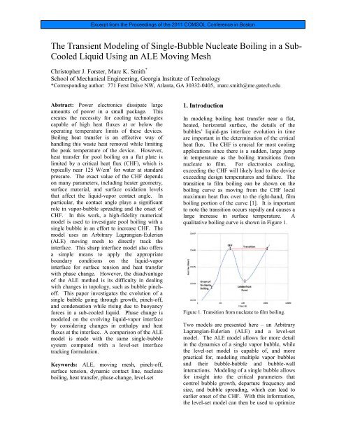
In modeling boiling heat transfer near a flat,
heated, horizontal surface, the details of the
bubbles’ liquid-gas interface evolution in time
are important in the determination of the critical
heat flux. The CHF is crucial for most cooling
applications since there is a sudden, large jump
in temperature as the boiling transitions from
nucleate to film. For electronics cooling,
exceeding the CHF will likely lead to the device
exceeding design temperatures and failure. The
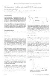
transition to film boiling can be shown on the
boiling curve as moving from the CHF local
maximum heat flux over to the right-hand, film
boiling portion of the curve [1]. It is important
to note the transition occurs rapidly and causes a
large increase in surface temperature. A
qualitative boiling curve is shown in Figure 1.
Figure 1. Transition from nucleate to film boiling.
Two models are presented here – an Arbitrary
Lagrangian-Eulerian (ALE) and a level-set
model. The ALE model allows for more detail
in the dynamics of a single vapor bubble, while
the level-set model is capable of, and more
practical for, modeling multiple vapor bubbles
and their bubble-bubble and bubble-wall
interactions. Modeling of a single bubble allows
for insight into the critical parameters that
control bubble growth, departure frequency and
size, and bubble spreading, which can lead to
earlier onset of the CHF. With this information,
the level-set model can then be used to optimize

heater configurations in more practical and
complicated cooling applications.
2. Use of COMSOL Multiphysics
2.1 Initial Model Geometry, Initial
Conditions, and Boundary Conditions
The bubble begins as a spherical-cap, attached
bubble at the bottom of the tank. The initial
configuration is shown in Figure 2. The gravity
force and heat flux are ramped in over relatively
short time scales, 0.05s and 0.1s, respectively.
This allows the solver to start more easily, and it
allows condensation to be more directly
observable before the heat flux input to the
bottom of the tank has been fully ramped in.
The temperature profile is initially linearly
varied from saturation temperature at the hot
surface to a sub-cooled temperature at the upper
boundary. The amount of sub-cooling can be
adjusted, but for this model it is set at 5K, which
is reasonable for boiling experiments. The initial
velocity field is zero, and the initial pressure
field is uniform over each subdomain, with the
bubble pressure increased by the Laplace
pressure jump. This pressure field is appropriate
for zero initial gravity, before gravity is ramped
in, and the equilibrium, spherical-cap bubble
shape. The model is axisymmetric.
Figure 2. Initial model configuration.
The hydrodynamic boundary conditions will be
listed first. The hot plate is modeled as a slip
boundary with a fixed contact angle, but each
domain can be set to slip or no-slip
independently. Future models may incorporate a
contact line mobility model to more accurately
capture the contact line dynamics, but for now
the two extremes of slip and no-slip are easily
modeled. The upper tank boundary is set to zero
gage pressure. The right-hand tank wall is set to
a slip boundary condition. The vapor-liquid
interface enforces a no-slip condition for the
tangential velocity component. The normal
velocity component accounts for the divergence
due to vaporization occurring at the interface.
The Young-Laplace normal stress jump is
modeled. The vapor recoil pressure can be
included, but it was chosen to be neglected in
this model. The inclusion of vapor recoil
pressure makes the model more unstable, and for
lower heat inputs, the vapor recoil pressure is
negligible. Vapor recoil pressures were observed
to be on the order of 1 Pa while pressure from
surface tension is approximately 50 Pa. The
vapor recoil effect may be more significant at
higher heat inputs.
In each thermal domain, the interface is required
to remain at the saturation temperature, which is
prescribed to be 373.15K to represent boiling at
standard pressure. The saturation temperature
can be a function of pressure, but the slight
variations in saturation temperature due to
pressure variations are neglected here. The
energy balance at the interface is maintained by
the rate of vaporization or condensation. The
heat fluxes are calculated on each side of the
interface and the difference determines the rate
of vaporization or condensation. The hot plate
has a heat flux input prescribed to be 0.2 W/cm 2
under the vapor bubble and 20 W/cm 2
everywhere else. This choice is somewhat
arbitrary, and the reason behind choosing a nonuniform
heat flux is discussed in the results
section. The model can be modified to include
another domain for the heat transfer model of the
solid heater plate to determine the distribution of
heat between the bubble and the surrounding
liquid. This paper is focused on presenting the
interface conditions and modeling of the phasechange,
so the additional domain for the heater
plate is omitted for clarity. The right-hand side
of the tank is modeled as thermally-insulated.
The upper tank boundary is held at the saturation
temperature minus the amount of sub-cooling,
which is 368.15K for this model.

2.2 Pinch-off Transition
Leading up to pinch-off the ALE model is run
with remeshing periodically to maintain mesh
quality. The pinch-off point is chosen near the
minimum neck radius for this simulation. A
reasonable gap height is chosen between the
attached and pinched bubble to prevent creating
excessively small elements in the pinched region.
The final geometry of the attached bubble
simulation is exported to Matlab as an array of
points with the pinch-off points inserted. The
boundary points are spline-fit with constraints on
end-point tangency. The geometry is imported
back into Comsol and boundary conditions are
transferred from the previous geometry. The
number of fluid domains increases from two to
three domains. Since a finite amount of time
occurs during pinch-off, which is not modeled
here, post-pinch-off velocity, pressure, and
temperature fields were estimated in order to
continue the simulation. These estimated initial
conditions after pinch-off are an attempt to
demonstrate that it is possible to continue the
new model where the previous model ended.
The pinch-off criteria will be improved in future
work. The idea is that when the bubble neck is
small enough, the pinch-off process will be
computed analytically using a separate
asymptotic model. This will reduce numerical
computational requirements due to meshing
regions of relatively small length scales
compared to the rest of the model. After pinchoff,
the shape of the gas bubbles and the
associated velocity and pressure fields near the
pinch-off point will be used to reinitialize the
numerical model and continue the simulation.
2.3 Governing Equations for the ALE Model
The incompressible Navier-Stokes and
advection-diffusion equations are solved over
each domain. Including the ALE moving mesh,
there are five domains or application modes
modeled in Comsol that are coupled with
boundary conditions. The Boussinesq
approximation is used to allow natural
convection with the incompressible fluid model.
The ALE method only requires boundary
conditions to be specified to link the liquid and
vapor domains and account for vaporization.
This is different than having to formulate volume
forces and sources as is required in a fixed-mesh
method.
The first step in formulating these boundary
conditions is to prescribe the mesh motion so
that it follows the interface evolution. The mesh
interface velocity is not the same as either the
local vapor or liquid velocities since there is an
influx/outflux of each relative to the interface,
depending on if there is local vaporization or
condensation. The mesh is allowed to slide
tangentially along the interface to allow for
improved mesh quality as deformation takes
place, so only a normal component needs to be
specified. The normal components are denoted
with a subscript ‘n’. The normal vector
convention is that the outward facing normal
vector is positive, and each domain has its own
outward normal. A diagram of the domain and
normal vectors are shown in Figure 3. The
normal velocity of the mesh is given by
̂ (1)
Figure 3. Liquid and Vapor domains with labeled
boundary conditions and heat flux input at hot plate.
where is the relative normal liquid velocity
to the interface, and it is calculated by taking the
difference of heat flux on each side of the
interface and using liquid and vapor enthalpies
and densities in the calculation. The sign
convention used assumes vaporization has a
positive liquid velocity relative to the interface
(i.e., liquid influx is positive). This calculation
will be discussed in more detail later, after the
thermal boundary conditions.

The next step is to couple the vapor and liquid
domain velocities at the interface. The tangential
components are equal, assuming a no-slip
condition. The normal components differ by the
sum of the magnitudes of the vapor and liquid
velocities relative to the interface (i.e., the
relative velocities are defined with the observer
attached to the moving interface). These
constraints, in terms of normal components, are
shown in Eqn. 2 and 3.
( ̂) ( ̂) (2)
( ̂ ̂ ) (3)
The interface temperatures, in both the liquid and
vapor domains, are set to the local saturation
temperature as Dirichlet boundary conditions.
(4)
With radiation neglected, the amount of heat
going into vaporization is the sum of the
conduction heat transfer into the inner and outer
sides of the interface.
̂ ̂ (5)
The relative or flux velocities can now be
calculated using additional property data that can
be temperature and pressure dependent. The
property data can be represented with a curve-fit
or table interpolation.
( )
( )
(6)
(7)
Vapor recoil may be included by adding the
following terms to the stress boundary condition
on the vapor domain along the interface. The
boundary stress terms are separated into
projected components to allow for incorporation
into the weak form of the Navier-Stokes
equations in Comsol Multiphysics. The
velocities in Eqn. 8 are relative to the interface.
[
]
( ̂ ) ( ̂ ) (8)
The normal-stress boundary condition on the
liquid-gas interface is
( ) ̂ ̂ , (9)
where are the stress tensors for the gas and
the liquid, defined as
[ ( ( ) )]
(10)
̂ is the outward unit normal to the gas-liquid
interface, is the surface tension of the interface,
and is the curvature of the interface defined as
̂, (11)
where is the surface divergence operator. The
Navier-Stokes equations on the sub-domains
remain unchanged since the surface tension is
implemented as a boundary condition.
Multiplying both sides of Eqn. 9 by a test
function and integrating results in,
∫ ( ̃ ̂)
∫ ( ̃ ̂)
∫ ( ̃ ̂)
(12)
Applying the surface divergence theorem [2] to
the last surface integral on the right-hand side
and substituting back in yields,
∫ ( ̃ ̂)
∫ ( ̃ ̂)
∫ ( ̃)
∫ ( ̃ ̂)
(13)
where ̂ is a unit binormal vector at the contact
line, and ̃ is a test function.
This last equation can be applied as boundary
and point weak expressions in Comsol. This
applies to 2D, 2D axisymmetric, and 3D models,
although some minor modifications need to be
made to express this in polar coordinates.
2.4 Governing Equations for the Level-set
Model
The finite element level-set model incorporates
phase change in a method similar to Son and
Dhir [3,4], except that a ghost fluid method
cannot be implemented in Comsol Multiphysics
for calculating heat fluxes on the interface. To

account for phase change, terms are added to the
continuity and energy equations only on the
interface using a delta function. Vapor recoil is
accounted for, similarly, by adding a term to the
momentum equation, again only on the interface
using a delta function. The temperature recovery
method described in [5] is used to maintain the
saturation temperature on the interface, where
the level-set variable is 0.5. Comsol
Multiphysics uses a level-set variable that varies
between 0 and 1, as opposed to -1 to 1. The first
use, to the best knowledge of the author, of the
temperature recovery method appears in [6].
The temperature recovery method works by
proportionally increasing the mass vaporization
(condensation) rate as the local interface
temperature deviates from the saturation
temperature. This is solved at each time step
inside the Comsol solver along with the velocity,
temperature, and level-set fields. In effect, the
temperature recovery method determines the
amount of fluid vaporization (condensation)
required to maintain the interface temperature,
rather than calculating the mass vaporization
(condensation) rate directly from the temperature
gradients on each side of the interface, since
these gradients are not available and not
accurately computed without using a ghost fluid
method. The mass vaporization (condensation)
rate calculated from heat fluxes at the interface
should, in theory, dictate enough vaporization
(condensation) to keep the interface at saturation
temperature. With this in mind, determining the
mass vaporization (condensation) rate to some
value that is enough to maintain the interface
temperature at saturation should lead to the same
result. The temperature recovery method has
been verified to maintain interface temperatures
within approximately 0.3 °C. The finite element
model utilizes quadratic triangular (tetrahedral
for 3D) Lagrange elements for the fluid, thermal,
and level-set equations. The present model does
not account for thin film (micro-scale) boiling,
but a lubrication model can be added in Comsol
Multiphysics and coupled to the current model.
Aside from the temperature recovery method for
determining the mass vaporization
(condensation) rate, the formulation is very
similar to Son and Dhir’s method [3], which is as
follows.
First, the mass vaporization (condensation) rate
is determined from the interface temperature
profile, shown in Eqn. 14. Note that ̇ is per
unit interface surface area. The proportionality
constant ‘C’ can be adjusted if the vaporization
(condensation) rate is insufficient to maintain
saturation temperature on the interface. Setting
this constant too large will lead to numerical
instabilities.
̇ (
) (14)
Also, the mass vaporization (condensation) rate
can be formulated as an interfacial normal flux,
which is used for the continuity source term on
the interface,
̇ ( ) ̂ (15)
where U is the interface velocity and the
subscript ‘f’ indicates the fluid, which could be
liquid or vapor. The next step is to evaluate Eqn.
15 for both the liquid and vapor, and then
rearrange for the liquid and vapor velocities.
Equations 16 and 17 represent the normal
components only – vector notation is omitted for
clarity.
̇ (16)
̇ (17)
Taking the difference in the liquid and vapor
velocities at the interface provides the
divergence created by the phase-change and
corresponding change in density. The fluid is
treated as incompressible everywhere in the
fluid, except on the interface region, and the
continuity source term is Eqn. 18 multiplied by
an interface delta function that only allows the
source term to be non-zero on the interface.
(
) ̇ ̂ (18)
The continuity equation with the additional
source term is shown in Eqn. 19 and 20, where
is the interface delta function.
( ) (19)
(
) ̇ ̂ (20)
The tangential stress on the vapor and liquid
sides of the interface are equal while there is a

jump condition in the normal stress. The normal
stress changes across the interface because of the
effects of surface tension and vapor recoil. Eqn.
21 prescribes that the tangential stress on each
side of the interface is equal. Eqn. 22 is the
normal stress jump condition.
̂ [ ( ) ( ) ] ̂
̂ [ ( )
( ) ] ̂
(
) ̇
(21)
(22)
The forces from surface tension and vapor recoil
are added to only the interface region as volume
force terms using the interface delta function.
The next step is to account for the latent heat of
vaporization in the energy equation. This is
done by adding a term, multiplied by the
interface delta function, to account for the energy
liberated (absorbed) by condensation
(vaporization). The modified energy equation is
shown in Eqn. 23, where is the latent heat of
vaporization.
(
) ( ) ̇
(23)
The level-set function is updated since it only
accounts for advection of the interface by default
– it does not account for interface movement as
vapor phase is generated. The modified level-set
function is shown in Eqn. 24.
where,
̇
(24)
̂ (25)
This completes the necessary modifications to
the finite-element level-set model, and it now
accounts for vaporization and condensation.
3. Results and Discussion
The single-bubble models use an initial bubble
radius of 3 mm. The surface tension coefficient
is 0.07 N/m for all models. Pressure and gravity
are 1atm and 9.81 m/s 2 , respectively.
3.1 ALE Results
The heat flux input over the heater surface
exposed to liquid is 20 W/cm 2 and the region of
the heater surface underneath the vapor bubble is
0.2 W/cm 2 . The exterior contact angle is 55
degrees. The heat flux is ramped in over 0.1 s.
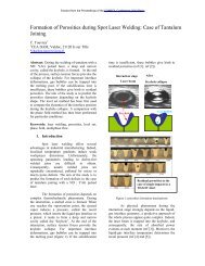
The model is axisymmetric. Figure 4 shows the
temperature distribution with velocity arrows
over-plotted and the interface marked with a
white line at selected time steps.
Figure 4. ALE simulation results for a contact angle of
55 degrees.
The vapor in the bubble reaches relatively high
temperatures even at low heat fluxes. The model
was run with 0.2 W/cm 2 input under the vapor
bubble to reduce the peak temperatures in the
vapor domain, which were observed to be in
excess of 1000 K at higher heat fluxes. The
reduced heat flux under the vapor bubble limits
peak vapor temperatures to approximately
450 K. The next step is to include another heat
transfer domain to incorporate the solid heater
plate. This will allow for a physical
determination of the appropriate heat distribution
under the vapor bubble and the rest of the heater
surface exposed to liquid. The liquid and vapor
have significantly different thermal
conductivities, so the heat flux is not expected to
be uniform over the entire heater. However, the

heater plate will physically smooth out
temperature gradients along the surface of the
heater and between the vapor and liquid. This is
expected because of the higher thermal
conductivity in the solid heater plate compared to
water in both liquid and vapor states.
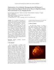
The ALE method can also model a pinned
contact line with phase-change. Figure 5 shows
the results from the pinned contact-line model.
Figure 5. ALE results for a pinned contact line.
The non-isothermal ALE model requires more
remeshing to reach pinch-off than the previous
isothermal model [7]. This appears to be
primarily due to the addition of vaporization and
condensation on the interface. The pinch-off
process was not successful due to the solver
being unable to restart with the current
approximated solution on the new geometry after
pinch-off. This is likely to be because the
approximated solution created did not satisfy the
model constraints and boundary conditions
within solver tolerances. The intermediate
model proposed would provide a more accurate
solution to resume the model after pinch-off. It
is expected that this would be successful in
continuing the model after pinch-off.
3.2 Level-Set Results
The heat flux input over the entire surface of the
hot plate is 15 W/cm 2 . The exterior contact
angle is 55 degrees, and the hot surface enforces
a slip length condition. The model was
performed in 3D and utilized symmetry
conditions to minimize the computational
domain. A 1/8 th vertical wedge was modeled.
This provides similar results to the axisymmetric
case in the ALE model. The mesh resolution is
relatively coarse in the level-set model to reduce
computational expense. This is likely to make
the solution mesh-dependent, especially near the
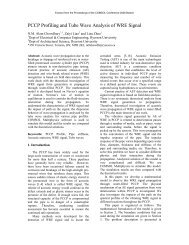
contact line. The results in Figure 6 show the
iso-surfaces of the level-set function values of
0.5. The heat flux input is started immediately,
without ramping in. The liquid is sub-cooled by
5K at the upper tank boundary, and the initial
temperature condition is a linear profile from
saturation temperature at the hot surface to the
sub-cooled temperature at the upper tank
boundary.
Figure 6. 3D, 1/8-symmetry model of a single vapor
bubble.
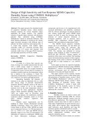
The level-set model can be extended to multiple
vapor bubbles. The next results shown in Figure
7 were performed in 2D to minimize
computational expense. While the 2D model
neglects the second curvature used for
calculating pressure due to surface tension, it
does provide qualitative results for the behavior
of the interactions between bubble interactions
and departure frequency.
Figure 7. 2D simulation of three nucleation sites.

The level-set reinitialization parameter needs to
be chosen carefully since the default value in
Comsol Multiphysics 4.2 tends to introduce a
significant amount of interface movement due to
accumulation of error in the reinitialization
procedure that occurs at each time step. The
value of the reinitialization parameter is specific
to each problem. It has been found that values
on the order of 0.01 or less provide the best
results. The amount of error accumulation was
determined by running level-set models with a
geometry undergoing rigid body rotation and/or
translation. The rigid body movement was
achieved by prescribing a velocity field that
forced rigid body rotation or a uniform velocity
field to provide rigid body translation. With the
rigid body motion prescribed, the only source of
deformation from the original geometry is from
error accumulation due to the reinitialization of
the level-set function at each time step.
4. Conclusions
The ALE model needs more refinement to allow
for a successful pinch-off procedure. It is likely
that the approximated solution, for restarting the
model with the post-pinch-off geometry, does
not satisfy model constraints within the solver
tolerances. The approximate solution attempted
here was made by taking the solution at the last
time step before pinch-off and performing local
modifications to approximate the solution a
small finite time after the initiation of pinch-off.
This worked in the previous model [7], but this
model has a key difference of having
discontinuous velocity fields. There is a jump in
velocity at the interface due to phase change, so
mapping the solution to the new geometry is
more difficult. It is expected that including an
intermediate pinch-off model will provide a
more accurate solution and alleviate the
inconsistent initial solution problem when
resuming the model.
The ALE model allows for more control over the
contact line dynamics. A contact line mobility
and hysteresis model can be included to
determine the transition from pinned to dynamic
contact line movement. The level-set model
allows for boundary conditions to be modified at
the weak level in Comsol Multiphysics, but since
the interface is smeared over a distance on the
order of one mesh element length, the control
over the contact line is less precise.
The ALE method allows for a more physical
approach for determining the rate of vaporization
(condensation) at the liquid-vapor interface and
for more detail of the contact line dynamics.
However, when it comes to modeling more
complicated heater surfaces or interactions of
multiple vapor bubbles, the level-set model is
more practical. The level-set model
compliments the ALE model, and by using both,
modeling of the finer detail of the dynamics of a
single bubble and interactions of many vapor
bubbles and nucleation sites on more
complicated geometry is possible.
5. References
1. Incropera, F. P., & DeWitt, D. P. (2002).
Introduction to heat transfer. (4th ed., pp. 558-563).
New York: John Wiley & Sons.
2. C.E. Weatherburn, Differential Geometry of Three
Dimensions, 238-242, University Press, Cambridge
(1955).
3. Son, G. & Dhir, V. K. (2007). A level set method
for analysis of film boiling on an immersed solid
surface. Numerical Heat Transfer: Part B, (52), 153-
177.
4. Son, G. & Dhir, V. K. (2008). Numerical simulation
of nucleate boiling on a horizontal surface at high heat
fluxes. International Journal of Heat and Mass
Transfer, (51), 2566-2582.
5. Tsujimoto, K. , Kambayashi, Y. , Shakouchi, T. &
Ando, T. (2009). Numerical simulation of gas-liquid
two-phase flow with phase change using cahn-hilliard
equation. Turbulence, Heat and Mass Transfer, 6, 1-
12.
6. T. Kunugi, N Saito, Y. Fujita and A. Serizawa.
Direct Numerical Simulation of Pool and
Forced Convective Flow Boiling Phenomena, Heat
Transfer 2002, 3:497-502, 2002
7. Christopher J. Forster and Marc K. Smith, The
Transient Modeling of Bubble Pinch-Off Using an
ALE Moving Mesh, Comsol (2010)