Download Paper - COMSOL.com

Formation of Porosities during Spot Laser Welding: Case of Tantalum
Joining
C. Touvrey 1
1 CEA DAM, Valduc, 21120 Is sur Tille
*charline.touvrey@cea.fr
Abstract: During the welding of tantalum with a
ND: YAG pulsed laser, a deep and narrow
cavity, called the keyhole, is formed. At the end
of the process, surface tension forces provoke the
collapse of the keyhole. For important interface
deformations, gas bubbles can be trapped into
the melting pool. If the solidification time is
insufficient, these bubbles give birth to residual
porosities. The aim of the study is to predict the
porosities diameters depending on the keyhole
shape. The level set method has been first used
to compute the dynamics of the interface position
during the keyhole collapse. A comparison with
the phase field method has then been performed
for particular conditions.
Keywords: laser welding, porosities, level set,
phase field, multiphase flow.
1. Introduction
Excerpt from the Proceedings of the COMSOL Conference 2010 Paris
Spot laser welding offers several
advantages in industrial manufacturing. Indeed,
localized temperature gradients induce weak
workpieces distortions. Unfortunately, the
operating parameters leading to defect-free
welded joins are difficult to obtain.
Consequently, unsafe welded joins are
repeatedly encountered, polluted by micro or
macro pores defects. The aim of the study is to
predict the formation of such defects in the case
of tantalum joining with a ND : YAG pulsed
laser.
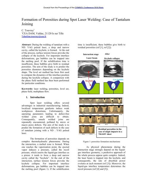
The formation of porosities depends on
complex thermohydraulic phenomena. During
the interaction, a melted zone is formed. When
one reaches the vaporization point, the ejected
vapor induces a pressure, called the recoil
pressure, which inserts the liquid-gas interface as
a piston: it tends to form a deep and narrow
cavity called the “keyhole”. At the end of the
interaction, surface tension forces provoke the
keyhole collapse. For important interface
deformations, gas bubbles can be trapped into
the melting pool (figure 1). If the solidification
time is insufficient, these bubbles give birth to
residual porosities (ref [1], ref [2]).
Interaction stage
Laser beam
Keyhole
After
interaction:
Keyhole collapse
Gas bubble
Residual porosities in the
case of single impacts in a
Ti6Al4V sheet
Figure 1: porosities formation mechanisms
As physical phenomena during the
interaction stage strongly depend on the liquidgas
interface geometry, a predictive approach of
the whole process appear quite complex. Indeed,
the laser beam is trapped into the keyhole, and
consequently, the rate of absorbed power
evolutes at each moment (ref [3]). Moreover, the
liquid-gas interface temperature determines the
recoil pressure (ref [4] and [5]).

That’s why, for our problem, we have
focused our attention on the cooling stage. The
mechanisms of keyhole collapse have been
apprehended thanks to a hydraulic model.
Following a parametric analysis, we are trying to
find a depth limit, from which gas bubble are
always trapped. The following model have been
originally developed by K. Girard and J. Nadal
(ref [6]) in the software FLUENT. Unfortunately
many numerical problems have been
encountered by the authors, especially induced
by interface instabilities.
2. Physical model
2.1 Shape of the keyhole at the end of the
interaction
As we only model the cooling stage,
the geometry ok the keyhole at the end of the
interaction must be determined.
First of all, the position of the fusion
isotherm is deduced from a metallurgical
analysis, as shown on figure 2. Moreover, the
keyhole’s ray, and the volume of metal
accumulated at the surface, is measured
according to visualizations of the melting pool
with a high speed camera (figure 3). At last, K.
Girad (ref [6]) proposes a good approximation of
the liquid film dimension at the bottom of the
keyhole (about 40 µm in our case).
0,38 mm
Figure 2: metallurgical analysis
Figure 3: visualization of the keyhole
In the model, we admit that the shape of
the keyhole is ½ elliptic and that the metal
accumulated at the surface tends to form a tore.
By writing that the volume of the ½ tore is equal
to the ½ ellipse’ one, we are able to deduce all
the problem dimensions.
2.2 Materials properties
In the case of liquid tantalum, the density ρ is
equal to 15630 kg/m 3 and the dynamic viscosity
μ is equal to 8.032e -3 Pa·s. The surface tension
coefficient is taken equal to 2.168 N.m -1 .
1.2 Hypothesis
The surface tension coefficient is supposed
constant during the collapse stage. Characteristic
dimensionless numbers calculation shows that:
- the flow is laminar;
- capillary effects are important
-
compared to viscous ones:
V
3
Ca 2.
10
ts
gravity effect can be neglected:
g.
L²
Bo 8.
10
ts
3. Governing Equations
The level set method has been first used
to determine the evolution of the interface
position. A comparison with the phase field
method has then been performed for particular
conditions.
The Level Set application mode is
largely described in ref [7]. The method enables
to find the fluid interface by tracing the isolevel
of the level set function, Φ. The isocontour Φ
=0.5 determines the position of the interface. The
equation governing the transport of Φ is:
where u (m/s) is the fluid velocity, and γ
(m/s) and ε (m) are numerical stabilization
parameters. The ε parameter determines the
thickness of the layer around the interface where
4

Φ goes from zero to one. ε is generally taken
equal to hc/2, where hc is the characteristic mesh
size in the region passed by the interface..
Generally, a suitable value for γ is the maximum
velocity magnitude occurring in the model.
In the Phase Field application mode
(largely described in ref [7]), the two-phase flow
dynamics is described by the Cahn-Hilliard
equation. The method consists in tracking a
diffuse interface separating the immiscible
phases (region where the dimensionless phase
field variable Φ goes from −1 to 1). The Cahn-
Hilliard equation is solved in two times:
where u is the fluid velocity (m/s), γ is
the mobility (m3·s/kg), λ is the mixing energy
density (N), and ε (m) is the interface thickness
parameter. The mixing energy density and the
interface thickness are related to the surface
tension coefficient through the relation (réf 8):
ε is usually set to half the characteristic
mesh size in the region passed by the interface.
The mobility parameter γ determines the time
scale of the Cahn-Hilliard diffusion and is
generally taken equal to ε 2 .
In both the two methods, the transport
of mass and momentum is governed by the
incompressible Navier-Stokes equations,
including surface tension:
In the above equations, ρ (kg/m3) denotes the
density, u the velocity (m/s), t the time (s), p the
pressure (Pa), and η denotes the dynamic
viscosity (Pa·s). The momentum equations
contain gravity, ρg, and surface tension force
components, denoted by Fst. But, in our case,
gravity is neglected.
The surface tension force is
implemented differently in the Level Set and
Phase Field application modes (ref [7]). The
Level Set application mode computes the surface
tension as:
where ζ is the surface tension
coefficient, I is the identity matrix, n is the
interface unit normal, and δ is a Dirac function,
nonzero only at the fluid interface. The interface
normal is calculated from:
The level set parameter Φ is also used to
approximate the delta function by a smooth
function defined by:
In the Phase Field application mode, the
diffuse interface representation implies that it is
possible to compute the surface tension by:
where Φ is the phase field parameter,
and G is the chemical potential (J/m3):
4. Numerical Model
4.1. Initial state
The initial state is deduced from
observations and hypothesis made in
paragraph 2.1. The initial interface
geometry is described in figure 4.

0,34 mm
0,04 mm
Figure 4: initial state
4.1. Boundary settings:
The boundary conditions are presented on figure
5.
Axial
symmetry
0,43 mm
Air
0,32 mm
Liquid
tantalum
Figure 5: boundary settings
0,14 mm
Open boundary
Wetted wall
For the level set method, the wetting phenomena
are determined by the contact angle and the slip
length. The velocity component normal to the
wall is set to zero:
One adds a frictional boundary force:
β is called the slip length. The angle between the
wall and the fluid interface, called the contact
angle θ, is supposed constant equal to pi/2. By
default, the slip length is equal to the mesh
element size, h. We will see thereafter the
consequences of this dependence.
For the comparison between the level set and the
phase field method, the condition “wetted wall”
has been replaced by a “slip wall” condition.
4.2. Meshing
The mesh must be homogenous along the liquid
– gas interface in order to initialize correctly the
problem. In order to analyse the model spatial
convergence, the mesh size has been
progressively reduced. When the mesh is
consequently refined, the air domain size must
be extended to obtain a converged solution.
4.4 Choice of level set parameters
In the present model, the mesh size is inferior to
1e-5. Consequently, the value of ε has been fixed
to 5e -6 and γ is equal to 1. Indeed, thanks to
experimental measure, the velocity of the fluid
doesn’t exceed 1 m.s -1 .
4.3. Transient initialization:
Before starting the fluid flow calculation, the
level set function must be initialized. The
initialization time is fixed to 5ε/.
5. Results and discussion
Firstly, the numerical behaviour of the model has
been tested for a high dynamic viscosity (8 Pa.s).
This allows a better model convergence. Some
results are presented on the figure 6.
The filling of the keyhole can be divided into
two stages: a “detachment stage”, illustrated on
figure 6.c, and a “filling stage”, illustrated on
figure 6.d.

Figure 6: numerical results: keyhole
collapse
a
b
c
d
The results are stable while reducing the
mesh size from 1.3.10 -5 to 3.1.10 -6 . Nevertheless,
the detachment stage length increases while
refining the mesh (board 1). It can be explained
by the dependence between the mesh size and
the slip length. Consequently, the slip length will
have to be determined by comparison with
experimental data (figure 7).
Minimum detachment Filling stage
mesh size stage duration duration
1.3e-5 5 10
6.4e-6 6 11
3.1e-6 7 13
Board 1: spatial convergence
Thanks to a parametric analysis, it is
confirmed that the gravity has no influence. The
flow is laminar, with a maximum velocity of 0.5
m.s -1 . It asserts the good choice of = 1.
The complete filling time, about 20 ms, is
longer than expected. Indeed, a high speed
camera film shows that the keyhole collapse
doesn’t exceed 1 ms (figure 7). This can be
explained by the non physical value of the fluid
viscosity.
Figure 7: experimental results: keyhole collapse
A computation has then been performed with the
phase field method. Neglecting the wetting
phenomena, it confirms the interface shape

obtained by the level set application mode. The
sliding condition between the solid and the fluid
induces a collapse time of 8 ms in the two cases.
Considering the real viscosity of the fluid
(8.032e -3 Pa.s -1 ) makes the model convergence
difficult to obtain. Indeed the liquid film
undergoes a thinning (figure 8) and the mesh size
must be consequently reduced to allow the
convergence. The results are stable while
refining the mesh. Nevertheless, the interface
shape does not seem physically correct, and this
part of the study will have to be reconsidered.
Figure 8: interface shape with the real viscosity
6. Conclusions
In order to predict the risk of porosities
formation during tantalum welding, a model has
been developed to simulate the keyhole collapse.
Two Eulerian methods have been used and
compared: the Level set and Phase Field
methods.
If the interface shape seems to be physically
correct for a high fluid viscosity, the liquid film
undergoes a thinning when considering the real
tantalum viscosity (8.032e-3 Pa.s -1 ). This
phenomenon has to be studied, especially by
comparing different numerical methods.
In order to evaluate the diameter of the
pores that may affect our welded joints, we are
currently working on a second model to simulate
the bubbles up rise simultaneously with the
solidification front progress (thermo-hydraulic
approach).
7. References
1. Girard, K., Jouvard, J.M., Boquillon, J., Bouilly, P.,
and Naudy, P., 2000, SPIE Conf. (Bellingham,
SPIE), 3888, pp. 418-28.
2. Kaplan, A., Mizutani, M., Katayama, S., and
Matsunawa, A., 2002, Unbounded keyhole
collapse and bubble formation during pulsed laser
interaction with liquid zinc, J. Phys. D: Appl.
Phys., 35, pp. 1218-1228.
3. Medale, xhaard, guignard “A Thermo-Hydraulic
study of a thin metal plate submitted to a single laser
pulse”, Proceedings of 4th ICCHMT, May 17–20,
2005, Paris-Cachan, FRANCE
[4] W. Semak, W.D. Bragg, B. Damkroger, S.
Kempkas, Temporal evolution of the temperature
field in the beam interaction zone during lasermaterial
processing, J. Phys. D: Appl. Phys. 32
(1999) 1819-1825.
[5] P. Solana, P. Kapadia, J.M. Dowden, P.J.
Marsden, An analytical model for laser drilling of
metals with absorption within the vapour, J. Phys.
D: Appl. Phys. 32 (1999) 942-952.
[6] Karen Girard, “étude de la formation des porosités
dans les soudures de tantale par laser ND:YAG
impulsionel”, thèse, 1999
[7] Bubble rising, COMSOL documentation
[8] P. Yue, J. Feng, C. Liu, and J. Shen, “A Diffuse-
Interface Method for Simulating Two-Phase Flows of
Complex Fluids,” J. Fluid Mech., vol. 515, pp. 293–
317, 2004.
[9] C. Touvrey, “étude thermohydraulique du soudage
impulsionnel de l’alliage TA6V ” thèse, 2006
8. Acknowledgements
Thanks to JM. Petit, from COMSOL company,
who has developed the original model of
keyhole’s collapse in the case of high fluid
viscosity.
Thanks to R Fabbro and K Hirano, from ARTS,
who have realized the visualization of the
melting pool with a high speed camera.