High Vacuum Gas Pumping and Boundary Coupling - COMSOL.com

High Vacuum Gas Pumping and Boundary
Coupling
Marco Cavenago
INFN/LNL, Laboratori Nazionali di Legnaro
viale dell’Universita’ n. 2, I-35020 Legnaro (PD) Italy, cavenago@lnl.infn.it
Abstract:
The gas flow in the low pressure limit,
named molecular flow regime, is a case of
transport with zero viscosity. As an alternative
to Monte Carlo methods typically used
to estimate pipe conductance, an integral
boundary equation (IBE) is here discussed,
and solved, at least for simple 2D geometries
(a circular junction and a simple pipe
obstruction). An ad hoc algorithm to find
obstacles on the view lines was developed
for the latter case. The particular cares requested
at the corners and in the interpolation
from boundary to inner domain are
shown. Relation between flow and pressures
at ports is discussed, with the usual cosine
law for the distribution of the velocities at
input. For the circular junction, a typical
PDE (partial differential equation) is here
shown to have the same solution of the IBE,
which allows for a comparison of the numerical
precision of both approaches, showing a
good agreement.
Keywords: molecular flow, gas pumping,
integral equation
1 Introduction
Excerpt from the Proceedings of the COMSOL Conference 2008 Hannover
Many scientific instruments are based on
high vacuum equipment[1], with a gas pressure
maintained in the order of 1 Pa or below
by suitable pumps; ionization is possible,
so that a plasma may be also formed. The
gas pressure p in the vacuum chamber is of
fundamental importance in all applications
and depends on the size of the pipes connecting
the vacuum chamber to the pumps.
Two major regimes exists[2], depending on
the Knudsen number Kn (ratio between geometry
size D and mean free path λ ): viscous
(Kn > 80), which includes turbulent
and laminar flow, and molecular (Kn < 3).
Pressure p in the molecular regime is usu-
ally estimated by practical rules based on a
lumped model of pipe conductances, which
sometimes is a poor approximation for realistic
shapes.
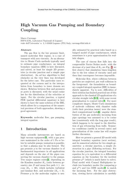
The case of viscous flow falls into the
compressible Navier Stokes mode: with the
decrease of p (and thus of Kn see Fig. 1) we
first observe that simulation times lengthen
due to the low values of viscosity used and
then that convergence becomes impossible.
Molecular flow, where collisions between
particles are neglected, put wall collisions in
the foreground: the formulation as boundary
coupled integral equation (IBE) is immediately
apparent. Up to now, difficulties of
their solution has limited practical use of this
approach to the classical 1D applications of a
circular straight tube[3, 4], with some recent
generalization to conical tubes[5]. For more
complicate shapes, Monte Carlo simulations
of molecule collisions with chamber walls
(with their precision issues) were the standard
computational tools[6]: angular distribution
of the gas molecules incoming from
pipe openings was assumed to a be cosine
law (consistently with the long pipe result),
which happens to be equal to the distribution
of gas rebouncing from walls. Symmetry
conditions (useful in several cases) and
generalization of the cosine law will require
further discussion.
Here we present a general 2D model with
integral boundary equation (next section),
and its numerical solution for two simple geometries:
a circular junction, a simple obstruction
in a pipe (following sections). For
the circular junction, the integral boundary
equation for p is equivalent to a differential
equation on the boundary for the incident
pressure p in (which is much faster to solve).
Final model with Comsol Multiphysics include
two boundary modes (for comparing p
and p in ) and two ODE modes[7] to match
the incoming flow. For the pipe obstruction,
viewing factor calculation is carefully

optimized with some scripting. Remarks on
the generalization to 3D are discussed in the
conclusion.
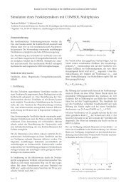
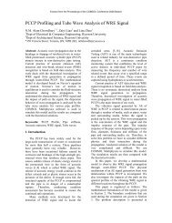
Figure 1: Sketch of viscosity (arbitrary units),
Reynolds number Re and Knudsen number Kn
vs pressure p
2 Molecular flow
The well known ideal gas law p = nkBT relates
the isotropic pressure of a gas to the
number density of molecules n and to the
temperature T , so that the mean free path
λ =
1
√ 2 nσ = kBT
√ 2pσ
(1)
is inversely proportional to the pressure;
here σ is the cross section of elastic collision
between molecules of mass m. The mass
density is ρ = n m = p m/kBT .
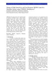
Figure 2: A generic planar geometry (if a
septum exists, this is excluded from the
simulation domain D). The point B is the
running integration point, while A is the
so-called destination or observation point
The average value of the modulus of the
velocity vav = (8kBT/πm) 1/2 is of course
different from the fluid velocity vf , which is
the average of velocities; roughly |vf | ≤ vav.
When λ ≪ D, where D is a typical diameter
of our pipe, the gas moves as a fluid,
according to the compressible Navier Stokes
equations (since mass density is proportional
to pressure), with a fluid velocity vf and a
viscosity
η = c3ρλvav = 2 −1/2 c3mvav/σ (2)
here c3 = 0.499 according to detailed transport
calculation [8]; note η is indipendent
from p in this regime.
When λ ≥ D/3, the pipe wall perturb
most of the gas motion, so that λ must be
replaced by c4D in equation (2), with the
estimate c4 ∼ = 0.5. Viscosity has to decrease
with pressure p → 0 . Figure 1 shows a
sketch of the dependence from p of η and
of the well known Reynolds number Re =
ρ vf D/η, which has the limit vf /c3c4vav ∼ = 1
for p → 0.
Let us restrict to a 2D planar geometry
as in Fig 2, where the simulation domain D
(closed, but necessarily simply connected or
convex) has solid walls and pipe openings
(Fig 3) as boundaries; for simplicity we will
not here discuss periodicity and/or symmetric
boundary conditions. At equilibrium, the
(numeric) flow density F in of particles incident
onto a wall
F in = nvav/4 = p in /(2πmkBT ) (3)
is related to the pressure p in incident on the
wall; in the following we will convert flows
to pressures by this proportion.
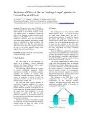
Figure 3: The example of a circular junction
At any point B on a solid wall, we assume
that the reemitted numeric flow F re
is equal to F in , and particle angular distibution
is f(ϑB) = 1
2 cos ϑB where ϑB is the
angle from the inward normal nB to the particle
direction (Fig 2). Let F vo the net volumetric
flow density (measured in [Pa m/s])
which enters from an opening; we assume
that the flow reeemitted F re is equal to F in

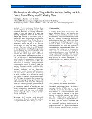
Figure 4: Elevation plot of simulation result for
p re and p in with p0 = f1 = 1 mPa
with the shorthand F ins = 4F vo /vav are the
basic relation of particle conservation. plus
the entering flow F vo /kBT . The equivalent
equations
F vo
kBT +F in and p re = F ins +p in (4)
Noting that any particle reemitted from
F re =
point B will incide at a point A, making an
angle ϑA with the inward normal nA, the
incident pressure is
p in A = L[p re
] = dsB
cos ϑB cos ϑA
p
2ϱ
re
BIAB
(5)
where the chord ϱ = xB − xA is the vector
from A to B and IAB is the viewing indicatrix:
equal to one if line segment AB is
not obstructed (by walls), otherwise equal
to zero. In particular, IAB = 0 if cos ϑB < 0
or if cos ϑA < 0, since these cases corrispond
to a chord passing into the walls.
Equations (4) and (5) are a formulation
of our problem with integral boundary equation
(IBE) only; references the pressure
Figure 5: Simulation results: contour and
surface plot of p i (note the r < 0.98r0 mask) ;
Here p3 = 2 mPa and p1 = 0.5 mPa, with the
result f1 = 0.825 mPa and p0 = 1.25 mPa
inside D is not necessary; anyway for postprocessing
we define the inner (or isotropic)
pressure at an inner point A as
p i A = M[p re
] = dsB
cos ϑB
2πϱ pre
B IAB (6)
this can be justified by balancing the in and
out flows on a circle of radius ɛ ∼ = h centered
at A, where h is the mesh element size; so
that eq. (6) holds strictly when distance wA
of A from walls is large enough:
wA ≡ min
B ϱ ≥ h(A) (7)
3 The circular junction
In the geometry of Fig 3, the simulation domain
D is the circle r ≤ r0; let (ψ, r) be the
polar coordinates and the output port P1 be
around ψ = 0, while gas may enter from the
other three ports. All points of the boundary
γ see each other, so IAB = 1; moreover
cos ϑB = sin(|ψA − ψB|/2) from simple geometry,
so that L simplifies to
L[p re ] = 1
π
4 dψB p
−π
re
B sin( 1
2 |ψA − ψB|) (8)
The expression (8) is directly implemented
as boundary integration variable
(’elle’) in Comsol Multiphysics, with destination
domain the boundary γ itself (here
ψA is the destination coordinate). The
boundary weak term looks like
bnd.expr=’test(p)*(elle+fins-p)’
Figure 6: Simulation results on the lower
boundary: p re as computed from the IBE eq
(8); p re from eq. (4), with p in computed from
the PDE equation (10).

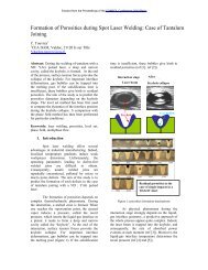
Figure 7: a) The simple obstruction, with a IAB = 0 ray in red; b) a detail of a corner
where the p re variable is typed ’p’. A first example
of solution for the case F ins = f1 = 1
mPa (millipascal) on port 3 (near ψ = −π)
and Fins = −f1 on port 1 is shown in figure
4. Ports 2 and 4 are here unused and we
set the pressure reference value p re = p0 = 1
mPa at ψ = −π/2.
It should be observed that the input pressure
p3 and exit pressure p1 are usually
given, while f1 is the quantity to be computed.
We thus add two ODE variables
f1 and p0 to the multiphysics model; the
two ODE equations are a linear combinations
of the conditions p re (−π) = p3 and
p re (ψ = 0) = p1. As another improvement,
we specify a flow F ins = −f1 cos ψ (on port 1
and 3) to better represent an uniform input
flow in the x direction and its projection on
the curved boundaries P1 and P3.
The surface plot of p i of fig 5 reveals a
good accuracy for r/r0 < 0.98, with values
showing that p i does not have p re as a limit
value. To see reason of it, let us use a Fourier
expansion
p re = p0 +
[p re m cos(mψ)
+
m=1
p s m sin(mψ)] (r/r0) m (9)
(the sin part is missing in our example, since
we choose to use ports P1 and P3 only).
We numerically note that M(1) = 1 and
M(r m cos mψ) = 1
2 rm cos mψ (and similarly
for the sin part). This shows: 1) △p i = 0
and 2) the limit of p i is p0 + 1
2 (pre − p0).
These facts are related to the Cauchy integral
formula.
Generalization of these concepts to speed
up computation in a generic geometry is
being investigated, but another interesting
equivalence should be noted for the circular
junction (only). Since
L[cos(mψ)] = cos(mψ)/(1 − 4m 2 )
(as we verified numerically for m =
0, 1, .., 4), transforming equations (4) and (8)
in Fourier cosine components, we get
− 4m 2 p in m = F ins
m ⇔ ∂2pin ins
= F
∂ψ2 (10)
which can be easily implemented into a PDE
weak boundary mode. To compare with
previos example the the end conditions are
pin (−π) = p3−f1 and pin (0) = p3+f1. Solution
of equations (8) and (10) are compared
in Fig 6 and they perfectly match. Equation
(10) shows also that integral of F ins is zero.
Note that p0 assumes the value 1
2 (p1 + p3)
in the result, that is the average pressure in
the domain.
4 The simple obstruction
The simple obstruction model shown in Fig
7 has two ports, input P2 is the line segment
x = 0, 0 ≤ x < Ly = 8 mm and exit P1 is
at x = Lx = 1.6 cm. In this example we
specify directly that the pressure p re (0, y) is
a constant p2 at P2, instead of assuming an
uniform flow (presence of the obstruction is
expected to produced non uniformity both
of F ins and of p in ).
A new features is the presence of straight
lines and of corners. Note the possible 1/ϱ
singularity in the integrand of the eq (5)
when B → A. In the case A and B stay
on the

Figure 8: The stiffness matrix (full model has
314 nodes, but a 157 node model is shown
here. Note linear Lagrange element were used
for hystorical reason, and that port nodes
(where p re is given) are excluded from the
shown stiffness matrix
same line segment, cos θA = cos θB = 0,
so that this whole segment can be excluded
from integration on B; this explains the gaps
in the stiffness matrix of the problem shown
in fig 8. In the case A and B stay on the
same arc with curvature k (as in the previous
circle example), we get cos θA ∼ = cos θB =
0 ∼ = 1
2kϱ, which cancel the singularity, leaving
an integrand ∝ ϱ. When A is at a fixed
distance rA near a corner C (with an angle
β < π) and B moves on the other side of
the corner, rapid variations of the integrand
are observed. In lack of an absolutely certain
formula (see appendix) to correct for
the possible discontinuity of the integral (5)
when A is within one mesh size from a corner
C, it is advisable to refine the mesh as
much as possible at corners.
In the case of angles β > π the contribution
of regions near the corner to the integral
is zero (since the viewing factor is zero).
Figure 9: Elevation plot of simulation result for
p re and p in with p2 = 0.3 Pa and p1 = 50 mPa
Conservatively we refine the mesh also at
these corners, since they happen to be near
to the obstruction region.
The computation of the viewing factor
IAB is the most consuming task of the whole
computation, especially when surface plots
of p i are generated in the postprocessing. To
speed up it, we observed that a ray from A
to B can be stopped only by the small rectangle
R2, see fig 7, since the big rectangle
R0 is convex. Computing the intersection of
the ray AB with the sides of R2 is fast, since
they are parellel to x or y: before calling
the ’femstatic’ solver a table is prepared,
where the data for the rules to compute the
intersections are stored, as a function of the
indices of edges to which A and B belong.
An elevation view of reemitted pressure
p re is plotted in fig 9. Note the small spikes
at the β = π/2 corners, as anticipated. We
observe that their effects on the whole solution
is very small (except near the corners),
since the coupling is only via the integral (5).
The large jump at the input and output port
is not an error, but is to satisfy the boundary
condition. Moreover, thanks to eq (4),
the net flow density (in rescaled units) in the
x-direction is p2 − p in at port 2 (input) and
p in −p1 at port P1 (exit); these are compared
in figure 10.
A steep descent and a step of p re are visible
at the β = 3π/2 corners, in perfect analogy
with the possible differences of illumination
on two adjacent sides of a pilaster,
as later explained. The elevation plot of p i
shown in fig 11 is smooth in the region given
by equation (7).
Figure 10: Input and exit flow density F ins
(here rescaled in Pa, to obtain the volumetric
flow density F ins multiply by vav/4 = 120 m/s
for nitrogen at T = 300 K); note that flow is
still non-uniform due the obstuction

5 Conclusion and
perspectives
The possibility to solve integral equation on
boundary with finite elements methods allowed
us to find the gas densities and flows
in the molecular regime (a classical problem
of physics and of technology), which great
precision (as compared to usual Monte Carlo
methods) almost everywhere in the solution
domain. Implementation of integral equations
in Comsol Multiphysics was seamless[7]
and post-processing helped insight of elaborate
mathematical objects. Since the ruling
equation is not in the form of a partial differential
equation (PDE), solution may include
discontinuous features (especially at corners
and borders of the domain). In general, in
order to discriminate numerical noise from
physical features, localized mesh refinements
seem very effective. Simple techniques to
speed up the viewing factor calculation were
used.
In a simplified case, the ruling equation
was found equivalent to a PDE, which allows
for a very satisfying test of the solution precision.
This line of investigation is worth of
future investigations.
Among other works in progress, we are
considering the possibility of openings where
the tangential flow of particles is significant,
generalizing the cosine law into
f(ϑ) = p re (B)( 1
2 cos ϑ + c5 sin ϑ) (11)
where c5 is a small constant.
Generalization to elaborate 3D geometries
may require improvements in the vieving
factor calculation speed, but looks well
possible, considering the similarity with
the problem of surface illuminations in a
room [9] and with the problem of high
temperature radiative cooling[10]. These
tasks can be helped by specialized radiosity
algorithms[10], like the methods used in
rendering a (texture mapped) scene. In the
case of room illumination, wall reemission
is smaller than incident light, so total input
flow can be different from zero (and iterative
solution methods naturally apply). In
the case of radiative cooling, heat adsorbed
of one surface can be reemitted from the
other side. Use of PC graphical hardware
for viewing factor calculation was sometimes
suggested.
In some large accelerators, we typically
find regions where 3D molecular flow calculation
applies and others where Navier
Stokes equation applies (larger diameter
and/or larger pressure): capability of merging
both approach appears extremely important.
Figure 11: A surface plot of inner pressure p i ;
spikes near the boundaries are due to the 1/ϱ
singularity, see eq (7)
References
[1] H. F. Dylla ”Development of ultrahigh
and extreme high vacuum technology for
physics research” J. Vac. Sci. Technol. A,
21, S25 (2003)
[2] B. Ferrario, Introduzione alla tecnologia
del vuoto, (ed. A. Calcatelli), Patron editore,
Bologna (1999)
[3] P. Clausing ”The flow of highly rarefied
gases through tubes of arbitrary length”
J. Vac. Sci. Technol. A 8, 636 (1971)
[4] D. J. Santeler, ”New concepts in molecular
gas flow”, J. Vac. Sci. Technol. A, 4,
338 (1986)
[5] B. Mercier ”Conductance measurement
of a conical tube and calculation of the
pressure distribution” J. Vac. Sci. Technol.
A 24, 529 (2006)
[6] D. H. Davis ”Monte Carlo calculation of
molecular flow rates through a cylindrical
elbow and pipes of other shapes”, J.
Appl. Phys. 31, 1169 (1960)
[7] W. B. Zimmerman, Multiphysics modelling
with finite element methods, Singapore,
World Scientific, (2006).

[8] S. Chapman, Proc. Roy. Soc. London, A
177, 38 (1940-11941)
[9] C. Goral, K. E. Torrance, D. P. Greenberg
and B. Battaile, ”Modeling the interaction
of light between diffuse surfaces”,
Computer Graphics, 18, 213
(1984)
[10] S. Mazumder, ”Methods to Accelerate
Ray Tracing in the Monte Carlo Method
for Surface-to-Surface Radiation Transport”,
J. Heat Transfer, 128, 945 (2006)
Appendix
To compute the contribution LC of the edge
portion near a corner C to the eq (5), let us
call Λ the proper cut-off on the sB integration
variable (oriented as shown in fig 7.b)
and note that cos ϑB = sA sin(β)/ϱ; simi-
larly for ϑA. We get
LC(β, sA, Λ) =
Λ
0
dsBp re
B
sBsA(sin β) 2
2ϱ 3
(12)
with ϱ = (s2 A + s2B − 2 sAsB cos β) 1/2 . Note
that pre B ∼ = pre C suffices for a first estimate.
A large overestimate is obtained by taking
formally Λ → ∞ so that
LC < LC(β, sA, ∞) = p re
C g1(β) (13)
with g1(β) = 1
2 (1 + cos β) which proves that
LC is bounded (at least, it is not infinite). A
more strict estimate may come from a simmetric
corner cut-off sB ≤ sA which gives
LC ∼ = LC(β, sA, sA) = p re
C g(β) (14)
with g(β) = 1
2 (1 − sin(β/2)). This finite
contribution is correctly estimated by the
boundary integration when A = C; but
when A = C a literal application of equation
(5) or (12) gives LC = 0. We speculate
that the inclusion (in future calculations) of
a point contribution (as a point weak term )
like equation (13) [or better (14)] may help
precision in the case A = C (that is, at corners).