Solving Differential Equations in Terms of Bessel Functions

More documents

Recommendations

Info

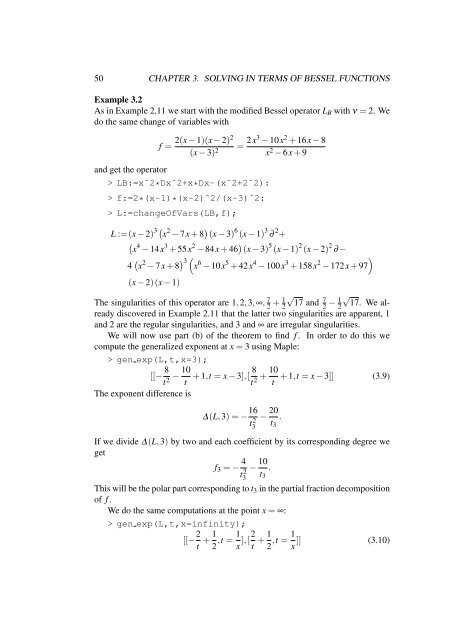
50 CHAPTER 3. SOLVING IN TERMS OF BESSEL FUNCTIONS Example 3.2 As in Example 2.11 we start with the modified Bessel operator LB with ν = 2. We do the same change of variables with f = 2(x − 1)(x − 2)2 (x − 3) 2 and get the operator > LB:=xˆ2*Dxˆ2+x*Dx-(xˆ2+2ˆ2): > f:=2*(x-1)*(x-2)ˆ2/(x-3)ˆ2: > L:=changeOfVars(LB,f); = 2x3 − 10x 2 + 16x − 8 x 2 − 6x + 9 L :=(x − 2) 3 x 2 − 7x + 8 (x − 3) 6 (x − 1) 3 ∂ 2 + 4 3 2 5 2 2 x − 14x + 55x − 84x + 46 (x − 3) (x − 1) (x − 2) ∂− 4 x 2 3 − 7x + 8 x 6 − 10x 5 + 42x 4 − 100x 3 + 158x 2 − 172x + 97 (x − 2)(x − 1) The singularities of this operator are 1,2,3,∞, 7 2 + 1 √ 7 2 17 and 2 − 1 √ 2 17. We already discovered in Example 2.11 that the latter two singularities are apparent, 1 and 2 are the regular singularities, and 3 and ∞ are irregular singularities. We will now use part (b) of the theorem to find f . In order to do this we compute the generalized exponent at x = 3 using Maple: > gen exp(L,t,x=3); [[− 8 10 8 10 − + 1,t = x − 3],[ + + 1,t = x − 3]] (3.9) t2 t t2 t The exponent difference is ∆(L,3) = − 16 t 2 3 − 20 . t3 If we divide ∆(L,3) by two and each coefficient by its corresponding degree we get f3 = − 4 t 2 3 − 10 . t3 This will be the polar part corresponding to t3 in the partial fraction decomposition of f . We do the same computations at the point x = ∞: > gen exp(L,t,x=infinity); [[− 2 t 1 1 + ,t = 2 x ],[2 t + 1 2 1 ,t = ]] (3.10) x
3.1. CHANGE OF VARIABLES 51 ⇒ ∆(L,∞) = − 4t −1 ∞ . Hence, f∞ = −2t −1 ∞ = −2x is the polar part corresponding to t∞. Maple’s output in (3.9) and (3.10) is not ordered. Therefore, we defined ∆ modulo a factor −1. So, we don’t know whether the coefficients of f3 and f∞ are 1 or −1 and we also don’t know the constant part of f . But from the polar parts f3 and f∞ we get candidates for the parameter of the change of variables modulo some constant. The solution must be among those candidates. We also know that the regular singularities 1 and 2 must be zeros of f . So we compute: f3 + f∞| x=1 = 6, f3 + f∞| x=2 = 10, f3 − f∞| x=1 = 2, f3 − f∞| x=2 = 2. We do not need the candidates − f3 + f∞ and − f3 − f∞ since LB −x −→C LB. In other words, if we find a solution where ˜f is the parameter of the change of variables, we will also find a solution if we take the parameter − ˜f in the change of variables. In the first candidate f3 + f∞ we would need two different constants in order to make both x = 1 and x = 2 a zero of f . So the only candidate that remains is ˜f = f3 − f∞ − 2 = − 4 10 − (x − 3) 2 x − 3 − 2x − 2 = −2 x3 − 5x2 + 8x − 4 (x − 3) 2 which, in fact, is equal to − f . As a result we can represent the solutions of L with the modified Bessel functions I2( ˜f ) and K2( ˜f ). At the end of the last chapter we defined exp-apparent points. These are singularities p of an operator L where ∆(L, p) ∈ Z and the solutions at p are not logarithmic. We will now distinguish between two more cases which will correspond to zeros and poles of f . Definition 3.3 Let p be a singularity of the operator L ∈ K[∂] which is not expapparent. Then p is called (i) exp-regular ⇔ ∆(L, p) ∈ C, (ii) exp-irregular ⇔ ∆(L, p) ∈ C[1/tp]\C. We denote the set of singularities that are exp-regular by Sreg and those that are exp-irregular by Sirr.
Page 1 and 2: Solving Differential Equations in T
Page 3 and 4: Contents List of Notations v Introd
Page 5 and 6: List of Notations This is a list of
Page 7 and 8: Introduction Ordinary differential
Page 9 and 10: 1 Preliminaries We will first intro
Page 11 and 12: 1.2. SINGULAR POINTS 11 A linear di
Page 13 and 14: 1.3. HYPERGEOMETRIC SERIES 13 Theor
Page 15 and 16: 1.3. HYPERGEOMETRIC SERIES 15 1.3.1
Page 17 and 18: 1.3. HYPERGEOMETRIC SERIES 17 Remar
Page 19 and 20: 1.4. FORMAL SOLUTIONS AND GENERALIZ
Page 27 and 28: 2 Transformations From now on we wi
Page 29 and 30: 2.1. OPERATORS OF DEGREE TWO 29 in
Page 31 and 32: 2.1. OPERATORS OF DEGREE TWO 31 r 3
Page 33 and 34: 2.1. OPERATORS OF DEGREE TWO 33 The
Page 35 and 36: 2.1. OPERATORS OF DEGREE TWO 35 The
Page 37 and 38: 2.2. THE EXPONENT DIFFERENCE 37 > g
Page 39 and 40: 2.2. THE EXPONENT DIFFERENCE 39 whe
Page 41 and 42: 2.3. EQUIVALENCE OF DIFFERENTIAL OP
Page 47 and 48: 3 Solving in Terms of Bessel Functi
Page 49: 3.1. CHANGE OF VARIABLES 49 We star
Page 53 and 54: 3.2. FINDING THE PARAMETER ν 53 Ex
Page 55 and 56: 3.2. FINDING THE PARAMETER ν 55 If
Page 57 and 58: 3.3. THE ALGORITHM 57 3.3 The Algor
Page 59 and 60: 3.3. THE ALGORITHM 59 Example 3.12
Page 61 and 62: 3.3. THE ALGORITHM 61 > gen exp(L,t
Page 63 and 64: 3.3. THE ALGORITHM 63 We can also f
Page 65 and 66: 3.3. THE ALGORITHM 65 > equiv(L,M);
Page 67 and 68: 3.3. THE ALGORITHM 67 must be a mul
Page 69 and 70: 3.3. THE ALGORITHM 69 2. Let ai,bi
Page 71 and 72: 3.3. THE ALGORITHM 71 The exp-regul
Page 73 and 74: 3.4. SOLVING OVER A GENERAL FIELD K
Page 81 and 82: 3.5. WHITTAKER FUNCTIONS 81 At x =
Page 83 and 84: 3.6. TWO FINAL EXAMPLES 83 > LW:=D
Page 85 and 86: 3.6. TWO FINAL EXAMPLES 85 Since Wh
Page 87 and 88: 4 Conclusion We developed an algori
Page 89 and 90: A Appendix A.1 Transformations From
Page 91 and 92: A.3. PACKAGE DESCRIPTION 91 coeffic
Page 93 and 94: A.3. PACKAGE DESCRIPTION 93 findWhi
Page 95 and 96: Bibliography [1] ABRAMOV, S. A., BA
Page 97 and 98: BIBLIOGRAPHY 97 [23] VAN HOEIJ, M.
Page 99 and 100: Index adjoint operator, 42, 44 alge

Solving Differential Equations in Terms of Bessel Functions

Create successful ePaper yourself

Delete template?

Save as template?