Dye Separation - Leica Microsystems
Dye Separation - Leica Microsystems
Dye Separation - Leica Microsystems

Create successful ePaper yourself
Turn your PDF publications into a flip-book with our unique Google optimized e-Paper software.
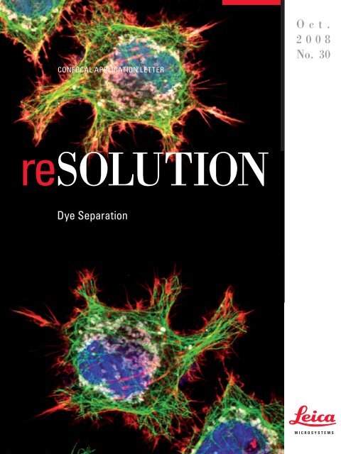
CONFOCAL APPLICATION LETTER<br />
reSOLUTION<br />
<strong>Dye</strong> <strong>Separation</strong><br />
Oct.<br />
2008<br />
No. 30
2 Confocal Application Letter<br />
Introduction<br />
Today a wide variety of fl uorescent dyes and<br />
fl uorescent proteins are available for multicolor<br />
fl uorescence microscopy. Recorded signals from<br />
these fl uorescent molecules provide complex<br />
information about multilabeled samples, often<br />
necessitating quantifi cation or localization/colocalization<br />
analysis.<br />
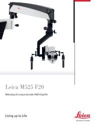
If signifi cant overlap of the excitation or emission<br />
spectra of multiple fl uorophores occurs it becomes<br />
diffi cult to distinguish between the different<br />
signals. Consider a combination of the four<br />
fl uorophores Alexa 488, Alexa 546, Alexa 568 and<br />
TOTO-3 (see Fig. 1). It is diffi cult to separate emission<br />
signals from these dyes due to their strong<br />
spectral overlap, which results in signals from<br />
multiple dyes in each channel. This phenomenon<br />
is termed crosstalk, or bleed-through. Interpreting<br />
multicolor images can be challenging in this<br />
case because they arise from a mixture of signals<br />
from multiple dyes.<br />
Crosstalk<br />
There are different options to avoid and/or remove<br />
crosstalk of fl uorophores for multi-labeled<br />
samples.<br />
For example, when using simultaneous scan<br />
mode there are acquisition strategies to minimize<br />
crosstalk. One way is to optimize the detection<br />
range to avoid crosstalk. Reducing the<br />
excitation light for each respective fl uorophore<br />
will also reduce the emission intensity, which in<br />
turn reduces the degree of crosstalk. But, if the<br />
degree of overlap is too strong (Alexa 546/Alexa<br />
568 or Dapi/FITC) it is better to choose the sequential<br />
scan mode.<br />
However, sequential scan may not be the best<br />
choice when speed is important (i.e. for live cell<br />
imaging). Simultaneous detection of all dyes may<br />
be necessary; sequential scan mode may be too<br />
slow. In addition, samples that are stained with<br />
multiple fl uorophores that are excited by the<br />
Excitation Spectra<br />
400 450 500 550 600 650 700<br />
Emission Spectra<br />
450 500 550 600 650 700 750<br />
Fig.1: Excitation and emission spectra of Alexa 488,<br />
Alexa 546, Alexa 568 and TOTO-3.<br />
same laser line (see example Fig. 1) will exhibit<br />
crosstalk despite using sequential scan. In these<br />
cases a mathematical restoration of dyes into<br />
separate channels may be necessary. This will<br />
be discussed in the following.<br />
Consider a FITC/TRITC double-labeled sample.<br />
See in Fig. 2a the emission spectrum of only one<br />
dye. The total emission light collected from FITC<br />
will be distributed in both channels. Here the<br />
green channel collects about 3/4 of the entire<br />
green signal while 1/4 of the signal spills over into<br />
the red channel.<br />
For the red channel a similar situation exists (Fig.<br />
2b). The total light collected from TRITC will be<br />
distributed in both channels. Here we estimate<br />
4/5 of the red signal is seen in the red channel and<br />
1/5 of the signal goes into the green channel.
Fig. 2a: Emission spectrum of the green channel<br />
We estimate here:<br />
3/4 of all FITC emission goes into the green channel<br />
1/4 of all FITC emission goes into the red channel<br />
Fig. 2b: Emission spectrum of the red channel<br />
We estimate here:<br />
1/5 of all TRITC emission goes into the green channel<br />
4/5 of all TRITC emission goes into the red channel<br />
In a double-stained sample (Fig. 2c), signals from both dyes will be present. In our example you will<br />
record 3/4 FITC + 1/5 TRITC in the green channel and 1/4 FITC + 4/5 TRITC in the red channel.<br />
Fig. 2c: Emission signals of a double-labeled sample. The black curve represents the sum of the signals of both fl uorophores.<br />
Fig. 2d: Removing crosstalk:<br />
1/4 of all FITC emission has to be removed from red channel<br />
1/5 of all TRITC emission has to be removed from green channel<br />
<strong>Dye</strong> <strong>Separation</strong><br />
Confocal Application Letter 3
4 Confocal Application Letter<br />
The goal is now to separate the signals, so that<br />
each channel contains only the signal from one<br />
dye. This means that 1/5 of the TRITC signal has to<br />
be removed from the green channel, and 1/4 of the<br />
FITC signal has to be removed and redistributed<br />
Green channel:<br />
Red channel:<br />
There are different options to fi nd these coeffi -<br />
cients to solve this mathematical problem:<br />
• you may use reference measurements<br />
➔ Channel + Spectral <strong>Dye</strong> <strong>Separation</strong> tool<br />
1. <strong>Dye</strong> <strong>Separation</strong>: Background<br />
<strong>Dye</strong> <strong>Separation</strong> Based on Linear Unmixing<br />
The Linear Unmixing method was initially developed<br />
for processing multiband satellite images.<br />
In general the algorithm is based on the following<br />
assumption: the total emission signal S of<br />
every channel λ is expressed as a linear combination<br />
of the contributing dyes FluoX. A x represents<br />
the amount of contribution by a specifi c<br />
fl uorophore.<br />
from the red channel. The resulting image will be<br />
free of crosstalk (Fig. 2d).<br />
Expressed in mathematical terms you will have<br />
two equations with two unknowns:<br />
• you may estimate the coeffi cients and<br />
subtract crosstalk manually<br />
➔ Manual <strong>Dye</strong> <strong>Separation</strong> tool<br />
• you may use computation through statistical<br />
analysis (Intensity Correlation)<br />
➔ Automatic <strong>Dye</strong> <strong>Separation</strong> tool<br />
This method uses spectral signatures (emission<br />
spectra) as references. In the case of multi-fl uorescence<br />
images, even combined and mixed<br />
emission signals can be clearly separated into<br />
the dyes that contribute to the total signal.<br />
In other words, the system calculates the distribution<br />
coeffi cients of all the dyes in the different<br />
channels.<br />
S(λ) = A 1 x Fluo1(λ) + A 2 x Fluo2(λ) + A 3 x Fluo3(λ)...
1.1 Channel <strong>Dye</strong> <strong>Separation</strong> 1.2 Spectral <strong>Dye</strong> <strong>Separation</strong><br />
For correct unmixing it is necessary to fi nd regions<br />
with pure dyes in the sample as references. The<br />
best way to do this is to use controls that contain<br />
only one of the dyes. This approach reduces the<br />
risk of taking spectra with slight contributions<br />
of other fl uorophores as references. However,<br />
multi-labeled samples may also be used if there<br />
are areas within the specimen that clearly contain<br />
single dye regions without colocalization.<br />
The distribution coeffi cients will be measured,<br />
and the sample can be analyzed. If you need to<br />
separate n different dyes, it is suffi cient to collect<br />
n different channels; no ‘spectrum’ must be<br />
recorded.<br />
General information:<br />
Autofl uorescence<br />
Autofl uorescence of cells may be a signifi -<br />
cant problem in fl uorescence microscopy. By<br />
means of the Channel and Spectral <strong>Dye</strong> <strong>Separation</strong><br />
tool you can treat autofl uorescence as<br />
another fl uorophore (unstained sample as reference)<br />
and thus remove it from the specimenspecifi<br />
c signal.<br />
In the same way background may be removed,<br />
assuming the background of the sample is homogenous.<br />
<strong>Separation</strong> of non-balanced fl uorophores<br />
Sometimes the emissions of different fl uorophores<br />
are not well balanced in intensities. In<br />
this case a weak signal may be partially overlaid<br />
by the crosstalk coming from a strong signal.<br />
With the <strong>Dye</strong> <strong>Separation</strong> tool it is possible to<br />
separate both fl uorophores.<br />
This method is preferred for lambda stacks.<br />
Mathematically it is the same equation used for<br />
the Channel <strong>Dye</strong> <strong>Separation</strong>. Here, the set of<br />
coeffi cients for a dye is the ‘spectrum’.<br />
This method requires the appropriate reference<br />
spectra, which can be measured with a Lambda<br />
scan or which can be taken from the literature.<br />
The spectra can be stored in a spectra database.<br />
<strong>Separation</strong> of fl uorophores excited<br />
with one laser line<br />
Even if your sample is stained with two dyes<br />
excited by the same laser line, the <strong>Dye</strong> <strong>Separation</strong><br />
tool can successfully separate the two fl uorophores.<br />
For example, a sample containing<br />
both Alexa 488 and GFP requires 488 nm light<br />
for excitation of both fl uorophores. As mentioned<br />
above, a sequential scan will not eliminate<br />
crosstalk in this example. However, even<br />
though the emission spectra extremely overlap,<br />
it is still possible to separate the signals using<br />
reference samples.<br />
Note: The Spectral <strong>Dye</strong> <strong>Separation</strong> tool cannot<br />
be used in the special case where the fl uorophores<br />
are both excited by a single laser line<br />
AND their intensities are signifi cantly different.<br />
<strong>Dye</strong> <strong>Separation</strong><br />
Confocal Application Letter 5
6 Confocal Application Letter<br />
1.3 Manual <strong>Dye</strong> <strong>Separation</strong><br />
In the Manual tool the distribution coeffi cients<br />
are not calculated by the system but are estimated<br />
by the user, i.e. no references are needed. Let’s<br />
explain it using the example described above.<br />
To get crosstalk-free images we estimate that 1/5<br />
of the TRITC signal has to be removed from the<br />
green channel and 1/4 FITC signal has to be removed<br />
from the red channel. The user only needs<br />
to apply the estimated numbers to a matrix.<br />
Note: If your system is equipped with the Colocalization<br />
Analysis tool (license is required), you<br />
can use the cytofl uorogram to get the coeffi -<br />
cients (see page 22).<br />
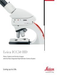
<strong>Dye</strong> <strong>Separation</strong> based on Intensity Correlation<br />
The <strong>Leica</strong> Automatic <strong>Dye</strong> <strong>Separation</strong> (Weak &<br />
Strong) software analyses the correlation of the<br />
grey values of the pixels in different channels. A<br />
scatter plot known as a cytofl uorogram represents<br />
such correlations and is used for example<br />
in colocalization analysis.<br />
The cytofl uorogram (Fig. 3) shows grey values<br />
of channels one and two on the x- and y-axis,<br />
respectively. Each pixel in the scatter plot represents<br />
an intensity pair (green-red) of the original<br />
detection channels. Crosstalk of the green<br />
dye into the red channel is defi ned by the angle<br />
of the data cloud with the x-axis (0° defi ning 0%<br />
crosstalk). In the same manner, crosstalk of the<br />
red dye into the green channel is defi ned by the<br />
angle of the data cloud with the y-axis.<br />
Fig. 3: Cytofl uorogram shows the intensity relationships<br />
between two channels.
1.4 Automatic <strong>Dye</strong> <strong>Separation</strong>: Weak and Strong<br />
The Automatic <strong>Dye</strong> <strong>Separation</strong> tool uses a mathematical<br />
procedure, called cluster analysis, for<br />
classifying objects into homogenous groups. In<br />
our case the objects being classifi ed are the<br />
grey values of the pixels, which are acquired in<br />
different detection channels.<br />
After identifying clusters of homogenous image<br />
data, the best-fi t line for the clouds in the cytofl<br />
uogram is determined. Crosstalk correction is<br />
achieved by ‘moving’ the fi tted clouds to the axes<br />
(Fig. 4a–4d). The advantage of this method is that<br />
no spectral information is needed – the main distributions<br />
are found by fi tting.<br />
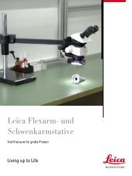
The Automatic <strong>Dye</strong> <strong>Separation</strong><br />
(Weak & Strong)<br />
methods will move the<br />
clouds to the axes.<br />
Fig. 4a: Ideal separation of<br />
fl uorescent signals, without<br />
crosstalk; each channel<br />
is related to its own dye.<br />
Fig. 4b: Fluorescent signals<br />
if crosstalk occurs: the<br />
clouds are tilted towards<br />
the diagonal.<br />
Fig. 4c:<br />
Correction of crosstalk<br />
Fig. 4d: After processing:<br />
Ideal separation of fl uorescent<br />
signals, each channel<br />
is related to its own dye.<br />
<strong>Dye</strong> <strong>Separation</strong><br />
Confocal Application Letter 7
8 Confocal Application Letter<br />
What is the difference between Weak and Strong <strong>Dye</strong> <strong>Separation</strong>?<br />
Weak:<br />
Strong:<br />
The weak method of Automatic<br />
<strong>Dye</strong> <strong>Separation</strong> will<br />
move the clouds until they<br />
just touch the axes.<br />
The strong method of Automatic<br />
<strong>Dye</strong> <strong>Separation</strong><br />
will move the clouds to coincide<br />
with the axes.
2. <strong>Dye</strong> <strong>Separation</strong>: Choosing the Right Tool<br />
Channel <strong>Dye</strong> <strong>Separation</strong><br />
• When pure dyes are present in the sample<br />
or references are available<br />
• For separation of two fl uorophores with strong<br />
emission overlap, excited with the same<br />
excitation line<br />
• For separation of autofl uorescence<br />
Spectral <strong>Dye</strong> <strong>Separation</strong><br />
• When reference spectra are available<br />
• For lambda-series<br />
• For separation of autofl uorescence<br />
Manual <strong>Dye</strong> <strong>Separation</strong><br />
• When no reference spectra are available<br />
• When Automatic <strong>Dye</strong> <strong>Separation</strong> (see below)<br />
have failed<br />
3. <strong>Dye</strong> <strong>Separation</strong> in LAS AF<br />
You can fi nd the <strong>Dye</strong> <strong>Separation</strong> tool under Process<br />
➀ and the tab Tools ➁.<br />
➀<br />
➁<br />
Select the Channel <strong>Dye</strong> <strong>Separation</strong> tool. To determine<br />
the distribution coeffi cients of the fl uorophores<br />
(i.e. degree of crosstalk) you need to<br />
defi ne reference regions within your image or<br />
series. You may use multi-labeled samples with<br />
pure dye regions (see paragraph A). Reference<br />
regions may also be defi ned on separately acquired<br />
single-dye control images (see paragraph<br />
B). Note that you have to keep detection parameters<br />
identical for the reference images.<br />
Automatic <strong>Dye</strong> <strong>Separation</strong>: Weak & Strong<br />
• When no reference spectra are available;<br />
precondition: good signal to noise ratio<br />
• Weak method: weak background<br />
and noise reduction<br />
• Strong method: strong background<br />
and noise reduction<br />
3.1 Channel <strong>Dye</strong> <strong>Separation</strong>: Step by Step<br />
In order to get reasonable results with any of the<br />
<strong>Dye</strong> <strong>Separation</strong> tools, it is important to have images<br />
with good signal to noise ratios.<br />
<strong>Dye</strong> <strong>Separation</strong><br />
Confocal Application Letter 9
10 Confocal Application Letter<br />
A. When pure dye in a multi-labeled sample is present<br />
1. Place the crosshair in the viewer ➀ to a position that clearly contains a single dye.<br />
You can also draw a ROI manually after activating the ROI function in the viewer ➁.<br />
➁<br />
➀<br />
Bovine pulmonary artery endothelial cells (BPAEC); green: BODIPY FL phallacidin, F-actin; red: MitoTracker Red CMXRos,<br />
mitochondria.<br />
Note: If there is no crosshair visible in the viewer you can activate it by clicking on the Crosshair<br />
button .<br />
2. In the fi eld Measurement Area ➂ you may adjust the size of the reference region (in voxels).<br />
➂
The histogram visualizes the color distribution inside of the reference region.<br />
3. Click Add ➃ to defi ne the chosen position as a reference region to determine the<br />
distribution coeffi cients of this fl uorescent dye.<br />
Every reference region you defi ne is added to the list box ➄.<br />
Clear and Clear all ➅ delete a marked reference or all references, respectively.<br />
➄<br />
➃<br />
➅ ➆<br />
4. Repeat steps 1-3 for all dyes used in your image.<br />
5. Choose a method of rescaling ➆ for the resulting images or series.<br />
<strong>Dye</strong> <strong>Separation</strong><br />
Confocal Application Letter 11
12 Confocal Application Letter<br />
There are two options for rescaling:<br />
Per Channel: All channels are rescaled separately to spread the dynamic range of the images over<br />
the entire range of bit depth (e.g. 8 bit from 0 to 255). This operation results in brighter images, but<br />
these images cannot be further quantifi ed.<br />
All Channels: All channels are rescaled together using the same factor, thereby maintaining the proportion.<br />
In this case only one channel gets the maximum bit depth.<br />
6. Click Apply ➇ to perform the image processing.<br />
To preview the changes, press the Preview button. The Reset function allows you to go back to the<br />
default settings.<br />
Original image with crosstalk<br />
Channel_<strong>Dye</strong>_<strong>Separation</strong>_image_crosstalk.tif<br />
B. Using reference images<br />
Resulting image without crosstalk<br />
If you want to use control images of single labeled specimens as reference samples, you must capture<br />
all of the images using the same detection parameters that were chosen for the multi-labeled sample.<br />
1. Select the fi rst single-dye control image in the experiment tab ➀.<br />
➀<br />
➇
2. Place the crosshair in the viewer ➁ to an appropriate position.<br />
You can also draw a ROI manually.<br />
➁<br />
HeLa cells, reference 1: single-labeled cells imaged using the same conditions as the double-labeled sample; cyan (1. channel):<br />
Dapi, nucleus; green (2. channel): crosstalk of Dapi.<br />
3. Click Add ➂ to defi ne this position.<br />
➂<br />
➄<br />
<strong>Dye</strong> <strong>Separation</strong><br />
Confocal Application Letter 13
14 Confocal Application Letter<br />
4. Select the second single-dye control image in the experiment tab ➃.<br />
5. Place the crosshair in the viewer and again click Add ➂ to defi ne the second coeffi cient.<br />
6. Repeat this process for all of the dyes used.<br />
7. Choose a method of rescaling ➄ for the resulting images (see page 12).<br />
8. Select the images to be unmixed ➅.<br />
9. Click Apply.<br />
➃<br />
HeLa cells, reference 2: single-labeled cells imaged using the same conditions as the double-labeled sample; no signal recorded<br />
in the 1. channel; green (2. channel): Alexa 488, tubulin.<br />
➅
<strong>Separation</strong> of two fl uorophores<br />
Original image with crosstalk<br />
HeLa cells (fi broblasts); blue: Dapi, nucleus, green: Alexa 488, tubulin.<br />
<strong>Separation</strong> of four fl uorophores<br />
Original image with crosstalk<br />
Resulting image without crosstalk<br />
Resulting image without crosstalk<br />
HeLa cells (fi broblasts); blue: Dapi, nucleus; green: Alexa 488, tubulin; red: TRITC phalloidin, actin; grey: Mito Tracker Red<br />
CMXRos, mitochondria.<br />
<strong>Dye</strong> <strong>Separation</strong><br />
Confocal Application Letter 15
16 Confocal Application Letter<br />
3.2 Spectral <strong>Dye</strong> <strong>Separation</strong>: Step by Step<br />
Select the Spectral <strong>Dye</strong> <strong>Separation</strong> tool.<br />
You may unmix by choosing reference spectra from a spectral database (see paragraph A) or you<br />
may add your own measured dye spectra (see paragraph B).<br />
A. Using reference spectra from a database<br />
1. Select the corresponding fl uorophore from the database ➀.<br />
If your image contains multiple fl uorophores click Add ➁ to choose additional spectra.<br />
2. Choose a method of rescaling ➂ (see Channel <strong>Dye</strong> <strong>Separation</strong>, page 12).<br />
3. Click Apply.<br />
➀<br />
➁<br />
B. Using measured reference spectra<br />
1. Place the crosshair ➀ in a region of your choice. You can also draw a ROI manually.<br />
Note: If there is no crosshair visible in the viewer you may activate it by clicking on the<br />
Crosshair button .<br />
➂
2. In the fi eld Measurement Area ➁ you may alter the size of the reference region (in voxels).<br />
3. Click Save Current Spectrum ➂ to add the actual spectrum to the Spectra Database.<br />
➁<br />
➀<br />
➂<br />
<strong>Dye</strong> <strong>Separation</strong><br />
Confocal Application Letter 17
18 Confocal Application Letter<br />
A dialog box will open automatically.<br />
The measured emission spectrum of the fl uorophore is displayed and can be saved in the spectra<br />
database.<br />
➅<br />
➃<br />
➄<br />
➆
4. Fill in the fi elds ➃ accordingly. By clicking on Save ➄ the spectrum is saved under User in the<br />
Table of spectra ➅.<br />
5. Press X ➆ to go back to the Spectral <strong>Dye</strong> <strong>Separation</strong> dialog. The saved spectrum is now available<br />
in the list under User ➇. You may continue as described under paragraph A.<br />
➇<br />
Part of the image gallery of a lambda series of Drosophila melanogaster stained with Alexa 488, Alexa 546, Alexa 568 and TOTO-3.<br />
➅<br />
<strong>Dye</strong> <strong>Separation</strong><br />
Confocal Application Letter 19
20 Confocal Application Letter<br />
Fluorescence signals are separated after processing the spectral data with the Spectral <strong>Dye</strong> <strong>Separation</strong> tool.<br />
Courtesy of Dr. Ralf Pfl anz, MPI Biophysical Chemistry, Göttingen<br />
3.3 Manual <strong>Dye</strong> <strong>Separation</strong><br />
Clicking on Automatic opens a dialog box, where you can choose the settings for either the Manual<br />
<strong>Dye</strong> <strong>Separation</strong> or the Automatic <strong>Dye</strong> <strong>Separation</strong> methods. Choosing Manual opens a new dialog<br />
window.
➀<br />
1. Select the Manual ➀ method in the Automatic <strong>Dye</strong> <strong>Separation</strong> window. A new dialog box opens<br />
that will allow you to unmix the crosstalk of one channel from the other manually.<br />
Note: The fi eld Fluorescent <strong>Dye</strong>s ➁ refl ects the number of dyes used during image acquisition.<br />
LAS AF recognizes this and automatically displays the number of channels.<br />
2. Choose a method of rescaling ➂ the resulting images or series (see Channel <strong>Dye</strong> <strong>Separation</strong>,<br />
page 12).<br />
3. Type the desired coeffi cients into the matrix fi elds ➃. In this example we correct 1/3 cross-talk<br />
from the green dye in the red channel and 1/10 cross-talk from the red dye in the green channel.<br />
The matrix can be saved and reloaded ➄ for reproducibility. Keep in mind that in order to<br />
use the same contribution coeffi cients in the matrix, identical recordings using the same<br />
parameters must be taken.<br />
The Reset Matrix ➅ button allows you to go back to the default settings.<br />
➁<br />
➃<br />
➅ ➄<br />
➂<br />
➆<br />
<strong>Dye</strong> <strong>Separation</strong><br />
Confocal Application Letter 21
22 Confocal Application Letter<br />
4. Close the Edit Matrix dialog ➆ (see page 21) and click Apply ➇.<br />
Note: 1. The Edit Matrix button is active only if you have selected the Manual option under Method.<br />
2. Lambda scans cannot be processed with the Automatic <strong>Dye</strong> <strong>Separation</strong> tool.<br />
If the Colocalization tool is available on your system, you can use the cytofl uorogram to determine<br />
the coeffi cients. By defi ning the threshold for both channels you can obtain a best-fi t line for the<br />
clouds. In this example the coeffi cients are 0.35 for channel 1 and 0.05 for channel 2 (see explanation<br />
under Automatic <strong>Dye</strong> <strong>Separation</strong>: Weak and Strong, page 6ff)<br />
➇
3.4 Automatic <strong>Dye</strong> <strong>Separation</strong>: Weak and Strong<br />
Choose the Automatic <strong>Dye</strong> <strong>Separation</strong> tool.<br />
➀<br />
1. Select between method Weak or Strong ➀.<br />
➁<br />
Note: The fi eld Fluorescent <strong>Dye</strong>s ➁ refl ects the number of dyes used during image acquisition.<br />
LAS AF recognizes this and automatically displays the number of channels.<br />
2. Choose a method of rescaling ➂ the resulting images or series (see Channel <strong>Dye</strong> <strong>Separation</strong>,<br />
page 12).<br />
➄ ➅ ➃<br />
3. Apply ➃ transfers the unmixed data fi le to Experiments.<br />
To preview the changes, press the Preview ➄ button. The Reset ➅ function allows you to go<br />
back to the default settings.<br />
References:<br />
F. Olschewski, Living Colors, Excellent Solutions for Live Cell Imaging, G.I.T. Imaging & Microscopy 2/2002<br />
T. Zimmermann, Spectral Imaging and Linear Unmixing in Light Microscopy, Adv Biochem Eng Biotechnol. 2005;95:245-65<br />
➂<br />
<strong>Dye</strong> <strong>Separation</strong><br />
Confocal Application Letter 23
“With the user, for the user”<br />
<strong>Leica</strong> <strong>Microsystems</strong><br />
<strong>Leica</strong> <strong>Microsystems</strong> operates internationally in four divisions,<br />
where we rank with the market leaders.<br />
• Life Science Division<br />
The <strong>Leica</strong> <strong>Microsystems</strong> Life Science Division supports the<br />
imaging needs of the scientifi c community with advanced<br />
innovation and technical expertise for the visualization,<br />
measurement, and analysis of microstructures. Our strong<br />
focus on understanding scientifi c applications puts <strong>Leica</strong><br />
<strong>Microsystems</strong>’ customers at the leading edge of science.<br />
• Industry Division<br />
The <strong>Leica</strong> <strong>Microsystems</strong> Industry Division’s focus is to<br />
support customers’ pursuit of the highest quality end result.<br />
<strong>Leica</strong> <strong>Microsystems</strong> provide the best and most innovative<br />
imaging systems to see, measure, and analyze the microstructures<br />
in routine and research industrial applications,<br />
materials science, quality control, forensic science investigation,<br />
and educational applications.<br />
• Biosystems Division<br />
The <strong>Leica</strong> <strong>Microsystems</strong> Biosystems Division brings histopathology<br />
labs and researchers the highest-quality,<br />
most comprehensive product range. From patient to pathologist,<br />
the range includes the ideal product for each<br />
histology step and high-productivity workfl ow solutions<br />
for the entire lab. With complete histology systems featuring<br />
innovative automation and Novocastra reagents,<br />
<strong>Leica</strong> <strong>Microsystems</strong> creates better patient care through<br />
rapid turnaround, diagnostic confi dence, and close customer<br />
collaboration.<br />
• Surgical Division<br />
The <strong>Leica</strong> <strong>Microsystems</strong> Surgical Division’s focus is to<br />
partner with and support surgeons and their care of patients<br />
with the highest-quality, most innovative surgi cal<br />
microscope technology today and into the future.<br />
www.leica-microsystems.com<br />
The statement by Ernst Leitz in 1907, “with the user, for the user,” describes the fruitful collaboration<br />
with end users and driving force of innovation at <strong>Leica</strong> <strong>Microsystems</strong>. We have developed fi ve<br />
brand values to live up to this tradition: Pioneering, High-end Quality, Team Spirit, Dedication to<br />
Science, and Continuous Improvement. For us, living up to these values means: Living up to Life.<br />
Active worldwide<br />
Australia: North Ryde Tel. +61 2 8870 3500 Fax +61 2 9878 1055<br />
Austria: Vienna Tel. +43 1 486 80 50 0 Fax +43 1 486 80 50 30<br />
Belgium: Groot Bijgaarden Tel. +32 2 790 98 50 Fax +32 2 790 98 68<br />
Canada: Richmond Hill/Ontario Tel. +1 905 762 2000 Fax +1 905 762 8937<br />
Denmark: Herlev Tel. +45 4454 0101 Fax +45 4454 0111<br />
France: Rueil-Malmaison Tel. +33 1 47 32 85 85 Fax +33 1 47 32 85 86<br />
Germany: Wetzlar Tel. +49 64 41 29 40 00 Fax +49 64 41 29 41 55<br />
Italy: Milan Tel. +39 02 574 861 Fax +39 02 574 03392<br />
Japan: Tokyo Tel. +81 3 5421 2800 Fax +81 3 5421 2896<br />
Korea: Seoul Tel. +82 2 514 65 43 Fax +82 2 514 65 48<br />
Netherlands: Rijswijk Tel. +31 70 4132 100 Fax +31 70 4132 109<br />
People’s Rep. of China: Hong Kong Tel. +852 2564 6699 Fax +852 2564 4163<br />
Portugal: Lisbon Tel. +351 21 388 9112 Fax +351 21 385 4668<br />
Singapore Tel. +65 6779 7823 Fax +65 6773 0628<br />
Spain: Barcelona Tel. +34 93 494 95 30 Fax +34 93 494 95 32<br />
Sweden: Kista Tel. +46 8 625 45 45 Fax +46 8 625 45 10<br />
Switzerland: Heerbrugg Tel. +41 71 726 34 34 Fax +41 71 726 34 44<br />
United Kingdom: Milton Keynes Tel. +44 1908 246 246 Fax +44 1908 609 992<br />
USA: Bannockburn/lllinois Tel. +1 847 405 0123 Fax +1 847 405 0164<br />
and representatives in more than 100 countries<br />
Order no.: 1593104017<br />
LEICA and the <strong>Leica</strong> Logo are registered trademarks of <strong>Leica</strong> IR GmbH.