Recurrence equations and their classical orthogonal polynomial ...

More documents

Recommendations

Info

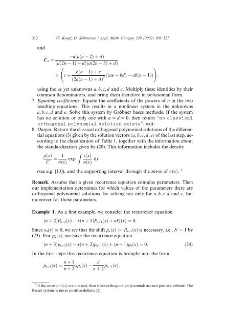
312 W. Koepf, D. Schmersau / Appl. Math. Comput. 128 (2002) 303–327 and eCn ¼ ðað2n nðaðn 2ÞþdÞ 1ÞþdÞðað2n 3ÞþdÞ ! bðn c þ ð2aðn 1Þþe ððae 2 1ÞþdÞ bdÞ abðn 1ÞÞ ; using the as yet unknowns a; b; c; d and e. Multiply these identities by their common denominators, and bring them therefore in polynomial form. 7. Equating coefficients: Equate the coefficients of the powers of n in the two resulting equations. This results in a nonlinear system in the unknowns a; b; c; d and e. Solve this system by Gr€obner bases methods. If the system has no solution or only one with a ¼ d ¼ 0, then return ‘‘no classical orthogonal polynomial solution exists’’; exit. 8. Output: Return the classical orthogonal polynomial solutions of the differential equations (3) given by the solution vectors ða; b; c; d; eÞ of the last step, according to the classification of Table 1, together with the information about the standardization given by (20). This information includes the density qðxÞ 1 ¼ C rðxÞ exp Z sðxÞ rðxÞ dx (see e.g. [13]), and the supporting interval through the zeros of rðxÞ. 1 Remark. Assume that a given recurrence equation contains parameters. Then our implementation determines for which values of the parameters there are orthogonal polynomial solutions, by solving not only for a; b; c; d and e, but moreover for those parameters. Example 1. As a first example, we consider the recurrence equation ðn þ 2ÞPnþ2ðxÞ xðn þ 1ÞPnþ1ðxÞþnPnðxÞ ¼0: Since s0ðxÞ 0, we see that the shift pnðxÞ :¼ Pnþ1ðxÞ is necessary, i.e., N ¼ 1by (23). For pnðxÞ, we have the recurrence equation ðn þ 3Þpnþ2ðxÞ xðn þ 2Þpnþ1ðxÞþðn þ 1ÞpnðxÞ ¼0: ð24Þ In the first steps this recurrence equation is brought into the form pnþ1ðxÞ ¼ n þ 1 n þ 2 xpnðxÞ n n þ 2 pn 1ðxÞ; 1 If the zeros of rðxÞ are not real, then these orthogonal polynomials are not positive-definite. The Bessel system is never positive-definite [2].
hence An ¼ knþ1 kn and therefore ¼ n þ 1 vn ¼ ; n þ 2 wn kn ¼ 1 n þ 1 k0: Moreover, for monic ep nðxÞ ¼pnðxÞ=kn we get ep nþ1ðxÞ ¼xep nðxÞþep n 1ðxÞ; hence eBn ¼ 0and e Cn ¼ 1. The polynomial identities concerning eBn and e Cn of step 5 of the algorithm yield b ¼ 0, c ¼ 4a, and either d ¼ a; or d ¼ 2a; or d ¼ 3a: At this point we have already determined rðxÞ ¼ax 2 þ bx þ c ¼ aðx 2 4Þ: Hence possible classical orthogonal polynomial solutions of (24) are defined in the interval ½ 2; 2Š. In the first of the above cases, i.e., for d ¼ a, one gets e ¼ 0 and the differential equation ðx 2 W. Koepf, D. Schmersau / Appl. Math. Comput. 128 (2002) 303–327 313 4Þy 00 ðxÞþxy 0 ðxÞ corresponding to the density nðn 2ÞyðxÞ ¼0 ð25Þ qðxÞ ¼ 1 rðxÞ exp Z sðxÞ 1 dx ¼ ffiffiffiffiffiffiffiffiffiffiffiffi rðxÞ 4 x2 p : The corresponding orthogonal polynomials are multiples of translated Chebyshev polynomials of the first kind pnðxÞ ¼knCnðxÞ ¼ p0 n þ 1 CnðxÞ ¼ 2p0 n þ 1 Tnðx=2Þ ðnP0Þ ð26Þ (see e.g. [1], Table 22.2, and (22.5.11); CnðxÞ are monic, but C0 ¼ 2, see also Table 22.7), hence finally PnðxÞ ¼pn 1ðxÞ ¼ 2P1 n Tn 1ðx=2Þ ðnP1Þ: In the second of the above cases, i.e., for d ¼ 2a, one gets the equation a 2 ðe 2aÞðe þ 2aÞ ¼0
Page 1 and 2: Recurrence equations and their clas
Page 3 and 4: W. Koepf, D. Schmersau / Appl. Math
Page 5 and 6: and kn 1 Cn ¼ knþ1 ðd ðan þ d
Page 7 and 8: ðqnðxÞ; rnðxÞ; snðxÞ 2Q½n;
Page 9: If we apply this algorithm to the r
Page 13 and 14: W. Koepf, D. Schmersau / Appl. Math
Page 15 and 16: Table 2 Normal forms of discrete po
Page 17 and 18: knþ1 kn :¼ An ¼ vn wn according
Page 19 and 20: With Koornwinder-Swarttouw’s rec2
Page 21 and 22: Table 3 Normal forms of q-polynomia
Page 23 and 24: according to (14), in terms of the
Page 25: W. Koepf, D. Schmersau / Appl. Math

Recurrence equations and their classical orthogonal polynomial ...

You also want an ePaper? Increase the reach of your titles

Delete template?

Save as template?