Recurrence equations and their classical orthogonal polynomial ...

320 W. Koepf, D. Schmersau / Appl. Math. Comput. 128 (2002) 303–327
sideration since the difference equation (5) is not invariant under those transformations.
This leads to step 4 of the algorithm.
Note that an application of Algorithm 2 to the recurrence equation
pnþ2ðxÞ ðx n 1Þpnþ1ðxÞ ¼0 which is valid for the falling factorial
pnðxÞ ¼x n , generates the difference equation xDrpnðxÞ xDpnðxÞþnpnðxÞ ¼0
of Table 2(2a).
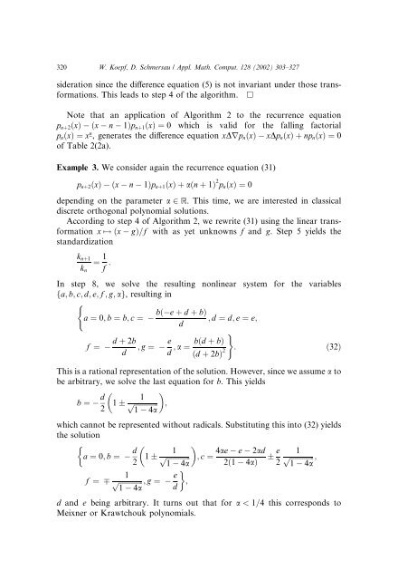
Example 3. We consider again the recurrence equation (31)
pnþ2ðxÞ ðx n 1Þpnþ1ðxÞþaðn þ 1Þ 2 pnðxÞ ¼0
depending on the parameter a 2 R. This time, we are interested in classical
discrete orthogonal polynomial solutions.
According to step 4 of Algorithm 2, we rewrite (31) using the linear transformation
x 7! ðx gÞ=f with as yet unknowns f and g. Step 5 yields the
standardization
knþ1
¼
kn
1
f :
In step 8, we solve the resulting nonlinear system for the variables
fa; b; c; d; e; f ; g; ag, resulting in
(
a ¼ 0; b ¼ b; c ¼
f ¼
d þ 2b
; g ¼
d
bð e þ d þ bÞ
; d ¼ d; e ¼ e;
d
e bðd þ bÞ
; a ¼
d ðd þ 2bÞ 2
)
: ð32Þ
This is a rational representation of the solution. However, since we assume a to
be arbitrary, we solve the last equation for b. This yields
b ¼ d
2 1
1
p ffiffiffiffiffiffiffiffiffiffiffiffiffi ;
1 4a
which cannot be represented without radicals. Substituting this into (32) yields
the solution
a ¼ 0; b ¼ d
2 1
1 4ae e 2ad e 1
p ffiffiffiffiffiffiffiffiffiffiffiffiffi ; c ¼ p ffiffiffiffiffiffiffiffiffiffiffiffiffi ;
1 4a 2ð1 4aÞ 2 1 4a
1
e
f ¼ p ffiffiffiffiffiffiffiffiffiffiffiffiffi ; g ¼ ;
1 4a d
d and e being arbitrary. It turns out that for a < 1=4 this corresponds to
Meixner or Krawtchouk polynomials.