Spatial Characterization Of Two-Photon States - GAP-Optique

1
0
-0.2
1.3. Approximations and other considerations
Gaussian Sine Cardinal
0
FWHM
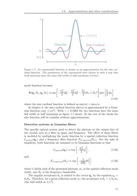
Figure 1.7: An exponential function is chosen as an approximation for the sine cardinal
function. The parameters of the exponential were chosen in such a way that
both functions have the same full width at half maximum (fwhm).
mode function becomes
Φ(q s, Ωs, q i, Ωi) ∝ exp
− w2 p
4 ∆2 0 − w2 p
4 ∆2 1 − T0
4 (Ωs + Ωi) 2
sinc
L
2 ∆k
(1.31)
where the sine cardinal function is defined as sinc(a) = sin a/a.
In chapter 2, the sine cardinal function sinc(a) is approximated by a Gaussian
function exp[−(γa) 2 ]. With γ = 0.4393 the two functions have the same
full width at half maximum as figure 1.7 shows. In the rest of the thesis the
sinc function will be consider without approximations.
Detection systems as Gaussian filters
The specific optical system used to detect the photons at the output face of
the crystal, acts as a filter in space and frequency. The effect of these filters
is modeled by multiplying the mode function by a spatial collection function
Cspatial(qn) and a frequency filter function Ffrequency(Ωn). For the sake of
simplicity, both functions are assumed to be Gaussian functions so that
Cspatial(qn) ∝ exp − w2 n
2 q2
n , (1.32)
and
Ffrequency(Ωn) ∝ exp − 1
2B2 Ω
n
2
n , (1.33)
where n labels each of the generated photons, wn is the spatial collection mode
width, and Bn is the frequency bandwidth.
The angular acceptance θn is related to the vector qn by the equation qn =
knθn. Therefore, for a given collection mode wn the acceptance is θn = 1/knwn
(the half width at 1/e 2 ).
11