Spatial Characterization Of Two-Photon States - GAP-Optique

2. Correlations and entanglement
chosen. In the particular case of a two-photon system, the purity of the spatial
part can be used to study correlations between the degrees of freedom, or the
purity of the signal photon can be used to study the entanglement between the
photons. The next sections explore both these approaches.
2.2 Correlations between space and frequency
In type-i spdc, the photons generated have a polarization orthogonal to the
polarization of the incident beam. Therefore, the two-photon state generated
in a type-i process has only two degrees of freedom: frequency and transversal
spatial distribution. In this section, I study the origin and the characteristics
of the correlations between those degrees of freedom by using the purity of the
spatial part as a correlation indicator.
Except for hyperentanglement configurations [12, 13] and some other novel
configurations [6, 14], most applications of type-i spdc processes use just one of
the degrees of freedom, ignoring the correlation that may exist between space
and frequency. That is, those configurations assume a high degree of spatial
purity. This section explores the conditions in which this assumption is valid.
The first part of this section contains a discussion about the origin and
suppression of the correlations. The second part includes the calculations for
the spatial purity that is used as correlation indicator. The third part shows
the results of numerical calculation of the spatial purity in several cases.
2.2.1 Origin of the correlations
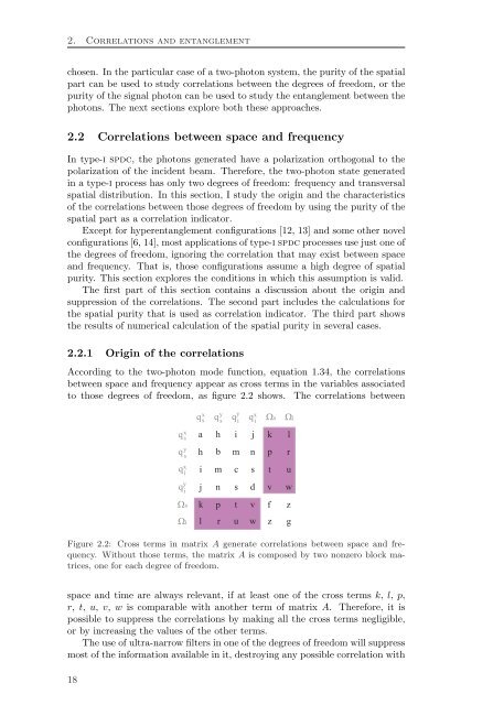
According to the two-photon mode function, equation 1.34, the correlations
between space and frequency appear as cross terms in the variables associated
to those degrees of freedom, as figure 2.2 shows. The correlations between
q s x
q s y
q i x
y
qi s
i
qs x
a
h
i
j
k
l
q s
y
h
b
m
n
p
r
qi y
i
m
c
s
t
u
Figure 2.2: Cross terms in matrix A generate correlations between space and frequency.
Without those terms, the matrix A is composed by two nonzero block matrices,
one for each degree of freedom.
space and time are always relevant, if at least one of the cross terms k, l, p,
r, t, u, v, w is comparable with another term of matrix A. Therefore, it is
possible to suppress the correlations by making all the cross terms negligible,
or by increasing the values of the other terms.
The use of ultra-narrow filters in one of the degrees of freedom will suppress
most of the information available in it, destroying any possible correlation with
18
q i
x
j
n
s
d
v
w
s
k
p
t
v
f
z
i
l
r
u
w
z
g