Spatial Characterization Of Two-Photon States - GAP-Optique
Spatial Characterization Of Two-Photon States - GAP-Optique
Spatial Characterization Of Two-Photon States - GAP-Optique

You also want an ePaper? Increase the reach of your titles
YUMPU automatically turns print PDFs into web optimized ePapers that Google loves.
2.3. Correlations between signal and idler<br />
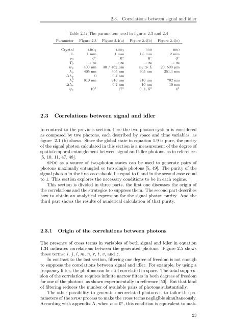
Table 2.1: The parameters used in figures 2.3 and 2.4<br />
Parameter Figure 2.3 Figure 2.4(a) Figure 2.4(b) Figure 2.4(c)<br />
Crystal liio3 liio3 bbo bbo<br />
L 1 mm 1 mm 1.5 mm 2 mm<br />
ρ0 0 ◦ 0 ◦ 0 ◦ 0 ◦<br />
T0 → ∞ → ∞ → ∞ → ∞<br />
wp 400 µm 30 / 462 µm wp ≫ L 20, 500 µm<br />
λp 405 nm 405 nm 405 nm 351.1 nm<br />
∆λp 0 0.4 nm<br />
λ 0 s 810 nm 810 nm 810 nm 702 nm<br />
∆λs 0.2 nm 10 nm 10 nm<br />
ϕs 10 ◦ 17 ◦ 0, 1, 5 ◦ 4 ◦<br />
2.3 Correlations between signal and idler<br />
In contrast to the previous section, here the two-photon system is considered<br />
as composed by two photons, each described by space and time variables, as<br />
figure 2.1 (b) shows. Since the global state in equation 1.9 is pure, the purity<br />
of the signal photon calculated in this section is a measurement of the degree of<br />
spatiotemporal entanglement between signal and idler photons, as in references<br />
[5, 10, 11, 47, 48].<br />
spdc as a source of two-photon states can be used to generate pairs of<br />
photons maximally entangled or two single photons [5, 49]. The purity of the<br />
signal photon in the first case should be equal to 0 and in the second case equal<br />
to 1. This section explores the necessary conditions to be in each regime.<br />
This section is divided in three parts, the first one discusses the origin of<br />
the correlations and the strategies to suppress them. The second part describes<br />
how to obtain an analytical expression for the signal photon purity. And the<br />
third part shows the results of numerical calculation of that purity.<br />
2.3.1 Origin of the correlations between photons<br />
The presence of cross terms in variables of both signal and idler in equation<br />
1.34 indicates correlations between the generated photons. Figure 2.5 shows<br />
those terms: i, j, l, m, n, r, t, v, and z.<br />
In contrast to the last section, filtering one degree of freedom is not enough<br />
to suppress the correlations between signal and idler. For example, by using a<br />
frequency filter, the photons can be still correlated in space. The total suppression<br />
of the correlation requires infinite narrow filters in both degrees of freedom<br />
for one of the photons, as shown experimentally in reference [50]. But that kind<br />
of filtering reduces the number of available pairs of photons substantially.<br />
The other possibility to generate uncorrelated photons is to tailor the parameters<br />
of the spdc process to make the cross terms negligible simultaneously.<br />
According with appendix A, when α = 0 ◦ , this condition is equivalent to mak-<br />
23