Signal Analysis Research (SAR) Group - RNet - Ryerson University

excision blocks in communications.
The paper is organized as follows: Section II describes
the signal and system model, spread spectrum system and
chirp signals. Section III defines the discrete polynomial
phase transform technique. Section IV outlines numerical and
simulation results. And the last Section V is the conclusion
and the summary of the paper.
II. SIGNAL AND SYSTEM MODEL
A. Spread Spectrum System
Assuming Binary Phase Shift Keying modulation (BPSK),
the transmitted spread spectrum signal s(t) consists of the
message signal m(t) and the spreading signal p(t),
where
This full text paper was peer reviewed at the direction of IEEE Communications Society subject matter experts for publication in the ICC 2007 proceedings.
s(t) =m(t)p(t), (1)
m(t) =
bkrectTm (t − kTm), (2)
k
bk = {+1,-1} is the message bits, and rectTm is a rectangular
pulse of duration Tm, and
p(t) =
L−1
cnrectTp (t − nTp), (3)
n=0
where cn = {+1,-1} is the nth chip of the L-element PN
sequence,
s(t) =
bkp(t − kTm). (4)
k
During the transmission of the modulated signal, additive
white Gaussian noise n(t) (with zero mean and variance = σ 2 )
and interference i(t) are added to the signal in the channel,
and the following signal is received:
r(t) =s(t)+n(t)+i(t). (5)
At the receiver the received signal r(t) is synchronized and
correlated with the same PN sequence (known to the intended
receiver) and estimation of the message signal ˆmk is made
based on the polarity of the recovered message bits,
ˆmk = 〈r(t),p(t)〉 = mk〈p(t),p(t)〉+〈n(t),p(t)〉+〈i(t),p(t)〉,
(6)
where is the correlation operator. From (6) it can be
seen that correlating the received signal with the PN sequence
p(t) will recover the message signal, but will spread both the
noise and the interference. If the ratio of the interference power
to the signal power is large so the processing gain can not
suppress the interference then the estimation of the message
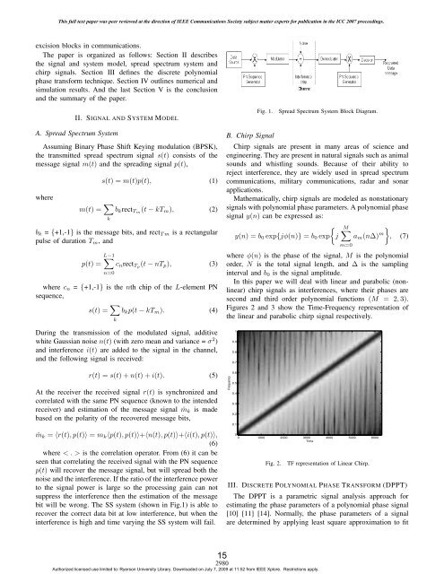
bit will be wrong. The SS system (shown in Fig.1) is able to
recover the correct data bit at low interference, but when the
interference is high and time varying the SS system will fail.
B. Chirp Signal
Fig. 1. Spread Spectrum System Block Diagram.
Chirp signals are present in many areas of science and
engineering. They are present in natural signals such as animal
sounds and whistling sounds. Because of their ability to
reject interference, they are widely used in spread spectrum
communications, military communications, radar and sonar
applications.
Mathematically, chirp signals are modeled as nonstationary
signals with polynomial phase parameters. A polynomial phase
signal y(n) can be expressed as:
M
y(n) =b0 exp{jφ(n)} = b0 exp j am(n∆) m
, (7)
m=0
where φ(n) is the phase of the signal, M is the polynomial
order, N is the total signal length, and ∆ is the sampling
interval and b0 is the signal amplitude.
In this paper we will deal with linear and parabolic (nonlinear)
chirp signals as interferences, where their phases are
second and third order polynomial functions (M = 2, 3).
Figures 2 and 3 show the Time-Frequency representation of
the linear and parabolic chirp signal respectively.
Frequency
1
0.9
0.8
0.7
0.6
0.5
0.4
0.3
0.2
0.1
0
0 1000 2000 3000
Time
4000 5000 6000
Fig. 2. TF representation of Linear Chirp.
III. DISCRETE POLYNOMIAL PHASE TRANSFORM (DPPT)
The DPPT is a parametric signal analysis approach for
estimating the phase parameters of a polynomial phase signal
[10] [11] [14]. Normally, the phase parameters of a signal
are determined by applying least square approximation to fit
15
2980
Authorized licensed use limited to: Ryerson University Library. Downloaded on July 7, 2009 at 11:52 from IEEE Xplore. Restrictions apply.