Signal Analysis Research (SAR) Group - RNet - Ryerson University

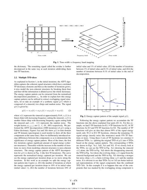
Frequency bands
F4
F3
F2
F1
ME5
s1 s2 ...........................sn
Time−width
ME5 = ME1 + ME2 + ME3 + ME4
SPLIT
the dictionary. The remaining signal called the residue is further
decomposed in the same way at each iteration subdividing them
into TF functions.
2.2. Multiple TFD slices
As explained in Section 1, in the initial iterations, the ATFT algorithm
captures the coherent signal structures which have correlated
TF dictionary elements and then as the number of iterations grows,
it tries model the non-coherent structures by breaking them finer
and finer till the information is diluted across the whole dictionary.
The energy capture pattern can be extracted from the normalized
decomposition parameter an. In order to explain how this energy
capture pattern can be utilized to extract overlapping signal structures,
let us take an example of a synthetic signal y(t) which is
composed of a sinusoid, two chirps and random noise. The signal
y(t) is given by:
y(t) =w1s(t)+w2c1(t)+w3c2(t)+w4r(t) (2)
where s(t) represent the sinusoid at approximately Fs/4, c1(t) is a
linear chirp with increasing frequency cutting the sinusoid, c2(t) is
another linear chirp with decreasing frequency again cutting both
the sinusoid and c1(t). r(t) represents the random noise. The
weight factors w1,2,3,4 are (1, .1, .01, .001) respectively. We performed
the ATFT decomposition (1000 iterations) of y(t) using a
Gabor dictionary. Figures 3(a) and 3(b) show y(t) in time domain
and TF domain (spectrogram is used inorder to show all the three
components at the same time). Here we deliberately introduced energy
differences between the components so as to demonstrate the
significance of energy capture pattern. Most of the times, the first
few iterations capture significant amount of signal energy (coherent
structures). Thereafter with the increase in the number of iterations
we move from modeling coherent structures to non-coherent
structures. The energy capture pattern of the ATFT decomposition
for y(t) is shown in Fig. 2 (the first 50 iterations). The curve
represents the normalized energy captured per iteration. We can
see the energy captured per iteration drops as we move along the
iterations. In this work as an example we split the energy capture
pattern into 4 parts i.e. (E1) the number of iterations at which
the energy captured per iteration drops to 10% of its initial value
(initial value= 1), (E2) the number of iterations between 10% of
Frequency band
ME4
ME3
ME2
ME1
Fig. 1. Time-width vs frequency band mapping
V - 478
81
Time−width
initial value and 1% of initial value, (E3) the number of iterations
between 1% of initial value and 0.1% of initial value, and (E4) the
number of iterations between 0.1% of initial value to the end of
decomposition.
Normalized energy capture curve − log scale
10 0
10 −1
10 −2
10 −3
0.1
0.01
0.001
E1 E2 E3 E4
Energy decomposition pattern( E1, E2, E3 and E4)
10
0 5 10 15 20 25 30 35 40 45 50
−4
Number of iterations
Fig. 2. Energy capture pattern of the sample signal y(t).
Following the energy capture pattern we accumulate the TF
functions into the above explained four parts (E1-4). For this example,
we had 5 TF functions for E1, 9 TF functions for E2, 16 TF
functions for E3 and 970 TF functions for E4. The number of TF
functions will give an idea that almost 99% of the signal energy
needs only 30 (1 to E3) TF fucntions, whereas the remaining 1%
signal energy (mostly noise like strutcures) needs 970 TF functions
or more. Using these 4 sets of TF fucntions we construct 4
different TFDs. i.e. splitting the original TFD of y(t) into 4 TFDs
based on the energy capture pattern. The corresponding 4 TFDs
are shown in Figs. 3(c), 3(d), 3(e) and 3(f). If we closely look at
the TFDs, we can see the TFD in Fig. 3(c) showing the sinusoid
s(t) alone, the TFD in Fig. 3(d) shows the disappearing sinusoid,
the TFD in Fig. 3(e) shows the evolving chirp c1(t) signal from the
sinusoid background and the TFD in Fig. 3(f) showing a stronger
but noisy chirp c1(t), a faint evolving chirp c2(t) and the random
noise. It is obvious to see that TFDs 3(c) to 3(f) are better individual
representations of the signal components than the combined
TFD 3(b). In this example if it so happens that one of the components
that was masked by the overlapping strong component is
Authorized licensed use limited to: Ryerson University Library. Downloaded on July 7, 2009 at 11:11 from IEEE Xplore. Restrictions apply.