3D DISCRETE DISLOCATION DYNAMICS APPLIED TO ... - NUMODIS

Recommendations

Info

20 Description of the simulation method Effective stresses After the internal (σint) and the applied stresses (σapp) are computed, the force on a slip system is defined by the Peach-Koehler equation and a projection along the glide direction g as shown in Eq.2.7. , where l is the unit vector tangent to the dislocation line. τg b = {[(σint + σapp) · b] × l} .g (2.7) It should be noted that σint and σapp are computed at the center of a given segment on the assumption that the stress field variations are small over the segment length. The effective stress τe is then computed by summing all the contributions as τe = τg + τlt − τp. Then, the velocity of the dislocation segment is given by Eq. 2.13. 2.2.2 Computation of displacements The computation of the displacement field of dislocations is very useful not only in analyzing surface deformation induced by dislocations, but also in imposing displacement boundary conditions in a coupling method with a finite element method (Sec. 2.4.2). The displacement solution of any closed curved dislocations can be found from the Burgers formula in the frame of elastic isotropy. The Burgers equation is given in terms of line and area integrals as shown in Eq. 2.8 in a vector form. u(r) = − b 1 b × dl Ω − 4π 4π C ′ R + 1 8π(1 − ν) ∇ (b × R) dl C ′ R b is the Burgers vector and ν is the Poisson ratio. Ω is the solid angle through which the positive side of a loop is seen and is defined as follows. RdA Ω = − A R3 The parameters for the computation Eq. 2.8 and Eq. 2.9 are shown for the configuration of a closed loop in Fig. 2.8. An analytical solution of the displacement fields can be obtained using Eq. 2.8 for the case of simple dislocation loops 7 . The solutions of complex dislocation loops are generally difficult to be resolved analytically. The general way of computing a displacement field of an arbitrary dislocation loop is to decompose the loop into triangular loops as illustrated in Fig. 2.8. The methodology to construct a displacement field from triangular loops was first presented by Hirth and Lothe (see 7 Khraishi et al. ([Khraishi et al. 00b]) have found a closed-form analytical solution of a circular dislocation loop. (2.8) (2.9)
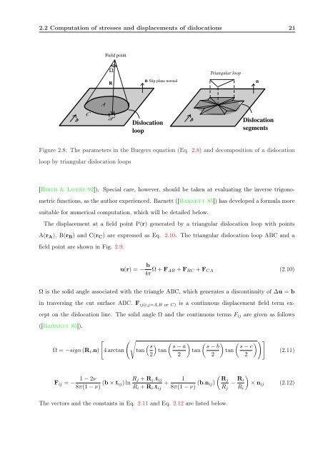
2.2 Computation of stresses and displacements of dislocations 21 b C A Field point Ω R dl’ n Slip plane normal Dislocation loop b Triangular loop n Dislocation segments Figure 2.8: The parameters in the Burgers equation (Eq. 2.8) and decomposition of a dislocation loop by triangular dislocation loops [Hirth & Lothe 92]). Special care, however, should be taken at evaluating the inverse trigono- metric functions, as the author experienced. Barnett ([Barnett 85]) has developed a formula more suitable for numerical computation, which will be detailed below. The displacement at a field point P(r) generated by a triangular dislocation loop with points A(rA), B(rB) and C(rC) are expressed as Eq. 2.10. The triangular dislocation loop ABC and a field point are shown in Fig. 2.9. u(r) = − b 4π Ω + FAB + FBC + FCA (2.10) Ω is the solid angle associated with the triangle ABC, which generates a discontinuity of ∆u = b in traversing the cut surface ABC. F ij(i,j=A,B or C) is a continuous displacement field term ex- cept on the dislocation line. The solid angle Ω and the continuous terms Fij are given as follows ([Barnett 85]). s s − a s − b s − c Ω = −sign (Ri.n) 4 arctan tan tan tan tan 2 2 2 2 Fij = − 1 − 2ν 8π(1 − ν) (b × tij) ln Rj + Rj.tij Ri + Ri.tij + 1 8π(1 − ν) (b.nij) Rj Rj The vectors and the constants in Eq. 2.11 and Eq. 2.12 are listed below. − Ri × nij Ri (2.11) (2.12)
Page 1 and 2: INSTITUT NATIONAL POLYTECHNIQUE DE
Page 3: Acknowledgements First of all, I ex
Page 6 and 7: Résumé La dynamique des dislocati
Page 8 and 9: viii CONTENTS 2.3.5 Plastic strain
Page 11 and 12: Chapter 1 Introduction 1.1 Computat
Page 13 and 14: 1.2 Dislocation dynamics 3 (a) Weak
Page 15 and 16: 1.3 Scope of Thesis 5 Recently the
Page 17: 1.3 Scope of Thesis 7 coupling meth
Page 20 and 21: 10 Description of the simulation me
Page 61 and 62: Chapter 3 Parallelization of the Di
Page 63 and 64: 3.1 An introduction to Supercomputi
Page 71 and 72: 3.2 Towards a parallel DDD code 61
Page 77 and 78: 3.3 Parallelization of the serial D
Page 79 and 80: 3.3 Parallelization of the serial D
Page 81 and 82:
3.3 Parallelization of the serial D
Page 83 and 84:
Page 85 and 86:
Page 87 and 88:
Page 89 and 90:
Page 91 and 92:
3.4 Performance improvment 81 Speed
Page 93 and 94:
Page 95 and 96:
Page 97 and 98:
3.4 Performance improvment 87 Y Z I
Page 99 and 100:
3.5 Application to Stage I-II trans
Page 101 and 102:
Page 103 and 104:
Page 105 and 106:
Chapter 4 Dislocation-precipitate i
Page 107 and 108:
4.1 Image stresses due to a 3D part
Page 109 and 110:
Page 111 and 112:
Page 113 and 114:
Page 115 and 116:
4.2 A simple case of dislocation-pa
Page 117 and 118:
Page 119 and 120:
Page 121 and 122:
Page 123 and 124:
Page 125 and 126:
Page 127 and 128:
4.3 Fatigue simulations of material
Page 129 and 130:
Page 131 and 132:
Page 133 and 134:
Page 135 and 136:
Page 137 and 138:
Page 139 and 140:
Page 141 and 142:
Page 143 and 144:
Page 145 and 146:
Page 147 and 148:
Page 149 and 150:
Page 151 and 152:
Page 153 and 154:
Page 155 and 156:
Page 157 and 158:
Page 159 and 160:
Chapter 5 Conclusions and perspecti
Page 161 and 162:
namics codes into a parallel versio
Page 163 and 164:
Bibliography [Abraham 97] Abraham F
Page 165 and 166:
BIBLIOGRAPHY 155 [Devincre & Robert
Page 167 and 168:
BIBLIOGRAPHY 157 [Khraishi et al. 0
Page 169 and 170:
BIBLIOGRAPHY 159 [Risbet et al. 03]
show all

3D DISCRETE DISLOCATION DYNAMICS APPLIED TO ... - NUMODIS

Create successful ePaper yourself

Delete template?

Save as template?