3D DISCRETE DISLOCATION DYNAMICS APPLIED TO ... - NUMODIS

30 Description of the simulation method
0 1 ... ... L-2 L-1
L-1
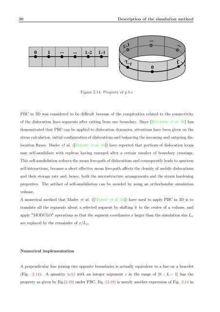
Figure 2.14: Property of p.b.c
PBC in 3D was considered to be difficult because of the complexities related to the connectivity
of the dislocation lines segments after exiting from one boundary. Since [Bulatov et al. 01] has
demonstrated that PBC can be applied to dislocation dynamics, attentions have been given on the
stress calculation, initial configuration of dislocations and balancing the incoming and outgoing dis-
location fluxes. Madec et al. ([Madec et al. 04]) have reported that portions of dislocation loops
may self-annihilate with replicas having emerged after a certain number of boundary crossings.
This self-annihilation reduces the mean free-path of dislocations and consequently leads to spurious
self-interactions, because a short effective mean free-path affects the density of mobile dislocations
and their storage rate and, hence, both the microstructure arrangements and the strain hardening
properties. The artifact of self-annihilation can be avoided by using an orthorhombic simulation
volume.
A numerical method that Madec et al. ([Madec et al. 04]) have used to apply PBC in 3D is to
translate all the segments about a selected segment by shifting it to the center of a volume, and
apply "MODULO" operations so that the segment coordinates x larger than the simulation size Lx
are replaced by the remainder of x/Lx.
Numerical implementation
A perpendicular line joining two opposite boundaries is actually equivalent to a line on a bracelet
(Fig. 2.14). A quantity ic(i) with an integer argument i in the range of [0 : L − 1] has the
property as given by Eq.(2.19) under PBC. Eq. (2.19) is merely another expression of Fig. 2.14 in
L-2
...
0
...
1