Engineering geology of British rocks and soils Mudstones of the ...

Table 6.3 Stratigraphical subdivisions for Areas 1, 3 and 8.
AREA 1 LKM Lower Keuper Marl
MKM Middle Keuper Marl
LKSB Lower Keuper Saliferous Beds
UKSB Upper Keuper Saliferous Beds
AREA 3 TwM Twyning Mudstone Formation
Eld Eldersfield Mudstone Formation
AREA 8 Cbp Cropwell Bishop Formation
Edw Edwalton Formation
Gun Gunthorpe Formation
HlyHollygate Sandstone
Rdc Radcliffe Formation
Snt Sneinton Formation
caused by depth, and other, related factors, and to characterise
engineering behaviour at deep and shallow levels
(Figures 7.2 to 7.18). Weathering may be related in a general
sense to depth below ground level, but this is not a simple
relationship of decreasing weathering with increasing depth
in the case of the Mercia Mudstone. Moisture content,
density, permeability, and strength may also relate to depth.
A large proportion of the database was assembled from
highway site investigations. Many of these have been carried
out on embankments or in cuttings, for example where
existing roads are to be widened. This means that ground
levels reported in the site investigation are not necessarily
original natural ground levels. Plots of parameters with
depth should therefore be treated with some caution as they
contain random errors, and only give a general trend. Depth
relationships shown here should not be used in design calculations.
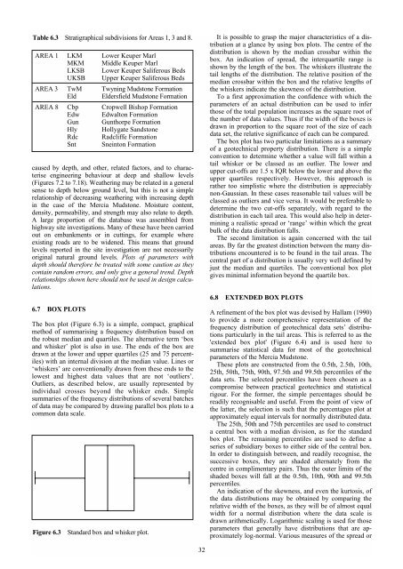
6.7 BOX PLOTS
The box plot (Figure 6.3) is a simple, compact, graphical
method of summarising a frequency distribution based on
the robust median and quartiles. The alternative term ‘box
and whisker’ plot is also in use. The ends of the box are
drawn at the lower and upper quartiles (25 and 75 percentiles)
with an internal division at the median value. Lines or
‘whiskers’ are conventionally drawn from these ends to the
lowest and highest data values that are not ‘outliers’.
Outliers, as described below, are usually represented by
individual crosses beyond the whisker ends. Simple
summaries of the frequency distributions of several batches
of data may be compared by drawing parallel box plots to a
common data scale.
Figure 6.3 Standard box and whisker plot.
32
It is possible to grasp the major characteristics of a distribution
at a glance by using box plots. The centre of the
distribution is shown by the median crossbar within the
box. An indication of spread, the interquartile range is
shown by the length of the box. The whiskers illustrate the
tail lengths of the distribution. The relative position of the
median crossbar within the box and the relative lengths of
the whiskers indicate the skewness of the distribution.
To a first approximation the confidence with which the
parameters of an actual distribution can be used to infer
those of the total population increases as the square root of
the number of data values. Thus if the width of the boxes is
drawn in proportion to the square root of the size of each
data set, the relative significance of each can be compared.
The box plot has two particular limitations as a summary
of a geotechnical property distribution. There is a simple
convention to determine whether a value will fall within a
tail whisker or be classed as an outlier. The lower and
upper cut-offs are 1.5 x IQR below the lower and above the
upper quartiles respectively. However, this approach is
rather too simplistic where the distribution is appreciably
non-Gaussian. In these cases reasonable tail values will be
classed as outliers and vice versa. It would be preferable to
determine the two cut-offs separately, with regard to the
distribution in each tail area. This would also help in determining
a realistic spread or ‘range’ within which the great
bulk of the data distribution falls.
The second limitation is again concerned with the tail
areas. By far the greatest distinction between the many distributions
encountered is to be found in the tail areas. The
central part of a distribution is usually very well defined by
just the median and quartiles. The conventional box plot
gives minimal information beyond the quartile box.
6.8 EXTENDED BOX PLOTS
A refinement of the box plot was devised by Hallam (1990)
to provide a more comprehensive representation of the
frequency distribution of geotechnical data sets’ distributions
particularly in the tail areas. This is referred to as the
'extended box plot' (Figure 6.4) and is used here to
summarise statistical data for most of the geotechnical
parameters of the Mercia Mudstone.
These plots are constructed from the 0.5th, 2.5th, 10th,
25th, 50th, 75th, 90th, 97.5th and 99.5th percentiles of the
data sets. The selected percentiles have been chosen as a
compromise between practical geotechnics and statistical
rigour. For the former, the simple percentages should be
readily recognisable and useful. From the point of view of
the latter, the selection is such that the percentages plot at
approximately equal intervals for normally distributed data.
The 25th, 50th and 75th percentiles are used to construct
a central box with a median division, as for the standard
box plot. The remaining percentiles are used to define a
series of subsidiary boxes to either side of the central box.
In order to distinguish between, and readily recognise, the
successive boxes, they are shaded alternately from the
centre in complimentary pairs. Thus the outer limits of the
shaded boxes will fall at the 0.5th, 10th, 90th and 99.5th
percentiles.
An indication of the skewness, and even the kurtosis, of
the data distributions may be obtained by comparing the
relative width of the boxes, as they will be of almost equal
width for a normal distribution where the data scale is
drawn arithmetically. Logarithmic scaling is used for those
parameters that generally have distributions that are approximately
log-normal. Various measures of the spread or