Extended Abstract

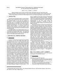
8.2 SCIPUFF CAPABILITIES AND APPLICATION IN HAZARD ASSESSMENT
1. INTRODUCTION
R. Ian Sykes *
Sage Management Enterprise, Princeton NJ
SCIPUFF, Second-order Closure Integrated PUFF,
is an atmospheric dispersion model using the Gaussian
puff methodology to provide a three-dimensional, timedependent
Lagrangian solution to the turbulent diffusion
equations. Originally developed for the prediction of
power plant plume impacts under the sponsorship of
EPRI (Electric Power Research Institute), SCIPUFF has
been extensively enhanced under DoD (Department of
Defense) funding, and now describes a wide range of
phenomena beyond buoyant plume rise and turbulent
diffusion.
2. LAGRANGIAN PUFF TECHNIQUE
The time-dependent concentration field is
represented as a collection of overlapping Gaussian
puffs, where the Gaussian shape is described by a total
mass, a centroid location, and measure of the spatial
spread. The puffs are transported as Lagrangian
elements, providing a grid-independent description of
diffusion in inhomogeneous, time-dependent
meteorology. The puff methodology can also describe
multiple releases of multiple materials simultaneously.
with arbitrary time-dependent and spatial
characteristics.
In SCIPUFF, the spatial Gaussian spread is
represented in a general tensor form using the full
second-moments of the concentration field, including
the off-diagonal moments, so that shear distortion can
be accurately described. The transport equation for the
spatial moments is based on second-order turbulence
closure theory, which directly relates the diffusion rates
to the measurable velocity statistics. This provides a
methodology that is valid over all scales, and provides a
rational basis for the treatment of time averaging effects
based on the assumed shape of the velocity fluctuation
spectrum (Sykes and Gabruk, 1997). The closure
model gives an idealized prediction that is consistent
with the analytical results of Taylor (1921) for absolute
dispersion, and Richardson (1926) for relative diffusion.
The evolution equation for the spatial spread
moments is written as
dσ ∂u ∂u
x′ i u′ j c′ x′ j u′ i c′
= σ + σ + +
dt x x Q Q
ij j i
ik
∂ k
jk
∂ k
where σ ij is the moment tensor, Q is the material mass
in the puff, and the angle brackets indicate an integral
over the puff. The first two terms represent shear
distortion, and the last two are the spatial moments of
*Corresponding author address: R. Ian Sykes, Sage
Management, 15 Roszel Road, Suite 102, Princeton NJ
08540; e-mail: ian.sykes@sage-mgt.net.
the turbulent concentration flux, which is responsible for
diffusion. The flux moment equations are derived from
the closure model as
d q
x′ i u′ j c′ = Qu′ i u′ j − A x′ i u′ j c′
dt
Λ
where
= ′ ′ is the turbulent velocity scale, Λ is the
2
q ui ui
turbulent length scale, and A is a closure constant with a
value of 0.75.
3. SCIPUFF MODEL CAPABILITIES
The closure model provides a natural framework for
predicting the concentration fluctuation variance, since
this is a second-order quantity. The concentration
fluctuations are driven by the turbulent velocity
fluctuations and represent a statistical uncertainty in any
measured concentration value. Using an assumed
probability distribution shape for the fluctuations, based
on the predicted mean and variance, we can provide a
quantitative probability prediction for the concentration.
Since the fluctuation variance is a nonlinear
quantity, we need to extend the simple puff model,
where each puff moves and evolves independently, by
calculating the overlap contributions from puffs that are
closely located. The variance is predominantly
controlled by the turbulent dissipation, and modeling this
term requires an evolution for an internal fluctuation
length scale. Results for the fluctuation intensity
compared with the laboratory experiments of Fackrell
and Robins (1982) are shown in Figure 1.
σ c
c
6
4
2
d s = 3mm
9mm
15mm
25mm
35mm
0
0 2 4 6 8 10
x H
Fig. 1. SCIPUFF prediction of centerline fluctuation
intensity in an elevated plume for different source
sizes. Symbols are data from Fackrell and
Robins (1982), model predictions are solid lines.
The implementation of the puff overlap calculations
in SCIPUFF enables other nonlinear processes to be
described. Specifically, some of the major dynamics
processes can be represented by providing evolution

Z (m)
equations for integrated momentum and buoyancy for
each puff, and assuming simple spatial shape functions
for the associated velocity fields (Sykes et al. 1999).
The equations for the integrated moments are based on
the Navier-Stokes conservation equations, and give a
reasonable representation of buoyant jets and dense
gas slumping effects. Figure 2 shows an idealized
calculation of two buoyant plumes in a vertical shear
environment.
Fig. 2. SCIPUFF prediction of buoyant plumes in a
simplified wind shear.
In addition to dynamics, SCIPUFF can also
represent evaporating droplets and the associated
thermodynamics effects. Figure 3 shows a flashing
chlorine jet with initial upward momentum, but the
cooling associated with the evaporation generates a
cold chlorine vapor cloud which then slumps on the
ground.
and dense effects
Fig. 3. SCIPUFF prediction of flashing chlorine jet.
As a final example, SCIPUFF has also been
enhanced to describe nonlinear gas phase chemical
reactions. The puff overlap calculations are used to
estimate the total Gaussian-weighted concentration of
each chemical species for each puff. The chemical
reaction mechanism is used to determine the effective
change in concentrations over a timestep, and the puff
species masses are adjusted in proportion to their
contribution to the concentration. Figure 4 shows the
SCIPUF prediction of ozone depletion and subsequent
formation downwind of a NOx source, using the Carbon
Bond Mechanism.
4. SCIPUFF MODEL NUMERICAL FEATURES
A key feature of SCIPUFF is the splitting/merging
algorithms which improve the representation of
inhomogeneous meteorology. The shear and diffusion
terms in the moment equations are based on local
z
U
Fig. 4. SCIPUFF prediction of ozone downwind of a NOx
source, shown as the small triangle in the lower
half of the plot.
values of wind, wind shear and turbulence, and cannot
accurately represent more complex fields. Puffs are
split, conserving all the moments, when they reach a
size comparable with the scale of the meteorological
grid; similarly, puffs are merged when they grow large
enough to overlap their neighbors sufficiently.
SCIPUFF uses adaptive timesteps and adaptive
spatial grids to represent concentration, dosage, and
deposition fields. These techniques are well suited to
Lagrangian models, where very large ranges of scales
need to be represented. Near the source, puffs may
have scales of a few meters or less, but the model is
required to calculate effects at ranges up to 1000’s of
kilometers.
SCIPUFF has been evaluated using a wide range
of field experiments, ranging from the short range
CONFLUX experiments with downwind range of several
meters up to the ANATEX and ETEX continental scale
experiments.
5. ROLE IN HAZARD MODELING SYSTEMS
SCIPUFF is the atmospheric dispersion modeling
component of two US Department of Defense hazard
prediction systems. The systems are HPAC, Hazard
Prediction and Assessment Capability and JEM, the
Joint effects Model, HPAC is developed by the Defense
Threat Reduction Agency and JEM is a DoD Program of
Record under the Joint Program Executive Office for
Chemical and Biological Defense (JPEO CBD). The
two systems are described at:
http://www.dtra.mil/rd/programs/acec/hpac.cfm, and
https://jacks.jpeocbd.army.mil/jacks/Public/FactSheetPr
ovider.aspx?productId=335
Both of these systems comprise much more than
the SCIPUFF dispersion model. They also include:

• source term models for various incidents
• weapon deployments
• facilities attacks or explosive events
• human effects models
• chemical/biological effects
• nuclear radiation
• global population database
• casualty estimation
• urban dispersion nested models
• building database
• meteorological data servers
• forecast and observations
• global terrain database
These capabilities are essential for predicting
hazard effects. The availability of meteorological data is
crucial, and must be provided in a timely manner. Also,
the prediction of human effects is an important aspect,
for consequence assessment. The broad range of
capabilities in SCIPUFF has been developed to provide
the atmospheric dispersion calculation, linking the
source term models with the human effects models. A
sample output display from HPAC is shown in Figure 5.
5. REFERENCES
Fackrell, J.E. & A.G. Robins (1982), Concentration
fluctuations and fluxes in plumes from a point source
in a turbulent boundary layer, J. Fluid Mech.,117,1-26.
Richardson, L. F. (1926), "Atmospheric Diffusion shown
on a DistanceNeighbour Graph", Proc. Roy. Soc.
Lond. A, 110, 709-737
Sykes, R. I. and R. S. Gabruk (1997), "A second-order
closure model for the effect of averaging time on
turbulent plume dispersion", J. Appl. Met, 36, 165-184
Sykes, R. I., C. P. Cerasoli and D. S. Henn (1999), "The
representation of dynamic flow effects in a Lagrangian
puff dispersion model", J. Haz. Mat., A:64, 223-247
Taylor, G. I. (1921), "Diffusion by continuous
movements", Proc. Lond. Math. Soc. (Ser. 2), 20,
196-211
Figure 5. Sample HPAC output display illustrating the building effects submodel, building database, and
human effects output with casualty estimation