Extended Abstract - AMS supported meetings

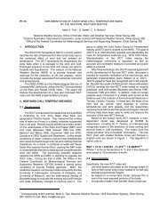
This paper covers the content of papers 7B.1 & 7B.2 (File size for the 2 papers is 3,067 KB) 

Short-Term Forecasting of Severe Convective Storms Using Quantitative Multi-Spectral, 

Satellite Imagery: Results of the Early Alert Project 

William L. Woodley 1 , Daniel Rosenfeld 2 , Guy Kelman 2 and Joseph H. Golden 3 

1 Woodley Weather Consultants, 2 Hebrew University of Jerusalem, 3 Cooperative Institute 

for Research in the Environmental Sciences 

1.0 BACKGROUND 

A team of research scientists has been 

working under the auspices of Woodley 

Weather Consultants (WWC) with the 

support of NOAA’s Small Business 

Innovative Research Program (SBIR) to 

develop and test a method to provide 

satellite, microphysically-based, ―Early 

Alerts‖ (EA) of severe convective storms 

(tornadoes, hail and strong, straight-line, 

downburst winds). The method objective is 

to predict when and where a severe weather 

is most likely to occur one to two hours 

prior to the actual event, potentially saving 

lives and property. This report documents 

the development and testing of the 

methodology, including its scientific basis 

and the underlying conceptual model, the 

initial work with AVHRR multi-spectral 

data from polar-orbiting satellites, the 

adaptation of the method to accept real-time 

GOES multi-spectral data, and the real-time 

testing of the method at the Storm Prediction 

Center in Norman, Oklahoma. 

As discussed in Section 2.0 herein, the 

new method is based on a conceptual model 

that facilitates the inference of the 

------------------------------------------------------ 

Corresponding author address: William L. 

Woodley, Woodley Weather Consultants, 11 

White Fir Court, Littleton, Colorado 80127; 

e-mail:williamlwoodley@cs.com 

vigor of severe convective storms, 

producing tornadoes and large hail, by using 

satellite-retrieved vertical profiles of cloud 

top temperature (T) and particle effective 

radius (r e ). The driving force of these severe 

weather phenomena is the high updraft 

speed, which can sustain the growth of large 

hailstones and provide the upward motion 

that is necessary to evacuate the violently 

converging air of a tornado. Stronger 

updrafts are revealed by the delayed growth 

of r e to greater heights and lower T, because 

there is less time for the cloud and rain 

drops to grow by coalescence. The strong 

updrafts also delay the development of a 

mixed phase cloud and its eventual 

glaciation to colder temperatures. In addition 

to the presentation of the conceptual model 

and the derivation of the method, this 

section documents the initial testing of the 

concepts using multi-spectral AVHRR data 

from polar-orbiting satellites. 

Even though this work validated the 

conceptual model, it had minimal practical 

forecast value because it was based on 

imagery that was available only once or 

twice per day. Greater image frequency was 

needed. Section 3 gives the results of initial 

testing under SBIR-1 of the concepts and 

method using GOES multi-spectral imagery 

that was available at 30 min intervals. The 

concepts and methods proved robust to this 

testing, and the question arose whether a 

1

eal-time version of the method could be 

developed to improve severe storm watches 

and warnings. Doing this was the focus of 

SBIR-2. As discussed in Section 5.0, this 

entailed the development of a real-time 

version of the method that was tested at the 

Storm Prediction Center (SPC) during the 

spring of 2008. 

2.0 INITIAL CONCEPTUAL TESTING 

2.1 Scientific Basis 

This study builds on the paper by 

Rosenfeld et al. (2007) that provides the 

scientific basis and background for the new 

conceptual model to be discussed here that 

facilitates the detection of the vigor of 

convective storms by remote sensing from 

satellites, based on the retrieved vertical 

profiles of cloud-particle effective radius 

and thermodynamic phase. Severe 

convective storms are defined by the US 

National Weather Service as having wind 

gusts > 58 mph, hail > 3/4 inch in diameter, 

or producing tornadoes. A major driving 

force of all these severe weather phenomena 

is the high updraft speeds, which can sustain 

the growth of large hailstones, provide the 

upward motion that is necessary for 

evacuating vertically the violently 

converging air of a tornado, or 

complemented strong downward motion, 

which results in downbursts and intense gust 

fronts. Wind shear provides additional 

energy for sustaining the dynamics of 

tornadic super-cell storms and squall lines 

that can re-circulate large hailstones and 

produce damaging winds. The respective 

roles of convective potential available 

energy (CAPE) and the 0-6 km vertical wind 

shear have been the main predictors for 

severe convective storms (Rasmussen and 

Blanchard, 1998; Hamill and Church, 2000; 

Brooks et al., 2003). The existence of wind 

shear and low-level storm relative helicity 

(rotation of the wind vector) were found to 

be associated with strong (at least F2) 

tornadoes (Dupilka and Reuter, 2006a and 

2006b). However, even with small helicity, 

a steep low level lapse rate and large CAPE 

can induce strong tornadoes due to the large 

acceleration of the updrafts already at low 

levels (Davis, 2006). This underlines the 

importance of the updraft velocities in 

generating the severe convective storms, and 

the challenges involved in their forecasting 

based on sounding data alone. 

The conceptual model of a satelliteobserved 

severe storm microphysical 

signature that is addressed in this paper is 

based on the satellite-retrieved 

microphysical signature of the updraft 

velocity of the developing convective 

elements that have the potential to become 

severe convective storms, or already 

constitute the feeders of such storms. The 

severe storm microphysical signature, as 

manifested by the vertical profile of cloudparticle 

effective radius, is caused by the 

greater updrafts delaying to greater heights 

the conversion of cloud drops to 

hydrometeors and the glaciation of the 

cloud. The greater wind shear tilts the 

convective towers of the pre-storm and 

feeder clouds and often deflects the strongly 

diverging cloud tops from obscuring the 

feeders. This allows the satellite a better 

view of the microphysical response of the 

clouds to the strong updrafts. This satellite 

severe storm signature appears to primarily 

reflect the updraft speed of the growing 

clouds, which is normally associated with 

the CAPE. But wind shear is as important as 

CAPE for the occurrence of severe 

convective storms, in addition to helicity 

that is an important ingredient in intense 

tornadoes. It is suggested that the 

effectiveness of the satellite retrieved severe 

storm signature and inferred updraft speed 

may not only depend on the magnitude of 

2

the CAPE, but also on the wind shear, and 

perhaps also on the helicity. This can occur 

when some of the horizontal momentum is 

converted to vertical momentum in a highly 

sheared environment when strong inflows 

are diverted upward, as often happens in 

such storms. While this study focuses on 

exploring a new concept of satellite 

application, eventually a combined satellite 

with a sounding algorithm is expected to 

provide the best skill. 

2.1.1 Direct observations of cloud top 

dynamics for inferences of updraft 

velocities and storm severity 

Updraft speeds are the most direct 

measure of the vigor of a convective storm. 

The updraft speeds of growing convective 

clouds can be seen in the rise rate of the 

cloud tops, or measured from satellites as 

the cooling rate of the tops of these clouds. 

A typical peak value of updrafts of severe 

storms exceeds 30 ms -1 (e.g., Davies-Jones, 

1974). Such strong updrafts are too fast to 

be detected by a sequence of geostationary 

satellite images, because even during a 5 

minute rapid scan an air parcel moving at 30 

ms -1 covers 9 km if continued throughout 

that time (super-rapid scans of up to one per 

30 – 60 s can be done, but only for a small 

area and not on a routine operational basis). 

But such strong updrafts occur mainly at the 

supercooled levels, where the added height 

of 9 km will bring the cloud top to the 

tropopause in less than 5 minutes. In 

addition, the cloud segments in which such 

strong updrafts occur are typically smaller 

than the resolution of thermal channels of 

present day geostationary satellites (5 to 8 

km at mid latitudes). This demonstrates that 

both the spatial and temporal resolutions of 

the current geostationary satellites are too 

coarse to provide direct measurements of the 

updraft velocities in severe convective 

clouds. The overshooting depth of cloud 

tops above the tropopause can serve as a 

good measure of the vigor of the storms, but 

unfortunately the brightness temperatures of 

overshooting cloud tops do not reflect their 

heights due to the generally isothermal 

nature of the penetrated lower stratosphere. 

Overshooting severe convective storms 

often develop a V shape feature downwind 

of their tallest point, which appears as a 

diverging plume above the anvil top 

(Heymsfield et al., 1983; McAnn, 1983). 

The plume typically is highly reflective at 

3.7 µm, which means that it is composed of 

very small ice particles (Levizzani and 

Setvák, 1996, Setvák et al., 2003). A warm 

spot at the peak of the V is also a common 

feature, which is likely caused by the 

descending stratospheric air downwind of 

the overshooting cloud top. Therefore, the 

V-shape feature is a dynamic manifestation 

of overshooting tops into the lower 

stratosphere when strong storm-relative 

winds occur there. The observation of a V- 

shape feature reveals the existence of the 

combination of intense updrafts and wind 

shear. Adler et al. (1983) showed that most 

of the storms that they examined in the US 

Midwest (75%) with the V-shape had severe 

weather, but many severe storms (45%) did 

not have this feature. Adler et al. (1983) 

showed also that the rate of expansion of 

storm anvils was statistically related 

positively to the occurrences of hail and 

tornadoes. All this suggests that satellite 

inferred updraft velocities and wind shear 

are good indicators for severe storms. While 

wind shear is generally easily inferred from 

synoptic weather analyses and predictions, 

the challenge is the inference of the updraft 

intensities from the satellite data. The 

manifestation of updraft velocities in the 

cloud microstructure and thermodynamic 

phase, which can be detected by satellites, is 

the subject of the next section. 

3

2.1.2 Anvil tops with small particles at 

-40°C reflecting homogeneouslyglaciating 

clouds 

Small ice particles in anvils or cirrus 

clouds typically form as a result of either 

vapor deposition on ice nuclei, or by 

homogeneous ice nucleation of cloud drops 

which occurs at temperatures colder than - 

38°C. In deep convective clouds 

heterogeneous ice nucleation typically 

glaciates the cloud water before reaching the 

-38°C threshold. Clouds that glaciate mostly 

by heterogeneous nucleation (e.g. by ice 

multiplication, ice-water collisions, ice 

nuclei and vapor deposition) are defined 

here as glaciating heterogeneously. Clouds 

in which most of their water freezes by 

homogeneous nucleation are defined here as 

undergoing homogeneous glaciation. Only a 

small fraction of the cloud drops freezes by 

interaction with ice nuclei, because the 

concentrations of ice nuclei are almost 

always smaller by more than four orders of 

magnitude than the drop concentrations (ice 

nuclei of ~0.01 cm -3 whereas drop 

concentrations are typically > 100 cm -3 ) 

before depletion by evaporation, 

precipitation or glaciation. Therefore, most 

drops in a heterogeneously glaciating cloud 

accrete on pre-existing ice particles, or 

evaporate for later deposition on the existing 

cloud ice particles. This mechanism 

produces a glaciated cloud with ice particles 

that are much fewer and larger than the 

drops that produced them. In fact, 

heterogeneous glaciation of convective 

clouds is a major precipitation-forming 

mechanism. 

Heterogeneously glaciating clouds with 

intense updrafts (>15 ms -1 ) may produce 

large supersaturations that, in the case of a 

renewed supply of CCN from the ambient 

air aloft, can nucleate new cloud drops not 

far below the -38°C isotherm, which then 

freeze homogeneously at that level (Fridlind 

et al., 2004; Heymsfield et al., 2005). In 

such cases the cloud liquid water content 

(LWC) is very small, not exceeding about 

0.2 g m -3 . This mechanism of homogeneous 

ice nucleation occurs, of course, also at 

temperatures below -38°C, and is a major 

process responsible for the formation of 

small ice particles in high-level strong 

updrafts of deep convective clouds, which 

are typical of the tropics (Jensen and 

Ackerman, 2006). 

Only when much of the condensed cloud 

water reaches the -38°C isotherm before 

being consumed by other processes can the 

cloud be defined as undergoing 

homogeneous glaciation. The first in situ 

aircraft observations of such clouds were 

made recently, where cloud filaments with 

LWC reaching half (Rosenfeld and 

Woodley, 2000) to full (Rosenfeld et al., 

2006b) adiabatic values were measured in 

west Texas and in the lee of the Andes in 

Argentina, respectively. This required 

updraft velocities exceeding 40 ms -1 in the 

case of the clouds in Argentina, which 

produced large hail. The aircraft 

measurements of the cloud particle size in 

these two studies revealed similar cloud 

particle sizes just below and above the level 

where homogeneous glaciation occurred. 

This means that the homogeneously 

glaciating filaments in these clouds were 

feeding the anvils with frozen cloud drops, 

which are distinctly smaller than the ice 

particles that rise into the anvils within a 

heterogeneously glaciating cloud. 

In summary, there are three types of 

anvil compositions, caused by three 

glaciation mechanisms of the convective 

elements: (1) Large ice particles formed by 

heterogeneous glaciation; (2) homogeneous 

glaciation of LWC that was generated at low 

levels in the cloud, and, (3) homogeneous 

glaciation of newly nucleated cloud drops 

near or above the -38°C isotherm level. This 

4

third mechanism occurs mostly in 

cirrocumulus or in high wave clouds, as 

shown in Figure 7a in Rosenfeld and 

Woodley (2003). The manifestations of the 

first two mechanisms in the composition of 

anvils are evident in the satellite analysis of 

cloud top temperature (T) versus cloud top 

particle effective radius (r e ) shown in Figure 

1. In this red-green-blue composite brighter 

visible reflectance is redder, smaller cloud 

top particles look greener, and warmer 

thermal brightness temperature is bluer. This 

analysis methodology (Rosenfeld and 

Lensky, 1998) is reviewed in Section 2.2 of 

this paper. The large ice particles formed by 

heterogeneous glaciation appear red in 

Figure 1 and occur at cloud tops warmer 

than the homogeneous glaciation 

temperature of -38°C. The yellow cloud tops 

in Figure 1 are colder than -38°C and are 

composed of small ice particles that 

probably formed by homogeneous 

glaciation. The homogeneously glaciated 

cloud water appeared to have ascended with 

the strongest updrafts in these clouds and 

hence formed the tops of the coldest clouds. 

The homogeneous freezing of LWC 

generated at low levels in convective clouds 

is of particular interest here, because it is 

indicative of updrafts that are sufficiently 

strong such that heterogeneous ice 

nucleation would not have time to deplete 

much of the cloud water before reaching the 

homogeneous glaciation level. As such, the 

satellite signature in the form of enhanced 

3.7-µm reflectance can be used as an 

indicator of the occurrence of strong 

updrafts, which in turn are conducive to the 

occurrence of severe convective storms. 

This realization motivated Lindsey et al. 

(2006) to look for anvils with high 

Geostationary Operational Environmental 

Satellite (GOES) 3.9-µm reflectance as 

indicators of intense updrafts. They showed 

that cloud tops with 3.9-µm reflectance > 

5% occurred for

the T-r e lines for the clouds in the marked 

rectangle. The different colored lines 

represent different T-r e percentiles every 5% 

from 5% (left most line) to 100% (right most 

line), where the bright green is the median. 

The white line on the left side of the inset is 

the relative frequency of the cloudy pixels. 

The vertical lines show the vertical extent of 

the microphysical zones: yellow for the 

diffusional growth; green for the 

coalescence zone (does not occur in this 

case); pink for the mixed phase and red for 

the glaciated zone. The glaciated cloud 

elements that do not exceed the -38°C 

isotherm appear red and have very large r e 

that is typical of ice particles that form by 

heterogeneous freezing in a mixed phase 

cloud, whereas the colder parts of the anvil 

are colored orange and are composed of 

small particles, which must have formed by 

homogeneous freezing of the cloud drops in 

the relatively intense updraft that was 

necessary to form the anvil portions above 

the -38°C isotherm. 

The concept of "residence time" fails for 

clouds that have warm bases, because even 

with CAPE that is conducive to severe 

storms heterogeneous freezing is reached 

most of the time. This is manifested by the 

fact that clouds with residence times less 

than 100 s and hence with 3.9-µm 

reflectivities greater than 5%, were almost 

exclusively west of about 100 o W, where 

cloud base heights become much cooler and 

higher (Lindsey, personal communications 

pertaining to Figure 7 of his 2006 paper). 

Aerosols play a major role in the 

determination of the vertical profiles of 

cloud microstructure and glaciation. Khain 

et al. (2001) simulated with an explicit 

microphysical processes model the detailed 

microstructure of a cloud that Rosenfeld and 

Woodley (2000) documented, including the 

homogeneous glaciation of the cloud drops 

that had nucleated near cloud base at a 

temperature of about 9°C. When changing in 

the simulation from high to low 

concentrations of CCN, the cloud drop 

number concentration was reduced from 

1000 to 250 cm -3 . Coalescence quickly 

increased the cloud drop size with height 

and produced hydrometeors that froze 

readily and scavenged almost all the cloud 

water at -23°C, well below the 

homogeneous glaciation level. This is 

consistent with the findings of Stith et al. 

(2004), who examined the microphysical 

structure of pristine tropical convective 

clouds in the Amazon and at Kwajalein, 

Marshall Islands. They found that the 

updrafts glaciated rapidly, most water being 

removed between -5 and -17°C, and 

suggested that a substantial portion of the 

cloud droplets were frozen at relatively 

warm temperatures. 

In summary, the occurrence of anvils 

composed of homogeneously glaciated 

cloud drops is not a unique indicator of 

intense updrafts, because it depends equally 

strongly on the depth between cloud base 

and the -38°C isotherm level. The 

microphysical evolution of cloud drops and 

hydrometeors as a function of height above 

cloud base reflects much better the 

combined roles of aerosols and updrafts, 

with some potential of separating their 

effects. If so, retrieved vertical 

microphysical profiles can provide 

information about the updraft intensities. 

This will be used in the next section as the 

basis for the conceptual model of severe 

storm microphysical signatures. 

2.2. A Conceptual Model of Severe 

Storm Microphysical Signatures 

2.2.1 The vertical evolution of cloud 

microstructure as an indicator of 

updraft velocities and CCN 

concentrations 

6

The vertical evolution of satelliteretrieved, 

cloud-top-particle, effective radius 

is used here as an indicator of the vigor of 

the cloud. In that respect it is important to 

note that convective cloud top drop sizes do 

not depend on the vertical growth rate of the 

cloud (except for cloud base updraft), as 

long as vapor diffusion and condensation is 

the dominant cause for droplet growth. This 

is so because: i) the amount of condensed 

cloud water in the rising parcel depends only 

on the height above cloud base, regardless of 

the rate of ascent of the parcel, and ii) most 

cloud drops were formed near cloud base 

and their concentrations with height do not 

depend on the strength of the updraft as long 

as drop coalescence is negligible. 

The time for onset of significant 

coalescence and warm rain depends on the 

cloud drop size. That time is shorter for 

larger initial drop sizes (Beard and Ochs, 

1993). This time dependency means also 

that a greater updraft would lead to the onset 

of precipitation at a greater height in the 

cloud. This is manifested as a higher first 

precipitation radar echo height. At 

supercooled temperatures the small rain 

drops freeze rapidly and continue growing 

by riming as graupel and hail. The growth 

rate of ice hydrometeors exceeds 

significantly that of an equivalent mass of 

rain drops (Pinsky et al., 1998). Conversely, 

in the absence of raindrops, the small cloud 

drops in strong updrafts can remain liquid 

up to the homogeneous glaciation level 

(Rosenfeld and Woodley, 2000). Filaments 

of nearly adiabatic liquid water content were 

measured up to the homogeneous freezing 

temperature of -38°C by aircraft 

penetrations into feeders of severe 

hailstorms with updrafts exceeding 40 ms -1 

(Rosenfeld et al., 2006b). Only very few 

small ice hydrometeors were observed in 

these cloud filaments. These feeders of 

severe hailstorms produced 20 dBZ first 

echoes at heights of 8-9 km. 

An extreme manifestation of strong 

updrafts with delayed formation of 

precipitation and homogeneous glaciation is 

the echo free vault in tornadic and hail 

storms (Browning and Donaldson, 1963; 

Browning, 1964; Donaldson, 1970), where 

the extreme updrafts push the height for the 

onset of precipitation echoes to above 10 

km. However, the clouds that are the subject 

of main interest here are not those that 

contain the potential echo free vault, 

because the vertical microstructure of such 

clouds is very rarely exposed to the satellite 

view. It is shown in this study that the feeder 

clouds to the main storm and adjacent 

cumulus clouds possess the severe storm 

satellite retrieved microphysical signature. 

The parallel to the echo free vault in these 

clouds is a very high precipitation first echo 

height, as documented by Rosenfeld et al. 

(2006b). 

Although the role of updraft speed in the 

vertical growth of cloud drops and onset of 

precipitation is highlighted, the dominant 

role of CCN concentrations at cloud base, as 

has been shown by Andreae et al. (2004), 

should be kept in mind. Model simulations 

of rising parcels under different CCN and 

updraft profiles were conducted by 

Rosenfeld et al. (2007) to illustrate the 

respective roles of those two factors in 

determining the relations between cloud 

composition, precipitation processes and the 

updraft velocities. Although the parcel 

model (Pinsky and Khain, 2002) used in the 

calculations has 2000 size bins and has 

accurate representations of nucleation and 

coalescence processes, being a parcel 

prevents it from producing realistic widths 

of drop size distributions due to various 

cloud base updrafts and supersaturation 

histories of cloud micro-parcels. Therefore 

the calculations presented in Rosenfeld et al. 

(2007) can be viewed only in a relative 

qualitative sense. 

7

A set of three updraft profiles and four 

CCN spectra were simulated in the parcel 

model. Cloud base updraft was set to 2 ms -1 

for all runs. The maximum simulated drop 

concentrations just above cloud base were 

60, 173, 460 and 1219 cm -3 for the four 

respective CCN spectra. No giant CCN were 

incorporated, because their addition results 

in a similar response to the reduction of the 

number concentrations of the sub-micron 

CCN, at least when using the same parcel 

model (see Figure 4 in Rosenfeld et al., 

2002). The dependence of activated cloud 

drop concentration on cloud base updraft 

speed was simulated with the same parcel 

model. 

According to the calculations, cloud 

base updraft plays only a secondary role to 

the CCN in determining the cloud drop 

number concentrations near cloud base. 

Further, it was noted that the updraft does 

not affect the cloud drop size below the 

height of the onset of coalescence. The 

height of coalescence onset depends mainly 

on height and very little on updraft speed. 

This is so because the coalescence rate is 

dominated by the size of the cloud drops, 

which in turn depends only on cloud depth 

in the diffusional growth zone. 

It was found that the updraft speed does 

affect the height of the onset of significant 

precipitation (H R ), which was defined as 

rain water content / cloud water content = 

0.1. This was justified by the remarkably 

consistent relations between CCN 

concentrations and the vertical evolution of 

the drop size distribution up to the height of 

the onset of warm rain (H R ), as documented 

by Andreae et al. (2004) and Freud et al. 

(2005). Although the model does not 

simulate ice processes, these values are still 

valid qualitatively for vigorous supercooled 

convective clouds (see for example Figures 

7 and 8 in Rosenfeld et al., 2006b), because 

the main precipitation embryos in such 

clouds come from the coalescence process, 

except for clouds with unusually large 

concentrations of ice nuclei and/or giant 

CCN. This analysis shows that the vigor of 

the clouds can be revealed mainly by 

delaying the precipitation processes to 

greater heights, and that the sensitivity 

becomes greater for clouds forming in 

environments with greater concentrations of 

small CCN. This being the case, it should be 

possible to assess the vigor of clouds using 

multi-spectral satellite imagery to infer 

cloud microphysical structure. 

2.2.2 Satellite inference of vertical 

microphysical profiles of convective 

clouds 

The vertical evolution of cloud top 

particle size can be retrieved readily from 

satellites, using the methodology of 

Rosenfeld and Lensky (1998) to relate the 

retrieved effective radius (r e ) to the 

temperature (T) of the tops of convective 

clouds. An effective radius > 14 m 

indicates precipitating clouds (Rosenfeld 

and Gutman, 1994). The maximum 

detectable indicated r e is 35 m, due to 

saturation of the signal. The T-r e relations 

are obtained from ensembles of clouds 

having tops covering a large range of T. 

This methodology assumes that the T-r e 

relations obtained from a snap shot of clouds 

at various stages of their development equals 

the T-r e evolution of the top of an individual 

cloud as it grows vertically. This assumption 

was validated by actually tracking such 

individual cloud elements with a rapid 

scanning geostationary satellite and 

comparing with the ensemble cloud 

properties (Lensky and Rosenfeld, 2006). 

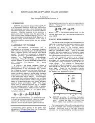
Based on the shapes of the T-r e relations 

(see Figure 2), Rosenfeld and Lensky (1998) 

defined the following five microphysical 

zones in convective clouds: 

8

1) Diffusional droplet growth zone: 

Very slow growth of cloud droplets 

with depth above cloud base, 

indicated by shallow slope of dr e /dT. 

2) Droplet coalescence growth zone: 

Large increase of the droplet growth 

rate dr e /dT at T warmer than 

freezing temperatures, indicating 

rapid cloud-droplet growth with 

depth above cloud base. Such rapid 

growth can occur there only by drop 

coalescence. 

3) Rainout zone: A zone where r e 

remains stable between 20 and 25 

m, probably determined by the 

maximum drop size that can be 

sustained by rising air near cloud 

top, where the larger drops are 

precipitated to lower elevations and 

may eventually fall as rain from the 

cloud base. This zone is so named, 

because droplet growth by 

coalescence is balanced by 

precipitation of the largest drops 

from cloud top. Therefore, the 

clouds seem to be raining out much 

of their water while growing. The 

radius of the drops that actually rain 

out from cloud tops is much larger 

than the indicated r e of 20-25 m, 

being at the upper end of the drop 

size distribution there. 

4) Mixed phase zone: A zone of large 

indicated droplet growth rate, 

occurring at T

T [ o C] 

-40 

-30 

-20 

General 

-10 

Mixed Phase 

0 

Rainout 

10 

Coalescence 

Diffusional growth 

20 

0 5 10 15 20 25 30 35 

[ m] 

r 

eff 

Glaciated 

Figure 2: The classification scheme of 

convective clouds into microphysical zones, 

according to the shape of the T-r e relations 

(after Rosenfeld and Woodley, 2003). The 

microphysical zones can change 

considerably between microphysically 

continental and maritime clouds, as 

illustrated in Figure 6 of Rosenfeld and 

Woodley, 2003. 

Alternatively, a cloud with an extremely 

large number of small droplets, such as in a 

pyro-Cb (See example in Figure 11 of 

Rosenfeld et al., 2006a), can occur entirely 

in the diffusional growth zone up to the 

homogeneous glaciation level even if it does 

not have very strong updrafts. In any case, a 

deep (> 3 km) zone of diffusional growth is 

indicative of microphysically continental 

clouds, where smaller r e means greater 

heights and lower temperatures that are 

necessary for the transition from diffusional 

to the mixed phase zone, which is a 

manifestation of the onset of precipitation. 

This is demonstrated by the model 

simulations shown in Figures 4 and 5 in 

Rosenfeld et al. (2007). Observations of 

such T-r e relations in cold and high-base 

clouds over New Mexico are shown in 

Figure 1. 

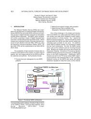
Figure 3B illustrates the fact that a 

highly microphysically continental cloud 

with a warm base (e.g., >10°C) has a deep 

zone of diffusional cloud droplet growth 

even for weak updrafts (line A in Figure 3B 

and Figure 4a). The onset of precipitation is 

manifested as the transition to the mixed 

phase zone, which occurs at progressively 

greater heights and colder temperatures for 

clouds with stronger updrafts (line B in 

Figure 3B and Figure 4b). The glaciation 

temperature also shifts to greater heights and 

colder temperatures with increasing 

updrafts. From the satellite point of view the 

cloud is determined to be glaciated when the 

indicated r e reaches saturation. This occurs 

when the large ice crystals and 

hydrometeors dominate the radiative 

signature of the cloud. Some supercooled 

water can still exist in such a cloud, but most 

of the condensates are already in the form of 

large ice particles that nucleated 

heterogeneously and grew by riming and 

fast deposition of water vapor that is in near 

equilibrium with liquid water. Such was the 

case documented by Fridland et al. (2004) in 

convective clouds that ingested mid 

tropospheric CCN in Florida, where 

satellite-retrieved T-r e relations indicated a 

glaciation temperature of -29°C (not 

shown). 

Further invigoration of the clouds would 

shift upward the onset of mixed phase and 

glaciated zones, but glaciation occurs fully 

and unconditionally at the homogeneous 

glaciation temperature of -38°C. Any liquid 

cloud drops that reach to this level freeze 

homogeneously to same-size ice particles. If 

most cloud water was not rimed on ice 

hydrometeors, it would have a radiative 

impact on the retrieved effective radius and 

greatly decrease the r e of the glaciated cloud, 

as shown in line C of Figure 3B. Yet 

additional invigoration of the updraft would 

further shift upward and blur the onset of the 

precipitation, and reduce the r e of the 

10

T [ o C] 

T [ o C] 

-50 

-40 

-30 

A 

A. Maritime, Weak updraft 

B. Maritime, Moderate updraft 

C. Maritime, Strong updraft 

D. Maritime, Severe 

E. Extreme 

(Rosenfeld and Gutman, 1994). The 

horizontal line at T=-38°C represents the 

homogeneous freezing isotherm. The left 

panel is for microphysically maritime clouds 

with low and warm bases and small 

concentrations of CCN, and the right panel 

is for clouds with high CCN concentrations 

or high and cold bases. In reality most cases 

occur between these two end types. 

-20 

-10 

0 

10 

20 

E 

B 

A 

B 

A 

0 5 10 15 20 25 30 35 

D 

C 

r 

e 

[ m] 

A. Cont, Weak updraft 

B. Cont, Moderate updraft 

C. Cont, Strong updraft 

D. Cont, Severe updraft 

E. Cont, Extreme updraft 

F. Cont Cold base strong 

-50 

-40 

-30 

-20 

-10 

0 

10 

20 

B 

F 

0 5 10 15 20 25 30 35 

r 

e 

E 

D 

C 

B 

[ m] 

A 

Figure 4a: Same as Figure 1, but for a nonsevere 

convective storm. The image is based 

on the NOAA-AVHRR overpass on 28 July 

1998, 20:24 UTC, over a domain of 

232x222 AVHRR 1-km pixels. The cloud 

system is just to the north of the Florida 

Panhandle. Note the rapid increase of r e 

towards an early glaciation at -17°C. This is 

case #9855 (see Appendix), with 

Tbase=20°C, Rbase=8 µm, T14=-5°C, TL=- 

18°C, dTL=38°C, Tg=-20°C, Rg=33.5µm 

(See parameter definitions in Figure 5). 

Figure 3: A conceptual model of the way T- 

r e relations of convective clouds are affected 

by enhanced updrafts to extreme values. The 

vertical green line represents the 

precipitation threshold of r e =14 µm 

glaciated cloud above the -38°C isotherm, 

until the ultimate case of the most extreme 

updraft, where the T-r e profile becomes 

nearly linear all the way up to the 

homogeneous freezing level. This situation 

is illustrated by line E in Figures 3A and 3B 

and in Figures 4c-4e. 

11

dTL=34°C, Tg=-27°C, Rg=32.4 µm (See 

parameter definitions in Figure 5). 

Figure 4b: Same as Figure 1, but for three 

hail storms. The image is based on the 

NOAA-AVHRR overpass on 5 March 1999, 

21:32 UTC, at a domain of 220x300 

AVHRR 1-km pixels. The cloud system is 

near the eastern border of Oklahoma. The 

locations of reported hail (0.75-1.75 inch) 

are marked by small triangles. Note the deep 

supercooled layer with glaciation 

temperature of about -25 for the median r e 

(denoted by the bottom of the vertical red 

line), and less than -30°C for the smallest r e . 

This is case #9901 with Tbase=8°C, 

Rbase=5 µm , T14=-12°C, TL=-26°C, 

Figure 4c: Same as Figure 1, but for a 

tornadic storm with 4.5 inch hail. The image 

is based on the NOAA-AVHRR overpass on 

29 June 2000, 22:21 UTC, over a domain of 


occurred in southwestern Nebraska. The 

location of a reported F1 tornado at 23:28 is 

marked by a rectangle. Note that the tornado 

occurred in a region that had little cloud 

development 68 minutes before the tornadic 

event. This demonstrates that there is 

predictive value in the cloud field before any 

of the clouds reach severe stature. A hail 

swath on the ground can be seen as the dark 

purple line emerging off the north flank of 

the storm, oriented NW-SE. Two hail gushes 

are evident on the swath near the edge of the 

storm. The precipitation swath appears as 

darker blue due to the cooler wet ground. 

Note the linear profile of the T-r e lines, and 

the glaciation occurs at the small r e =25 µm, 

in spite of the very warm cloud base 

temperature near 20°C. This is case #0046 

with Tbase=8°C, Rbase=5.5 µm, T14=- 

21°C, TL=-31°C, dTL=39°C, Tg=-32°C, 

12

Rg=20.6 µm (See parameter definitions in 

Figure 5). 

dTL=55°C, Tg=-38°C, Rg=23.9 µm (See 

parameter definitions in Fig. 5). 

Figure 4d: Same as Figure 1, but for a 

tornadic storm with 2.5 inch hail. The image 

is based on the NOAA-AVHRR overpass on 

30 April 2000, 22:14 UTC, over a domain of 


occurred just to the SE of the Texas 

panhandle. The location of a reported F3 

tornado at 22:40 is marked by a rectangle. 

Note the very linear profile of the T-r e lines, 

and the glaciation occurs at the small r e =25 

µm, in spite of the very warm cloud base 

temperature of near 20°C, as in Figure 4d. It 

is particularly noteworthy that this T-r e is 

based on clouds that occurred ahead of the 

main storm into an area through which the 

storm propagated. The same is indicated in 

Fig. 8d, but to a somewhat lesser extent. 

This is case #0018 with Tbase=18°C, 

Rbase=4.4 µm, T14=-15°C, TL=-37°C, 

Figure 4e: Same as Figure 1, but for a 

tornadic storm with 1.75 inch hail. The 

image is based on the NOAA-AVHRR 

overpass on 20 July 1998, 20:12 UTC, over 

a domain of 262x178 AVHRR 1-km pixels. 

The cloud occurred in NW Wisconsin. The 

locations of reported F0 tornadoes are 

marked by rectangles. Note the large r e at 

the lower levels, indicating microphysically 

maritime microstructure, followed by a very 

deep mixed phase zone. Very strong 

updrafts should exist for maintaining such a 

deep mixed phase zone in a microphysically 

maritime cloud, as illustrated in line C of 

Fig. 3A. This is case #9847 with 

Tbase=16°C, Rbase=8 µm, T14=8°C, TL=- 

31°C, dTL=47°C, Tg=-32°C, Rg=27.8 µm 

(See parameter definitions in Fig. 5). 

2.4 T-r e Relations of Severe 

Convective Storms in Clouds with 

Large Drops 

Line A in Fig. 3A is similar to the 

scheme shown in Fig. 2, where a 

microphysically maritime cloud with weak 

updrafts develops warm rain quickly and a 

rainout zone, followed by a shallow mixed 

phase zone. When strengthening the updraft 

13

(line B), the time that is needed for the cloud 

drops in the faster rising cloud parcel to 

coalesce into warm rain is increased. 

Consequently, the rainout zone is reached at 

a greater height, but the onset of the mixed 

phase zone is anchored to the slightly 

supercooled temperature of about -5°C. This 

decreases the depth of the rainout zone. The 

greater updrafts push the glaciation level to 

colder temperatures. Additional invigoration 

of the updraft (line C) eliminates the rainout 

zone altogether and further decreases the 

glaciation temperature, thus creating a linear 

T-r e line up to the glaciation temperature. 

Even greater updrafts decrease the rate of 

increase of r e with decreasing T, so that the 

glaciation temperature is reached at even 

lower temperatures. It takes an extreme 

updraft to drive the glaciation temperature to 

the homogeneous glaciation level, as shown 

in lines D and observed in Fig. 4f. 

Most cases in reality occur between the 

two end types that are illustrated 

schematically in Fig. 3. Examples of T-r e 

lines for benign, hailing and tornadic 

convective storms are provided in Fig. 4. It 

is remarkable that the T-r e relations occur 

not only in the feeders of the main clouds, 

but also in the smaller convective towers in 

the area from which the main storms appear 

to propagate (see Figures 4e and 4f). This 

does not imply that the smaller convective 

towers and the upshear feeders have updraft 

speeds similar to the main storms, because 

these core updrafts at the mature stage of the 

storms are typically obscured from the 

satellite view. However, it does suggest that 

the satellite inferred updraft-related 

microstructure of those smaller clouds and 

feeders is correlated with the vigor of the 

main updraft. This has implications for 

forecasting, because the potential for severe 

storms can be revealed already by the small 

isolated clouds that grow in an environment 

that is prone to severe convective storms 

when the clouds are organized. 

Based on the physical considerations 

above it can be generalized that a greater 

updraft is manifested as a combination of 

the following trends in observable T-r e 

features: 

Glaciation temperature is reached at 

a lower temperature; 

A linear T-r e line occurs for a greater 

temperature interval; 

The r e of the cloud at its glaciation 

temperature is smaller. 

These criteria can be used to identify 

clouds with sufficiently strong updrafts to 

possess a significant risk of large hail and 

tornadoes. The feasibility of this application 

is examined in the next section. 

2.5 The Roles of Vertical Growth Rate 

and Wind Shear in Measuring T-r e 

Relations 

Severe convective storms often have 

updrafts exceeding 30 ms -1 . At this rate the 

air rises 9 km within 5 minutes. The tops 

form anvils that diverge quickly, and 

without strong wind shear the anvil obscures 

the new feeders to the convective storm, 

leaving a relatively small chance for the 

satellite snap shot to capture the exposed 

tops of the vigorously growing convective 

towers. Therefore, in a highly unstable 

environment with little wind shear the T-r e 

relations are based on the newly growing 

storms and on the cumulus field away from 

the mature anviled storms. An example of 

moderate intensity little-sheared convection 

is shown in Fig. 4a. 

When strong wind shear is added, only 

strong and well organized updrafts can grow 

into tall convective elements that are not 

sheared apart. The convective towers are 

tilted and provide the satellite an opportunity 

14

to view from above their sloping tops and 

the vertical evolution of their T-r e relations 

(see examples in Figs. 4b and 4d). In some 

cases the strong divergence aloft produces 

an anvil that obscures the upshear slope of 

the feeders from the satellite view. Yet 

unorganized convective clouds that often 

pop up in the highly unstable air mass into 

which the storm is propagating manage to 

grow to a considerable height through the 

highly sheared environment and provide the 

satellite view necessary to derive their T-r e 

relations. Interestingly and importantly, the 

T-r e relations of these pre-storm clouds 

already possess the severe storm 

microphysical signature, as evident in Fig. 

4e. Without the strong instability these deep 

convective elements would not be able to 

form in strong wind shear. Furthermore, 

often some of the horizontal momentum 

diverts to vertical in a sheared convective 

environment. Weisman and Klemp (1984) , 

modeling convective storms in different 

conditions of vertical wind shear with 

directional variations, showed that updraft 

velocity is dependent on updraft buoyancy 

and vertical wind shear. In strong shear 

conditions the updrafts of long-lived 

simulated supercell storms interacted with 

the vertical wind shear and this interaction 

resulted in a contribution of up to 60% of 

the updraft strength. Furthermore, Brooks 

and Wilhelmson (1990) showed, from 

numerical modeling experiments, an 

increased peak updraft speed with increasing 

helicity. Therefore, to the extent that wind 

shear and helicity enhance the updrafts, the 

severe storm microphysical signature 

inherently takes this into account. 

2.6 The Potential Use of the T-r e 

Relations for the Nowcasting of Severe 

Weather 

2.6.1 Parameterization of the T-r e 

relations 

The next step was the quantitative 

examination of additional cases, taken from 

AVHRR overpasses that occurred 0-75 

minutes before the time of tornadoes and/or 

large hail in their viewing area anywhere 

between the US east coast and the foothills 

of the Rocky Mountains. The reports of the 

severe storms were obtained from the 

National Climate Data Center 

(http://www4.ncdc.noaa.gov/cgiwin/wwcgi.dll?wwEvent~Storms). 

For 

serving as control cases, visibly well defined 

non-severe storms (i.e., without reported 

tornado or large hail) were selected at 

random from the AVHRR viewing areas. 

These control cases were selected from the 

viewing area of the same AVHRR 

overpasses that included the severe 

convective storms at distances of at least 

250 km away from the area of reported 

severe storms. The relatively early overpass 

time of the AVHRR with respect to the 

diurnal cycle of severe convective storms 

allowed only a relatively small dataset from 

the years 1991-2001, the period in which the 

NOAA polar orbiting satellites drifted to the 

mid and late afternoon hours. Unfortunately 

this important time slot has been neglected 

since that time. In all, the dataset includes 28 

cases with tornadoes and hail, 6 with 

tornadoes and no hail, 24 with hail only and 

38 with thunderstorms but no severe 

weather. The case total was 96. The total 

dataset is given in Appendix A of Rosenfeld 

et al. (2007). 

The AVHRR imagery for these cases 

was processed to produce the T-r e relations, 

using the methodology of Rosenfeld and 

Lensky (1998). The T-r e functions were 

parameterized using a computerized 

algorithm into the following parameters, as 

illustrated in Fig. 5: 

Tbase: Temperature of cloud base, which is 

approximated by the warmest point of the T- 

r e relation. 

15

dTL 

T [ o C] 

Rbase: The r e at cloud base. 

T14: Temperature where r e crosses the 

precipitation threshold of 14 um. 

TL: Temperature where the linearity of the 

T-r e relation ends upwards. 

DTL: Temperature interval of the linear part 

of the T-r e relation. Tbase - TL 

Tg: Onset temperature of the glaciated zone. 

Rg: r e at Tg. 

These parameters provide the satellite 

inferences of cloud-base temperature, the 

effective radius at cloud base, the 

temperature at which the effective radius 

reached the precipitation threshold of 14 

µm, the temperature at the top of the linear 

droplet growth line and the temperature at 

which glaciation was complete. The T-r e 

part of the cloud which is dominated by 

diffusional growth appears linear, because 

the non linear part near cloud base is 

truncated due to the inability of the satellite 

to measure the composition of very shallow 

parts of the clouds. The T-r e continues to be 

linear to greater heights and lower 

temperatures for more vigorous clouds, as 

shown schematically re in Fig. 3. 

-50 

-40 

-30 

-20 

-10 

0 

10 

20 

Tg 

TL 

T14 

Tbase 

Rg 

0 5 10 15 20 25 30 35 

Rbase r [m] 

e 

Fig. 5: Illustration of the meaning of the 

parameters describing the T-r e relations. 

These parameters were retrieved for 

various percentiles of the r e for a given T. 

The r e at a given T increases with the 

maturation of the cloud or with slower 

updrafts, especially above the height for the 

onset of precipitation, as evident in Fig. 1. 

Therefore, characterization of the growing 

stages of the most vigorous clouds in 

percentiles requires using the small end of 

the distribution of r e for any given T. In 

order to avoid spurious values, the 15 th 

percentile and not the lowest was selected 

for the subsequent analyses. The 15 th 

percentile was used because it represents the 

young and most vigorously growing 

convective elements, whereas larger 

percentiles represent more mature cloud 

elements. 

The mean results by parameter and by 

storm type were tabulated by Rosenfeld et 

al. (2007). According to the tabulations, the 

likelihood of a tornado is greater for a colder 

top of the linear zone and for a colder 

glaciation temperature. In extreme cases 

such as that shown in Fig. 4e there is little 

difference between Tg and TL because of 

what must have been violent updrafts. In 

addition, smaller effective radius at cloud 

base indicates higher probability for a 

tornadic event. 

2.6.2 Statistical evaluation using 

AVHRR 

The primary goal of the initial analyses 

making use of AVHRR polar-orbiter 

imagery was to determine whether the 

probability of a tornado or hail event might 

be quantified using the parameterized values 

of satellite retrieved T-r e relations of a given 

field of convective clouds. Doing this 

involved the use of binary logistic regression 

(Madalla, 1983), which is a methodology 

that provides the probability of the 

occurrence of one out of two possible 

events. 

16

If the probability of the occurrence of a 

tornado event is P, the probability for a nontornado 

is 1-P. Given predictors X1, X2,… 

Xi, the probability P of the tornado is 

calculated using binary logistic regression 

with the predictors as continuous, 

independent, input variables using equation 

(3): 

P 

ln x 

(3) 

1 

P 

The basic model is similar in form to 

linear regression model (Note the right side 

of the equation.), where α is the model 

constant and β is a coefficient of the 

parameter x of the model. 

The first step is calculation of P/(1-P) 

according to (3). The logistic regression was 

done in a stepwise fashion, so that the 

procedure was allowed to select the 

parameters that had the best predictive skill. 

The details of the calculations are given in 

Rosenfeld et al. (2007). The analysis 

revealed that microphysical continentality 

along with slow vertical development of 

precipitation in the clouds apparently are 

essential for the formation of tornadoes. 

Also non-tornadic hail storms can be 

distinguished from non severe storms by 

their microphysically continental nature, as 

manifested by smaller Rbase and cooler 

cloud bases. However, the tornadoes differ 

mostly from hail-only storms by having 

smaller r e aloft (lower T14), extending the 

linear part of the T-r e relations to greater 

heights (greater dTL) and glaciating at lower 

temperatures that often approach the 

homogeneous freezing isotherm of -38°C 

(lower Tg). The freezing occurs at smaller r e 

(lower Rg). All this is consistent with the 

conceptual model that is illustrated in Fig. 3. 

3.0 INITIAL TESTS OF THE 

CONCEPTS USING GOES 

IMAGERY (SBIR 1) 

The initial investigation discussed 

above, suggested that multi-spectral, polarorbiter, 

AVHRR satellite imagery could be 

used to identify clouds that had the potential 

to produce severe weather. This finding 

would have positive ramifications for severe 

weather forecasting and warning if multispectral 

Geostationary Operational 

Environmental Satellite (GOES) imagery, 

providing good temporal resolution, could 

be used for the measurements. At this point 

Dr. Woodley contacted NOAA’s Small 

Business Innovative Research (SBIR) 

program to seek support to test the 

feasibility of the concept as applied to 

GOES imagery. The goal of this SBIR Phase 

1 effort would be to determine whether 

GOES multi-spectral satellite imagery has 

potential for the short-term forecasting of 

severe weather, especially tornadoes. It 

would be predicated on the finding from 

initial analyses of multi-spectral polarorbiter 

satellite data (described herein) that 

the height profiles of cloud-particle effective 

radius, showing a deep zone of diffusion 

droplet growth, little coalescence, no 

precipitation, and delayed glaciation to near 

the temperature of homogeneous nucleation 

(~ -38 o C) are associated with tornadoes and 

hail. This would mean that a satellite-based 

severe storm signature is an extensive 

property of the clouds before storm 

outbreaks. It implied further that the 

probabilities of tornadoes and large hail 

might be obtained at lead times > 1 hour 

prior to the actual event. This would 

represent a major improvement over what is 

possible currently. Because of these 

potential payoffs, Woodley Weather 

Consultants received a SBIR Phase 1 (SBIR- 

1) award to test these concepts on GOES 

imagery. 

In making use of GOES instead of 

AVHRR satellite data it was necessary to 

trade the fine (1-km) spatial resolution 

17

obtainable from the polar orbiters once-perday 

for the degraded 4-km spatial resolution 

that is available in GOES multi-spectral 

images every 15 to 30 minutes. Upon 

comparing the two imagery sources, the 

GOES data did not seem to have a 

systematic error relative to the polar-orbiter 

AVHRR data. The main effect was losing 

the smaller sub-pixel cloud elements, which 

were primarily the lower and smaller clouds. 

Therefore, cloud base temperature could not 

be relied on quantitatively as in the AVHRR 

imagery, so that it would be necessary to 

divide the GOES scenes into two indicated 

cloud base temperature classes with a 

demarcation at 15°C. The effectiveness of 

the detection of linearity of the profiles and 

glaciation temperature was compromised to 

a lesser extent, because the cloud elements 

were already larger than the pixel size when 

reaching the heights of the highly 

supercooled temperatures. No quantitative 

assessment of the effect of the resolution 

was done in this preliminary study beyond 

merely testing the skill of the T-r e retrieved 

parameters. 

The analysis using GOES imagery was 

done only for detecting tornadoes, because 

the AVHRR analysis showed that the 

predictor parameters had more extreme 

values for tornadoes than for hail. The 

continuing research entailed the use of 

archived multi-spectral GOES imagery 

instead of polar-orbiter satellite data, which 

were used to derive the relationships. All of 

the useable old polar-orbiter data had been 

exhausted during the initial tests and there is 

no prospect of additional useable polarorbiter 

data due to the oversight of lack of a 

late afternoon slot for the polar orbiters. 

Further, imagery from a polar orbiting 

satellite is available at a given location only 

once or twice per day, which is too 

infrequent for forecasting purposes. Thus, 

the key question going into SBIR-1 effort 

was whether anything meaningful could be 

obtained by using the GOES imagery that 

provides much-enhanced temporal 

resolution at the expense of the spatial 

resolution. 

Seventeen (17) days with past tornadic 

events were examined using conventional 

weather data and archived, multi-spectral, 

GOES-10 imagery, which were obtained 

from the Cooperative Institute for Research 

in the Atmosphere (CIRA) satellite archive. 

For each case, the area of interest was first 

identified by noting severe weather reports 

from the Storm Prediction Center’s (SPC) 

website. The chosen area typically 

encompassed at least 6 central U.S. states, 

but was larger for the more extensive severe 

weather outbreaks. Data were obtained 

beginning in the morning, usually around 

1600 UTC, and extended to near sunset. 

Rapid scan imagery was not analyzed, and 

only the regular 15 to 30 minute scans were 

used. The GOES satellite imagery was 

analyzed using the T-r e profiles for multiple 

significant convective areas within the field 

of view. The T-r e parameters as defined in 

Fig. 5 were calculated for each such 

convective area. The GOES-retrieved r e 

reached saturation at 40 µm, instead of 35 

µm for the AVHRR. Other than that the T-r e 

parameters were calculated similarly. 

On the 17 case days there were 86 

analyzed convective areas, 37 of the 86 

analyzed areas had a total of 78 tornadoes. 

As in the analysis of the AVHRR data set, 

logistic regression was done in a stepwise 

fashion, so that the procedure was allowed 

to select the parameters that had the best 

predictive skill. The satellite-based 

predictors were found to be at least as good 

as the sounding-based predictors, although 

the two are only loosely correlated. The 

logistic regression parameters and 

coefficients data for the soundings and 

satellite retrieved parameters are in 

Rosenfeld et al. (2007). 

18

P 

The graphical representation of the 

probability (P) for a tornado is depicted best 

by the transformation of P to log10(P/(1-P)). 

This transformation of P is used in the 

graphical display shown in Figure 6 because 

it is important to expand the scales near P=0 

and P=1. Note that when log10(P/(1-P) = 0, 

P = 0.50. Histograms of log 10 (P/(1-P)) for 

the satellite-based logistic regression 

prediction models are shown in Figure 7. 

The top panel gives the satellite-based 

predictions for tornadic and non-tornadic 

storms, while the bottom panel gives the 

sounding-based predictions for tornadic and 

non-tornadic storms. The regression 

predictions provide good separation for the 

cases. 

1 

0.8 

0.6 

0.4 

0.2 

0 

-2 -1.5 -1 -0.5 0 0.5 1 1.5 2 

LOG10(P/(1-P)) 

Figure 6: The relations between the 

probability for an event P and the 

transformation to log10(P/(1-P)). 

The potential lead time from the 

geostationary satellite data for a severe 

weather event was assessed by Rosenfeld et 

al. (2007) for some of the most intense 

tornadoes in the data set. The satellite-based 

predictor rose some 90 minutes or even 

more before the actual occurrence of the 

tornado. In many cases it manifested itself 

with the first clouds that reached the 

glaciation level. For all the tornadic storms 

in the dataset the tornado probabilities 

exceeded 0.5 by 150 minutes before the 

occurrence of the tornado, and increased to 

0.7 at a lead time of 90 minutes. In 

comparison, the median P of the nontornadic 

storms was about 0.06. This shows 

the great ―Early-Alert‖ potential of the 

methodology. 

The overall predictive skill of the 

soundings and the GOES satellite are 

comparable, but the satellite is much more 

focused in time and space. The difference 

between the sounding and satellite based 

predictions can be better understood when 

plotting the time dependent predictors for 

tornadic cases. The sounding based predictor 

is fixed in time and space for the analyzed 

area, because there is only one relevant 

sounding that can indicate the pre-storm 

environment before the convective 

overturning masks it. The satellite predictor 

on the other hand varies and is recalculated 

independently for each new satellite 

observation. This allows the satellite based 

predictor to react to what the clouds are 

actually doing as a function of time at scales 

that are not resolved properly by the 

soundings or by models such as the Rapid 

Update Cycle (RUC). 

The association between strong updrafts, 

as inferred by the T-r e profiles, and 

tornadoes and hailstorms makes sense 

physically. The combined physical 

considerations and preliminary statistical 

results suggest that clouds with extreme 

updrafts and small effective radii are highly 

likely to produce tornadoes and large hail, 

although the strength and direction of the 

wind shear probably would be major 

modulating factors. The generation of 

tornadoes often (but not always) requires 

strong wind shear in the lowest 6 km and 

low level helicity (Davis, 2006). According 

to the satellite inferences here this might be 

helping spin up the tornadoes in storms with 

very strong and deep updrafts that reach the 

anvil level. These strong updrafts aloft are 

19

Number of Cases 

Frequency 

TornadoYN 

1 0 

TornadoYN 

1 0 

Number of Cases 

Frequency 

revealed by the linear T-r e profiles that 

extend to greater heights and r e reaching 

smaller values at the -38°C isotherm in 

tornadic versus hail storms. These inferred 

stronger and deeper updrafts in tornadic 

storms compared to hailstorms imply that in 

low CAPE and high shear environment 

some of the energy for the updrafts comes 

from converting horizontal to vertical 

momentum, as already shown by Browning 

(1964). Fortuitously, the tilting of the feeder 

and pre-storm clouds in the high shear 

tornadic storms render them easier to see by 

satellite and this facilitates the derivation of 

the T-r e profiles and the retrieval of tornadic 

microphysical signatures, as described 

above. 

50 50 

40 40 

30 

30 

20 20 

10 

10 

00 

50 

40 

30 30 

20 20 

10 10 

00 

B: Sounding prediction 

Tornadic storms 

Non-Tornadic 

-1.00 

0.00 

1.00 

2.00 

-6 -4 -2 0 2 

Log_Psond_all 

Log10(P/1-P)) 

50 50 

40 40 

30 

30 

20 20 

10 

0 

10 

0 

50 

40 

30 30 

20 

20 

10 

10 

0 

0 

A: GOES prediction 

Tornadic storms 

Non-Tornadic 

-6.0 

-4.0 

-2.0 

0.0 

2.0 

0 2 

Log_Psat_Combined 

Log10(P/1-P)) 

Figure 7: Histograms of the predictions 

log 10 (P/(1-P)) for the GOES satellite (A) and 

the sounding (B) based models. The upper 

panel is for tornadic scenes, and the lower 

panel for non tornadic areas. 

The research to this point had indicated 

that the potential of new growing deep 

convective clouds to become storms that 

produce large hail and tornadoes can be 

revealed by the satellite-retrieved vertical 

evolution of the microstructure of these 

clouds. Deep clouds composed of small 

drops in their lower parts and cool bases are 

likely to produce hail, because such clouds 

produce little warm rain and most of the 

condensate becomes supercooled water with 

relatively small concentrations of 

precipitation embryos. Large graupel and 

small hail can develop under such 

conditions. The hail becomes larger with 

greater updraft velocities at the supercooled 

levels. This can be inferred by the increased 

depth of the supercooled zone of the clouds, 

as indicated by lower glaciation 

20

temperatures. This is also manifested by an 

increase of the height for onset of significant 

precipitation, as indicated by lower T14. 

Tornadic storms, which are often 

accompanied by very large hail, are 

characterized by the parameters that indicate 

the strongest updrafts at the supercooled 

levels, which are indicated by markedly 

lower values of Tg and TL and smaller Rg 

than for hail-only storms. 

This study did not address the role of 

wind shear in tornado development. 

However, the extent that wind shear 

modulates severe storms by affecting their 

updraft speeds can be revealed by the 

methodology presented in this study. The 

helicity of the wind shear should increase 

the probability of a tornado for a given 

updraft velocity (Weisman and Klemp, 

1984; Brooks and Wilhelmson 1990; 

Rasmussen and Blanchard, 1998). A 

combination of the satellite methodology 

with soundings parameters should be more 

powerful than each method alone. The 

sounding and synoptic parameters identify 

the general areas at risk of severe weather 

and the continuous multispectral satellite 

imagery identifies when and where that risk 

is about to be realized. 

This study suggests that multispectral 

satellite data have yet untapped predictive 

skill for nowcasting of hail and mainly 

tornadic storms. This application will 

require using retrieved microstructure from 

geostationary satellites, which provide 

smaller spatial resolution (3 to 4 km at the 

sub geostationary satellite point) than the 

polar-orbiting satellites used in this study 

(1.1 km beneath the satellite) and are hence 

less useful. However, the added dimension 

of time evolution that is possible with GOES 

imagery appears to compensate for its 

poorer spatial resolution, and allows timely 

early alerts of the risk of tornadoes from the 

developing storm clouds. While this method 

appears to have useful results with the 

current GOES satellites, it is developed with 

the expectation of improved resolution with 

the next generation of geostationary 

satellites. The resolution will be 2 km for the 

GOES-R and 1-km for the high resolution 

coverage of the METEOSAT third 

generation. 

SBIR-1 had not been aimed at testing an 

operational methodology for satellite 

quantification of the risks of severe 

convective storms, but rather the testing of 

the validity of the conceptual model that will 

hopefully allow subsequent development of 

such an operational methodology using 

geostationary satellites. Therefore, the 

statistical analyses are exploratory in nature 

at this stage of the research. Although the 

small sample size does not allow a rigorous 

evaluation of the predictive skill of the 

conceptual model, it is sufficient to support 

the conceptual model. The existence of the 

severe storm signature in the pre-storm 

clouds provides us with the prospect that 

this methodology, when applied to 

geostationary multispectral satellite imagery, 

will make it possible to identify earlier than 

is possible now developing cloud areas that 

are about to become severe convective 

storms, possibly producing tornadoes and 

large hail. The clouds in this early stage 

typically have not yet developed radar 

severe storm signatures. Therefore, the 

capability of detecting the potential of 

clouds to become severe convective storms 

may provide additional lead time for more 

focused ―watch‖ areas, although with lesser 

accuracy and focus than the detection of 

severe weather that is already possible with 

radar. This method has the potential of 

filling the currently large gap between large, 

poorly focused ―watch‖ areas and 

"warnings" by providing ―Early Alerts‖ of 

severe convective storms that are actually 

observed subsequently. The challenge that 

the National Weather Service faces in 

21

coping with the severe weather threat is 

addressed in the next section. 

4.0 COPING CURRENTLY WITH THE 

SEVERE WEATHER THREAT 

Statistics from the Storm Prediction 

Center show that over 1,000 tornadoes strike 

the United States each year, making it the 

most tornado-prone country in the world. Up 

to 40 deaths per year have occurred in the 

U.S. alone over the past 10 years. The most 

notable of the tornadic events was the series 

of tornadoes that struck the Oklahoma City 

area on May 3, 1999. These were the most 

damaging in U.S. history, causing over 1 

billion dollars in damage and completely 

destroying over 2,500 structures. Although 

lives were lost in these events, excellent 

warnings from the National Weather Service 

saved many lives. Even so, NWS forecasts 

need to be improved further especially as it 

relates to ―false alarms.‖ How this can be 

done was addressed by the SBIR Phase 2 

research. Before getting into that it is 

important to put everything into the context 

of current NWS tools and procedures. 

After completion of NWS’ 

Modernization during the l990’s, it moved 

from a tiered office structure of 320 fulltime 

and part-time local NWS offices to a 

structure with about 122 modernized, fulltime 

weather forecast offices (WFOs—for 

further details on the NWS Modernization, 

see Friday (l994). Each office is fully 

equipped with the latest technologies for 

observing, forecasting, and warning of 

severe thunderstorms and their attendant 

hazardous phenomena, such as tornadoes, 

large hail, heavy rain, and high winds or 

―downbursts.‖ The key new technologies 

now implemented nationwide as part of 

NWS Modernization include WSR-88D 

Doppler weather radar (a network of 165 

radars run collaboratively by the NWS, 

DoD, and DoT), Automated Surface 

Observing Systems (ASOS) at over 1,200 

sites, GOES-10 and 12 (the new generation, 

with greater spatial resolution, more 

frequent imaging, and more image channels, 

including multi-spectral data), and most 

important, the Automated Weather 

Interactive Processing System (AWIPS) 

{one at each WFO and several additional at 

each of the National Centers for 

Environmental Prediction (NCEP, including 

SPC) and River Forecast Centers}. AWIPS 

is a computer workstation and display 

system and is crucial to integrating the vast 

amount of data that flows from WSR-88D, 

ASOS, GOES-10 and 12, wind profilers, 

and other present and planned observing 

systems (e.g., NPOESS). See also Smith et 

al., (1999), and Wilson et. al, (1999) for 

more details. AWIPS also provides the 

computer and communications power to 

prepare short-term forecasts and warnings of 

all hazardous weather, especially severe 

thunderstorms and tornadoes. 

Tornado prediction has improved 

dramatically over the past 25 years. This is 

attributable to the continuous, high 

resolution coverage of GOES satellites; 

improved use of radar, forecaster training, 

and local storm spotter networks, and 

awareness campaigns. 

The conceptual models on how 

tornadoes form have evolved from a simple, 

random bathtub vortex approach to one 

where a parent circulation, termed a 

mesocyclone, sometimes develops at 

midlevels in a severe supercell thunderstorm 

prior to tornado touchdown. However, the 

l994-95 Project VORTEX (Rasmussen et al, 

l994) has found that large, intense tornadoes 

may spin-up in the boundary layer initially 

without any mesocyclone in the parent 

storm. 

The newer ETA (now NAM) and rapid 

update cycle (RUC) mesoscale models 

22

eing run at NCEP are providing severe 

storm forecasters with higher resolution and 

more accurate predicted fields of the critical 

atmospheric parameters that lead to severe 

thunderstorm and tornado development. 

These models can also be used to portray 

forecasted atmospheric soundings at any 

location out to 48 hrs. Moreover, the new 

Weather and Research Forecast Model 

(WRF) is being tested in real-time at 

resolutions down to 4-10 km, and shows 

remarkable skill in some tornadic stormdevelopment 

scenarios. The WRF is now 

running operationally at NCEP as the NAM 

Model at 13 km resolution. 

There have also been significant 

improvements in warning for tornadoes over 

the past 25 years. In l978, the probability of 

detection (POD) score for tornadoes for 

NWS was only 0.22. In other words, 22% of 

the tornadoes had warnings that preceded 

their initial impacts. Warning lead-times 

averaged just 3 min before impact. In l998, 

the POD for tornado warnings had risen to 

0.65. The average lead-time for those events 

that had a prior tornado warning was 11 

min. The major factor in this increase is the 

installation and skilled use of the WSR-88D 

radars during the 1990’s and early 21 st 

Century. However, the false alarm ratio in 

recent years has risen to a national average 

of about 0.75. The total number nationally 

of severe thunderstorm and tornado 

warnings has also risen to 10,000-12,000 

per year. This means that while forecasters 

are doing a better job in detecting and 

warning about tornadoes with greater leadtimes, 

they are issuing warnings too often 

and appear to be over warning the public. 

This could cause problems later with public 

credibility and response (Golden and 

Adams, 2000); however, the extent to which 

high false alarm ratios influence warning 

response behavior has not been 

systematically researched by social 

scientists. NWS seems to be moving from 

the era of ―detected‖ warnings (warnings 

based on detecting existing tornadoes) to the 

era of ―predictive‖ warnings (warnings 

based on forecasts of tornado formation). 

Generating such predictive warnings is the 

essence of the SBIR Phase 2 (SBIR-2) 

research effort. This, combined with 

improvements in warning coordination and 

communication, has lead to the reduction in 

morbidity and mortality for tornadoes. 

Continued improvement is expected. 

The tornado information communication 

paradigm used by NWS includes several 

types of forecast and warning products. 

Outlooks for severe convective weather (i.e., 

severe thunderstorms) are issued 1-2 days in 

advance from SPC. An example of a 

convective weather outlook for May 10, 

2008, a day of interest in the Oklahoma tests 

of the methodology, is given in Figure 8. 

The storm reports for this day, which were 

available the following morning, are given 

in Figure 9. The reports of severe weather 

agreed well with the convective outlook for 

this day. 

The convective outlooks are the first 

notifications of the threat to both local NWS 

offices and local emergency management 

officials. These outlooks may be followed 

by the issuance of tornado watches that are 

issued currently for large areas that have a 

significant potential to experience severe 

thunderstorms capable of producing 

tornadoes. This is the first official 

notification to the public of a significant 

threat. The SPC watch process is discussed 

in more detail below. Shorter range 

outlooks are issued in the morning during 

tornado season by local NWS offices to 

describe the likelihood of severe weather in 

their forecast areas. This includes 

information on type of severe weather, 

general locations within a county warning 

area, and time frames. As events unfold, 

short-term forecasts are issued on a frequent 

23

―as needed‖ basis as the severe weather 

begins to form. When a tornado is believed 

to be imminent, based on radar or other 

detection technology, or is spotted and 

reported, a tornado warning is issued. The 

warning contains specific language on areas 

at risk, time frames, specific hazards, 

recommended protective behavior for those 

at risk, and the office issuing the warning. It 

is also important to note that NWS’ 

approach to the warning process for 

tornadoes is a weather-warning partnership 

with local emergency managers, private 

forecasters and the news media. The SBIR-2 

tests fit nicely into this scenario. 

The proposed multi-spectral satellite 

tornado detection and warning technique is 

highly complementary to other sources of 

data used both in SPC’s tornado watches 

and WFOs’ tornado warnings. In the former, 

SPC typically issues tornado watches based 

on mesoscale diagnostic and analysis 

products, as well as NWP model data, 

especially the RUC and NAM. Tornado 

watches are now typically 24,000 sq mi in 

size (see Table 1) and last for 6-8 hours. Of 

great interest is the fact that only slightly 

more than half of all tornado watches are 

verified by at least one tornado subsequently 

within them; moreover, only slightly more 

than half of all reported tornadoes fall within 

a tornado watch. There is clearly much 

opportunity for improvement in tornado 

watches. However, SPC does a much better 

job of catching significant tornadoes within 

one of their tornado watch areas (79%). 

Finally, about 90% of all reported tornadoes 

fall within either a severe thunderstorm or a 

tornado watch. 

Figure 8. The convective weather outlook 

for the United States on May 10, 2008 

issued by the Storm Prediction Center (SPC) 

Figure 9. The SPC Storm Reports for May 

10, 2008 as updated on May 20, 2008. 

The lead-time on some tornado watches 

is sometimes only about one-half hour. 

Thus, if delivery of multi-spectral satellite 

data can be made timelier, it should 

contribute to increased lead-time of tornado 

watches, as well as higher skill in capturing 

tornadoes within watch areas. It should also 

contribute to more accurate ―convective 

outlook‖ products issued during each 

morning by SPC to indicate risk areas of 

severe weather over the entire U.S. 

(especially for those tornado outbreak cases 

when supercells are developing explosively 

and early). 

24

One good example of prototype 

technologies that have improved warning 

issuance is the Warning Decision Support 

System (WDSS), developed by Eilts and 

colleagues at NOAA’s National Severe 

Storms Laboratory (Eilts, l997; Johnson et 

al., l997). It was developed to meet the 

needs of forecasters in WFO’s to help them 

make timely, effective, and efficient 

warning decisions (for severe weather, 

tornadoes and flash floods). WDSS is a 

combination of a number of automated 

algorithms that utilize Doppler radar data to 

automatically detect and predict severe 

weather phenomena, and an innovative color 

display that was designed specifically to 

meet the needs of weather forecasters. The 

severe weather detection and prediction 

algorithms utilize image processing, 

artificial intelligence, neural networks, 

expert system, and fuzzy logic techniques to 

detect weather phenomena and to predict the 

occurrence of severe weather at the surface 

0-30 min in advance. 

WDSS was extensively field tested at 

several NWS field offices over the latter half 

of the l990’s. It was also selected to support 

the l996 Summer Olympics in Atlanta. Most 

important, the WDSS system was deployed 

and used by the Oklahoma City, OK 

forecasters during the massive May 3, 1999 

Central Oklahoma tornado outbreak. During 

that outbreak, the OKC WFO issued 116 

separate warnings with better-than-average 

lead-times of 20-60 min. The OKC 

Meteorologist-in-Charge credited the 

warnings’ success and relatively low 

number of fatalities to four major system 

components: (1) The WSR-88D radar 

network; (2) the new AWIPS, especially its 

warning generation software; (3) WDSS 

used as an adjunct to AWIPS; (4) the close 

coordination among WFOs, local media, and 

local/state emergency management offices. 

We should also note that key WDSS 

functionality has subsequently been 

incorporated into the AWIPS systems at 

WFOs nationwide, primarily though the 

SCAN (System for Convection Analysis and 

Nowcasting--Smith et. al, l999) program. 

Thus, there is a precedent for the 

development and use of prototype 

technologies to improve severe weather 

forecasts. This is the goal of SBIR- 2 for 

much of the United States, including those 

areas that rarely experience tornadoes such 

as that west of the Rocky Mountains. Some 

of the cases analyzed in SBIR-1 were over 

the Rockies and Western U.S., where 

NEXRAD coverage is sparse and the radar 

antennas are at high elevations above cloud 

base. The technique also seems to have 

superior skill over NEXRAD alone in those 

cases when the NEXRAD didn’t detect any 

mesocyclones in the parent storm. The Salt 

Lake City, Eastern Wyoming and Colorado 

cases show great promise in improving 

tornado warning skill (PODs and lead-times) 

and reducing the current high false-alarm 

rate for warnings based primarily on 

NEXRAD. Somewhat surprisingly, the 

technique demonstrates skill in forecasting 

those storms about to produce even weak to 

moderate tornadoes (F0-F2’s), and it can 

anticipate both small numbers of tornadoes 

as well as major outbreaks. Nationally, the 

False-Alarm-Rate for all tornado warnings 

still averages about 75%, and there has been 

a disconcerting decrease in the POD during 

the past year. 

It now must be shown in SBIR-2 how 

the technique can be automated to produce 

useful near-real-time products for the SPC 

and WFO forecasters to use as a 

complement to their other operational tools. 

TABLE 1: SPC Tornado Watch 

Statistics (averaged over ten years, l995- 

2004) 

25

57% - Tornado watches verified by a 

tornado 

92% - Thunderstorm and tornado watches 

verified by either a severe thunderstorm or 

tornado report 

54% - Tornadoes in a tornado watch 

79% - Significant tornadoes in a tornado 

watch 

71% - Tornadoes in either a tornado or 

severe thunderstorm watch 

90% - Significant tornadoes in either a 

tornado or severe Thunderstorm watch 

79% - Significant tornadoes (F2-F5) 

in a tornado watch 

60% - Severe thunderstorm or 

tornado in either a severe 

thunderstorm or tornado watch 

72% - Significant Severe 

Thunderstorm (hail>2",Gust> ) or 

significant tornado in tornado or 

severe thunderstorm watch 

23,773 mi 2 - median area tornado 

watch 

22,967 mi 2 - median area tornado 

and severe thunderstorm watches 

These are all 10 year averages (1995- 

2004) of the parameters computed for each 

individual year. Lead time is from the time a 

watch is publicly issued to the first event 

within the watch. It must be remembered 

that there is a coordination period, usually of 

about 17 minutes, between the time the 

decision to issue a watch is made and the 

time the watch is publicly issued. Since 

follow-on watches (i.e., those over 

downstream areas immediately adjacent to 

the watch) are included in the lead time 

computations, these numbers are really low 

estimates. 

Starting in 2005, SPC began verifying 

watches by individual counties. When this is 

done, we see that the average lead time to 

the first tornado in each county in a tornado 

watch is 3.3 hours and the average lead time 

to the first severe thunderstorm report in 

each county is 3 hours. 

While the ideal would be for every tornado 

to be in a tornado watch, the state of the 

science makes it a realistic goal to have all 

occurrences of 3 or more tornadoes within 

an area of 25,000 mi 2 of any intensity or of 

any strong or violent tornado (F2-F5) in a 

tornado watch. 

These materials demonstrate that 

addressing the severe weather threat in the 

United States is a difficult task, and anything 

that would make the job easier certainly 

would be welcome. The Early Alert Method 

for severe convective weather was proposed 

and developed under SBIR 2 with this in 

mind, and plans were being made for realtime 

tests of the methodology during the 

tornado season of 2008. Before this could be 

done, however, the method had to be 

automated for real time application. How 

this was done is addressed in the next 

section of this report. 

5.0 AUTOMATING THE EARLY 

ALERT METHODOLOGY 

Considerable progress had been made on 

the SBIR-2 calls for automation of the 

severe storm detection algorithm during the 

first year of the SBIR-2 effort. During the 

work it was noted that the imagery from 

GOES-12 is inferior for project purposes to 

that from GOES-10 and GOES-11, because 

the 12 µm infrared channel had been 

replaced by a single CO 2 channel. Thus, a 

way had to be found to replace the 12 

micron infrared channel with the CO 2 

channel by developing a method to mask the 

broken and thin clouds. Of most 

consequence was the automation of the 

Rosenfeld analysis methodology and its 

incorporation into the overall system. This 

was a major milestone. Quantification of the 

severe weather threat was done by 

26

calculating Early Alert scores using the 

scoring scheme presented Table 2. The 

focus was then on improving and testing the 

overall system. 

The full story of how the Rosenfeld 

Early Alert Methodology was automated 

and tested is told in Appendix A of Woodley 

et al. (2008) by Guy Kelman, who did most 

of the work. It is provided there for 

documentation purposes and for scientific 

posterity. 

Table 2 Procedure for the Calculation of 

Severe Storm Scores by Satellite Image 

(Now done in the Automated Algorithm) 

For the satellite field of view the 

following parameters are calculated for each 

pixel of 4x4 km: 

1. Determine cloud top temperature 

(T). 

2. Visible reflectance is corrected for 

the solar zenith angle. 

3. Statistics of the HRV (mean, 

variances, skewness) 

4. Texture roughness parameters (based 

on the HRV channel) 

5. Apply the cloud mask. 

6. Calculate cloud-top-particle effective 

radius (Re). 

The whole satellite field is scanned 

sequentially with windows of 26x26 4-km 

pixels. Thus, each score window is roughly 

100 km on a side. The window is advanced 

at steps of half of a window (13 pixels), both 

east-west and north-south. The window size 

is a parameter that can accept any even 

value. 

For each window the T-Re relations are 

calculated as follows: 

1. For each 1°C temperature interval a 

Re value is assigned. For each 1°C 

temperature interval there are three 

possibilities: 

a. There is no cloudy pixel that 

has that T. The Re for that T 

remains missing. 

b. There is one cloudy pixel 

with that T. The Re is taken 

from this same cloudy pixel. 

c. There is more than 1 cloudy 

pixel. The Re values are 

sorted and, for example, the 

30 th percentile of the Re 

might be matched with that 

T. The percentile value (30) 

is a parameter that can be set 

as any number between 0 and 

100. 

2. The T-Re function undergoes 

running averaging, where Re of each 

T value is averaged with its 

immediate neighbors in the T 

dimension, weighted by the number 

of pixels that contribute to each T 

1°C interval. 

3. Further averaging with its immediate 

neighbors points which are local 

maxima in values of Re. If Re of the 

immediate neighbor is missing, 

average with the next one instead, if 

not missing too. 

For each calculation window the set of 

computed T-Re relations are used to 

determine the ―severe storm score‖ for that 

window. The score is a multiplication of 

several parameters having values between 0 

and 1. The larger the score the greater the 

probability there is of a severe storm. If a 

parameter is 0, it means that it alone can 

disqualify the window from being a 

candidate for a severe storm. A value of 1 

means maximum probability based on this 

parameter alone, but it might be overridden 

by multiplication with another parameter 

with a 0 value. The overall score is the n th 

root of the multiplication of the n values of 

27

the individual parameters, multiplied by 

1000. 

The scores of individual parameters are 

computed as follows: 

-40 

-35 

T 0 

= -6 - 0.7Re 

1. Tb, cloud base temperature. Tb is T 

of the warmest cloudy element in the 

T-Re table. For reducing distortion 

due to ground effects, the warmest T 

is rejected if it has a Re greater than 

the Re of its neighbor colder element 

and the number of pixels composing 

it is smaller than the number of 

pixels composing the neighboring 

element. Then Tb is replaced with 

the colder neighboring T. This test is 

also applied on the new Tb and so on 

until it is no longer satisfied. The 

score is calculated as Tb/10. If the 

result is 0, then Tb=1. 

2. Ttop, the coldest cloudy T in the 

window. 

Ttop_score=-(Ttop-(-38))/12. 

if(Ttop_score1)Ttop_score=1 

3. ReGlac, the Re at the glaciation 

temperature. 

ReGlac_score=(43-ReGlac)/20. 

4. Tg, glaciation temperature. Tg must 

be between -1 and -40°C. If Tg is 

warmer than -40°C it is assigned as 

the warmest T that had reached the 

largest values of Re in the T-Re 

profile. 

Tg must be smaller than To as 

depicted by the ReGlac-To relations 

in Figure 10. 

T 0 

-30 

-25 

-20 

-15 20 25 30 35 40 

ReGlac 

Figure 10: The maximum allowed 

Tg for a given ReGlac. 

The Tg_score=(To-Tg)/(To+40) 

If the score is

where SlopeLG is the slope between 

Tg and Tlinmin, and SlopeTL is the 

slope between Tlinmin and Tb. 

SlopeChange_score=(0.6- 

SlopeChange)/0.6 

8. Slopemin is the minimum slope 

between Tb-5 and T=-40°C. 

Slopemin_score equals 1 except for 

the case that Slopemin

office (Room 3221) to connect with the flow 

of GOES 11 and GOES 12 imagery and the 

RUC data that was set up for us by Bob 

Rabin of NSSL. How this was done is 

explained by Guy Kelman in some detail in 

Appendix A of Woodley et al. (2008). 

The satellite data were fed into a laptop 

that was nick-named GIZMO and then it 

was split off to a MAXTOR hard drive 

where the data were archived and to another 

notebook computer nick-named ELWOOD 

where the data could be manipulated and 

monitored. This is where the real-time data 

could be displayed for Early Alerts on a 

large monitor and then converted manually 

to PNG files by hitting the ―snapshot‖ 

button on the computer monitor. This PNG 

snapshot archive for the day remained on the 

computer until the evening when it was 

removed in preparation for the next day. To 

obtain the PNG files for previous days it was 

necessary to retrieve them from the archive 

using a special procedure. 

It took several days to get the system up 

and operating. Dr. Rosenfeld joined Guy 

Kelman in Norman on April 13 th and then 

left on April 20 th for the joint AMS/WMA 

meetings in Westminster, Colorado. On 

April 25 th Dr. Rosenfeld and his wife Malka 

left the Woodley home in Colorado to return 

to Israel. Dr. Woodley then traveled by air to 

Norman, Oklahoma on April 28 th , arriving 

mid-day. He rented a car and drove to the 

Residence Inn in Norman, where he 

registered for an extended stay. Dr. Woodley 

then went to the National Weather Center 

off HWY 9 on Jenkins Street to join Guy 

Kelman, where the EAP effort had been 

provided office space. 

It took a while for Dr. Woodley to get 

familiar with the system that Mr. Kelman 

had devised and implemented. It involved 

pulling the processed images onto the 

monitor screen as they became available. 

These were then snap-shotted into the 

system to create a PNG file and then they 

were examined for the existence of Early 

Alert boxes. When he hit the snap-shot 

button on a given file it was posted on the 

EAP website at (http://severe-storms.net). It 

was intended that ultimately the forecaster 

would go to this site to see the latest Early 

Alert from the methodology. The problem 

was that the score numbers within the Early 

Alert boxes were illegible even on the 

mapped product. This needed work. If Dr. 

Woodley forgot to hit the snap-shot button 

no PNG file was created and it would have 

to be created later from the archive. An 

example of the thousands of images 

generated during the real-time tests of the 

methodology is provided in Figure 11 for a 

processed image from GOES-11 at 2030 

UTC on April 23, 2008. The Early Alert 

boxes are superimposed on the image. The 

severe storm scores are shown within the 

boxes. 

Before Guy Kelman and his family (wife 

and 4 children) left Oklahoma on the 

afternoon of May 2, 2008, Dr. Rosenfeld 

had discovered a minor error in his 

methodology that he eliminated over the 

course of a couple of days. After this 

problem was eliminated the old cases had to 

be rerun. After they had been rerun they had 

to be interfaced with a new program written 

by Guy that permitted the comparison of the 

locations of severe weather as documented 

by the Storm Prediction Center with the 

Early Alert boxes generated by the 

Rosenfeld satellite methodology. In the 

versions shown by Guy to Dr. Woodley a 

map showing the position and type of severe 

storm reports over the past half-hour or hour 

was shown. Then he went back 2 hours prior 

to the ending time of the storm plot and 

progressively showed the EA boxes on the 

map. In stepping through the sequence many 

times it was possible to determine at least 

qualitatively whether there was a 

30

elationship between the EA boxes and the 

plotted storm points. 

The input data for the analyses of method 

effectiveness included the following: 

An operational summary of the Early 

Alert field tests is provided in the tables of 

Appendix B in Woodley et al. (2008). 

 

The Early Alerts (EA) obtained upon 

applying the method to individual 

GOES-11 and GOES-12 images on 

all days between 23 April and 5 June 

(inclusive) 2008. This included the 

dates, times, positions (lat/long) and 

scores of all EAs. Each EA was a 

box 100 km on a side, so its position 

was the center of the box. 

The reports of severe weather 

compiled by the Storm Prediction 

Center (SPC) for each day in the 

period of interest. This included the 

type of severe weather (i.e., tornado, 

hail and strong straight-line winds), 

its intensity and the time and location 

(lat/long) of its occurrence. 

Figure 11. GOES-11 multi-spectral satellite 

image at 2030 UTC on April 23, 2008. The 

image has been colorized according to the 

method of Rosenfeld as described in the 

caption for Figure 1. Each box 

superimposed on the image represents an 

Early Alert. The number within the box is 

the severe storm score. Comparable images 

were generated for the daylight hours with 

adequate solar illumination during the Early 

Alert Project. 

6.2 Analysis Procedures 

In doing the analyses it was important to 

address the question whether the new 

satellite methodology could provide 

verifiable Early Alerts of imminent severe 

weather that would assist SPC with its 

mission to protect lives and property. 

 

Documentation of weather watches 

(Severe Thunderstorm and Tornado) 

issued by the SPC. This included the 

time period (start and end) of each 

watch. The location of each watch 

was quantified by recording the 

positions of the vertices of a polygon 

(usually a quadrilateral) that 

encompassed the counties within a 

state or states that were subject to the 

watch. 

The Severe Weather Warnings 

issued by local WSFOs based on 

real-time radar data and/or reports 

from the general public. The 

positions of the severe weather 

warnings, which are limited 

normally to relatively small areas, 

were obtained by recording the 

center point of the warned area. 

Thus, two of the four sets of data 

were anticipatory of severe weather (i.e., 

EAs and Weather Watches) and two 

addressed severe weather that had 

31

already taken place (i.e., severe weather 

reports and severe weather warnings that 

were compiled at the end of the day). 

It is helpful to recount the events of a 

typical day to facilitate understanding of the 

EA methodology, how it works and how the 

EA estimates are related to the severeweather 

reports and watches and warnings. 

The method requires adequate solar 

illumination for derivation of the T-re 

profiles that are input to the calculation of 

the EAs. The GOES-11 and GOES-12 

satellites viewed in 15-min intervals the 

west-central and east-central portions of the 

United States, respectively, during the 

period of study. (The ability to use GOES- 

11 imagery to look at remote areas of the 

Mountain West where radar coverage can be 

unreliable should prove valuable to the SPC 

and the National Weather Service for shortterm 

forecasting of imminent severe 

weather.) There was some overlap in 

coverage over the central United States. 

Adequate light for GOES-12 EA 

calculations was present in the period from 

roughly 1300 to 2230 UTC. The time period 

for GOES-11 was from roughly 1500 UTC 

to no later than 2330 UTC. In the absence of 

synoptic forcing the two GOES satellites 

normally covered the onset of the convective 

cycle, but there were many instances when 

strong convection continued into the twilight 

and night hours, making EA calculations 

impossible. 

3 hours forward in time from first 

identification of an EA for match or search 

radii of 0 o , 0.5 o , 1 o , 1.5 o and 2 o around the 

position of each EA. Allowance was made 

for the downwind movement of each EA 

during the matching process such that the 

downwind boundary of the search area 

around an EA moved downwind with the 

speed and direction of the pressure weighted 

mean wind in the layer 0 to 6 km (i.e., the 

pressure-weighted mean winds from 0 to 6 

km in a single layer of RUC data). If the 

position of a storm report or severe weather 

warning fell within these radii around the 

EA within the 3-hr period, it was a Hit. 

Those occasions when the EA was not 

verified by a report and/or warning were 

called ―False Alarms.‖ This forward 

matching process is illustrated in Figure 12. 

Evaluating method performance was a 

major challenge. The focal point of the 

evaluation was the EA values generated by 

both satellites. During the analysis phase the 

time, position, score and movement of the 

area first delineated by each EA was 

recorded and it was compared to the severeweather 

reports, severe weather warning 

issued by the local WSFO’s, and the watch 

areas issued by the Storm Prediction Center 

(SPC). This comparison was done for up to 

32

search area, storms already in progress are 

those that exist at the time of the EA and hits 

are those that are verified by storm reports 

or warnings in the future. Thus, the False 

Alarm rate is the ratio of the false alarm 

sample to the entire three-category sample. 

Calculation of the false alarm rate by 

including the continuing storms in the 

calculation minimizes the estimate of the 

false alarm rate. Some would argue that 

―taking credit‖ for the continuing storms in 

all calculations of method performance is 

inappropriate and that they should be 

deleted. This was done in our assessments. 

Figure 12. Schematic illustration of the EA 

forward matching process. 

In this forward matching process the EA 

can fall into three possible categories: 1) 

false alarm, 2) storms already in progress 

and 3) EAs that will be verified as hits in the 

future, where False Alarms are not verified 

by a future report or warning within the 

Similarly, each actual severe weather 

occurrence, as indicated by Reports or 

Warnings, was searched backward in time 

using the same search radii for preceding 

EAs that had potentially predicted it. This 

process is illustrated in Figure 13. In this 

backward analysis the storms in progress or 

continuing storms were deleted as was the 

case with the forward matching analysis. 

They were not included in the matching 

analysis. When a verifying report or warning 

was predicted by an EA, it was called a 

―Hit.‖ When the verified report had no 

preceding EA within its backward search 

area it was called a ―Miss‖. The backward 

analysis was the only way that the ―Miss‖ 

rate could be determined for all storms and 

warnings. The lead time for a particular 

storm (i.e., report and/or warning) was the 

time between the time of each storm and the 

corresponding first EA of that storm (See 

Figure 14). Inclusion of all EAs for a 

particular storm before the reported or 

warned occurrence of the storm would 

underestimate the averages of the actual lead 

times. 

33

34 

Figure 13. Schematic illustration of the EA 

backward matching process.

Figure 14. Illustration of the calculation of 

EA lead times (top) and what is meant by 

―Continuing Storms‖ (bottom). 

During the forward and backward 

analyses, it was determined whether the EA, 

report or warning fell within any SPC watch 

areas (See Figures 12 and 13). When any of 

the reports or warnings fell within a SPC 

watch area, they were called ―Watch Cases‖ 

for their comparison with EA values. When 

the reports or warnings fell outside a watch 

area, the cases were called ―Non-Watch‖ 

cases for their comparison with the EA 

values. There were a significant number of 

instances of report-verified and/or warningverified 

EAs without corresponding watch 

areas. These cases could be considered SPC 

misses because the severe weather occurred 

outside the boundaries of watch areas. 

The evaluation was done for G-11 and 

G-12 imagery separately and for G-11 and 

G-12 combined for the following areas: 

Tornado Alley: from 27 o N to 40 o N 

and 90 o W to 103 o W; 

Central & Eastern USA: from 27 o N 

to 45 o N and 70 o W to 105 o W; 

No bounds. All satellite viewing area 

over North America and the adjacent seas. 

The imagery from the G-11 and G-12 

satellites overlapped primarily in the tornado 

alley region. 

Although there is no one single best 

analysis, the first analysis swath that inputs 

the data from both satellites is preferred. 

Three hours were allowed for the matching 

of each EA. With respect to spatial matching 

of EA values with reports and/or warnings a 

search area of 1 o around each EA point is 

the preferred one. Even so, everything was 

examined and compared: the EA method 

performance for G-11 and G-12 imagery, 

the results for watch and non-watch areas 

for variable search areas, the results as a 

function of EA score and the lead times 

between an EA value and the subsequent 

severe weather. 

6.3 Results of Analyses 

Although a large amount of information 

was generated during the analysis, the 

analysis permutations thought to be most 

meaningful are presented here. The results 

thought to be most representative of method 

performance was for the ―Tornado Alley‖ 

region viewed jointly by the G-11 and G-12 

satellites. Although the method performed 

slightly better for G-11 than G-12 imagery, 

both were included in this analysis to 

maximize the sample size. This dichotomy 

was not a surprise since, as discussed earlier; 

a major pre-test effort was made to 

compensate for the missing 12 µm infrared 

channel on this satellite. 

The forward and backward EA analyses 

for a 3 hr match time and a 1 o match area, 

partitioned by watch status (i.e., no watches, 

watches and all) with continuing storms 

excluded are given in Table 3. The initial 

focus is on the left half of the table in which 

the results of the forward matching analyses 

are presented. Beginning with the ―No 

Watch‖ partition, note that there were 504 

EAs for which there was a false alarm rate 

of 60.3% and a hit rate of 39.7%, or 200 out 

of the total sample of 504. This number is 

highlighted in red below the overall sample 

of 504 in this partition. The average lead 

time is slightly over an hour at 69.7 minutes. 

The hit rate for the SPC is 0% because none 

35

of the 200 verified EAs occurred in a watch 

area. 

There were 159 EAs in the Watch 

partition. Of these, the False Alarm rate was 

only 22% as compared to 60.3% for the No 

Watch partition. This better method 

performance is likely due to the expertise of 

the SPC forecasters who identified the watch 

area as primed for severe weather activity. 

Fewer false alarms would be expected for 

such primed areas. For the same reason, the 

hit rate for the EAs in the watch areas is 

higher too (i.e., 78% vs. 39.7%). The 

average lead time between the EA and the 

subsequent severe weather is 71.5 minutes 

for this category. There were 124 verified 

EAs in the watched areas, so the SPC would 

have to be credited with hitting all (100%) 

of these by their watches. 

The combined category of Watches and 

Non Watches has an overall sample of 663 

EAs of which 324 were verified by storm 

reports or warnings. The overall EA false 

alarm rate is 51.1 % and the EA hit rate is 

48.9%. The SPC watch percentage hit rate is 

38.3% (i.e., 124/324 = 0.383) with respect to 

its watch areas. The average lead time is 

70.4 minutes. 

The second focus is on the right half of 

Table 3 that gives the results of the 

backward analyses of the storm reports and 

warnings. The results in red pertain to the 

backward analyses of the SPC storm reports. 

Again, the results are partitioned as a 

function of watch status. There were 917 

reports of severe weather that did not fall 

into a SPC watch area. The hit and miss 

rates for the EAs in this category are 49.1% 

and 50.9%, respectively The SPC hit rate for 

these storm reports is 0, because none of 

them occupied any of their SPC watch areas. 

The mean lead time is 116.8 minutes. 

There were 686 reports of severe 

weather that fell into a SPC watch area. The 

hit and miss rates for the EAs in this 

category are 63.3% and 36.7%, respectively. 

Again, method performance is better for the 

watch areas because of the identification by 

SPC of a higher threat of severe weather for 

the watch areas. The mean lead time is 91.4 

minutes. The mean lead time is 91.4 

minutes. The SPC hit rate for these storm 

reports is 100%, because all of them initially 

were in one of the SPC watch areas. 

The overall sample is 1603 severe 

weather reports. The overall hit and miss 

rate are 55.1% and 44.9%, respectively. The 

comparable figures for SPC with respect to 

its watch areas are 42.9% and 57.2%, 

respectively. The avg. lead time is 99.8 min. 

The results for the comparable backward 

analysis for the severe storm warnings are 

presented in blue in the right half of Table 3. 

Note the EA method performed a few 

percentage points better across the board 

than the analysis with respect to the severe 

storm reports. The SPC performance relative 

to its watch areas is slightly better too. The 

improvement is less than 10% in all cases. 

The overall mean lead time for the backward 

severe-storm warning analysis is 124.1 

minutes. 

36

Table 3: Results of SBIR-2 Analyses 

6.4 The Relationship between Verified 

Early Alerts and the SPC Watch 

Areas 

This research effort was promoted with 

the expectation that it would assist SPC with 

its severe weather forecast and watch 

responsibilities through the early 

identification (Early Alerts) of cloud groups 

and cloud systems that are about to produce 

severe weather. The results presented above 

indicate that the Early Alert method 

developed during the course of the research 

has been successful in flagging severe 

weather events an average of two hours 

before they occur. The percentage of severeweather 

false alarms has decreased and the 

frequency of severe-weather hits has 

increased with the new methodology relative 

to what was possible by SPC for the same 

sample. This was the primary goal of SBIR- 

2 at the outset. 

A closer look at this issue is possible by 

plotting on a daily basis the locations of the 

Early Alerts, which have been verified by 

either severe weather reports and/or by 

severe weather warnings, relative to the 

37

plots of the watch areas on the same day. An 

example of the plots is given in Figure 16 

for May 10, 2008, the same day addressed in 

Figures 8 and 9. 

There is a lot of information in Figure 

16, so it is worth taking some time to 

understand this figure. Comparable plots for 

all days of the project are given in Appendix 

D of Woodley et al. (2008). Each 

rectangular box is a verified (by report 

and/or warning) EA. The color coding gives 

the time of the EA by relating its color to the 

time color code at the top of the figure, 

which covers the period that EA calculations 

were made from 1400 to 2345 UTC. Thus, 

Figure 16. Plot of report- or warning-verified alerts (EA) (color-coded small boxes) on a map of 

SPC watches (red for tornado and white for severe thunderstorm) for May 10, 2008. Solid watch 

boundaries were valid during the period of EA estimation whereas the dashed watch boundaries 

were valid outside the period of possible EA estimation. 

38

the EA boxes are green and yellow after 

2030 UTC but before about 2230 UTC and 

they are orange thereafter. No EA estimates 

were made after 2345 UTC. The plotted 

polygons are all of the SPC watches for the 

day. If the sides of a plotted polygon are 

solid, it means that the watch was valid 

during the period that EA estimates were 

made. If the sides of the polygon are dashed, 

it means that the watch was valid outside the 

period of EA operation and no EA 

comparisons should be made. If the plotted 

watch is white it is a severe thunderstorm 

watch; if it is red, it is a tornado watch. 

The purpose of this presentation is to 

gain overall impressions of the relationship 

of the verified EA values to the SPC 

watches to see whether the EA program 

might have been helpful to SPC on this day. 

There is no intent here to attempt here to 

evaluate SPC performance. If that were to be 

done, it would have to involve plots of 

individual watch polygons on which the 

locations of verified EAs, the locations of 

storm reports and warnings have been 

superimposed. That would involve a major 

additional effort. 

The overall impression from Figure 16 is 

that the storm-verified EA values and 

watches agreed very well for the areas 

(southeast Kansas, northeast Oklahoma and 

western Arkansas) that had tornadoes and 

resulting fatalities. In fact, there are so many 

EA values in these regions that it is 

impossible to see the SPC watch areas 

underneath the plotted EA values. There 

were, however, a number of tornado watches 

during the EA period of calculation that had 

no verified EA values such as those in 

northeast Texas, eastern Arkansas, and 

western Kentucky and Tennessee. There is 

nice agreement between the EAs and the 

watch in Georgia. Nothing can be said about 

the dashed watch polygons because no EA 

calculations could be made for the watch 

period because of poor or non-existent solar 

illumination. 

Note there were EAs with verifying 

severe storms in northeast Florida on this 

day without any corresponding watch areas. 

It is obvious from the plots that the primary 

region of concern on this day was in the 

central United States with Florida probably 

of lesser concern. Here is where the EA 

methodology might have helped. If the 

credibility of the method had been 

established and if it was one of the tools 

used routinely at SPC, their forecaster might 

have considered issuing a watch on this day 

for northeast Florida. 

Examination of the rest of the plots 

provided in Appendix A of Woodley et al. 

(2008) was an interesting exercise. There 

were many cases when it appeared that the 

EA methodology would have been helpful to 

the SPC forecasters by drawing their 

attention to threat areas outside the major 

regions of current interest. A summary of 

the comparisons is given in Woodley et al., 

2008). 

7.0 DISCUSSION 

A number of problems and challenges 

were encountered during the tests of the 

methodology. Automating the methodology, 

writing the software, accessing the needed 

data, configuring the system and getting it 

operative were major challenges in the timeframe 

that was set for the accomplishment 

(by mid-April 2008) of these tasks. A few 

problems were encountered during the tests. 

For a given satellite, the EA estimates were 

not always stable from one image to the next 

such that EA estimates at one time had 

disappeared in the next only to reappear in a 

later image. Although such variability may 

merely be indicative of natural changes in 

the clouds, it happened often enough to raise 

some concerns about the stability of the 

imagery and/or the methodology. When it 

39

occurred, it decreased the real-time 

confidence in the EA product, thereby 

compromising the interactions with the SPC 

forecasters (See section 6.4 by Golden). This 

variability is yet to be explained. It is 

suspected that angular fluctuations in the 

phase function of the ice crystals that are not 

taken into account by the effective radius 

retrieving method are responsible. 

The original work plan for the Oklahoma 

tests called for posting EA maps on a 

website for real-time retrieval by the SPC 

forecasts. This plan was never implemented 

satisfactorily because the EA scores on the 

posted EA maps were illegible. Further, the 

forecasters had not been briefed adequately 

about the test program. Only when Dr. 

Golden became involved did meaningful 

interactions take place. On many occasions 

he hand-delivered legible EA maps to the 

duty forecasters and interpreted the maps 

with them. The interactions were polite and 

courteous, but it is unlikely that anyone had 

been convinced of the value of the EA maps 

before the test program ended on the 

evening of June 5, 2008. Funds permitting, 

the method tests should have run the entire 

spring and summer season. 

The EA methodology was never tested 

under the conditions for which it is ideally 

suited by alerting in advance isolated, 

surprise storms that occur during the long 

summer and fall seasons, outside the typical 

spring and early-summer severe-weather 

season. Even though a forecaster may 

figuratively ―be asleep at the switch‖ late in 

the season when his/her guidance does not 

suggest much possibility of severe weather, 

the new satellite-based method operates 

continuously and tirelessly by scanning the 

entire satellite view area for clouds that 

show imminent severe-weather potential. 

Even during the prime severe weather 

season the daily plots of verified early alerts 

identified several occasions when a severe 

weather watch would have been warranted. 

The potential exists, therefore, for 

potentially saving lives and protecting 

property through systematic long-term 

application of the early alert methodology, 

when it is combined with the expertise of the 

SPC forecasters. 

8.0 CONCLUSIONS 

The method to provide verified Early 

Alerts (EA) of impending severe weather 

has been developed and tested successfully 

in a real-time environment. This was the 

goal of the SBIR-2 research effort under 

Woodley Weather Consultants from its 

outset. The methodology actually works 

better than was envisioned by Dr. Woodley 

when it was first promoted for funding to the 

NOAA SBIR Program office. Within the 

central United States, which has been 

nicknamed ―Tornado Alley‖, where there is 

overlapping coverage of the GOES-11 and 

GOES-12 satellites, the EA false alarm (FA) 

rate during the real-time tests using a match 

area of 1 o averaged 25% overall, greater for 

non-watch cases and less for watch cases. 

The Early Alerts were verified by severe 

weather warnings and reports at a rate of 

about 70% to 80%, respectively. Thus, the 

method appears to work equally well 

regardless of the method of validation (i.e., 

reports or warnings). It was noted that the 

FA rate decreases as the EA score increases, 

but percentage ―Hit‖ or validation rate 

decreases. Thus, there is a tradeoff between 

the FA rate and the Hit rate. The lead times 

between the Early Alerts and the occurrence 

of the severe weather events averaged close 

to two hours. This provides compelling 

evidence for the utility of the EA 

methodology for improving severe 

thunderstorm and tornado warnings from 

local forecast offices. Method performance 

degraded slightly for larger viewing areas, 

for larger match areas and for imagery from 

the GOES-12 satellite that lacked the crucial 

40

12 µm infrared channel. Even so, the results 

of method application are highly consistent, 

no matter the viewing and match areas and 

the method of EA validation. 

9.0 RECOMMENDATIONS 

In its first real-time test the new satellitebased 

method to provide Early Alerts for 

impending severe convective storms 

(tornadoes and hail) has been shown to work 

exceptionally well such that prolonged use 

in an operational context may save lives and 

property. The primary recommendation, 

therefore, is that the method be developed 

and tested further so that it can reach its full 

potential. Within the context of this primary 

recommendation the following additional 

recommendations are made: 

 

 

 

 

The full analysis should be repeated 

with the exclusion of the continuing 

storms. 

Real-time tests of the methodology 

should be continued for the entire 

2009 season (April through 

September) in conjunction with the 

Storm Prediction Center (SPC) and 

the VORTEX-2 field campaign. 

Because funding for the continuing 

tests can no longer come from 

NOAA’s SBIR program office, new 

NOAA funding will have to be 

sought from SPC itself and/or from 

NOAA’s National Environmental 

Satellite Data & Information Service 

(NESDIS). 

The Early Alert (EA) methodology 

should be integrated into the daily 

operations of the SPC during the 

2009 real-time tests. 

Problems and uncertainties should be 

investigated during the additional 

recommended tests, including the 

 

image-to-image stability of the EA 

estimates, 

The older NOAA GOES satellites 

with the 12µm channel should be 

used in preference to the newer 

GOES satellites without this crucial 

channel. These results should be 

used by NOAA and its partners in 

NPOESS and especially GOES- 

NEXT to ensure retention of highquality 

multispectral imaging 

capability in future satellites, with 

rapid data access. 

The second major recommendation is 

that the Early Alert methodology should be 

marketed to potential users. This is the 

primary purpose of the Small Business 

Innovative Research (SBIR) research 

program. Although the marketing should be 

done under the umbrella of Woodley 

Weather Consultants (WWC), members of 

the current research team (Woodley, 

Rosenfeld, Golden and Kelman) likely will 

be involved in the marketing and share in its 

profits. In pursuing a marketing plan it is 

recommended that the following be 

considered: 

 

 

A decision must be made whether 

WWC or an adjunct entity will 

generate the EA estimates internally 

and provide the results to potential 

users or whether the methodology 

will be sold to potential users for 

their internal use. Selection of the 

second option will require a high 

level of technological sophistication 

by the user and training by WWC 

personnel in the use of the method. It 

is envisioned that the marketing will 

require a mix of these two options. 

A list of potential users/buyers of the 

methodology should be developed as 

an integral part of the marketing 

41

plan. Foremost among them should 

be the SPC whose operations should 

be improved considerably through 

the use of the new methodology. An 

outright purchase of the method and 

training in its use should be pursued 

by the SPC or another NOAA entity. 

In addition to NOAA, the method 

should be marketed to: 1) highly 

weather-conscious, competitive 

television stations, especially the 

Weather Channel, 2) organizations 

such as Weather Decision 

Technology (WDT) in Norman, 

Oklahoma that provide a range of 

weather-data services to clients, 3) 

individuals and organizations outside 

the United States that are involved 

with warning of severe storms, and 

4) groups that are involved in hail 

suppression projects around the 

world 

ACKNOWLEDGEMENTS 

The authors gratefully acknowledge the 

assistance provided by several groups and 

individuals to Woodley Weather Consultants 

(WWC) under its SBIR II NOAA grant to provide 

early alerts (time and locations) of impending 

severe convective weather (i.e., tornadoes and 

large hail). In addition to the Storm Prediction 

Center (SPC) under the direction of Dr. Joseph 

Schaefer, we were provided help from NSSL, 

CIMMS and the University of Oklahoma. Russ 

Schneider, David Imy, and Steve Weiss of SPC 

were very helpful. Others at SPC who helped us 

were Peggy Stogsdil, John Hart, Phillip 

Bothwell, Jay Liang and Joe Byerly. 

Others who helped us were Kevin Kelleher 

Deputy Director at NSSL and Jeff Horn of NSSL 

and Peter Lamb and Tracy Reinke at CIMMS 

who worked with Russ Schneider. Incredibly 

helpful to us throughout was Bob Rabin of NSSL, 

who provided us access to the needed GOES 11 

and GOES 12 multispectral satellite data 

through SSEC and NESDIS-DC for the project. 

Finally, we express our satisfaction and 

gratitude with NOAA’s SBIR program. We are 

happy to have had the opportunity to compete 

for and win the SBIR II award. 

REFERENCES 

Adler R.F., M.J. Markus, D.D. Fenn, 1983: 

Detection of severe Midwest 

thunderstorms using geosynchronous 

satellite data. Mon. Wea. Rev., 113, 769- 

781. 

Andreae M. O., D. Rosenfeld, P. Artaxo, A. 

A. Costa, G. P. Frank, K. M. Longo, and 

M. A. F. Silva-Dias, 2004: Smoking rain 

clouds over the Amazon. Science, 303, 

1337-1342. 

Arking, A., and J. D. Childs, Jeffrey D., 

1985: Retrieval of cloud cover 

parameters from multispectral satellite 

images. Journal of Climate and Applied 

Meteorology, Boston, 24(4): 322-333. 

Beard K. V. and H. T. Ochs III, 1993: 

Warm-Rain Initiation: An Overview of 

Microphysical Mechanisms. Journal of 

Applied Meteorology, 32, 608–625. 

Brooks H.E., J.W. Lee, J.P. Craven, 2003: 

The spatial distribution of severe 

thunderstorm and tornado environments 

from global reanalysis data. Atmospheric 

Research 67– 68, 73– 94. 

Brooks, H. E., and R. B. Wilhelmson, 1990: 

The effect of low-level hodograph 

curvature on supercell structure. 

Preprints, 16 th Conf. on Severe Local 

Storms, Kananaskis Park, AB, Canada, 

Amer. Meteor. Soc., 34–39. 

42

Browning K.A., 1964: Airflow and 

precipitation trajectories within severe 

local storms which travel to the right of 

the winds. J. Atmos. Sci., 21, 634-639. 

Browning K.A., R.J. Donaldson Jr., 1963: 

Airflow and structure of a tornadic 

storm. J. Atmos. Sci., 20, 533-545. 

Davis J.M., 2006: Tornadoes in 

environments with small helicity and/or 

high LCL heights. Weather and 

Forecasting 21, 579-594. 

Davies-Jones R.P., 1974: Discussion of 

measurements inside high-speed 

thunderstorm updrafts. J. Appl. Meteor., 

13, 710-717. 

Donaldson R.J., 1970: Vortex Signature 

Recognition by a Doppler Radar. 

Journal of Applied Meteorology, 9, 661– 

670. 

Dupilka M.L., G.W. Reuter, 2006a: 

Forecasting tornadic thunderstorm 

potential in Alberta using environmental 

sounding data. Part I: Wind shear and 

buoyancy. Weather and Forecasting 21, 

325-335. 

Dupilka M.L., G.W. Reuter, 2006b: 

Forecasting tornadic thunderstorm 

potential in Alberta using environmental 

sounding data. Part II: Helicity, 

precipitable water, and storm 

convergence. Weather and Forecasting 

21, 336-346. 

Eilts, M.D., l997: Overview of the Warning 

Decision Support System (WDSS). 

Proc., 28 th Conf. On Radar Meteor., 

Amer. Meteor. Soc., Boston, 404-405. 

Freud E., Rosenfeld D., Meinrat O.Andreae 

,Alexande A.Costa and Paulo Artaxo, 

2005: Observed robust relations between 

CCN and vertical evolution of cloud 

drop size distributions in deep 

convective clouds. Atmos. Chem. Phys. 

Discuss., 5, 10155-10195. 

http://www.copernicus.org/EGU/acp/acp 

d/5/10155/acpd-5-10155.htm 

Friday, E. W. Jr., l994: The modernization 

and restructuring of the National 

Weather Service: An overview. Bull. 

Am. Meteor. Soc., 75(1), 43-52. 

Fridlind, A. M., A. S. Ackerman, E. J. 

Jensen, A. J. Heymsfield, M. R. Poellot, 

D. E. Stevens, D. Wang. L. M. 

Miloshevich, D. Baumgardner, R. P. 

Lawson, J. C. Wilson, R. C. Flragan, J. 

H. Seinfeld, H. H. Jonsson, T. M. 

VanReken, V. Varatbangkul, and T. A. 

Rissman, 2004: Evidence for the 

predominance of mid-tropospheric 

aerosols as subtropical anvil nuclei. 

Science. 304, 718-722. 

Golden, J.H., and C. R. Adams, 2000: The 

tornado problem: Forecast, Warning, and 

Response. Natural Hazards Review, 

Vol. 1(2), 107-118. 

Hamill T.M., A.T. Church, 2000: 

Conditional probabilities of significant 

tornadoes from RUC-2 Forecasts. 

Weather and Forecasting 15, 461-475. 

Heymsfield, A. J, L. M. Miloshevich, C. 

Schmitt, A. Bansemer, C. Twohy, M. R. 

Poellot, A. Fridlind, and H. Gerber, 

2005: Homogeneous ice nucleation in 

subtropical and tropical convection and 

43

its Influence on cirrus anvil 

microphysics. J. Atmos. Sci., 62, 41–64. 

Heymsfield G.M., G. Szejwach, S. Schotz, 

R.H. Blackmer Jr., 1983: Upper-level 

structure of Oklahoma Tornadic storms 

on 2 May 1979. II: Proposed explanation 

of V pattern and internal warm region in 

infrared observations. J. Atmos. Sci., 22, 

1756-1767. 

Houghton, J. T., L. G. Meira Filho, J. Bruce, 

Hoesung Lee, B. A. Callander, E. Haites, 

N. Harris, and K. Maskell, 1994: 

Climate Change 1994 – Radiative 

forcing of climate change and an 

evaluation of the IPCC IS92 Emission 

Scenarios. Reports of working groups I 

and II of the Intergovernmental Panel on 

Climate Change. Cambridge University 

Press, 339p. 

Jensen, E. J., and A. S. Ackerman (2006), 

Homogeneous aerosol freezing in the 

tops of high-altitude tropical 

cumulonimbus clouds, Geophys. Res. 

Lett., 33, L08802, 

doi:10.1029/2005GL024928. 

Johnson, J. T., Priegnitz, D., Witt, A., 

Wyatt, A., and Hondl, K., l997: The 

NSSL warning decision support system: 

Field testing and planning for AWIPS. 

Proc., 28 th Conf. On Radar Meteor., 

Amer. Meteor. Soc., Boston, 428-429. 

Kaufman Y. J., and R. S. Fraser, 1997: The 

effect of smoke particles on clouds and 

climate forcing. Science, 277(5332): 

1636-1638. 

Khain A. P., D. Rosenfeld and A. 

Pokrovsky, 2001: Simulating convective 

clouds with sustained supercooled liquid 

water down to -37.5 o C using a spectral 

microphysics model. Geophysical 

Research Letters, 28, 3887-3890. 

Lensky I. M., D. Rosenfeld, 2006. The timespace 

exchangeability of satellite 

retrieved relations between cloud top 

temperature and particle effective radius. 

Atmos. Chem. Phys. 6, 2887-2894. 

Levizzani, V., M. Setvák, 1996: 

Multispectral, high-resolution satellite 

observations of plumes on top of 

convective storms. J. Atmos. Sci., 53, pp 

361-369. 

Lindsey D.T., D.W. Hillger, L. Grasso, J.A. 

Knaff, and J.F. Dostalek, 2006: GOES 

Climatology and Analysis of 

Thunderstorms with Enhanced 3.9-m 

Reflectivity. Monthly Weather Review, 

134, 2342-2353. 

Madalla, G.S., 1983: Limited Dependent 

and Qualitative Variables in 

Econometrics, 

ISBN-13: 

9780521241434, Cambridge Univ. 

Press, 416p. 

McCann, D.W., 1983: The enhanced-V, a 

satellite observable severe storm 

signature. Mon. Wea. Rev., 111, 887- 

894. 

Nakajima, T., and M. D. King, 1990: 

Determination of the optical thickness 

and effective particle radius of clouds 

from reflected solar radiation 

measurements. Part I: Theory. J.Atmos. 

Sci., 47, 1878-1893. 

44

Pinsky, M. and Khain, A. P. 2002: Effects of 

in-cloud nucleation and turbulence on 

droplet spectrum formation in cumulus 

clouds. Q. J. R. Meteorol. Soc., 128, 1– 

33. 

Pinsky M. B., A. P. Khain, D. Rosenfeld, 

and A. Pokrovsky, 1998: Comparison of 

collision velocity differences of drops 

and graupel particles in a very turbulent 

cloud. Atmospheric Research, 49, 99- 

113. 

Rasmussen E.N., D.O. Blanchard, 1998: A 

baseline climatology of soundingderived 

supercell and tornado forecast 

parameters. Weather and Forecasting, 

13, 1148-1164. 

Rosenfeld D. and G. Gutman, 1994: 

Retrieving microphysical properties near 

the tops of potential rain clouds by 

multispectral analysis of AVHRR data. 

Atmospheric Research, 34, 259-283. 

Rosenfeld D. and I. M. Lensky, 1998: 

Satellite-based insights into precipitation 

formation processes in continental and 

maritime convective clouds. The 

Bulletin of American Meteorological 

Society, 79, 2457-2476. 

Rosenfeld D. and W. L. Woodley, 2000: 

Deep Convective Clouds with Sustained 

Supercooled Liquid Water Down to – 

37.5 o C. Nature, 405, 440-442. 

Rosenfeld D., R. Lahav, A. P. Khain, M. 

Pinsky, 2002: The role of sea-spray in 

cleansing air pollution over ocean via 

cloud processes. Science, 297, 1667- 

1670. 

Rosenfeld D. and W. L. Woodley, 2003: 

Closing the 50-year circle: From cloud 

seeding to space and back to climate 

change through precipitation physics. 

Chapter 6 of "Cloud Systems, 

Hurricanes, and the Tropical Rainfall 

Measuring Mission (TRMM)" edited by 

Drs. Wei-Kuo Tao and Robert Adler, 

234pp., p. 59-80, Meteorological 

Monographs 51, AMS. 

Rosenfeld D., 2006: Aerosol-Cloud 

Interactions Control of Earth Radiation 

and Latent Heat Release. Space Science 

Reviews. Springer, 9p. 6 December 

2006. DOI: 10.1007/s11214-006-9053-6. 

http://dx.doi.org/10.1007/s11214-006- 

9053-6 

Rosenfeld D., M. Fromm, J. Trentmann, G. 

Luderer, M. O. Andreae4, and R. 

Servranckx, 2006a: The Chisholm 

firestorm: observed microstructure, 

precipitation and lightning activity of a 

pyro-Cb. Atmos. Chem. Phys. Discuss., 

6, 9877–9906, 2006. 

Rosenfeld D., W. L. Woodley, T. W. 

Krauss, V. Makitov, 2006b: Aircraft 

Microphysical Documentation from 

Cloud Base to Anvils of Hailstorm 

Feeder Clouds in Argentina. J. Appl. 

Meteor., 45, 1261–1281, September 

2006. 

Rosenfeld, D., W. L. Woodley, A. Lerner, 

G. Kelman, and D. T. Lindsey (2008), 

Satellite detection of severe convective 

storms by their retrieved vertical profiles 

of cloud particle effective radius and 

thermodynamic phase, J. Geophys. Res., 

113, D04208, 

doi:10.1029/2007JD008600 

45

Setvák M., Rabin R.M., Doswell C.A., 

Levizzani V., 2003: Satellite 

observations of convective storm top 

features in the 1.6 and 3.7/3.9 m 

spectral bands. Atmos. Research, 67- 

68C, 589-605. 

to the NOAA SBIR Program office for 

SBIR Phase 2, 127 pp. 

Smith, S.B., Goel, S.K., Fillaggi, M.T., 

Churma, M.E., and Xin, L., 1999: 

Overview and status of the AWIPS 

system for convection analysis and 

nowcasting (SCAN). Proc.,15 th Int. 

Conf. On Interactive Information and 

Processing Sys. For Meteorology, 

Oceanography, and Hydro., Amer. 

Meteor. Soc., Boston, 326-329. 

Stith, J. L., J. A. Hagerty, A. J. Heymsfield, 

and C. A. Grainger, 2004: Microphysical 

characteristics of tropical updrafts in 

clean conditions. J. Appl. Meteor., 43, 

779-794. 

Weisman, M. L., and J. B. Klemp, 1984: 

The structure and classification of 

numerically simulated convective 

storms in directionally varying wind 

shears. Mon. Wea. Rev., 112, 2479– 

2498. 

Wilson, A., Rodgers, D.M., and Grote, U.H., 

1999: Adding productivity tools to the 

WFO-Advanced meteorological 

workstation. Proc., 15 th Int. Conf. On 

Interactive Information and Processing 

Sys. for Meteorology, Oceanography, 

and Hydro., Amer. Meteor. Soc., 

Boston, 322-325. 

Woodley, W.L., D. Rosenfeld, G. Kelman 

and J.H. Golden, 2008: Short-Term 

Forecasting of Severe Convective 

Storms Using Quantitative Multi- 

Spectral, Satellite Imagery. Final Report 

46

Extended Abstract - AMS supported meetings

Create successful ePaper yourself

Delete template?

Save as template?