

The Picard-Lefschetz theory of complexified Morse functions 1 ...
The Picard-Lefschetz theory of complexified Morse functions 1 ...
The Picard-Lefschetz theory of complexified Morse functions 1 ...

Create successful ePaper yourself
Turn your PDF publications into a flip-book with our unique Google optimized e-Paper software.
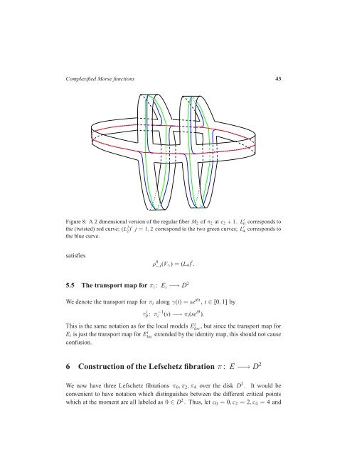
Complexified <strong>Morse</strong> <strong>functions</strong> 43<br />
Figure 8: A 2 dimensional version <strong>of</strong> the regular fiber M2 <strong>of</strong> π2 at c2 + 1. L ′ 0<br />
the (twisted) red curve; (L j<br />
2 )′ j = 1, 2 correspond to the two green curves; L ′ 4<br />
the blue curve.<br />
satisfies<br />
ρ 4 −s(Vγ) = (L4) ′ .<br />
5.5 <strong>The</strong> transport map for πi : Ei −→ D 2<br />
We denote the transport map for πi along γ(t) = se iθt , t ∈ [0, 1] by<br />
τ i θ : π−1 i (s) −→ πi(se iθ ).<br />
corresponds to<br />
corresponds to<br />
This is the same notation as for the local models Ei loc , but since the transport map for<br />
Ei is just the transport map for Ei loc extended by the identity map, this should not cause<br />
confusion.<br />
6 Construction <strong>of</strong> the <strong>Lefschetz</strong> fibration π : E −→ D 2<br />
We now have three <strong>Lefschetz</strong> fibrations π0,π2,π4 over the disk D 2 . It would be<br />
convenient to have notation which distinguishes between the different critical points<br />
which at the moment are all labeled as 0 ∈ D 2 . Thus, let c0 = 0, c2 = 2, c4 = 4 and


