The Picard-Lefschetz theory of complexified Morse functions 1 ...

Complexified Morse functions 65
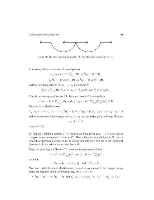
Figure 11: The four vanishing paths for (E, π) in the case when dim N = 3.
In summary, there are canonical isomorphisms
π −1
0 (c0 + 1) ∼ = T L1
−π/2 (M), π−1
1 (c1 + 1) ∼ = M,
π −1
2 (c2 + 1) ∼ = T L2
π/2 (M), π−1
3 (c3 − 1) ∼ = T L2
π/2 (M),
and the vanishing spheres for π0,...,π3 correspond to
L ′ 0 ⊂ T L1
−π/2 (M), L1 ⊂ M, L ′ 2 ⊂ T L2
π/2 (M), and L′ 3 ⊂ T L2
π/2 (M).
Now, by an analogue of lemma 6.1, there are canonical isomorphisms
π −1
1 (c1 − 1) ∼ = T L1
−π/2 (M), and π−1
2 (c2 + 1) ∼ = T L2
−π/2 (TL2 π/2 (M)) ∼ = M.
Thus we have identifications
π −1
0 (c0 + 1) ∼ = π −1
1 (c1 − 1),π −1
1 (c1 + 1) ∼ = π −1
2 (c2 − 1),π −1
2 (c2 + 1) ∼ = π −1
3 (c3 − 1)
and we use these to fiber connect sum π0,π1,π2,π3 (see §6) to get a Lefschetz fibration
where S ∼ = D 2 .
π : E −→ S
To find the vanishing spheres of π, choose the base point at c1 + 1/4 and choose
transport maps analogous to those in §7. That is they are straight lines in R, except
when they approach a critical value, in which case they do a half arc in the lower half
plane to avoid the critical value. See figure 11.
Then, by an analogue of lemma 7.2, there are symplectomorphisms
such that
τ1 : M −→ T L1
−π/2 (M), and τ2 : M −→ T L2
π/2 (M)
τ1(L0) = L ′ 0, τ2(L2) = L ′ 2, and τ2(L3) = L ′ 3.
Moreover, under the above identifications, τ1 and τ2 correspond to the transport maps
along the half arcs in the lower half plane, for 0 < s ≤ 1:
π −1
1 (c1 + s) −→ π −1
1 (c1 − s), and π −1
1 (c1 + s) ∼ = π −1
2 (c2 − s) −→ π −1
2 (c1 + s).