- Page 1 and 2:
Proceedings Eighth International Sy
- Page 3 and 4:
1987 by the American Society for Ph
- Page 5 and 6:
A NOTE ON THE FUTURE OF AUTO-CARTO
- Page 7 and 8:
Algorithms for spatial search or qu
- Page 9 and 10:
Research into electronic maps and a
- Page 11 and 12:
Sandhu, Jatinder 403 Shea, K. Stuar
- Page 13 and 14:
integration of the findings on tech
- Page 15 and 16:
departments of municipalities are p
- Page 17 and 18:
systems, similar cost reduction in
- Page 19 and 20:
exist here: it is rarely possible t
- Page 21 and 22:
REFERENCES Chris man, N. and Nieman
- Page 23 and 24:
THE USER PROFILE FOR DIGITAL CARTOG
- Page 25 and 26:
second is to reduce all lines to a
- Page 27 and 28:
OVERLAY PROCESSING IN SPATIAL INFOR
- Page 29 and 30:
digital terrain models, or magnetic
- Page 31 and 32:
(2-dimensional) or volumes (3-dimen
- Page 33 and 34: whereas the lattice induced by spat
- Page 35 and 36: 5.2 Overlay Operation One of the mo
- Page 37 and 38: permit the determination of the len
- Page 39 and 40: more about the quality of the avail
- Page 41 and 42: of the user interface and would res
- Page 43 and 44: FUNDAMENTAL PRINCIPLES OF GEOGRAPHI
- Page 45 and 46: of continuous space (the model of A
- Page 47 and 48: look like is transmitted through th
- Page 49 and 50: (Sullivan and others, 1985). On the
- Page 51 and 52: PRESCRIPTIONS To carry out the prin
- Page 53 and 54: AN ADAPTIVE METHODOLOGY FOR AUTOMAT
- Page 55 and 56: They reorganize available space and
- Page 57 and 58: Global Filtering Basics: This filte
- Page 59 and 60: If the geometry is determined throu
- Page 61 and 62: SYSTEMATIC SELECTION OF VERY IMPORT
- Page 63 and 64: Improvements The first improvement
- Page 65 and 66: RESULTS ANALYSIS There are two test
- Page 67 and 68: Figure 4. A TIN generated from VIP
- Page 69 and 70: only or the most important one. Unt
- Page 71 and 72: terrain surface, may have in corres
- Page 73 and 74: Advantages of determining the Media
- Page 75 and 76: egards points, only the endpoints o
- Page 77 and 78: contours some measures of size and
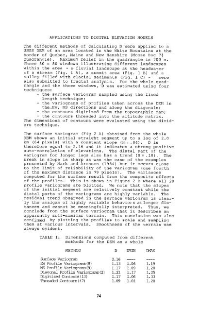
- Page 79 and 80: MEASURING THE DIMENSION OF SURFACES
- Page 81 and 82: dimension of an entity, is constant
- Page 83: terrain. In order to avoid a sampli
- Page 87 and 88: 1.20 1.16 • D I M 1.12 E N S 1.06
- Page 89 and 90: Stability of Map Topology and Robus
- Page 91 and 92: The 0-cells in the usual topologica
- Page 93 and 94: Notice in Figure 1 that the interme
- Page 95 and 96: Algorithm for computing robustness
- Page 97 and 98: We may sum the forces by a straight
- Page 99 and 100: and computational algorithms, which
- Page 101 and 102: The geopositioning model presented
- Page 103 and 104: It should be noted that only the fr
- Page 105 and 106: While Voronoi polygons have often b
- Page 107 and 108: additional vector rotation about th
- Page 109 and 110: inconsistency. The problem stems fr
- Page 111 and 112: Chain Intersection Determining chai
- Page 113 and 114: node(6,[h(l8),t(l9),t(24),h(21)]).
- Page 115 and 116: Sliver Removal. We remove a sliver
- Page 117 and 118: Little, J.J. and Peucker, T.K. 1979
- Page 119 and 120: measured control points. In this pa
- Page 121 and 122: TEST RESULTS For testing the above
- Page 123 and 124: A SPATIAL DECISION SUPPORT SYSTEM F
- Page 125 and 126: data by time period, by category, a
- Page 127 and 128: BASIC version of the PLACE suite re
- Page 129 and 130: procedural language. The classifier
- Page 131 and 132: FIGURE 1: SOFTWARE COMPONENTS FOR S
- Page 133 and 134: Realistic Flow Analysis Using a Sim
- Page 135 and 136:
Realistic Flow Analysis Using a Sim
- Page 137 and 138:
Realistic Flow Analysis Using a Sim
- Page 139 and 140:
Realistic Flow Analysis Using a Sim
- Page 141 and 142:
TIN FORMAT VS. MATRIX FORMAT The pr
- Page 143 and 144:
One of the major challenges involve
- Page 145 and 146:
Because TINFLOW is a PC-based GIS,
- Page 147 and 148:
Art; I DitH ot twin 1.1610 Strew He
- Page 149 and 150:
RATIONALE Gridded surface data sets
- Page 151 and 152:
5. For each polygon, for each cell
- Page 153 and 154:
A mapping function was used to topo
- Page 155 and 156:
CONCLUSIONS This depression-finding
- Page 157 and 158:
Methods For spatial analusis The tw
- Page 159 and 160:
1. Sampling to determine the sample
- Page 161 and 162:
A simcle multiscale model . Instead
- Page 163 and 164:
Complex multiscale models. The one-
- Page 165 and 166:
Mandelbrot, B.B., 198E. The Fractal
- Page 167 and 168:
A number of authors have proved the
- Page 169 and 170:
Once having the Fourier-transf arm
- Page 171 and 172:
From the above listed aspects (2) i
- Page 173 and 174:
A considerably large number of labo
- Page 175 and 176:
Oliver,M.A., R.Webster (1936) Semi-
- Page 177 and 178:
model can be used as the basis for
- Page 179 and 180:
ts phase space by analogy to phase
- Page 181 and 182:
Figure 3. Classified 64 by 64 raste
- Page 183 and 184:
in the delimitation of domains in p
- Page 185 and 186:
Mark, D.M. and Aronson, P.B. 1984,
- Page 187 and 188:
To make decisions about this world,
- Page 189 and 190:
Limitations inherent to the modeliz
- Page 191 and 192:
operations delimiting rights to the
- Page 193 and 194:
Uncertainty absorption is very diff
- Page 195 and 196:
Minsky, M. L. 1965, Matter, Minds,
- Page 197 and 198:
data, covering extremely large area
- Page 199 and 200:
Figure 1. a) Test data set with, tr
- Page 201 and 202:
Figure 2. Four pyramids - line segm
- Page 203 and 204:
convenient to consider grids to be
- Page 205 and 206:
REFERENCES Davis, J.C., 1973, Stati
- Page 207 and 208:
the data element, in this case an a
- Page 209 and 210:
EXPERIENCE WITH R-TREES IN A CIS LA
- Page 211 and 212:
REFERENCES Guttman, A. 1984, R-Tree
- Page 213 and 214:
World Shoreline Vectors Shoreline v
- Page 215 and 216:
Table 4. Applications of gridded el
- Page 217 and 218:
classes desired for a given applica
- Page 219 and 220:
Table 6. The impact of block size o
- Page 221 and 222:
Jones, Christopher B. and Abraham,
- Page 223 and 224:
DISADVANTAGES OF A SINGLE COVERAGE
- Page 225 and 226:
faster and less complex than genera
- Page 227 and 228:
NOS detailed source data 20 meter r
- Page 229 and 230:
si '- /W^ ?f ? ( " ( I?
- Page 231 and 232:
REFERENCES Aronson P. and Morehouse
- Page 233 and 234:
with the purpose of optimizing geom
- Page 235 and 236:
purposes, the value 1/e may be thou
- Page 237 and 238:
V describing points/ / y/ B / /•*
- Page 239 and 240:
clarity, the number of describing p
- Page 241 and 242:
ACKNOWLEDGMENTS The author wishes t
- Page 243 and 244:
INTRODUCTION In any application of
- Page 245 and 246:
7T 0 — 7T X Hay River Figure 1: A
- Page 247 and 248:
0 — 7T Alluvial fan contour Figur
- Page 249 and 250:
Peucker, 1973) can be used here; th
- Page 251 and 252:
Mark, D. M., 1985, Fundamental spat
- Page 253 and 254:
•©—e—©—e- Figure 1.1: Spl
- Page 255 and 256:
SLAU- 9/1000 Figure 1.5: Results of
- Page 257 and 258:
t-0 I.I 7.4 /.6 1.8 2.0 Figure 2.1:
- Page 260 and 261:
THE TIGER STRUCTURE Christine Kinne
- Page 262 and 263:
to another tail record. There are f
- Page 264 and 265:
Since records are fixed length, a n
- Page 266 and 267:
areal data is stored, but additiona
- Page 268 and 269:
KEY TO SUBFILE ABBREVIATIONS (CONTI
- Page 270 and 271:
TOPOLOGICAL ENTITIES Corbett's topo
- Page 272 and 273:
TOPOLOGICAL RULES The preceding def
- Page 274 and 275:
File and the new linear feature ref
- Page 276 and 277:
Encoding and Referencing (TIGER) Sy
- Page 278 and 279:
of the boundary are found and corre
- Page 280 and 281:
CONCLUSION The GTUB routines have b
- Page 282 and 283:
SELECTION OF EQUIPMENT The least ef
- Page 284 and 285:
operations. The site and staff for
- Page 286 and 287:
RESULTS Table one shows the numeric
- Page 288 and 289:
would no longer have to determine a
- Page 290 and 291:
THE DATA BASE ADVANTAGE Most of the
- Page 292 and 293:
SUMMARY AND CONCLUSIONS The major d
- Page 294 and 295:
the complexity o-f I/O processing.
- Page 296 and 297:
is on one and only one topological
- Page 298 and 299:
•features represented in the data
- Page 300 and 301:
intersection is -found -for this -f
- Page 302 and 303:
An easy implementation o-f spatial
- Page 304 and 305:
organisations most precious asset -
- Page 306 and 307:
no reason why we should not model t
- Page 308 and 309:
- A VERTEX identifies a unique spat
- Page 310 and 311:
to the organisation and indexing of
- Page 312 and 313:
the retrieval of data from the disp
- Page 314 and 315:
original goals, through design, and
- Page 316 and 317:
Contents and Queries Each geographi
- Page 318 and 319:
number of tables required. On the o
- Page 320 and 321:
generic, db-internal read/write/del
- Page 322 and 323:
we are guaranteed that each occurre
- Page 324 and 325:
The db bottlenecks we found were, f
- Page 326 and 327:
Bibliography [1] Date, C.J. 1983 -
- Page 328 and 329:
model is an object-oriented extensi
- Page 330 and 331:
SPECIALIZATIONS FOR SPATIAL DATA Th
- Page 332 and 333:
for each x in S, for each y in S if
- Page 334 and 335:
entity IMAGE PIXELS(IMAGE) - set of
- Page 336 and 337:
Orenstem, J.A. 1984, "A Class of Da
- Page 338 and 339:
understand the data model on which
- Page 340 and 341:
Internally, KGIS is implemented on
- Page 342 and 343:
AREA > 10; Spatial relationships be
- Page 344 and 345:
Once established, a GEOVIEW remains
- Page 346 and 347:
___________, 1985, THE USE OF SPATI
- Page 348 and 349:
• the cross sections, profiles an
- Page 350 and 351:
• Rigid and homogeneous ores can
- Page 352 and 353:
Borehole data \ Geologist's ^^ know
- Page 354 and 355:
Figure 3 : A Portion of the Ore Bod
- Page 356 and 357:
REFERENCES Baumgart, E.G. (1975) -
- Page 358 and 359:
This paper is organized into five s
- Page 360 and 361:
yields the resulting table: Poly* 1
- Page 362 and 363:
tightly bound to the map; there is
- Page 364 and 365:
A partial example of the relational
- Page 366 and 367:
REFERENCES Chrisman N. and Niemann,
- Page 368 and 369:
GEOGRAPHIC DATABASE TOPOLOGY SPATIA
- Page 370 and 371:
of a coordinate in n-space, usually
- Page 372 and 373:
Airport refines Aviation; — This
- Page 374 and 375:
THE dbmap SYSTEM Donald F. Cooke Ge
- Page 376 and 377:
procedurally, like Pascal, FORTRAN
- Page 378 and 379:
een lassoed (and line-segments in o
- Page 380 and 381:
Figure 4 Result of Lasso Operation
- Page 382 and 383:
The goal of a DSS is to help decisi
- Page 384 and 385:
chosen structure must provide a mea
- Page 386 and 387:
First, a general schema diagram is
- Page 388 and 389:
Hopkins, L.D., and Armstrong, M.P.
- Page 390 and 391:
******* DATABASE IDENTIFICATION AND
- Page 392 and 393:
Because of these limitations, furth
- Page 394 and 395:
cannot share the data. A minicomput
- Page 396 and 397:
Historically the whole orientation
- Page 398 and 399:
To reach the stated goal of this pa
- Page 400 and 401:
mapping techniques conceptualized a
- Page 402 and 403:
The future skill level, and trainin
- Page 404 and 405:
€6€ COMPUTER SCIENTIST ELECTRIC
- Page 406 and 407:
U* '^ OUTPUT \ / REVIEWIM. CORRECTI
- Page 408 and 409:
We may conceptually divide a VNA in
- Page 410 and 411:
most interest for transmitting navi
- Page 412 and 413:
necessary) in such a display. This
- Page 414 and 415:
ENHANCEMENT AND TESTING OF A MICROC
- Page 416 and 417:
make maximum use of the limited, lo
- Page 418 and 419:
I Text Display Window (Toggle On/Of
- Page 420 and 421:
as well, using the PLINK86 Plus ove
- Page 422 and 423:
AN INTEGRATED PC BASED CIS FOR INST
- Page 424 and 425:
RAW DATA INPUT DATA BASE MAPh ANALY
- Page 426 and 427:
Figure 3. Example of output from SH
- Page 428 and 429:
Figure 8. CONTOUR of elevation on v
- Page 430 and 431:
Figure 11. COLOR map on printer of
- Page 432 and 433:
IDRISI : A COLLECTIVE GEOGRAPHIC AN
- Page 434 and 435:
felt to be negligible compared to t
- Page 436 and 437:
Although the IDRISI system was prim
- Page 438 and 439:
data file, and a second backwards t
- Page 440 and 441:
TABLE 1 : IDRISI PROGRAM MODULES IN
- Page 442 and 443:
CLASSLESS CHOROPLETH MAPPING WITH M
- Page 444 and 445:
polygon. The process of selecting s
- Page 446 and 447:
There are a number of places where
- Page 448 and 449:
COMPUTER-ASSISTED TERRAIN ANALYSIS
- Page 450 and 451:
2. Input. A digitizing tablet to al
- Page 452 and 453:
terrain analysis data. Items 3. and
- Page 454 and 455:
Database Structure Currently, DMA-p
- Page 456 and 457:
RESULTS OF THE DANE COUNTY LAND REC
- Page 458 and 459:
E. G.
- Page 460 and 461:
section maps of tax parcels maintai
- Page 462 and 463:
Public Land Survey System (PLSS) co
- Page 464 and 465:
Sheets, Proc. ACSM, 1:153-161. Chri
- Page 466 and 467:
von Meyer, N.R. 1984b. Westport Ine
- Page 468 and 469:
While meeting the above criteria pr
- Page 470 and 471:
oundary line. An example of the sam
- Page 472 and 473:
Four groups of approximately thirty
- Page 474 and 475:
LEGEND MULTIPLE BOUNDARIES STATE, C
- Page 476 and 477:
TABLE 2 shows that more respondents
- Page 478 and 479:
What features are considered when d
- Page 480 and 481:
position is insignificant. Thus, th
- Page 482 and 483:
ASSESSING COMMUNITY VULNERABILITY T
- Page 484 and 485:
Yale University was selected for st
- Page 486 and 487:
distribution of hazardous materials
- Page 488 and 489:
»++ 0000000001000OCCCOOOOOOCOOOOCO
- Page 490 and 491:
44* 444 444 ICO 9 CO 9CO to CO ECO
- Page 492 and 493:
IMPROVEMENT OF GBF/DIME FILE COORDI
- Page 494 and 495:
Establishment of Control Points In
- Page 496 and 497:
transformation parameters for a par
- Page 498 and 499:
of using a fixed set of transformat
- Page 500 and 501:
vertex coordinates into exact corre
- Page 502 and 503:
Friedman, J., Baskett, F. and Shust
- Page 504 and 505:
and small freehold land. It does no
- Page 506 and 507:
The next step in the planning proce
- Page 508 and 509:
TSO on UNB's IBM 3090 mainframe com
- Page 510 and 511:
3. Kettela, E.G. 1975. Aerial spray
- Page 512 and 513:
The integration of developing techn
- Page 514 and 515:
and photographic processes are used
- Page 516 and 517:
Figure 4 EXAMPLE OF PUBLISHED FIRM
- Page 518 and 519:
EXAMPLE OF COMPUTER-GENERATED FIRM
- Page 520 and 521:
BIBLIOGRAPHY Federal Emergency Mana
- Page 522 and 523:
more detailed introduction to exper
- Page 524 and 525:
MAPEX is a rule-based system for au
- Page 526 and 527:
discrimination nets, Click et al (1
- Page 528 and 529:
example, FES (Goldberg et al, 1984.
- Page 530 and 531:
Pereira, L.M., P. Sabatier, and E.
- Page 532 and 533:
e flexible enough to address a wide
- Page 534 and 535:
intermediate hypotheses are "posted
- Page 536 and 537:
All cited rules become part of the
- Page 538 and 539:
The Geographic Information System L
- Page 540 and 541:
geographic knowledge system applies
- Page 542 and 543:
In view of this it is not suprising
- Page 544 and 545:
placement, the main area of cartogr
- Page 546 and 547:
EXPERT SYSTEM INTERFACE TO A GEOGRA
- Page 548 and 549:
ASPENEX automates the analysis of s
- Page 550 and 551:
Rule-Base Creation SYSTEM OPERATION
- Page 552 and 553:
the rulebase created by the aspen e
- Page 554 and 555:
AUTOMOBILE NAVIGATION IN THE PAST E
- Page 556 and 557:
oadside equipment to provide equipp
- Page 558 and 559:
algorithm and provides step-by-step
- Page 560 and 561:
DRIVER INPUTS • DESTINA1ION • R
- Page 562 and 563:
Vehicular Technology Conference, 35
- Page 564 and 565:
Map retrieval is also crucial to na
- Page 566 and 567:
elative coordinate accuracy is very
- Page 568 and 569:
destination does not require knowin
- Page 570 and 571:
PRESENTATION The extremes of styles
- Page 572 and 573:
REFERENCES Ashkenazi, V. 1986, Coor
- Page 574 and 575:
decision-making, learning, and natu
- Page 576 and 577:
that these travellers felt that wri
- Page 578 and 579:
e weak, if present at all. Since ma
- Page 580 and 581:
Figure 2: An example of a distorted
- Page 582 and 583:
directions were produced in real ti
- Page 584 and 585:
Figure 1. Concept of an Automatic V
- Page 586 and 587:
AVL COMPONENTS AND THEIR FUNCTIONS
- Page 588 and 589:
OUTPUT FACILITIES V7MIC1Z «IflT KA
- Page 590 and 591:
need extensive customizing. This cu
- Page 592 and 593:
PRACTICAL EXPERIENCE WITH AVL 2000
- Page 594 and 595:
ACKNOWLEDGEMENT This research has b
- Page 596 and 597:
separate AVL system is needed (spec
- Page 598 and 599:
Sources Two plausible sources of a
- Page 600 and 601:
o t=z ATTRIBUTE RELATIONSHIP ENTITY
- Page 602 and 603:
(a) optimal route between the pair
- Page 604 and 605:
REFERENCES Cooke, D.F., Vehicle Nav
- Page 606 and 607:
THE BBC DOMESDAY SYSTEM: A NATION-W
- Page 608 and 609:
which are not commonplace: it permi
- Page 610 and 611:
Geochenrstrj Climate VNater fiature
- Page 612 and 613:
(ii) measure area and distance in m
- Page 614 and 615:
Rhind D.W. and Mounsey H.M. (1986).
- Page 616 and 617:
language expression. One of the mot
- Page 618 and 619:
This process begins from a position
- Page 620 and 621:
E(l(k)) be the expectation of I ( k
- Page 622 and 623:
There are several approaches to con
- Page 624 and 625:
In this paper we will discuss preml
- Page 626 and 627:
Table 2. Length of Sessions and The
- Page 628 and 629:
Table 5. Fuzzy Membership Values fo
- Page 630 and 631:
Table 7. Results of Zimraermann's M
- Page 632 and 633:
Chamberlain, D.D. and R.F. Boyce. 1
- Page 634 and 635:
ACCESSING LARGE SPATIAL DATA BASES
- Page 636 and 637:
WORKSTATION #2 1 - IBM-AT; 640K, 20
- Page 638 and 639:
RECORD 1 —— coordinates 1-256 f
- Page 640 and 641:
Future developments include the pol
- Page 642 and 643:
Once features of two coverages have
- Page 644 and 645:
Figure 3a Partial street network co
- Page 646 and 647:
Figure 3e Coverages aligned with 50
- Page 648 and 649:
Solving the Feature Matching Proble
- Page 650 and 651:
References Chen, Z. and A. Guevara,
- Page 652 and 653:
determined that a conversion of dra
- Page 654 and 655:
PAT GRP NUM 1 2 3 4 5 6 7 8 9 10 11
- Page 656 and 657:
various raster and vector operation
- Page 658 and 659:
Figure 4a - Portion of scan-digitiz
- Page 660 and 661:
the set of points. This will introd
- Page 662 and 663:
which represents the terrain by a t
- Page 664 and 665:
leaf for 4 and 5). Chen and Tobler
- Page 666 and 667:
fixed polynomial order for each run
- Page 668 and 669:
RESULTS As noted above, the program
- Page 670 and 671:
REFERENCES Chen, Z.-T., and Tobler,
- Page 672 and 673:
Shortcomings in Existing Raster-to-
- Page 674 and 675:
Template design parameters are base
- Page 676 and 677:
RESULTS REPORT type RESULTS REPORT
- Page 678 and 679:
Significance of the AFT Technology
- Page 680 and 681:
REFERENCES Antell, R.E. (1983), "Th
- Page 682 and 683:
Grid systems do not permit vertical
- Page 684 and 685:
SCHEMA structures an urban model ar
- Page 686 and 687:
The second data structure regards t
- Page 688 and 689:
The resulting polygon "hole" is the
- Page 690 and 691:
REFERENCES Brassel, Kurt E., and Do
- Page 692 and 693:
The link between these two bodies o
- Page 694 and 695:
The same technique of Fourier analy
- Page 696 and 697:
The similarities between this and t
- Page 698 and 699:
In many respects, a terrain model c
- Page 700 and 701:
AN ALGORITHM FOR LOCATING , CANDIDA
- Page 702 and 703:
The left and right boundaries of a
- Page 704 and 705:
limits. The overall problem of gene
- Page 706 and 707:
To find the cluster limits, the sim
- Page 708 and 709:
next box. The entry (m = s) is ther
- Page 710 and 711:
Figure 3.-Portion of test data set
- Page 712 and 713:
PRACTICAL EXPERIENCE WITH A MAP LAB
- Page 714 and 715:
£ X lfk = 1 k=1,2,...,K. (1) i If
- Page 716 and 717:
Deleted Labels The optimization alg
- Page 718 and 719:
Figure 2. Point Symbol Labels With
- Page 720 and 721:
AUTOMATIC RECOGNITION AND RESOLUTIO
- Page 722 and 723:
FUNCTION REQUIRED l)ls a point on a
- Page 724 and 725:
distance by finding the square root
- Page 726 and 727:
Proportional Radial Enlargement As
- Page 728 and 729:
distribution). If the thresholds ar
- Page 730 and 731:
CALCULATING BISECTOR SKELETONS USIN
- Page 732 and 733:
Thiessen centroid than to any other
- Page 734 and 735:
there are exactlv n boundary skelet
- Page 736 and 737:
AREA MATCHING IN RASTER MODE UPDATI
- Page 738 and 739:
THE AREA MATCHING PROCESS This proc
- Page 740 and 741:
defaults are made of very short seg
- Page 742 and 743:
POLYGONIZATION AND TOPOLOGICAL EDIT
- Page 744 and 745:
If no label exists between the chai
- Page 746 and 747:
these internal (non-boundary) chain
- Page 748 and 749:
However, a cartographic database ne
- Page 750 and 751:
"WYSIWYG" MAP DIGITIZING: REAL TIME
- Page 752 and 753:
with tolerance circles such that it
- Page 754 and 755:
CONCLUSION For many years a major i
- Page 756 and 757:
implementation methodology and the
- Page 758 and 759:
SPLIT SCREEN o o oo SIDE BY SIDE o
- Page 760 and 761:
determined applicability aided by s
- Page 762 and 763:
the 384 LPI resolution patch used t
- Page 764 and 765:
TESTING A PROTOTYPE SPATIAL DATA EX
- Page 766 and 767:
2. An Overview of MAPS The MAPS spa
- Page 768 and 769:
containment tree can be used to eff
- Page 770 and 771:
ROLE: BUILDING UNKNOWN MEDICAL CENT
- Page 772 and 773:
and the segment direction within ea
- Page 774:
seg : nodes: points south west: 20.