Investigation of the optically stimulated luminescence dating method ...
Investigation of the optically stimulated luminescence dating method ...
Investigation of the optically stimulated luminescence dating method ...

You also want an ePaper? Increase the reach of your titles
YUMPU automatically turns print PDFs into web optimized ePapers that Google loves.
Department <strong>of</strong> Analytical Chemistry<br />
Institute for Nuclear Sciences<br />
INVESTIGATION OF THE<br />
OPTICALLY STIMULATED LUMINESCENCE DATING METHOD<br />
FOR APPLICATION TO YOUNG GEOLOGICAL SEDIMENTS<br />
Dimitri Vandenberghe<br />
Thesis submitted in fulfilment <strong>of</strong> <strong>the</strong> requirements for <strong>the</strong> degree <strong>of</strong><br />
Doctor (PhD) <strong>of</strong> Science: Chemistry<br />
Promoter: Dr. F. De Corte<br />
Co-promoter: Pr<strong>of</strong>. Dr. P. Van den haute<br />
Academic year: 2003-2004
DANKWOORD<br />
Dr. F. De Corte dank ik voor de kans die hij mij heeft gegeven dit doctoraat te starten, en om de taak van<br />
promotor op zich te nemen. De manier waarop hij mij vertrouwd maakte met het nucleair-analytisch onderzoek,<br />
zonder hierbij de wetenschap nog moeilijker te maken dan ze al is, kon ik enorm waarderen. Dit doctoraatswerk<br />
is het allerlaatste proefschrift waarin de k0-<strong>method</strong>e werd toegepast, gebruik makend van reactor Thetis.<br />
Bovendien was ik waarschijnlijk ook de laatste doctoraatsstudent die Frans onder zijn konijnenvleugeltjes nam.<br />
Ik heb dan ook mijn uiterste best gedaan om van deze <strong>the</strong>sis iets te maken waar hij terecht trots kan op zijn.<br />
Ik wil Frans vooral bedanken voor het vertrouwen dat hij mij schonk en voor zijn onvoorwaardelijke steun,<br />
zowel pr<strong>of</strong>essioneel als daarbuiten.<br />
Ik dank Pr<strong>of</strong> Dr. P. Van den haute om de taak van co-promotor op zich te nemen en voor de ondersteuning bij<br />
het veldwerk. Verder dank ik hem voor de vele interessante toelichtingen bij de geologie en geochronologie, en<br />
voor de interessante wetenschappelijke discussies.<br />
Pr<strong>of</strong> Dr. Em. R. Dams en Pr<strong>of</strong> Dr. K. Strijckmans wens ik te bedanken voor het ter beschikking stellen van de<br />
infrastructuur.<br />
Dr. C. Kasse (Vrije Universiteit, Amsterdam) wil ik in het algemeen bedanken voor de productieve<br />
samenwerking. Meer in het bijzonder dank ik hem voor zijn hulp bij de keuze van de bemonsteringslocaties en<br />
bij het veldwerk. Zonder zijn bijdrage had ik het geologisch aspect van dit onderzoek niet zo stevig kunnen<br />
onderbouwen.<br />
I would like to thank Pr<strong>of</strong>. Dr. A.S. Murray (<strong>the</strong> Nordic Laboratory for Luminescence Dating) for his support<br />
throughout this entire work. I am very grateful for his willingness to participate in <strong>the</strong> interlaboratory<br />
comparison, for <strong>the</strong> stimulating discussions, and for sharing thoughts and Duvel...<br />
I also wish to thank Dr. M. Fuchs (Universität Bayreuth) for participating in <strong>the</strong> laboratory intercomparison and<br />
for providing samples. I really enjoyed our discussions, scientific or o<strong>the</strong>rwise, even more so as <strong>the</strong>se were <strong>of</strong>ten<br />
accompanied by a few beers.<br />
Grateful acknowledgement is made to Pr<strong>of</strong>. Dr. G. Wagner and co-workers at <strong>the</strong> Max Planck Institut for <strong>the</strong><br />
cordial manner by which <strong>the</strong>y have received us in Heidelberg. I wish to thank especially Dr. A. Kadereit en Dr.<br />
R. Kalchgruber for <strong>the</strong> valuable discussions, and for providing samples and literature.<br />
More in general, I would like to express my gratitude to all members <strong>of</strong> <strong>the</strong> German <strong>luminescence</strong> <strong>dating</strong><br />
community, for having me at <strong>the</strong>ir meetings and for <strong>the</strong> warm manner by which <strong>the</strong>y welcomed me <strong>the</strong>re. I thank<br />
<strong>the</strong>m for <strong>the</strong> many useful discussions and suggestions, and for <strong>the</strong> great time before, in between and after<br />
scientific sessions.<br />
I thank Till Fink for sending a copy <strong>of</strong> his <strong>the</strong>sis and for <strong>the</strong> unforgettable time in Marburg.<br />
Grateful acknowledgement is made to Dr. L. Bøtter-Jensen and his co-workers (Risø National Laboratory) for<br />
allowing me to visit <strong>the</strong>ir lab. I wish to express my sincere thanks to Henrik Christiansen for providing technical<br />
support and for answering all <strong>the</strong> questions I had regarding <strong>the</strong> OSL-measurement apparatus.<br />
I thank Dr. J.M. Olley for <strong>the</strong> “Radial plot” program, and Pr<strong>of</strong>. Dr. D.J. Huntley for <strong>the</strong> Dose-Intercept program.<br />
I am grateful to Dr. M.D. Bateman for allowing me access to his unpublished data <strong>of</strong> <strong>the</strong> Grubbenvorst sands.
I would also like to thank <strong>the</strong> many <strong>luminescence</strong> workers around <strong>the</strong> world that shared ideas with me, provided<br />
me with reading material, and bo<strong>the</strong>red to reply to my sometimes time-consuming questionnaires.<br />
Alle collega-doctorandi dank ik voor de aangename werksfeer op het INW; in het bijzonder Jan en Marijn voor<br />
de leuke gesprekken en voor het blijven hangen op recepties en feestjes. I am grateful to S.M. Hossain, who was<br />
my nearest colleague for about four years. His kind and warm companionship made <strong>the</strong> long hours at <strong>the</strong> <strong>of</strong>fice<br />
much more agreeable. His work on <strong>the</strong> determination <strong>of</strong> <strong>the</strong> annual dose-rate was essential for <strong>the</strong> preparation <strong>of</strong><br />
this <strong>the</strong>sis.<br />
Collega-doctorandus Jan-Pieter wil ik bedanken voor de interessante gesprekken en de hulp bij verschillende<br />
geologisch facetten van het onderzoek, voor de vriendschap na de werkuren en zijn liefde voor de tripel.<br />
Caroline, Mathieu en Herman wens ik te bedanken voor de indirecte bijdrage die ze met hun Licentiaats<strong>the</strong>sis<br />
aan dit werk hebben geleverd, en voor hun aangenaam gezelschap.<br />
Zonder de nauwgezette hulp van Jochem bij nagenoeg alle praktische aspecten van dit onderzoek, was dit werk<br />
zowel kwalitatief als kwantitatief heel wat minder uitgebreid geweest. Ik ben hem vooral zeer dankbaar voor zijn<br />
onvoorwaardelijke vriendschap.<br />
Ing. A. “Tony” De Wispelaere dank ik voor zijn bereidwillige, efficiënte en vriendelijke hulp bij de bestralingen<br />
en bij allerhande meet- en rekenwerk.<br />
Alle administatrieve en technische personeelsleden hebben op de één <strong>of</strong> andere manier bijgedragen tot de<br />
totstandkoming van dit werk. Ze zorgden ook voor pret en (veel…) verzet. Ik wil Marc bedanken voor het<br />
maken van verschillende monsterhouders en voor het boren van de vele (soms te veel…) gaten, en Maurice voor<br />
het blazen van de flotatiecel (een waarachtig artisanaal kunstwerk). Chantal was onmisbaar bij de administratie<br />
en ik ben haar ook dankbaar voor de babbels. Lucien dank ik voor het soigneren van Berta en Amanda, voor de<br />
occasionele pint en voor de reddende plukjes tabak. Jacques, Rudy en Jos dank ik voor de hulp bij de<br />
bestralingen. Zonder Rudy waren bovendien ook mijn weerstanden waarschijnlijk meer dan eens gesmolten, en<br />
ik dank hem voor zijn snelle bijstand. Jos wens ik te bedanken voor zijn hulp bij allerlei s<strong>of</strong>tware problemen, en<br />
vooral om mij op tijd uit de illegaliteit van het downloaden te redden. Alhoewel reeds een aantal jaren niet meer<br />
op het INW werkzaam, dank ik Ruth voor de overlevering van haar praktische kennis met betrekking tot de<br />
monstervoorbereiding, haar aangenaam gezelschap in de donkere kamer en tijdens het studieverblijf in Risø. Jan,<br />
Johan en Roger dank ik voor de aangename keuvels. Hugo Palmans wens ik te bedanken voor het uitvoeren van<br />
de gamma bestralingen.<br />
Tot slot wens ik mijn familie te bedanken, in het bijzonder Barbara, mama en E<strong>the</strong>l. Zonder hun liefde en<br />
constante steun, hun begrip voor de vele overuren, en hun eindeloos geduld met mijn luimen, was dit werk nooit<br />
voltooid.<br />
Dit onderzoek kwam tot stand met de financiële steun van het Fonds voor Wetenschappelijk Onderzoek, het<br />
Bijzonder Onderzoeksfonds van de Universiteit Gent, en Wilfried Hoste.
CONTENTS<br />
Introduction.........................................................................................................................1<br />
Chapter 1: Essentials <strong>of</strong> <strong>luminescence</strong> <strong>dating</strong> ..................................................................5<br />
1.1. General principles <strong>of</strong> <strong>luminescence</strong> <strong>dating</strong> ....................................................5<br />
1.2. Mechanism .....................................................................................................7<br />
1.3. Signal growth and trap stability .....................................................................9<br />
1.4. Anomalous fading ........................................................................................13<br />
1.5. Stimulation <strong>of</strong> <strong>the</strong> signal ..............................................................................14<br />
1.6. Minerals used for optical <strong>dating</strong>...................................................................16<br />
Chapter 2: OSL from quartz ...........................................................................................17<br />
2.1. Stimulation <strong>of</strong> quartz....................................................................................17<br />
2.2. Emission by quartz.......................................................................................19<br />
2.3. Measuring <strong>the</strong> OSL from quartz...................................................................21<br />
2.4. The quartz shine-down curve .......................................................................22<br />
2.5. Quartz OSL components ..............................................................................30<br />
2.6. Signal stability..............................................................................................32<br />
2.7. Sensitivity changes.......................................................................................34<br />
2.8. Intrinsic <strong>luminescence</strong> characteristics..........................................................38<br />
2.8.1. Specific <strong>luminescence</strong>.......................................................................38<br />
2.8.2. Components ......................................................................................40<br />
2.8.3. Signal growth ....................................................................................41<br />
2.9. Resetting <strong>of</strong> <strong>the</strong> quartz OSL signal ..............................................................42<br />
2.10. The relationship between OSL and TL <strong>of</strong> quartz.........................................47<br />
Chapter 3: The optical <strong>dating</strong> <strong>method</strong> ............................................................................51<br />
3.1. The age equation ..........................................................................................51<br />
3.2. The equivalent dose......................................................................................52<br />
3.2.1. Techniques for equivalent dose determination .................................52<br />
3.2.1.1. Multiple-aliquot techniques .............................................52<br />
3.2.1.1.1. The multiple-aliquot additive-dose technique<br />
(MAAD) ...............................................................53<br />
3.2.1.1.2. The multiple-aliquot regenerative-dose technique<br />
(MARD)................................................................54<br />
3.2.1.1.3. The “Australian slide” technique..........................55<br />
3.2.1.1.4. The single-aliquot regeneration and added-dose<br />
technique (SARA) ................................................57<br />
3.2.1.2. Single-aliquot techniques.................................................61<br />
3.2.1.2.1. The single-aliquot additive-dose technique<br />
(SAAD).................................................................61
II Contents<br />
3.2.1.2.2. The single-aliquot regenerative-dose technique<br />
(SAR)....................................................................64<br />
3.2.2. Preheating and <strong>the</strong>rmal transfer ........................................................75<br />
3.2.2.1. Preheating ........................................................................75<br />
3.2.2.2. Unwanted <strong>the</strong>rmal transfer...............................................79<br />
3.2.3. Equivalent dose variability ...............................................................82<br />
3.2.3.1. Partial bleaching...............................................................83<br />
3.2.3.2. Microdosimetry................................................................86<br />
3.2.3.3. Post-depositional mixing .................................................87<br />
3.2.3.4. Analysis <strong>of</strong> equivalent dose variability............................88<br />
3.2.3.4.1. Dose distribution <strong>method</strong>s....................................89<br />
3.2.3.4.2. Signal analysis <strong>method</strong>s........................................95<br />
3.3. The annual dose............................................................................................99<br />
3.3.1. Natural radioactivity .........................................................................99<br />
3.3.2. Radioactive disequilibria ................................................................102<br />
3.3.3. Cosmic radiation .............................................................................104<br />
3.3.4. Techniques for annual dose determination .....................................106<br />
3.3.5. The effect <strong>of</strong> moisture.....................................................................107<br />
3.3.6. Efficiency........................................................................................108<br />
3.3.7. Attenuation and <strong>the</strong> effect <strong>of</strong> etching..............................................109<br />
3.3.8. The contribution <strong>of</strong> 87 Rb .................................................................115<br />
3.3.9. Internal radioactivity.......................................................................116<br />
Chapter 4: Implementation <strong>of</strong> <strong>the</strong> optical <strong>dating</strong> <strong>method</strong> – a pilot study on <strong>the</strong><br />
coversands from Ossendrecht ........................................................................................119<br />
4.1. Introduction ................................................................................................119<br />
4.2. Geological setting.......................................................................................119<br />
4.3. Independent age information......................................................................124<br />
4.4. Sampling and field measurements..............................................................127<br />
4.5. Equivalent dose determination...................................................................129<br />
4.5.1. Sample preparation .........................................................................129<br />
4.5.2. Aliquot preparation and presentation..............................................132<br />
4.5.3. Sample purity ..................................................................................133<br />
4.5.4. Measurement and irradiation facilities............................................135<br />
4.5.5. Data collection and processing .......................................................139<br />
4.5.6. Calibration <strong>of</strong> <strong>the</strong> irradiation facilities............................................140<br />
4.5.7. Equivalent dose determination........................................................143<br />
4.5.7.1. De determination using <strong>the</strong> multiple-aliquot additive-dose<br />
(MAAD) technique ........................................................143<br />
4.5.7.2. De determination using <strong>the</strong> single-aliquot additive-dose<br />
(SAAD) technique .........................................................144<br />
4.5.7.3. De determination using <strong>the</strong> single-aliquot regenerativedose<br />
(SAR) technique ....................................................147<br />
4.5.7.4. evaluation <strong>of</strong> <strong>the</strong> MAAD and SAR technique ...............156<br />
4.6. Annual dose determination.........................................................................158<br />
4.6.1. Gamma-ray spectrometry................................................................159
Contents III<br />
4.6.1.1. Field NaI(Tl) gamma-ray spectrometry.........................159<br />
4.6.1.2. Low-background Ge gamma-ray spectrometry .............160<br />
4.6.2. Neutron activation analysis.............................................................164<br />
4.6.3. Thick source alpha counting ...........................................................167<br />
4.6.4. Evaluation <strong>of</strong> <strong>the</strong> results..................................................................168<br />
4.6.5. Conversion factors ..........................................................................173<br />
4.7. Age calculation, optical ages and discussion .............................................174<br />
4.8. Fur<strong>the</strong>r equivalent dose determination using SAR ....................................179<br />
4.8.1. Determination <strong>of</strong> <strong>the</strong> De distributions .............................................180<br />
4.8.2. <strong>Investigation</strong>s on <strong>the</strong> origin <strong>of</strong> <strong>the</strong> dose distributions .....................183<br />
4.8.2.1. Experimental artefact? ...................................................183<br />
4.8.2.2. Partial bleaching?...........................................................185<br />
4.8.2.3. Variations in microdosimetry?.......................................189<br />
4.8.3. Discussion .......................................................................................191<br />
4.9. Conclusions ................................................................................................192<br />
Chapter 5: Application <strong>of</strong> <strong>the</strong> optical <strong>dating</strong> <strong>method</strong> in a case-study – <strong>the</strong> Late<br />
Pleniglacial coversands <strong>of</strong> Grubbenvorst ....................................................................195<br />
5.1. Introduction ................................................................................................195<br />
5.2. Geological setting.......................................................................................195<br />
5.3. Independent age information......................................................................199<br />
5.4. Sampling and field measurements..............................................................202<br />
5.5. Equivalent dose determination...................................................................208<br />
5.5.1. Sample preparation .........................................................................208<br />
5.5.2. Aliquot preparation and presentation..............................................208<br />
5.5.3. Equivalent dose determination........................................................209<br />
5.5.3.1. Influence <strong>of</strong> <strong>the</strong> preheat temperature on <strong>the</strong> De .............209<br />
5.5.3.2. Influence <strong>of</strong> <strong>the</strong> size <strong>of</strong> <strong>the</strong> test dose on <strong>the</strong> De..............217<br />
5.5.3.3. Dose recovery tests ........................................................219<br />
5.5.3.4. Equivalent dose distributions.........................................226<br />
5.5.3.4.1. Dose distribution in <strong>the</strong> aeolian sample (G9) .....226<br />
5.5.3.4.2. Dose distributions in <strong>the</strong> fluvio-aeolian samples<br />
(G1, G7 and G8) .................................................231<br />
5.5.3.4.3. Dose distributions in <strong>the</strong> fluvio-aeolian / fluvial<br />
samples (G3 and G4) ..........................................235<br />
5.5.3.4.4. Dose distributions in <strong>the</strong> fluvial samples (G10 and<br />
G21) ...................................................................238<br />
5.5.3.4.5. Discussion...........................................................241<br />
5.6. Annual dose determination.........................................................................244<br />
5.6.1. Gamma-ray spectrometry................................................................244<br />
5.6.1.1. Field NaI(Tl) gamma-ray spectrometry.........................244<br />
5.6.1.2. Low-background Ge gamma-ray spectrometry .............245<br />
5.6.2. Neutron activation analysis.............................................................253<br />
5.6.3. Thick source alpha counting ...........................................................255<br />
5.6.4. Comparison and evaluation <strong>of</strong> <strong>the</strong> results.......................................259
IV Contents<br />
5.6.4.1. Comparison <strong>of</strong> field with low-level gamma-ray<br />
spectrometry...................................................................259<br />
5.6.4.2. Comparison <strong>of</strong> k0-NAA with low-level gamma-ray<br />
spectrometry...................................................................260<br />
5.6.4.3. Comparison <strong>of</strong> observed with predicted alpha<br />
count-rates......................................................................264<br />
5.7. Age calculation, optical ages and discussion .............................................267<br />
5.8. Conclusions ................................................................................................274<br />
Summary and conclusions..............................................................................................275<br />
Appendix: A note on pairs counting..............................................................................280<br />
Nederlandse samenvatting .............................................................................................291<br />
References
INTRODUCTION<br />
The exact reconstruction <strong>of</strong> past events and processes plays a very important role in a<br />
number <strong>of</strong> scientific disciplines, such as geology and archaeology. An accurate and<br />
precise knowledge <strong>of</strong> <strong>the</strong> time when certain events took place, <strong>of</strong> <strong>the</strong> duration <strong>of</strong> certain<br />
phases or periodicities, and <strong>of</strong> <strong>the</strong> rate at which certain processes are active, forms <strong>the</strong><br />
indispensable basis for every good reconstruction. Hence, <strong>the</strong> time factor is <strong>of</strong> primary<br />
importance to <strong>the</strong>se scientific disciplines, and <strong>the</strong> need for geo(archaeo-) chronometric<br />
techniques is high. Nowadays, a broad spectrum <strong>of</strong> chronometric techniques is available,<br />
each with its own possibilities and limitations.<br />
A <strong>dating</strong> <strong>method</strong> that seems to bring about a real break-through in <strong>the</strong> chronometry <strong>of</strong> <strong>the</strong><br />
last 100 ka is <strong>the</strong> <strong>optically</strong> <strong>stimulated</strong> <strong>luminescence</strong> (OSL) <strong>dating</strong> <strong>method</strong>. Optical <strong>dating</strong><br />
is used increasingly as a means <strong>of</strong> establishing <strong>the</strong> deposition chronology <strong>of</strong> sediment. It is<br />
unique because it uses <strong>the</strong> constituent mineral grains <strong>of</strong> <strong>the</strong> sediment itself (quartz,<br />
feldspars) instead <strong>of</strong> <strong>the</strong> associated material (such as 14 C) that is <strong>of</strong>ten scarce or less<br />
reliable.<br />
Luminescence <strong>dating</strong> was originally developed in <strong>the</strong> 1960’s and early 1970’s for<br />
determining <strong>the</strong> age <strong>of</strong> ancient ceramics (Aitken et al., 1964, 1968; Fleming, 1966, 1970;<br />
Zimmerman, 1966, 1971; Mejdahl, 1969). The phenomenon used was<br />
<strong>the</strong>rmo<strong>luminescence</strong> (TL), i.e. <strong>the</strong> light (<strong>luminescence</strong>) emitted by a sample when it is<br />
heated. Subsequent applications involved <strong>the</strong> <strong>dating</strong> <strong>of</strong> various o<strong>the</strong>r types <strong>of</strong> heated<br />
archaeological materials, such as burnt flint and stones (for summaries, see Aitken, 1985;<br />
Roberts, 1997; and Wagner, 1998), and <strong>the</strong> <strong>method</strong> became firmly established for testing<br />
<strong>the</strong> au<strong>the</strong>nticity <strong>of</strong> art ceramics (Stoneham, 1991). Wintle and Huntley (1979, 1980) were<br />
<strong>the</strong> first to present a workable TL <strong>dating</strong> technique for determining <strong>the</strong> time <strong>of</strong> deposition<br />
<strong>of</strong> sediments. This first application was to deep-sea sediments, but <strong>the</strong> technique was<br />
subsequently extended to a wide range <strong>of</strong> aeolian and aquatic clastic sediments (see e.g.<br />
<strong>the</strong> review by Prescott and Robertson, 1997). The <strong>dating</strong> <strong>of</strong> sediments became <strong>the</strong><br />
mainstream area <strong>of</strong> <strong>luminescence</strong> <strong>dating</strong> research. In 1985, Huntley et al. discovered that
2 Introduction<br />
<strong>the</strong> <strong>dating</strong> signal could be <strong>stimulated</strong> from sedimentary minerals by exposing <strong>the</strong>m to<br />
light, instead <strong>of</strong> heat. Huntley et al.’s pilot work suggested this <strong>optically</strong> <strong>stimulated</strong><br />
<strong>luminescence</strong> (or optical) <strong>dating</strong> <strong>method</strong> to be a better means for <strong>dating</strong> sediments,<br />
<strong>of</strong>fering additional practical and <strong>method</strong>ological advantages. These expectations were<br />
soon fulfilled, and nowadays, optical <strong>dating</strong> has replaced <strong>the</strong> use <strong>of</strong> TL almost completely.<br />
Especially over <strong>the</strong> last few years, <strong>the</strong> <strong>method</strong> has undergone major developments and<br />
enhancements in instrumentation, measurement procedures and <strong>the</strong> preferred mineral<br />
(Bøtter-Jensen et al., 2003a).<br />
Optical <strong>dating</strong> is thus a relative young <strong>method</strong>, and it has not yet entirely outgrown its<br />
developmental state. Never<strong>the</strong>less, owing to <strong>the</strong> <strong>method</strong>ological progress made over<br />
recent years, enhanced confidence can be placed in <strong>the</strong> accuracy <strong>of</strong> <strong>the</strong> age results<br />
(Murray and Olley, 2002). An increased precision is fur<strong>the</strong>rmore available from advanced<br />
and sophisticated laboratory procedures for measuring OSL. As a consequence, <strong>the</strong><br />
<strong>method</strong> has – notwithstanding its adolescence – already found a considerable application<br />
in archaeology and Quaternary geology, and its popularity continues to grow.<br />
Despite this increasing international success, optical <strong>dating</strong> was, however, not yet applied<br />
in our laboratory (or, for that matter, in Belgium). Up to 1999, all <strong>the</strong> <strong>luminescence</strong><br />
research was still performed using TL. Although this led to TL ages for some important<br />
Belgian loess sections at Kesselt, Rocourt, Harmignies and Momalle (Vancraeynest, 1998;<br />
Van den haute et al., 1998, 2003) and for aeolian dune sands from <strong>the</strong> sou<strong>the</strong>rn African<br />
Kalahari (Munyikwa et al., 2000), our laboratory did lag behind in <strong>the</strong> immense progress<br />
that was being made in <strong>luminescence</strong> <strong>dating</strong> technology.<br />
The overriding objective <strong>of</strong> this <strong>the</strong>sis, <strong>the</strong>refore, was to catch up with all <strong>the</strong>se<br />
developments, and to set up a laboratory that applies <strong>luminescence</strong> <strong>dating</strong> according to <strong>the</strong><br />
state <strong>of</strong> <strong>the</strong> art. In essence, this consisted <strong>of</strong> <strong>the</strong> implementation <strong>of</strong> <strong>the</strong> optical <strong>dating</strong><br />
<strong>method</strong> at <strong>the</strong> Ghent <strong>luminescence</strong> <strong>dating</strong> laboratory, in <strong>the</strong> first instance for <strong>the</strong> practical<br />
purpose <strong>of</strong> obtaining accurate and reliable age information for <strong>the</strong> Late Pleniglacial to<br />
Holocene aeolian phases <strong>of</strong> coversand and drift sand deposition in <strong>the</strong> West-European<br />
lowlands. The implementation and <strong>dating</strong> research were taken up as an interdisciplinary
Introduction 3<br />
co-operation between <strong>the</strong> Department <strong>of</strong> Analytical Chemistry (Institute for Nuclear<br />
Sciences) and <strong>the</strong> Department <strong>of</strong> Geology and Soil Sciences (Laboratory for Mineralogy,<br />
Petrology & Micropedology) <strong>of</strong> <strong>the</strong> Ghent University.<br />
In Chapter 1 <strong>of</strong> this <strong>the</strong>sis, <strong>the</strong> basic principles <strong>of</strong> <strong>the</strong> <strong>luminescence</strong> process are briefly<br />
described, with an explanation <strong>of</strong> how <strong>the</strong> phenomenon can be used for <strong>dating</strong>. Quartz is<br />
<strong>the</strong> dosimeter that has been used throughout this work, and <strong>the</strong> most important OSL<br />
properties <strong>of</strong> this mineral are discussed in Chapter 2. Although this chapter is based on a<br />
study <strong>of</strong> <strong>the</strong> literature, it contains results from own research to illustrate some <strong>of</strong> <strong>the</strong>se<br />
properties more clearly. Chapter 3 deals with <strong>the</strong> two quantities that need to be<br />
experimentally determined to arrive at an OSL age, namely <strong>the</strong> equivalent and <strong>the</strong> annual<br />
dose. An overview is presented <strong>of</strong> <strong>the</strong> different measurement protocols and procedures for<br />
equivalent dose (De) determination, with specific attention to those that have been<br />
developed for quartz. Some results from own research are used for <strong>the</strong> sake <strong>of</strong> illustration.<br />
The most recently developed protocols allow obtaining many values <strong>of</strong> De for a single<br />
sample, and a discussion on <strong>the</strong> interpretation <strong>of</strong> <strong>the</strong>se data is included. The determination<br />
<strong>of</strong> <strong>the</strong> annual dose, on <strong>the</strong> o<strong>the</strong>r hand, is <strong>the</strong> same in TL and OSL <strong>dating</strong>. Therefore, only<br />
<strong>the</strong> basic notions are covered. As no well-established experience was available in our<br />
laboratory for <strong>the</strong> <strong>dating</strong> <strong>of</strong> coarse quartz grains (90-125 μm), however, <strong>the</strong> specific<br />
aspects associated with <strong>the</strong> evaluation <strong>of</strong> <strong>the</strong> annual dose to such grains are discussed in<br />
some greater detail.<br />
The actual implementation <strong>of</strong> <strong>the</strong> optical <strong>dating</strong> <strong>method</strong> in our laboratory is described in<br />
Chapter 4. The implementation consisted <strong>of</strong> <strong>the</strong> exploration <strong>of</strong> various aspects <strong>of</strong> <strong>the</strong><br />
<strong>method</strong>, by applying it to quartz grains extracted from a sequence <strong>of</strong> Upper-Pleniglacial to<br />
Late-glacial coversands exposed at <strong>the</strong> locality <strong>of</strong> Ossendrecht (SW Ne<strong>the</strong>rlands). This<br />
site was chosen because a number <strong>of</strong> radiocarbon dates and earlier <strong>luminescence</strong> dates are<br />
available that provide independent age control, and hence a means for vali<strong>dating</strong> o<strong>the</strong>r<br />
<strong>dating</strong> procedures.<br />
Finally, Chapter 5 deals with <strong>the</strong> application <strong>of</strong> <strong>the</strong> optical <strong>dating</strong> <strong>method</strong> to a sequence <strong>of</strong><br />
Upper-Weichselian coversands exposed at <strong>the</strong> locality <strong>of</strong> Grubbenvorst (SE Ne<strong>the</strong>rlands).<br />
The exposed sediments bear witness to <strong>the</strong> landscape evolution in <strong>the</strong> sou<strong>the</strong>astern<br />
Ne<strong>the</strong>rlands during <strong>the</strong> Upper Pleniglacial and Late-glacial. Therefore, <strong>the</strong> site is
4 Introduction<br />
considered as a type locality <strong>of</strong> considerable importance. Because <strong>of</strong> <strong>the</strong> lack <strong>of</strong> datable<br />
organic material, however, no absolute age information is available for <strong>the</strong> Grubbenvorst<br />
section. Using <strong>the</strong> experience gained in <strong>the</strong> pilot study (Chapter 4), optical <strong>dating</strong> was<br />
applied to <strong>the</strong>se sediments to establish an improved and reliable chronology for this site.<br />
This serves to illustrate <strong>the</strong> important contribution that <strong>the</strong> <strong>method</strong> can make to<br />
palaeoclimatic research in our West European lowlands.
– CHAPTER 1 –<br />
ESSENTIALS OF LUMINESCENCE DATING<br />
1.1. General principles <strong>of</strong> <strong>luminescence</strong> <strong>dating</strong><br />
Luminescence <strong>dating</strong> belongs to <strong>the</strong> category <strong>of</strong> <strong>the</strong> so-called radiation dosimetric <strong>dating</strong><br />
<strong>method</strong>s, which are based on <strong>the</strong> time-dependent accumulation <strong>of</strong> radiation damage in<br />
minerals. O<strong>the</strong>r members belonging to this family <strong>of</strong> <strong>dating</strong> <strong>method</strong>s are, for instance,<br />
fission-track <strong>dating</strong> and electron spin resonance <strong>dating</strong>. The radiation damage is <strong>the</strong> result<br />
<strong>of</strong> <strong>the</strong> exposure to a low-level <strong>of</strong> ionising radiation that is omnipresent in nature. The<br />
longer a mineral is exposed to this fluence <strong>of</strong> radiation, <strong>the</strong> greater <strong>the</strong> radiation damage.<br />
The intensity <strong>of</strong> <strong>the</strong> radiation damage is consequently a measure for <strong>the</strong> total dose (<strong>the</strong><br />
total amount <strong>of</strong> energy absorbed from <strong>the</strong> ionising radiation) <strong>the</strong> mineral has received over<br />
a certain period <strong>of</strong> time.<br />
In <strong>luminescence</strong> <strong>dating</strong>, <strong>the</strong> intensity <strong>of</strong> <strong>the</strong> radiation damage is detected as a small<br />
amount <strong>of</strong> light, which is called <strong>luminescence</strong>. The radiation damage, and hence <strong>the</strong> latent<br />
<strong>luminescence</strong> signal, can be removed, or set to zero, by exposure to heat or light. For<br />
ancient pottery, for instance, <strong>the</strong> ‘zeroing’ took place during manufacturing, when it was<br />
baked in an oven. In <strong>the</strong> context <strong>of</strong> sediment <strong>dating</strong>, <strong>the</strong> zeroing event was <strong>the</strong> exposure to<br />
daylight during erosion, transport and deposition <strong>of</strong> <strong>the</strong> mineral grains. This zeroing<br />
through exposure to sunlight is also called bleaching. Once <strong>the</strong> zeroing agent is no longer<br />
operative, <strong>the</strong> <strong>luminescence</strong> signal can start to build up again. For instance, in <strong>the</strong> case <strong>of</strong><br />
sedimentary mineral grains, <strong>the</strong> clock starts ticking anew when <strong>the</strong>y are shielded from <strong>the</strong><br />
sunlight by burial under o<strong>the</strong>r grains deposited on top <strong>of</strong> <strong>the</strong>m.<br />
The latent <strong>luminescence</strong> signal can also be released in <strong>the</strong> laboratory using <strong>the</strong> same<br />
zeroing agents, heat or light. At this point, however, <strong>the</strong> <strong>luminescence</strong> signal that is being<br />
emitted will be recorded. If <strong>the</strong> signal is set free by applying heat, <strong>the</strong> resulting<br />
<strong>luminescence</strong> is called <strong>the</strong>rmo<strong>luminescence</strong> (TL). If <strong>the</strong> measured signal results from<br />
exposure <strong>of</strong> <strong>the</strong> mineral grains to a beam <strong>of</strong> light, <strong>the</strong> emitted <strong>luminescence</strong> is termed<br />
<strong>optically</strong> <strong>stimulated</strong> <strong>luminescence</strong> (OSL).
6 Chapter 1<br />
The <strong>luminescence</strong> signal measured in <strong>the</strong> laboratory is thus related to <strong>the</strong> dose <strong>the</strong> mineral<br />
has received since <strong>the</strong> last zeroing event. For sediments, <strong>the</strong> last zeroing event was <strong>the</strong>ir<br />
exposure to sunlight at deposition. If also <strong>the</strong> rate is determined at which <strong>the</strong> dose has<br />
been absorbed (or, in o<strong>the</strong>r words, <strong>the</strong> radiation damage was created), <strong>the</strong>n it is possible to<br />
calculate an age. This age refers to <strong>the</strong> time that has elapsed between <strong>the</strong> moment that a<br />
sediment was deposited and <strong>the</strong> moment <strong>of</strong> sampling for analysis. This is illustrated in<br />
Figure 1.1.<br />
Latent <strong>luminescence</strong> signal<br />
Mineral<br />
Formation<br />
Erosion, Transport<br />
&<br />
Deposition<br />
Age<br />
Measurement:<br />
time<br />
Figure 1.1: Schematic representation <strong>of</strong> <strong>the</strong> event that is being dated in <strong>the</strong> <strong>luminescence</strong> <strong>dating</strong> <strong>of</strong><br />
sediments. Minerals are continuously exposed to a low-level <strong>of</strong> natural radioactivity, through which <strong>the</strong>y<br />
can acquire a latent <strong>luminescence</strong> signal. During erosion, transport and deposition, <strong>the</strong> minerals are<br />
exposed to sunlight and all <strong>the</strong> previously accumulated <strong>luminescence</strong> is removed (“bleaching”). Once<br />
shielded from <strong>the</strong> sunlight, <strong>the</strong> signal starts to build up again, until <strong>the</strong> moment <strong>of</strong> measurement in <strong>the</strong><br />
laboratory. The age that is being determined is consequently <strong>the</strong> time that has elapsed between <strong>the</strong>se two<br />
zeroing events. The <strong>luminescence</strong> is measured in <strong>the</strong> laboratory by exposing <strong>the</strong> mineral grains to light or<br />
heat, and is <strong>the</strong>n termed <strong>optically</strong> <strong>stimulated</strong> <strong>luminescence</strong> (OSL) or <strong>the</strong>rmally <strong>stimulated</strong> <strong>luminescence</strong><br />
(<strong>the</strong>rmo<strong>luminescence</strong> or TL), respectively.<br />
or
Essentials <strong>of</strong> <strong>luminescence</strong> <strong>dating</strong> 7<br />
1.2. Mechanism<br />
Although reality is much more complicated and in fact poorly understood, <strong>the</strong> main<br />
processes causing <strong>luminescence</strong> can be described in terms <strong>of</strong> <strong>the</strong> energy level diagram for<br />
non-conducting ionic crystalline materials (Figure 1.2; Aitken, 1998).<br />
In this model, electrons are associated with discrete ranges <strong>of</strong> energy, which are called<br />
bands. The lowest energy band is <strong>the</strong> valence band; <strong>the</strong> highest energy band is <strong>the</strong><br />
conduction band. The gap between <strong>the</strong> two is <strong>the</strong> so-called ‘forbidden zone’. In an ideal<br />
crystal, no electron occupies a position in this zone. In any natural crystal, however,<br />
defects are present that disturb <strong>the</strong> perfectly ordered crystalline structure. Many types <strong>of</strong><br />
imperfections are possible such as impurities (ei<strong>the</strong>r as substitutionals or in interstitial<br />
positions) or missing atoms. These defects give rise to <strong>the</strong> presence <strong>of</strong> energy levels<br />
within <strong>the</strong> forbidden zone. Whereas <strong>the</strong> conduction and <strong>the</strong> valence band extend<br />
throughout <strong>the</strong> crystal, <strong>the</strong> defect states are associated with <strong>the</strong> defects <strong>the</strong>mselves, and are<br />
<strong>the</strong>refore called localized energy levels. These localized energy levels are <strong>the</strong> key to <strong>the</strong><br />
<strong>luminescence</strong> phenomenon, as <strong>the</strong>y carry <strong>the</strong> memory <strong>of</strong> exposure to nuclear radiation. In<br />
o<strong>the</strong>r words, <strong>luminescence</strong> requires <strong>the</strong> existence <strong>of</strong> lattice defects.<br />
In nature, a low level <strong>of</strong> nuclear radiation is omnipresent. This radiation has an ionizing<br />
effect and, upon interaction with <strong>the</strong> crystal, can raise an electron from <strong>the</strong> valence band<br />
into <strong>the</strong> conduction band [Figure 1.2(a)]. For every electron that is created, an electron<br />
vacancy, termed a hole, is left behind and both <strong>the</strong> electron and hole are free to move<br />
through <strong>the</strong> crystal. In this way, energy <strong>of</strong> <strong>the</strong> nuclear radiation is taken up. The energy<br />
can be released again (usually as heat) by recombination. Although most charges indeed<br />
do recombine directly, ano<strong>the</strong>r possibility is that <strong>the</strong> electron and <strong>the</strong> hole are trapped at<br />
<strong>the</strong> defect centers. In this case, <strong>the</strong> nuclear energy is stored temporarily in <strong>the</strong> crystal<br />
lattice and <strong>the</strong> system is said to be in a metastable situation [Figure 1.2(b)]. Energy is<br />
required to remove <strong>the</strong> electrons out <strong>of</strong> <strong>the</strong> traps and to return <strong>the</strong> system to a stable<br />
situation. The amount <strong>of</strong> energy that is necessary, is determined by <strong>the</strong> depth E <strong>of</strong> <strong>the</strong> trap<br />
below <strong>the</strong> conduction band. This trap depth consequently determines how long an electron<br />
will stay in <strong>the</strong> trap. To empty deeper traps, more energy will be required and those traps<br />
are more stable over time. For <strong>dating</strong>, we are only concerned in those traps deep enough<br />
(i.e. ~1.6 eV or more) for <strong>the</strong> lifetime to be at least several million years (see Section 1.3).
8 Chapter 1<br />
Figure 1.2: Energy-level representation <strong>of</strong> <strong>the</strong> <strong>luminescence</strong> process (adopted from Aitken, 1998). ○: hole;<br />
●: electron.<br />
Energy<br />
electron<br />
diffusion<br />
By exposing <strong>the</strong> crystal to heat or light, <strong>the</strong> trapped electrons may absorb enough energy<br />
to bridge <strong>the</strong> barrier to <strong>the</strong> conduction band [Figure 1.2(c)]. Once evicted, <strong>the</strong>y can be<br />
trapped again, or <strong>the</strong>y can recombine with holes in <strong>the</strong> so-called recombination centers.<br />
These are defect sites attractive to electrons. The recombination can result in ei<strong>the</strong>r <strong>the</strong><br />
emission <strong>of</strong> heat (non-radiative recombination) or light (radiative recombination). The<br />
defect sites where <strong>the</strong> radiative recombination occurs are called <strong>luminescence</strong> centers, and<br />
<strong>the</strong> resulting light is termed <strong>the</strong>rmo<strong>luminescence</strong> or <strong>optically</strong> <strong>stimulated</strong> <strong>luminescence</strong>,<br />
depending on whe<strong>the</strong>r heat or light, respectively, were used to release <strong>the</strong> electrons from<br />
<strong>the</strong> traps. The amount <strong>of</strong> light emitted is proportional to <strong>the</strong> amount <strong>of</strong> electrons stored in<br />
defects, and hence to <strong>the</strong> amount <strong>of</strong> energy absorbed from nuclear radiation. Since <strong>the</strong><br />
energy is absorbed at a certain rate, <strong>the</strong> intensity is related to <strong>the</strong> time <strong>of</strong> accumulation; <strong>the</strong><br />
longer <strong>the</strong> material is exposed, <strong>the</strong> more signal is acquired. The colour (wavelength) <strong>of</strong> <strong>the</strong><br />
emitted <strong>luminescence</strong> depends on <strong>the</strong> type <strong>of</strong> <strong>luminescence</strong> center where <strong>the</strong><br />
recombination takes place.<br />
diffusion<br />
ionisation<br />
hole<br />
(a) Irradiation<br />
defect<br />
centres<br />
defect<br />
centres<br />
Conduction Band<br />
(b) Storage<br />
diffusion<br />
(c) Eviction<br />
release<br />
The details <strong>of</strong> how <strong>luminescence</strong> is produced in any given mineral are at present poorly<br />
understood. It is only for crystals grown in <strong>the</strong> laboratory under strict controlled<br />
E<br />
Valence Band<br />
light<br />
heat<br />
or<br />
light
Essentials <strong>of</strong> <strong>luminescence</strong> <strong>dating</strong> 9<br />
conditions <strong>of</strong> impurity content and heat treatment that a more complete picture can be<br />
obtained. Never<strong>the</strong>less, <strong>the</strong> main features <strong>of</strong> <strong>the</strong> mechanism by which <strong>luminescence</strong> is<br />
produced, and <strong>of</strong> how <strong>the</strong> phenomenon can be exploited for <strong>dating</strong> purposes, can be<br />
understood from <strong>the</strong> simplified representation given above. It can be added that o<strong>the</strong>r<br />
types <strong>of</strong> insulators (such as glasses), as well as semi-conductors also exhibit<br />
<strong>luminescence</strong>; metals, on <strong>the</strong> o<strong>the</strong>r hand, do not. For more complex and detailed accounts<br />
on <strong>the</strong> physical <strong>the</strong>ory, reference is made to McKeever (1985), Chen and McKeever,<br />
(1997) and Bøtter Jensen et al. (2003a).<br />
1.3. Signal growth and trap stability<br />
From <strong>the</strong> previous section it is clear that <strong>the</strong> intensity <strong>of</strong> <strong>the</strong> <strong>luminescence</strong> signal is<br />
proportional to <strong>the</strong> number <strong>of</strong> electrons trapped: <strong>the</strong> longer <strong>the</strong> irradiation time, <strong>the</strong> more<br />
electrons will have become trapped and <strong>the</strong> higher <strong>the</strong> <strong>luminescence</strong> intensity. There are<br />
however two limitations. First <strong>of</strong> all, <strong>the</strong> total number <strong>of</strong> traps that is available for storing<br />
<strong>the</strong> charge is limited. Consequently, under continuous irradiation, <strong>the</strong> available traps are<br />
gradually filled and eventually saturation will be reached. A second limitation is that<br />
electrons are also spontaneously evicted from <strong>the</strong>ir traps, a process which is termed<br />
‘<strong>the</strong>rmal fading’ (see later).<br />
Taking both effects <strong>of</strong> <strong>the</strong>rmal fading and saturation into account, <strong>the</strong> growth <strong>of</strong> <strong>the</strong><br />
<strong>luminescence</strong> intensity (I) as a function <strong>of</strong> time can be described by <strong>the</strong> following<br />
equation (Wagner, 1995):<br />
with:<br />
I (t)<br />
•<br />
= S×<br />
D × τ ×<br />
( 1 − e<br />
S = <strong>the</strong> sensitivity; <strong>the</strong> amount <strong>of</strong> <strong>luminescence</strong> per unit <strong>of</strong> dose<br />
•<br />
D = <strong>the</strong> dose rate; <strong>the</strong> dose received per unit <strong>of</strong> time<br />
τ = <strong>the</strong> apparent mean lifetime<br />
t = <strong>the</strong> time span <strong>of</strong> signal accumulation<br />
t<br />
−<br />
τ<br />
)<br />
(1.1)
10 Chapter 1<br />
The term<br />
•<br />
S × D refers to <strong>the</strong> increase in <strong>luminescence</strong> intensity due to <strong>the</strong> filling <strong>of</strong> <strong>the</strong><br />
t<br />
−<br />
traps, while <strong>the</strong> term τ × ( 1 − e τ ) takes <strong>the</strong> saturation and <strong>the</strong>rmal fading effects into<br />
account. Equation 1.1 can be simplified to:<br />
•<br />
with = S × D × τ , i.e. <strong>the</strong> maximum intensity that can be built up and measured.<br />
I max<br />
(1.2)<br />
The apparent mean lifetime τ can be written as (see e.g. Wagner, 1995; Vancraeynest,<br />
1998):<br />
τ<br />
× τ<br />
S T τ =<br />
(1.3)<br />
τS<br />
+ τT<br />
with τs a decay constant taking into account that <strong>the</strong> number <strong>of</strong> traps is limited and τT <strong>the</strong><br />
mean lifetime. The mean lifetime is <strong>the</strong> average residence time <strong>of</strong> electrons in a given type<br />
<strong>of</strong> trap and at a temperature T.<br />
I (t) =<br />
I<br />
× ( 1 − e<br />
It is clear from <strong>the</strong> above that both <strong>the</strong> saturation characteristic (τs) and <strong>the</strong> long-term<br />
stability <strong>of</strong> <strong>the</strong> signal (τT) determine <strong>the</strong> highest intensity to which a <strong>luminescence</strong> signal<br />
can grow, and hence also <strong>the</strong> upper <strong>dating</strong> limit that can be attained.<br />
max<br />
The saturation dose depends, to a first approximation, on <strong>the</strong> mineral under consideration.<br />
Quartz, for instance, generally saturates at a much lower dose compared to feldspars.<br />
Prescott and Robertson (1997) mention an age limit <strong>of</strong> 100-200 ka for quartz, while<br />
feldspars could possibly provide ages up to 1 Ma, if <strong>the</strong>y do not suffer from anomalous<br />
fading (see Section 1.4). However, if <strong>the</strong> quartz minerals are exposed to a very low-level<br />
<strong>of</strong> natural radioactivity, <strong>the</strong> traps are also less rapidly filled, which extends <strong>the</strong> age range<br />
over which this mineral can be used. For instance, a low dose rate enabled Huntley et al.<br />
t<br />
−<br />
τ<br />
)
Essentials <strong>of</strong> <strong>luminescence</strong> <strong>dating</strong> 11<br />
(1993, 1994) and Huntley and Prescott (2001), to obtain quartz-based <strong>luminescence</strong> ages<br />
as old as ~700-800 ka.<br />
<strong>Investigation</strong>s that have been carried out over <strong>the</strong> last few years, however, suggest that, at<br />
least in <strong>the</strong> case <strong>of</strong> quartz, <strong>the</strong> saturation dose is not a general property <strong>of</strong> a sample under<br />
consideration, but can vary from grain to grain. Fur<strong>the</strong>rmore, different components <strong>of</strong> <strong>the</strong><br />
<strong>luminescence</strong> emitted by quartz have been found to exhibit different saturation<br />
characteristics. All <strong>the</strong>se studies suggest that quartz could be useful over a larger age<br />
range than was previously thought. These issues will be fur<strong>the</strong>r addressed in Chapter 2.<br />
Besides <strong>the</strong> limitations imposed by signal saturation, <strong>the</strong> mean lifetime also restricts <strong>the</strong><br />
age range over which a <strong>luminescence</strong> signal can be used for <strong>dating</strong>; <strong>the</strong> <strong>luminescence</strong><br />
signal employed should be sufficiently stable. By this, it is meant that only those traps<br />
should be sampled during <strong>the</strong> measurement from which <strong>the</strong>re has been a negligible loss <strong>of</strong><br />
electrons over <strong>the</strong> time span that is being dated. It is usually said that unstable<br />
<strong>luminescence</strong> arises from shallow traps while stable <strong>luminescence</strong> arises from deep traps.<br />
The probability for electrons to escape from a deep trap is low, and <strong>the</strong> lifetime (τT) is<br />
correspondingly high. The possibility exists though, owing to <strong>the</strong> random chance <strong>of</strong> an<br />
abnormally large energetic lattice vibration causing <strong>the</strong> eviction. At a constant<br />
temperature, <strong>the</strong> number <strong>of</strong> trapped electrons, n, exponentially decays with time according<br />
to:<br />
(1.4)<br />
In <strong>the</strong> context <strong>of</strong> <strong>dating</strong>, <strong>the</strong> time interval t2-t1 <strong>of</strong> interest is <strong>the</strong> age <strong>of</strong> <strong>the</strong> sample.<br />
However, when calculating <strong>the</strong> fraction <strong>of</strong> electrons that spontaneously escapes during<br />
this period <strong>of</strong> time, it must be taken into account that <strong>the</strong>re are no electrons in <strong>the</strong>ir traps at<br />
time zero [i.e. at t1 = 0, n(t1) = 0] and that <strong>the</strong>y become trapped at a uniform rate<br />
<strong>the</strong>reafter. For such a situation, it can be shown to a good approximation (Aitken, 1985)<br />
that <strong>the</strong> fractional loss <strong>of</strong> <strong>luminescence</strong> due to escape during <strong>the</strong> sample’s age span, ts (=<br />
t2-t1), is given by ½(ts/τT) as long as ts does not exceed one third <strong>of</strong> τΤ. This means that to<br />
avoid an age underestimation by e.g. 5%, <strong>the</strong> lifetime consequently needs to be at least 10<br />
times <strong>the</strong> age.<br />
n(t<br />
2<br />
) =<br />
n(<br />
t ) × e<br />
1<br />
t 2 − t<br />
−<br />
τ<br />
T<br />
1
12 Chapter 1<br />
The spontaneous signal loss with time is termed <strong>the</strong>rmal fading because <strong>of</strong> <strong>the</strong><br />
dependency <strong>of</strong> <strong>the</strong> lifetime on <strong>the</strong> burial temperature. For first order kinetics, this<br />
temperature dependency is defined through <strong>the</strong> following equation:<br />
with:<br />
τ T<br />
− 1<br />
= s × e<br />
E<br />
k × T<br />
(1.5)<br />
s = <strong>the</strong> frequency or pre-exponential factor (in s -1 ); this may be thought <strong>of</strong> as <strong>the</strong> number<br />
<strong>of</strong> attempts to escape per second<br />
E = <strong>the</strong> depth <strong>of</strong> <strong>the</strong> trap (in eV)<br />
T = <strong>the</strong> absolute temperature (in K)<br />
k = Bolzmann’s constant (8.6173 × 10 -5 eV K -1 )<br />
Techniques for <strong>the</strong> evaluation in <strong>the</strong> laboratory <strong>of</strong> <strong>the</strong> main kinetic parameters, such as E<br />
and s, from which <strong>the</strong> lifetime is predicted, can be found in Chen (1976), McKeever<br />
(1985) and Chen and McKeever (1997), and references <strong>the</strong>rein.<br />
Predicting lifetimes is useful as it helps to establish <strong>the</strong> likely time range over which a<br />
given signal from a given mineral will be useful. It is also important because a measured<br />
<strong>optically</strong> <strong>stimulated</strong> <strong>luminescence</strong> signal does not contain any intrinsic information with<br />
regard to its stability. The OSL signal arises from electrons that are evicted out <strong>of</strong> all traps<br />
that are sensitive to <strong>the</strong> light employed for stimulation, whe<strong>the</strong>r <strong>the</strong>se traps are deep<br />
(stable) or not (unstable). It can be noted that this is quite contrary to <strong>the</strong> situation in TL.<br />
In <strong>the</strong> latter case, <strong>the</strong> <strong>luminescence</strong> is recorded as a function <strong>of</strong> temperature. The curve so<br />
obtained is termed a glow curve, and this consequently can be interpreted as a plot <strong>of</strong><br />
<strong>luminescence</strong> versus trap stability (as temperature increases, progressively deeper – and<br />
hence more stable – traps are being sampled; see e.g. Aitken, 1985 and Vancraeynest,<br />
1998). Apart from ra<strong>the</strong>r physically oriented measurements, evidence for a signal from<br />
sufficiently stable traps being used can also be gained more empirically, from <strong>the</strong> <strong>dating</strong><br />
<strong>of</strong> materials <strong>of</strong> known age. Some fur<strong>the</strong>r considerations regarding signal stability and<br />
lifetimes that are directly relevant to <strong>the</strong> present work are discussed in Chapter 2.
Essentials <strong>of</strong> <strong>luminescence</strong> <strong>dating</strong> 13<br />
In nature, <strong>the</strong> filling rate <strong>of</strong> <strong>the</strong> traps is low. As <strong>the</strong> shallow traps loose <strong>the</strong>ir electrons<br />
ra<strong>the</strong>r quickly, this means that <strong>the</strong> <strong>luminescence</strong> signal measured from a natural sample<br />
will be primarily associated with deep traps. Thermal fading will become visible and will<br />
lead to an age shortfall when <strong>the</strong> age <strong>of</strong> <strong>the</strong> sample is significant compared to <strong>the</strong> lifetime<br />
<strong>of</strong> <strong>the</strong> electrons in <strong>the</strong> traps that are being sampled during <strong>the</strong> measurement <strong>of</strong> <strong>the</strong> natural<br />
<strong>luminescence</strong> signal.<br />
For reasons outlined in Chapter 3, however, it is also necessary to irradiate <strong>the</strong> sample in<br />
<strong>the</strong> laboratory, and to compare <strong>the</strong> artificial <strong>luminescence</strong> signals so induced with <strong>the</strong><br />
natural signal. In <strong>the</strong> laboratory, <strong>the</strong> doses are administered to <strong>the</strong> samples at a much<br />
higher rate than in nature. Now, <strong>the</strong> shallow traps will be filled and, owing to <strong>the</strong> short<br />
time scale over which <strong>the</strong> experiments are carried out, <strong>the</strong>y may contribute significantly to<br />
<strong>the</strong> artificial signal. Therefore it is necessary to remove this unstable “contaminating”<br />
<strong>luminescence</strong> by emptying <strong>the</strong> shallow traps before <strong>the</strong> signal is measured. This emptying<br />
is usually accomplished by heating <strong>the</strong> sample prior to measurement. This treatment is<br />
called preheating and it will be fur<strong>the</strong>r discussed in Chapter 3, toge<strong>the</strong>r with <strong>the</strong> additional<br />
reasons for why it is necessary.<br />
1.4. Anomalous fading<br />
Equation 1.5 describes <strong>the</strong> expected mean lifetime <strong>of</strong> an electron in a trap <strong>of</strong> depth E and<br />
escape frequency s at a storage temperature T. For deep traps and at low temperatures, <strong>the</strong><br />
lifetime will consequently be quite large and leakage <strong>of</strong> electrons from <strong>the</strong>se traps will be<br />
low. However, it has been observed for many materials that <strong>the</strong> electrons are released<br />
from <strong>the</strong>ir traps at a much faster rate than predicted by equation 1.5. This fading <strong>of</strong> <strong>the</strong><br />
<strong>luminescence</strong> signal is <strong>the</strong>refore termed ‘anomalous’ (abnormal) fading.<br />
For natural minerals relevant to <strong>dating</strong>, <strong>the</strong> result <strong>of</strong> anomalous fading is an age shortfall,<br />
regardless <strong>of</strong> whe<strong>the</strong>r TL or OSL signals are being used. The effect was first observed by<br />
Wintle et al. (1971) and Wintle (1973), when trying to date feldspars extracted from<br />
volcanic lava with TL. The ages obtained were significantly lower than <strong>the</strong> accepted ages<br />
for <strong>the</strong> lava flows. The effect has subsequently been observed and investigated in a<br />
number <strong>of</strong> studies such as by Wintle (1977), Clark and Templer (1988), Spooner (1992;<br />
1994a), Visocekas (2000) and Auclair et al. (2003).
14 Chapter 1<br />
A number <strong>of</strong> natural dosimeters, most notably zircon and several types <strong>of</strong> feldspar, suffer<br />
from anomalous fading. It is generally accepted, however, that quartz is not affected by<br />
this phenomenon. Wintle (1973) reported no loss in TL after storage <strong>of</strong> <strong>the</strong> quartz for 2<br />
years, while Roberts et al. (1994a) did not detect any loss in <strong>the</strong> OSL from quartz after 70<br />
days storage at room temperature. Readhead (1988) found anomalous fading <strong>of</strong> TL in<br />
quartz from sou<strong>the</strong>astern Australia, but Fragoulis and Stoebe (1990) and Fragoulis and<br />
Readhead (1991) subsequently found fading feldspar inclusions to be present in <strong>the</strong>se<br />
quartz grains.<br />
Of all <strong>the</strong> mechanisms that have been proposed to explain anomalous fading, quantum<br />
mechanical tunneling <strong>of</strong> electrons to nearby recombination centers is probably <strong>the</strong> most<br />
accepted one. For more details on this, and o<strong>the</strong>r suggested explanations, reference is<br />
made to Aitken (1985, Appendix F), Aitken (1998, Appendix D), McKeever (1985), Chen<br />
and McKeever (1997) and Bøtter-Jensen et al. (2003a). These publications also provide a<br />
comprehensive overview on <strong>the</strong> reported observations <strong>of</strong> <strong>the</strong> effect, and address practical<br />
issues that are relevant in a <strong>dating</strong> context, such as ways to detect, overcome or correct for<br />
anomalous fading. Recent work on <strong>the</strong> correction for fading in feldspar minerals is that by<br />
Auclair et al. (2003) and Lamo<strong>the</strong> et al. (2003).<br />
1.5. Stimulation <strong>of</strong> <strong>the</strong> signal<br />
From Section 1.2 it is clear that <strong>the</strong> same production mechanism is responsible for <strong>the</strong> two<br />
<strong>luminescence</strong> phenomena, TL and OSL, and that <strong>the</strong> only difference lies in <strong>the</strong> way <strong>the</strong><br />
electrons are <strong>stimulated</strong> out <strong>of</strong> <strong>the</strong>ir traps.<br />
In OSL, <strong>the</strong> electron escapes from its trap as <strong>the</strong> result <strong>of</strong> <strong>the</strong> absorption <strong>of</strong> a photon <strong>of</strong><br />
light with a sufficient energy. The rate <strong>of</strong> eviction depends on <strong>the</strong> intensity <strong>of</strong> <strong>the</strong><br />
stimulating light and <strong>the</strong> sensitivity <strong>of</strong> <strong>the</strong> trap to light. There is also a dependency on <strong>the</strong><br />
temperature <strong>of</strong> <strong>the</strong> sample (see Chapter 2).<br />
The intensity refers to <strong>the</strong> number <strong>of</strong> photons arriving within a certain time. It can easily<br />
be understood that <strong>the</strong> more photons arrive per unit <strong>of</strong> time, <strong>the</strong> more electrons will be<br />
<strong>stimulated</strong> out <strong>of</strong> <strong>the</strong>ir traps. The light-sensitivity <strong>of</strong> a trap can be understood by
Essentials <strong>of</strong> <strong>luminescence</strong> <strong>dating</strong> 15<br />
imagining <strong>the</strong> traps as baskets and <strong>the</strong> stimulating light photons as balls. Not all baskets<br />
have <strong>the</strong> same diameter; some are large whereas o<strong>the</strong>rs are small. The balls will obviously<br />
have <strong>the</strong> highest probability <strong>of</strong> going into <strong>the</strong> largest baskets. These large baskets hence<br />
represent <strong>the</strong> most light-sensitive traps. The light-sensitivity <strong>of</strong> a trap is not well described<br />
by <strong>the</strong> trap depth E; it depends on o<strong>the</strong>r characteristics <strong>of</strong> <strong>the</strong> trap, as well as on <strong>the</strong><br />
wavelength <strong>of</strong> <strong>the</strong> stimulating light (Aitken, 1998). In general, shorter wavelengths<br />
(higher energy) are more effective in stimulating electrons from <strong>the</strong>ir traps.<br />
It would consequently seem advantageous to use a short wavelength for stimulation.<br />
However, an important limitation to <strong>the</strong> wavelengths that can be used for stimulation is<br />
imposed by <strong>the</strong> wavelength <strong>of</strong> <strong>the</strong> emitted <strong>luminescence</strong>. Indeed, when detecting <strong>the</strong><br />
<strong>luminescence</strong> emitted by a sample, one clearly has to avoid a situation in which it is<br />
diluted by <strong>the</strong> stimulating light. Consequently, stimulation and <strong>luminescence</strong> emission<br />
wavelength regions need to be well separated from each o<strong>the</strong>r. Fur<strong>the</strong>rmore, <strong>the</strong><br />
wavelength <strong>of</strong> <strong>the</strong> <strong>luminescence</strong> signal that is used for <strong>dating</strong> should be shorter than <strong>the</strong><br />
one used for stimulation. This is to avoid <strong>the</strong> possibility <strong>of</strong> measuring <strong>luminescence</strong> from<br />
electrons which are not detrapped, as zero setting is in doubt for such a signal (Aitken,<br />
1998). From <strong>the</strong>se latter points <strong>of</strong> view, it would hence be advantageous to use longer<br />
stimulation wavelengths, as <strong>the</strong>n a larger range <strong>of</strong> wavelengths becomes available for<br />
<strong>luminescence</strong> detection without any risk <strong>of</strong> measuring <strong>the</strong> stimulating light as well.<br />
Finally, <strong>the</strong> type <strong>of</strong> mineral that is under investigation also plays a role in <strong>the</strong> selection <strong>of</strong><br />
<strong>the</strong> most appropriate light source for stimulation. A given wavelength can be effective for<br />
stimulating a <strong>luminescence</strong> signal from some minerals, whereas for o<strong>the</strong>r minerals, it<br />
proves to be not suitable.<br />
From <strong>the</strong> above considerations, it was found that for quartz, for instance, stimulation by<br />
visible light with a wavelength somewhere in <strong>the</strong> blue to green region <strong>of</strong> <strong>the</strong> spectrum is<br />
appropriate. For feldspathic minerals, but not for quartz, on <strong>the</strong> o<strong>the</strong>r hand, it has been<br />
found that long wavelengths, in <strong>the</strong> infrared region (800-900 nm) also can be used (Hütt et<br />
al., 1988). It can be mentioned here that longer wavelengths can also be effective, if <strong>the</strong><br />
temperature <strong>of</strong> <strong>the</strong> sample is raised. This effect is called <strong>the</strong>rmal assistance and will<br />
receive some fur<strong>the</strong>r attention in Chapter 2.
16 Chapter 1<br />
Depending on <strong>the</strong> wavelength used for stimulation, <strong>the</strong> resulting <strong>luminescence</strong> is termed<br />
infrared <strong>stimulated</strong> <strong>luminescence</strong> (IRSL), blue-plus-green <strong>stimulated</strong> <strong>luminescence</strong><br />
(BGSL), green light <strong>stimulated</strong> <strong>luminescence</strong> (GLSL or GSL) or blue light <strong>stimulated</strong><br />
<strong>luminescence</strong> (BLSL or BSL). OSL generally refers to any <strong>luminescence</strong> signal that is<br />
obtained via stimulation with light, regardless <strong>of</strong> <strong>the</strong> wavelength. In some literature,<br />
however, <strong>the</strong> term OSL should be read as encompassing visible stimulation wavelengths<br />
only. To avoid confusion, it is <strong>the</strong>refore perhaps more appropriate to specify <strong>the</strong><br />
stimulation wavelength, for example as OSL (514.5 nm).<br />
1.6. Minerals used for optical <strong>dating</strong><br />
Feldspars and quartz are <strong>the</strong> most widely used minerals in <strong>the</strong> optical <strong>dating</strong> <strong>of</strong> sediments.<br />
Both types have been found to emit OSL signals that can be used for <strong>dating</strong>. The choice <strong>of</strong><br />
<strong>the</strong> mineral that is being used usually depends on <strong>the</strong> availability within a sample, and <strong>the</strong><br />
age <strong>of</strong> <strong>the</strong> sediments. Quartz saturates at lower doses than feldspars, and so <strong>the</strong> use <strong>of</strong><br />
feldspar might prove to be advantageous for <strong>dating</strong> older deposits. Whereas for sand-sized<br />
grains (<strong>of</strong> ~0.1 mm in diameter), <strong>the</strong> different mineral fractions can be easily separated<br />
from each o<strong>the</strong>r, this is not <strong>the</strong> case for silt-sized grains (<strong>of</strong> ~0.01 mm in diameter).<br />
Usually, <strong>the</strong> measurements are <strong>the</strong>n carried out on <strong>the</strong> polymineral fine fraction, which is<br />
a mixture <strong>of</strong> all kinds <strong>of</strong> minerals with a grain size within <strong>the</strong> range 4-11 μm.<br />
Zircon (Smith et al., 1986; Smith, 1988) and apatite (Smith et al., 1986) have been found<br />
to emit OSL as well, but apart from <strong>the</strong>se studies, <strong>the</strong>ir applicability for <strong>dating</strong> purposes<br />
does not seem to have been fur<strong>the</strong>r investigated. Compared to feldspar and quartz, <strong>the</strong>se<br />
minerals occur in sediments in much smaller quantities, which limits <strong>the</strong>ir use in any case.<br />
Finally, it is perhaps worth mentioning that also glass extracted from volcanic ash deposits<br />
has been found to emit OSL (Berger and Huntley, 1994; Berger and Neil, 1999).<br />
Encouraging initial results were obtained, but fur<strong>the</strong>r work is necessary to establish <strong>the</strong><br />
full extent to which this glass might be suitable for optical <strong>dating</strong>.
– CHAPTER 2 –<br />
OSL FROM QUARTZ<br />
Quartz is <strong>the</strong> dosimeter that has been used throughout this work. This mineral was chosen<br />
because <strong>of</strong> its abundance in <strong>the</strong> sediments to be investigated, and because it has certain<br />
advantages with regard to microdosimetry and anomalous fading. Fur<strong>the</strong>rmore, over <strong>the</strong><br />
last seven years or so, considerable progress has been made in <strong>the</strong> understanding <strong>of</strong> its<br />
<strong>luminescence</strong> properties, through which it nowadays has become <strong>the</strong> preferred mineral for<br />
<strong>dating</strong> purposes. In this chapter, <strong>the</strong> key features <strong>of</strong> <strong>the</strong> quartz OSL signal are discussed.<br />
2.1. Stimulation <strong>of</strong> quartz<br />
A stimulation spectrum yields information on <strong>the</strong> efficiency by which a certain<br />
wavelength is able to stimulate a certain mineral. For instance, Hütt et al. (1988)<br />
discovered in this manner that infrared light could be used for stimulating feldspars, but<br />
not for quartz. Knowledge <strong>of</strong> <strong>the</strong> stimulation spectra is however not only important<br />
because it allows <strong>the</strong> selection <strong>of</strong> a specific mineral, but also for optimising <strong>the</strong><br />
stimulation wavelength to obtain a maximum light output.<br />
Bøtter-Jensen et al. (1994) investigated <strong>the</strong> stimulation efficiency <strong>of</strong> quartz at different<br />
wavelengths. They found an increase in signal intensity (I) with decreasing stimulation<br />
wavelength (increasing energy), as is shown in Figure 2.1. Stimulation spectra were also<br />
published by Ditlefsen and Huntley (1994; fur<strong>the</strong>r elaborated by Huntley et al., 1996) and<br />
Kuhn et al. (2000), with no significant differences. It can be seen in Figure 2.1 that <strong>the</strong>re<br />
is a slight change in response at around 500-520 nm. The reason for this “knee” is still<br />
poorly understood. The same observation was made by Kuhn et al. (2000) who,<br />
consequently, recommended avoiding stimulation with wavelengths in this region to<br />
minimize additional scatter in <strong>the</strong> <strong>luminescence</strong> output from identical samples.<br />
The stimulation spectrum also shows that practically no luminescent signal is to be<br />
expected when quartz is <strong>stimulated</strong> with infrared light. Spooner (1994b) also found that<br />
wavelengths greater than 690 nm are inefficient for stimulating a <strong>luminescence</strong> signal
18 Chapter 2<br />
from quartz. This is quite opposite to <strong>the</strong> situation for feldspars, for which also infrared<br />
light in between 800 and 900 nm can be used.<br />
Godfrey-Smith et al. (1988) and Godfrey-Smith and Cada (1996), however, did observe<br />
an IRSL signal from quartz, which <strong>the</strong>y attributed to charge-compensated Al impurities in<br />
<strong>the</strong> quartz lattice, ra<strong>the</strong>r than to <strong>the</strong> feldspathic microinclusions that were found to be<br />
present within <strong>the</strong> quartz grains. Up to now, however, apart from <strong>the</strong>se ra<strong>the</strong>r isolated<br />
reports, no o<strong>the</strong>r evidence for a substantial IRSL signal originating at room temperature<br />
from <strong>the</strong> quartz lattice itself has been reported in literature.<br />
Figure 2.1: Optical stimulation spectrum <strong>of</strong> quartz (from Bøtter-Jensen et al., 1994).<br />
The experimental data shown in Figure 2.1 are seemingly in contradiction with <strong>the</strong><br />
<strong>the</strong>oretical expectation that for quartz ~400 nm is <strong>the</strong> maximum wavelength for which<br />
eviction should occur (see e.g. Chen and McKeever, 1997, p. 218, or Aitken, 1998, p. 16<br />
and 34, for fur<strong>the</strong>r explanation). However, raising <strong>the</strong> sample temperature increases <strong>the</strong><br />
rate at which electrons are evicted from <strong>the</strong>ir traps. This phenomenon is termed “<strong>the</strong>rmal<br />
assistance” and allows lower photon energies (i.e. longer wavelengths) to be effective as<br />
well for stimulating <strong>luminescence</strong>. Provided that <strong>the</strong> sample temperature is sufficiently<br />
high, <strong>luminescence</strong> can <strong>the</strong>n be observed even under IR stimulation. Thermal assistance<br />
has been documented by a number <strong>of</strong> authors, such as Spooner (1994b), Huntley et al.<br />
(1996), Bailey et al. (1997) and Bailey (1998).<br />
A variety <strong>of</strong> light sources have been used throughout <strong>the</strong> years for stimulating OSL from<br />
quartz. At first, <strong>the</strong> 514.5 nm line from an argon ion laser was used (e.g. Huntley et al.<br />
1985; Smith et al. 1990a, 1990b). As techniques developed, more convenient light<br />
sources, with regard to stability, lifetime and cost, became available. Systems have been
OSL from quartz 19<br />
described where <strong>the</strong> stimulation is provided by light filtered from a halogen lamp (Bøtter-<br />
Jensen and Duller, 1992; Bortolot, 1997) or from a xenon arc lamp (Bortolot, 1997).<br />
Galloway (1993, 1994), Galloway et al. (1997) and Bortolot (2000) report on stimulation<br />
units based on green light from light emitting diodes (LED’s). In this work, use was made<br />
<strong>of</strong> powerful blue (470 nm) LED’s developed by Bøtter-Jensen and co-workers (1999a,<br />
1999b, 2003b). The set-up will be outlined in Section 2.3, as well as in Chapter 4.<br />
Comprehensive reviews <strong>of</strong> <strong>the</strong> various optical stimulation sources have been presented<br />
most recently by Bøtter-Jensen et al. (2003a, 2003b).<br />
2.2. Emission by quartz<br />
As <strong>the</strong> colour (or wavelength) <strong>of</strong> <strong>the</strong> emitted luminescent signal is characteristic for <strong>the</strong><br />
<strong>luminescence</strong> centre (see Chapter 1), emission spectra carry information about <strong>the</strong>se<br />
recombination centres. Knowledge <strong>of</strong> <strong>luminescence</strong> emissions also helps to select <strong>the</strong><br />
most appropriate detection window for <strong>dating</strong>, as different emissions might have different<br />
characteristics with regard to stability, bleachability or dose-response. Some signals are<br />
also characteristic <strong>of</strong> a certain mineral, and selection <strong>of</strong> an appropriate wavelength may<br />
<strong>the</strong>refore favour <strong>the</strong> contribution <strong>of</strong> one mineral with respect to ano<strong>the</strong>r.<br />
Whereas <strong>the</strong>re are only a few studies concerned with quartz OSL stimulation spectra,<br />
<strong>the</strong>re are even less reports on emission spectra from quartz OSL. Up to now, <strong>the</strong> only<br />
information available is that published by Huntley et al. (1991; <strong>the</strong> same data are<br />
presented in Huntley et al., 1996). Using 647 nm stimulation at room temperature, <strong>the</strong>y<br />
found a single emission band centred at 365 nm (Figure 2.2), which confirmed <strong>the</strong><br />
preliminary findings <strong>of</strong> Huntley et al. (1989). Similar spectra were obtained with green<br />
(514.5 nm) light stimulation.
20 Chapter 2<br />
Figure 2.2: OSL emission spectrum <strong>of</strong> quartz (from Huntley et al. 1991). The data were obtained using<br />
647 nm stimulation, but similar spectra were obtained using 514.5 nm. The quartz grains were extracted<br />
from dunes <strong>of</strong> various ages from south-east South Australia (see Huntley et al., 1993).<br />
TL emission spectra, on <strong>the</strong> o<strong>the</strong>r hand, have been collected by a number <strong>of</strong> authors and<br />
summaries have been presented e.g. by McKeever (1985), Prescott et al. (1995),<br />
Krbetschek et al. (1997) and, most recently, by Bøtter-Jensen et al. (2003a). With respect<br />
to <strong>the</strong>ir use in <strong>luminescence</strong> <strong>dating</strong>, <strong>the</strong> three main quartz TL emission bands are at 360-<br />
440 nm (UV-blue), at 460-500 nm (blue-green) and at 600-650 nm (orange-red).<br />
In <strong>the</strong>ir study <strong>of</strong> an Australian sedimentary quartz, Franklin et al. (1995) concluded “that<br />
<strong>the</strong> quartz TL peak at 305-325°C and <strong>the</strong> peaks at 95-110°C, 150-180°C and 200-220°C,<br />
which all emit at wavelengths below 430 nm, form a family, <strong>the</strong> electron traps <strong>of</strong> which<br />
all feed <strong>the</strong> same <strong>luminescence</strong> centre using <strong>the</strong> conduction band for electron transport.”<br />
Based on <strong>the</strong>ir similarity in emission wavelength, <strong>the</strong> quartz OSL emission is thought to<br />
originate from <strong>the</strong> same recombination centres as those from which <strong>the</strong>se TL peaks arise.<br />
As can be seen from Table 2.1, <strong>the</strong> emission wavelengths are indeed similar (note that <strong>the</strong><br />
emission peak shifts to longer wavelengths as <strong>the</strong> temperature is raised), and are<br />
consistent with <strong>the</strong> OSL emission centred at 365 nm at room temperature. It remains to be
OSL from quartz 21<br />
confirmed however, if <strong>the</strong> OSL emission wavelength also increases with increasing<br />
temperature.<br />
Temperature (°C) Wavelength (nm)<br />
22 365<br />
95-110 376<br />
150-180 392<br />
200-220 410<br />
305-325 430<br />
Table 2.1: Emission wavelengths <strong>of</strong> <strong>the</strong> “family” <strong>of</strong> TL peaks at ~100, 180, 220 and 305°C (Franklin et al.,<br />
1995). The emission peak at room temperature is for OSL, and was obtained by Huntley et al. (1991; see<br />
Figure 2.2).<br />
The probable <strong>luminescence</strong> centre giving rise to <strong>the</strong> OSL emission has been identified by<br />
Yang and McKeever (1990a, b) as <strong>the</strong> [H3O4]° centre (<strong>the</strong>se are silicon vacancies,<br />
occupied by 3 hydrogen atoms and a trapped hole, <strong>the</strong> latter being denoted by <strong>the</strong><br />
superscript °). Using ESR (electron spin resonance) and TL, <strong>the</strong>y were able to show that<br />
two point defects are responsible for <strong>the</strong> TL signal at ~100°C, namely [AlO4]° and<br />
[H3O4]°. However, only <strong>the</strong> [H3O4]° centre yields emission at 380 nm, comparable to <strong>the</strong><br />
OSL emission (Figure 2.2 and Table 2.1), from which is deduced that it is <strong>the</strong> most likely<br />
recombination centre.<br />
2.3. Measuring <strong>the</strong> OSL from quartz<br />
To avoid detecting <strong>the</strong> stimulation light without a significant attenuation <strong>of</strong> <strong>the</strong> 365 nm<br />
<strong>luminescence</strong> to be measured, <strong>the</strong> wavelengths must be sufficiently separated from each<br />
o<strong>the</strong>r. Also, <strong>the</strong> stimulation wavelength must be longer than <strong>the</strong> one from <strong>the</strong> desired<br />
<strong>luminescence</strong>, to avoid <strong>the</strong> use <strong>of</strong> signals originating from traps that are not relevant to<br />
<strong>dating</strong> (Aitken, 1998; see also Chapter 1). On <strong>the</strong> o<strong>the</strong>r hand, <strong>the</strong> stimulating light must<br />
remain sufficiently energetic for <strong>the</strong> stimulation to be efficient.
22 Chapter 2<br />
A set-up <strong>of</strong> <strong>the</strong> possible wavelength windows for stimulating and detecting OSL from<br />
quartz – more specifically, <strong>the</strong> one used in this work – is shown in Figure 2.3. The<br />
stimulation is achieved by blue diodes emitting at 470 nm (Bøtter-Jensen et al., 1999a,<br />
1999b, 2003b) and <strong>the</strong> resulting quartz OSL is detected through a Hoya U-340 UV filter.<br />
A Schott GG 420 optical filter removes <strong>the</strong> tail <strong>of</strong> <strong>the</strong> diode emission extending to shorter<br />
wavelengths. The Hoya U-340 filter also has a red transmission window (not indicated in<br />
<strong>the</strong> figure) and consequently <strong>the</strong> long wavelength tail in <strong>the</strong> blue diode emission spectrum<br />
could contribute to <strong>the</strong> measured <strong>luminescence</strong>. This problem is solved by using metal<br />
oxide coated U-340 filters (Bøtter-Jensen et al., 1999a), or, as was <strong>the</strong> case in this work,<br />
by using filters <strong>of</strong> a sufficient thickness (e.g. 7.5 mm) to ensure a complete attenuation <strong>of</strong><br />
this disturbing component. Figure 2.3 also includes <strong>the</strong> data from Table 2.1 to illustrate<br />
that <strong>the</strong> U-340 filter is suited for measuring <strong>the</strong> OSL at room temperature, but that with<br />
increasing measurement temperature, <strong>the</strong> shift in emission wavelength causes a<br />
progressive loss in detection.<br />
Figure 2.3: Characteristics <strong>of</strong> OSL emission and TL emission (see Table 2.1) and stimulation and<br />
detection windows (redrawn from Bøtter-Jensen et al., 1999b by Wintle and Murray, 2000).<br />
2.4. The quartz shine-down curve<br />
When measuring an <strong>optically</strong> <strong>stimulated</strong> <strong>luminescence</strong> signal, <strong>the</strong> emitted <strong>luminescence</strong> is<br />
recorded as a function <strong>of</strong> stimulation time. The resulting plot is called a ‘shine-down’<br />
curve. An example <strong>of</strong> a shine-down curve obtained for one <strong>of</strong> <strong>the</strong> quartz samples<br />
investigated in this work is shown in Figure 2.4.
OSL from quartz 23<br />
Figure 2.4: Example <strong>of</strong> a shine-down curve – <strong>the</strong> measured <strong>luminescence</strong> as a function <strong>of</strong> stimulation time.<br />
The observed signal can be seen to decay with time. The commonly accepted explanation<br />
for this decay is that <strong>the</strong> number <strong>of</strong> trapped electrons is progressively depleted during<br />
stimulation. When <strong>the</strong> stimulation is for a long enough period, all <strong>the</strong> light-sensitive traps<br />
will be emptied. The total <strong>luminescence</strong> recorded (<strong>the</strong> area beneath <strong>the</strong> shine-down curve,<br />
or ‘light-sum’) is proportional to <strong>the</strong> number <strong>of</strong> electrons that was trapped (and hence to<br />
<strong>the</strong> accumulated dose). Because <strong>the</strong> probability <strong>of</strong> a photon interacting with a trapped<br />
electron is proportional to <strong>the</strong> total number <strong>of</strong> trapped electrons present, this is also true<br />
for a short exposure to stimulation light. The latter is called a ‘short-shine’ and involves<br />
consequently <strong>the</strong> sampling <strong>of</strong> only a fraction <strong>of</strong> <strong>the</strong> total population <strong>of</strong> charge trapped.<br />
The OSL signal is usually recorded at a constant stimulation power, i.e. <strong>the</strong> rate at which<br />
<strong>the</strong> stimulating photons arrive is kept constant. As was previously mentioned in Chapter 1,<br />
<strong>the</strong> rate <strong>of</strong> electron eviction, and hence <strong>the</strong> decay rate <strong>of</strong> <strong>the</strong> shine-down, is dependent on<br />
<strong>the</strong> stimulation power. This dependency is illustrated in Figure 2.5. The dashed curve<br />
represents <strong>the</strong> <strong>luminescence</strong> measured at half <strong>of</strong> <strong>the</strong> stimulation power used to measure<br />
<strong>the</strong> solid curve. It is clear that doubling <strong>the</strong> stimulation power initially leads to doubling <strong>of</strong><br />
<strong>the</strong> measured signal, and that <strong>the</strong> signal decays more rapidly. The light-sum is <strong>the</strong> same<br />
for both curves.<br />
OSL signal (counts / 0.16 s)<br />
60000<br />
50000<br />
40000<br />
30000<br />
20000<br />
10000<br />
0<br />
10 20 30 40<br />
Stimulation time (s)
24 Chapter 2<br />
Figure 2.5: Influence <strong>of</strong> <strong>the</strong> stimulation power on <strong>the</strong> quartz shine-down curve. The stimulation light<br />
power used to record <strong>the</strong> shine-downs, expressed as percentage <strong>of</strong> <strong>the</strong> maximum power that is possible, is<br />
indicated in <strong>the</strong> upper right corner. The quartz grains were extracted from a fluvial sand that was<br />
investigated in this work (Grubbenvorst, lab code G10). The measurements were carried out at 125°C,<br />
after sensitising and stabilising <strong>the</strong> signal through repeated irradiation (~29 Gy) and heating (to 500°C)<br />
cycles.<br />
Fur<strong>the</strong>rmore, <strong>the</strong>re is a dependence on sample temperature. At low temperatures (~20°C),<br />
<strong>the</strong> eviction rate increases at about 1% per °C (Aitken, 1998). This is due to <strong>the</strong>rmal<br />
assistance (see Section 2.1) and <strong>the</strong> effect is illustrated in Figure 2.6. It can be seen that<br />
stimulation at higher temperature results in an initially higher light output, and a steeper<br />
decay <strong>of</strong> <strong>the</strong> signal with time. There is however a competing process called “<strong>the</strong>rmal<br />
quenching”, which causes <strong>the</strong> efficiency <strong>of</strong> <strong>luminescence</strong> centres (i.e. <strong>the</strong>ir ability to emit<br />
a photon when an electron arrives) to decrease when <strong>the</strong> sample temperature is raised<br />
(Chen and McKeever, 1997, p. 74-76; Wintle, 1975). Due to this process <strong>the</strong> total light-<br />
sum is less for <strong>the</strong> shine-down recorded at <strong>the</strong> higher temperature. A shift to higher<br />
emission wavelengths can also cause <strong>the</strong> total measured <strong>luminescence</strong> to decrease (see<br />
Figure 2.3).<br />
OSL signal (counts / 0.16 s)<br />
120000<br />
60000<br />
0<br />
2 4 6 8 10<br />
Stimulation time (s)<br />
45%<br />
90%
OSL from quartz 25<br />
OSL signal (counts / 0.16 s)<br />
160000<br />
120000<br />
80000<br />
40000<br />
Figure 2.6: Influence <strong>of</strong> <strong>the</strong> measurement temperature on <strong>the</strong> shine-down curve. The quartz is <strong>the</strong> same as<br />
in Figure 2.5. Note that, for visualisation purposes, <strong>the</strong> intensity and stimulation time are shown on a<br />
linear and on a logarithmic axis, respectively, while in <strong>the</strong> inset <strong>the</strong> scales are inversed.<br />
Stimulating with a high power and at an elevated temperature has <strong>the</strong> immediate practical<br />
advantage that <strong>the</strong> background becomes less important. This is especially relevant for<br />
measuring so-called “dim” samples. These are samples with a low light output ei<strong>the</strong>r<br />
because <strong>the</strong>y are insensitive, or because <strong>the</strong>y are young. Due to <strong>the</strong> temperature<br />
dependence and <strong>the</strong> difficulty <strong>of</strong> maintaining a constant room temperature, working at an<br />
elevated temperature also improves <strong>the</strong> reproducibility <strong>of</strong> <strong>the</strong> measurements. There is,<br />
however, ano<strong>the</strong>r reason why stimulating at higher temperatures proves to be<br />
advantageous, as discussed below.<br />
Assuming that <strong>the</strong> loss <strong>of</strong> trapped electrons per unit <strong>of</strong> time (expressed as percentage <strong>of</strong><br />
those remaining) remains constant throughout <strong>the</strong> shine-down, <strong>the</strong> number remaining is<br />
expected to decrease exponentially. The process is exactly <strong>the</strong> same as <strong>the</strong> one describing<br />
radioactive decay and can be expressed by:<br />
0<br />
100000<br />
10000<br />
1000<br />
100<br />
1 10<br />
Stimulation time (s)<br />
⎛ dN ⎞<br />
⎜−<br />
⎟ = λN<br />
⎝ dt ⎠<br />
2 4 6 8<br />
~20°C<br />
125°C<br />
(2.1)
26 Chapter 2<br />
where N is <strong>the</strong> number <strong>of</strong> electrons remaining in <strong>the</strong> traps at time t and λ is a decay<br />
constant describing <strong>the</strong> probability that an electron will escape from <strong>the</strong> traps. The<br />
solution <strong>of</strong> this equation is:<br />
with N0 <strong>the</strong> number <strong>of</strong> trapped electrons at t=0.<br />
(2.2)<br />
The OSL emitted per unit <strong>of</strong> time is proportional to <strong>the</strong> rate at which electrons are evicted<br />
from <strong>the</strong>ir traps, namely λN. The <strong>luminescence</strong> output consequently can be described as:<br />
with L0 <strong>the</strong> value <strong>of</strong> L at t=0.<br />
N =<br />
N 0e<br />
L =<br />
L0e<br />
(2.3)<br />
Consequently, assuming that <strong>the</strong> <strong>luminescence</strong> intensity is only determined by <strong>the</strong> rate <strong>of</strong><br />
electrons escaping from traps ∗ , one would expect <strong>the</strong> OSL curve to decay exponentially.<br />
However, <strong>the</strong> decay <strong>of</strong> <strong>the</strong> actually observed OSL signal is typically slower than<br />
exponential. This is illustrated in Figure 2.7, where <strong>the</strong> first 15 s <strong>of</strong> a shine-down is shown<br />
(note <strong>the</strong> logarithmic scale). The solid line represents <strong>the</strong> measured OSL signal. The<br />
dashed line shows what <strong>the</strong> measured OSL signal would look like if its decay could be<br />
truly characterised by a single exponentially decaying function.<br />
−λt<br />
−λt<br />
∗<br />
This implies that <strong>the</strong> change in <strong>the</strong> probability <strong>of</strong> an evicted electron giving rise to a <strong>luminescence</strong> photon<br />
(meaning <strong>the</strong> degree to which available <strong>luminescence</strong> centres are used up during <strong>the</strong> stimulation) and <strong>the</strong><br />
probability <strong>of</strong> electrons being retrapped must be small.
OSL from quartz 27<br />
Figure 2.7: OSL signal (logarithmic scale) as a function <strong>of</strong> stimulation time (linear scale). The shine-down<br />
measured is shown as <strong>the</strong> solid line. The dashed curve shows what a single exponentially decaying signal<br />
would look like, having <strong>the</strong> same depletion rate as during <strong>the</strong> first 1 s <strong>of</strong> stimulation. The signal is <strong>the</strong><br />
natural OSL signal from sample G7 (Grubbenvorst) and was measured at 125°C after a preheat <strong>of</strong> 10 s at<br />
240°C, using <strong>the</strong> blue diodes for stimulation.<br />
The slower-than-exponential decay can be explained by a number <strong>of</strong> causes (Aitken,<br />
1998):<br />
OSL signal (counts / 0.16s)<br />
10000<br />
1000<br />
100<br />
1) two or more traps are contributing to <strong>the</strong> observed OSL signal. These traps have<br />
different eviction probabilities and hence different depletion rates. In o<strong>the</strong>r words:<br />
<strong>the</strong> signal consists <strong>of</strong> different components. It is not necessary that each <strong>of</strong> <strong>the</strong>se<br />
components <strong>the</strong>n decays exponentially, as o<strong>the</strong>r processes (see e.g. #2 or #3) might<br />
still be operative;<br />
2) some <strong>of</strong> <strong>the</strong> evicted electrons get trapped again in o<strong>the</strong>r OSL traps, instead <strong>of</strong><br />
recombining directly. They are evicted later on, toge<strong>the</strong>r with electrons released<br />
for <strong>the</strong> first time, as <strong>the</strong> stimulation process continues;<br />
3) instead <strong>of</strong> being retrapped in <strong>the</strong> OSL traps, <strong>the</strong> electrons can get trapped<br />
temporarily in o<strong>the</strong>r traps. Subsequently <strong>the</strong>y can be <strong>the</strong>rmally evicted and give<br />
rise to a delayed signal;<br />
5 10<br />
Stimulation time (s)<br />
4) <strong>the</strong> probability that an electron produces a photon changes during <strong>the</strong> stimulation<br />
(= <strong>the</strong> <strong>luminescence</strong> efficiency changes). This can be due to <strong>the</strong> retrapping <strong>of</strong>
28 Chapter 2<br />
charge in one way or ano<strong>the</strong>r (see e.g. #2 and #3) or to a limited availability <strong>of</strong><br />
<strong>luminescence</strong> centres. With respect to <strong>the</strong> latter possibility, it can be mentioned<br />
that McKeever and Morris (1994) and McKeever (1994, see also McKeever, 1991)<br />
describe <strong>the</strong> results obtained from a computer simulation <strong>of</strong> <strong>the</strong> bleaching <strong>of</strong> TL<br />
and <strong>the</strong> production <strong>of</strong> OSL during optical stimulation. In <strong>the</strong> model used for <strong>the</strong><br />
simulation, <strong>the</strong> radiative recombination centers are depleted during optical<br />
stimulation. The simulated OSL signal decays rapidly at first, but has a long tail<br />
such that <strong>the</strong> overall decay is not exponential, which is in agreement with<br />
experimental observations. Wintle and Murray (1997), however, later found<br />
McKeever’s model insufficient to explain <strong>the</strong>ir experimental observations.<br />
A number <strong>of</strong> authors have shown that <strong>the</strong>re is charge traffic between <strong>the</strong> OSL trap and<br />
o<strong>the</strong>r traps that temporarily store <strong>the</strong> electrons (possibility #3). More specifically, it has<br />
been demonstrated that electrons can be transferred both in and out <strong>of</strong> <strong>the</strong> quartz 110°C<br />
TL peak during optical stimulation (e.g. Bailey 1997; Wintle and Murray, 1997; Murray<br />
and Wintle, 1998). Figure 2.8 demonstrates this transfer <strong>of</strong> electrons (from <strong>the</strong> trap<br />
associated with <strong>the</strong> 325°C TL peak; see section 2.10) into <strong>the</strong> trap associated with <strong>the</strong><br />
110°C TL peak during <strong>the</strong> stimulation <strong>of</strong> an OSL signal. The ‘no bleach’ glow curve<br />
refers to <strong>the</strong> TL regenerated in a portion <strong>of</strong> (previously annealed) quartz grains by a beta<br />
dose <strong>of</strong> ~29 Gy. The second glow curve (‘after bleach’) was obtained in <strong>the</strong> same way, but<br />
<strong>the</strong> sample was first exposed to blue diode light (which releases an OSL signal) before <strong>the</strong><br />
TL was recorded. Comparison <strong>of</strong> <strong>the</strong> two glow curves shows that <strong>the</strong> exposure to light<br />
caused a loss in TL at around 300°C and induced a new peak at about 100°C. This effect<br />
is known as photo-transferred TL.<br />
This recycling <strong>of</strong> electrons in and out <strong>of</strong> traps would give rise to second-order effects.<br />
Murray and Wintle (1998) unambiguously identified <strong>the</strong> effect <strong>of</strong> <strong>the</strong> 110°C TL peak on<br />
<strong>the</strong> shape <strong>of</strong> <strong>the</strong> OSL decay curve, while Bøtter-Jensen et al. (1999b) identified <strong>the</strong> OSL<br />
component arising from <strong>the</strong> 110°C trap using <strong>the</strong> linear modulation technique. To remove<br />
<strong>the</strong> effect <strong>of</strong> retrapping, Wintle and Murray (1997) and Murray and Wintle (1998)<br />
<strong>the</strong>refore suggested to perform <strong>the</strong> measurements at or near an elevated temperature <strong>of</strong><br />
100°C.
OSL from quartz 29<br />
TL signal (Counts / 2°C)<br />
1200<br />
800<br />
400<br />
Figure 2.8: Illustration <strong>of</strong> photo-transfer in quartz. The quartz grains were first put through a repeated<br />
cycle <strong>of</strong> irradiation and heating to obtain a stable and reproducible <strong>luminescence</strong> signal. The sample was<br />
<strong>the</strong>n given a regenerative beta dose (~29Gy), preheated for 10s at 240°C and measured, yielding <strong>the</strong> ‘no<br />
bleach’ TL glow curve. The measurement was <strong>the</strong>n repeated, but before <strong>the</strong> TL was recorded <strong>the</strong> sample<br />
was first exposed to light (40s blue diode light at room temperature). Due to <strong>the</strong> exposure to light,<br />
electrons were evicted from deeper traps (at ~300-325°C) and were subsequently trapped again in more<br />
shallow traps (at ~110°C). The 110°C peak in <strong>the</strong> glow curve that is recorded after <strong>the</strong> illumination (or<br />
bleaching) is termed photo-transferred TL (PTTL). It is worth mentioning that this phenomenon can be<br />
exploited for <strong>dating</strong> pottery (e.g. Bailiff et al., 1977) as well as sediments (e.g. Wallner et al., 1990;<br />
Murray, 1996a). The quartz grains were extracted from a fluvial sand from <strong>the</strong> Ne<strong>the</strong>rlands<br />
(Grubbenvorst, lab code G10).<br />
Wintle and Murray (2000) summarize all <strong>the</strong> above-mentioned effects to arrive at<br />
optimum measurement conditions for quartz OSL. Seeking a compromise between <strong>the</strong><br />
increase in decay rate due to removal <strong>of</strong> <strong>the</strong> effect <strong>of</strong> <strong>the</strong> 110°C TL peak and <strong>the</strong>rmal<br />
assistance and <strong>the</strong> decrease in OSL due to a probable shift <strong>of</strong> <strong>the</strong> emission peak to longer<br />
wavelengths with increasing temperature and <strong>the</strong>rmal quenching, <strong>the</strong>y conclude that<br />
measuring <strong>the</strong> OSL at or around 125°C gives a rapidly decaying <strong>luminescence</strong> signal,<br />
optimised for signal intensity.<br />
No bleach ><br />
After<br />
< bleach ><br />
0<br />
0 100 200 300 400 500<br />
Temperature (°C)
30 Chapter 2<br />
2.5. Quartz OSL components<br />
Although performing <strong>the</strong> measurements at an elevated temperature removes <strong>the</strong> possibility<br />
<strong>of</strong> retrapping in <strong>the</strong> 110°C peak, and consequently simplifies <strong>the</strong> interpretation <strong>of</strong> <strong>the</strong><br />
decay curve, <strong>the</strong> decay remains slower-than-exponential. Smith and Rhodes (1994), e.g.,<br />
observed <strong>the</strong> OSL signal at an elevated temperature <strong>of</strong> 220°C and found that <strong>the</strong> decay<br />
could still not be characterised by a single exponential. The shine-down curve shown in<br />
Figure 2.7 was recorded at 125°C and illustrates this observation. It can be seen that <strong>the</strong><br />
decay remains more complicated than a single exponential even though <strong>the</strong> elevated<br />
measurement temperature removes <strong>the</strong> charge transfer effects involving <strong>the</strong> 110°C TL<br />
peak.<br />
This observation led Smith and Rhodes (1994) to suggest that <strong>the</strong> signal has its origin in<br />
charge released from more than one trapping site, each with a different susceptibility to<br />
<strong>the</strong> optical stimulation (possibility #1 in <strong>the</strong> previous section). They demonstrated that <strong>the</strong><br />
OSL signal could be broken down into three exponential components, which <strong>the</strong>y termed<br />
“fast”, “medium” and “slow”, according to <strong>the</strong>ir decay throughout <strong>the</strong> stimulation. The<br />
fast component is <strong>the</strong> most light-sensitive and hence <strong>the</strong> most rapidly depleted component,<br />
followed by <strong>the</strong> medium and <strong>the</strong>n <strong>the</strong> slow one. Bailey et al. (1997) confirmed <strong>the</strong><br />
existence <strong>of</strong> <strong>the</strong>se components and fur<strong>the</strong>r investigated <strong>the</strong>ir properties with regard to<br />
<strong>the</strong>rmal stability and dose response characteristics. Subsequent studies showed <strong>the</strong> quartz<br />
OSL signal to be composed <strong>of</strong> even more components. Jain et al. (2003) and Singarayer<br />
and Bailey (2003) recently identified up to 7 distinct components in <strong>the</strong> quartz OSL<br />
signal, although not all components were found to be present in all investigated samples.<br />
Deconvolution <strong>of</strong> a decay curve is clearly not straightforward. The underlying<br />
components are poorly resolved, and <strong>the</strong> curve fitting used to separate <strong>the</strong>m from each<br />
o<strong>the</strong>r is ra<strong>the</strong>r complex. Bulur (1996) introduced an alternative technique for measuring<br />
<strong>the</strong> OSL, which allows an easier discrimination between <strong>the</strong> various OSL components. In<br />
this technique, which is called linear modulation (LM), <strong>the</strong> excitation power is increased<br />
linearly from zero to a maximum value during <strong>the</strong> measurement. The most easily<br />
<strong>stimulated</strong> OSL is consequently measured first, while progressively harder to bleach<br />
components come out later. The individual OSL components from different traps are<br />
better separated as a function <strong>of</strong> time and a plot <strong>of</strong> <strong>the</strong> LM-OSL as a function <strong>of</strong> time<br />
shows peaks, instead <strong>of</strong> <strong>the</strong> monotonic decay that is obtained when measuring at a
OSL from quartz 31<br />
constant power. Each peak corresponds to a different component. The situation is<br />
comparable to a TL glow curve, where <strong>the</strong> <strong>luminescence</strong> is recorded as <strong>the</strong> temperature is<br />
raised. The technique has been used in a number <strong>of</strong> studies dealing with <strong>the</strong> quartz OSL<br />
and component characterisation, amongst which those already mentioned by Jain et al.<br />
(2003) and Singarayer and Bailey (2003). O<strong>the</strong>r relevant studies using LM-OSL include<br />
those by Agersnap Larsen et al. (2000), Bulur et al. (2000, 2001, 2002), Kuhns et al.<br />
(2000), Poolton et al. (2000), Schilles et al. (2001) and Choi et al. (2003a, b). It can be<br />
noted that Bulur (2000) presented a ma<strong>the</strong>matical expression to transform <strong>the</strong> OSL decay<br />
curves obtained at a constant stimulation light intensity into LM-OSL curves. A more<br />
detailed discussion <strong>of</strong> this technique falls beyond <strong>the</strong> scope <strong>of</strong> this <strong>the</strong>sis. Never<strong>the</strong>less, it<br />
is worth mentioning here that in <strong>the</strong> course <strong>of</strong> <strong>the</strong> optical <strong>dating</strong> work described in<br />
subsequent chapters, <strong>the</strong> OSL from several samples was also investigated using <strong>the</strong> linear<br />
modulation technique. In <strong>the</strong> present context, it suffices to lift out one example from this<br />
dataset to illustrate <strong>the</strong> presence <strong>of</strong> different components in <strong>the</strong> OSL signal from quartz.<br />
Figure 2.9 shows an LM-OSL curve obtained for quartz grains extracted from a Dutch<br />
Holocene drift sand sample. In <strong>the</strong> given example, four distinct components can be<br />
recognised: a fast (peak 1), a medium (peak 2) and two slow (peaks 3 and 4) components.<br />
OSL ( counts / 7.2 s)<br />
50000<br />
40000<br />
30000<br />
20000<br />
10000<br />
1<br />
2<br />
0<br />
4<br />
1 10 100 1000 10000<br />
Figure 2.9: Regenerated LM-OSL from quartz extracted from a Holocene drift sand sample<br />
(Defensiedijk-I, lab code W3). The sample was first sensitised through repeated irradiation and heating<br />
cycles until a stable and reproducible signal was obtained. It was <strong>the</strong>n given a regenerative dose <strong>of</strong> about<br />
20 Gy and preheated for 10s at 240°C. The LM-OSL was subsequently measured at 125°C for 7200 s. The<br />
various components are indicated by <strong>the</strong> arrows and were obtained by curve fitting (dashed lines). A<br />
linear sum <strong>of</strong> <strong>the</strong>se components gives <strong>the</strong> solid line, and approximated <strong>the</strong> measured LM-OSL data (open<br />
circles) successfully. The inset shows <strong>the</strong> same data on a log-log scale.<br />
OSL (counts / 7.2 s)<br />
Time (s)<br />
10 4<br />
10 3<br />
10 2<br />
10 0<br />
10 1<br />
10 1<br />
3<br />
10 2<br />
Time (s)<br />
10 3
32 Chapter 2<br />
The characteristics <strong>of</strong> <strong>the</strong> various OSL components (<strong>the</strong>rmal stability, signal growth, etc.)<br />
have been studied e.g. by Bulur et al. (2000), Jain et al. (2003) and Singarayer and Bailey<br />
(2003), and were found to be quite different. To give an example, some <strong>of</strong> <strong>the</strong> results by<br />
Singarayer and Bailey (2003) are reproduced in Figure 2.10. The growth <strong>of</strong> <strong>the</strong><br />
<strong>luminescence</strong> with dose for five distinct quartz OSL components is shown (such curves<br />
are termed ‘growth-curves’ or ‘dose-response curves’; see also Chapter 3). The dose-<br />
response characteristics <strong>of</strong> <strong>the</strong> various components are clearly different. One <strong>of</strong> <strong>the</strong> slow<br />
components (S3) especially appears to saturate at much higher doses. Singarayer and<br />
Bailey (2003) fur<strong>the</strong>r suggest that this component also has a significant <strong>the</strong>rmal stability,<br />
which might make it suitable for <strong>dating</strong> samples beyond <strong>the</strong> 100-200 ka limit that is<br />
usually accepted for quartz (see Chapter 1).<br />
Figure 2.10: Growth <strong>of</strong> <strong>luminescence</strong> as a function <strong>of</strong> dose for several quartz OSL components (from<br />
Singarayer and Bailey, 2003). The different components were obtained using <strong>the</strong> linear modulation<br />
technique. S1, S2 and S3 refer to <strong>the</strong> slow components. The quartz was extracted from a Moroccan dune<br />
sand.<br />
2.6. Signal stability<br />
As outlined in Chapter 1, it is obviously necessary to use a signal that is stable over <strong>the</strong><br />
time span that is being dated. Table 2.2 summarises some reported values for trap<br />
parameters and corresponding calculated lifetimes for quartz. Some values reported for<br />
<strong>the</strong> parameters <strong>of</strong> <strong>the</strong> electron trap associated with <strong>the</strong> 325°C TL peak are included in <strong>the</strong><br />
table as well, to illustrate <strong>the</strong>ir similarity with <strong>the</strong> values obtained for <strong>the</strong> OSL signal. This<br />
is one <strong>of</strong> <strong>the</strong> pieces <strong>of</strong> evidence supporting <strong>the</strong> hypo<strong>the</strong>sis that both signals originate from<br />
<strong>the</strong> same trapped charge population (see Section 2.10).
OSL from quartz 33<br />
The uncertainties associated with <strong>the</strong> lifetimes are usually large, which might explain,<br />
beside sensitivity changes (see Section 2.7), some <strong>of</strong> <strong>the</strong> differences between <strong>the</strong> lifetimes<br />
obtained by various authors. It can also not be excluded that some differences arise due to<br />
<strong>the</strong> fact that different components <strong>of</strong> <strong>the</strong> OSL signal, or different combinations <strong>of</strong> <strong>the</strong>m,<br />
were considered in <strong>the</strong>se studies. Using <strong>the</strong> linear modulation technique, Singarayer and<br />
Bailey (2003) were able to carry out more detailed investigations on <strong>the</strong> <strong>the</strong>rmal stability<br />
<strong>of</strong> <strong>the</strong> different components <strong>of</strong> <strong>the</strong> OSL signal. They found that <strong>the</strong> different components<br />
exhibited different <strong>the</strong>rmal stabilities, with <strong>the</strong> so-called fast, medium and S1 component<br />
(and possibly also <strong>the</strong> S3 component; see section 2.5 and Figure 2.10) being sufficiently<br />
stable for <strong>dating</strong> sediments on Quaternary timescales. For <strong>the</strong> fast component, for<br />
instance, <strong>the</strong>y found a lifetime <strong>of</strong> 310 Ma at 20°C, which is comparable to <strong>the</strong> estimates<br />
given in Table 2.2. On <strong>the</strong> whole, however, it can be concluded that <strong>the</strong> parts <strong>of</strong> <strong>the</strong> quartz<br />
OSL signal that are nowadays usually employed for <strong>dating</strong>, are sufficiently stable to<br />
permit <strong>dating</strong> over <strong>the</strong> entire time range <strong>of</strong> <strong>the</strong> Quaternary, with an upper limit determined<br />
by signal saturation, ra<strong>the</strong>r than <strong>the</strong>rmal fading.<br />
Signal E (eV) s (s -1 ) τ20°C (a) Reference<br />
OSL 1.84 2 * 10 15 6 * 10 8 Smith et al. (1990a)<br />
OSL 1.65 2.7 * 10 13 2.8 * 10 7 Huntley et al. (1996) †<br />
OSL 1.59 2.8 * 10 12 2.1 * 10 7 Spooner and Questiaux (2000)<br />
OSL 1.66 1 * 10 13 1.1 * 10 8 Murray and Wintle (1999a) ‡<br />
325°C TL 1.69 1 * 10 14 3.0 * 10 7 Wintle (1975)<br />
325°C TL 1.60 5.7 * 10 12 1.7 * 10 7 Spooner and Questiaux (2000)<br />
Table 2.2: Some reported values <strong>of</strong> trap parameters E (trap depth) and s (frequency factor), and<br />
calculated lifetimes at 20°C for quartz. All values were obtained using iso<strong>the</strong>rmal decay <strong>method</strong>s. The<br />
table is by no means exhaustive. †: In <strong>the</strong>ir experiments, Huntley et al. (1996) identified four traps; <strong>the</strong><br />
data tabulated here are those for <strong>the</strong> trap with <strong>the</strong> largest contribution to <strong>the</strong> total initial <strong>luminescence</strong>. ‡:<br />
Murray and Wintle (1999a) found three OSL components; <strong>the</strong> values given in <strong>the</strong> table are for <strong>the</strong> major<br />
component <strong>of</strong> <strong>the</strong> initial OSL decay in both natural and laboratory irradiated samples, after sensitivity<br />
correction. It can be added that only <strong>the</strong> values obtained by Murray and Wintle (1999a) are corrected for<br />
sensitivity changes occurring during <strong>the</strong> measurements (see Section 2.7).
34 Chapter 2<br />
2.7. Sensitivity changes<br />
The sensitivity is defined as <strong>the</strong> <strong>luminescence</strong> produced per unit <strong>of</strong> dose. It has been<br />
known for a long time that this is not a constant property but can change from one<br />
measurement cycle to ano<strong>the</strong>r. A change in sensitivity means in practice that upon reuse<br />
<strong>of</strong> <strong>the</strong> same portion <strong>of</strong> quartz grains, its properties will have changed in such a way, that a<br />
different OSL signal will result, even if <strong>the</strong>y receive <strong>the</strong> same treatment every time <strong>the</strong>y<br />
are reused. This is illustrated in Figure 2.9. Although each measurement cycle was carried<br />
out in exactly <strong>the</strong> same way, it is clear that, in this case, <strong>the</strong> sensitivity first decreases with<br />
progressive measurement cycles, before levelling <strong>of</strong>f to an approximately constant value<br />
after 5 measurement cycles.<br />
Normalised OSL signal<br />
1.0<br />
0.9<br />
0.8<br />
1 2 3 4 5 6 7 8 9 10<br />
Measurement Cycle<br />
Figure 2.9: Illustration <strong>of</strong> <strong>the</strong> change in sensitivity (OSL per unit <strong>of</strong> dose) with reuse. The quartz grains<br />
were extracted from a coversand sample from Ossendrecht (lab code OS-C). After <strong>the</strong> natural signal was<br />
removed, <strong>the</strong> aliquot was put through a repeated identical cycle <strong>of</strong> irradiation (~11 Gy), preheat (10 s at<br />
160°C) and OSL measurement (40 s 470 nm at 125°C). The signals are normalised to <strong>the</strong> OSL response<br />
obtained in <strong>the</strong> first measurement cycle.<br />
Sensitivity changes such as shown in Figure 2.9 are primarily caused by <strong>the</strong> heat treatment<br />
(<strong>of</strong> a certain duration and stringency) that is applied to <strong>the</strong> samples after irradiation (in<br />
nature or <strong>the</strong> laboratory) and before <strong>the</strong> OSL measurement. As mentioned in Chapter 1,<br />
this treatment is called ‘preheating’ and it will be discussed more elaborately in <strong>the</strong><br />
following chapter.
OSL from quartz 35<br />
The occurrence <strong>of</strong> <strong>the</strong>se sensitivity changes in quartz is well documented in literature, and<br />
this effect has been studied extensively over <strong>the</strong> last few years (e.g. Murray and Roberts,<br />
1998; Wintle and Murray, 1999; Murray and Wintle, 1999b; Armitage et al., 2000; Chen<br />
and Li, 2000; Murray and Wintle, 2000a; Vartanian et al., 2000). One <strong>of</strong> <strong>the</strong> major<br />
insights gained is that <strong>the</strong> sensitivity change is different for <strong>the</strong> naturally acquired OSL<br />
and <strong>the</strong> artificial OSL arising from laboratory irradiation (Wintle and Murray, 1998,<br />
1999). This means, for instance, that <strong>the</strong> same heat treatment can lead to <strong>the</strong> measurement<br />
<strong>of</strong> a different OSL signal for a natural sample compared to <strong>the</strong> OSL that would be<br />
measured for a sample that had been given a laboratory dose <strong>of</strong> exactly <strong>the</strong> same size as<br />
<strong>the</strong> natural dose. This different behaviour is illustrated in Figure 2.10 (from Wintle and<br />
Murray, 1998). The figure shows <strong>the</strong> response <strong>of</strong> <strong>the</strong> 110°C TL peak, which can be used<br />
as a sensitivity monitor <strong>of</strong> <strong>the</strong> OSL signal (see Chapter 3), to a small test dose given<br />
immediately after two aliquots were heated for 10 s at <strong>the</strong> indicated temperature. The two<br />
aliquots were identical (from <strong>the</strong> same sample), except that one was irradiated in nature<br />
(open circles), while <strong>the</strong> o<strong>the</strong>r was first bleached and subsequently irradiated in <strong>the</strong><br />
laboratory (solid circles). The sensitivity change is clearly much larger for <strong>the</strong> laboratory-<br />
irradiated aliquot than for one irradiated in nature (up to ~300% compared to ~30%,<br />
respectively).<br />
Figure 2.10: Sensitivity changes during preheating observed for a natural aliquot and one that received a<br />
laboratory dose after its signal was <strong>optically</strong> removed (from Wintle and Murray, 1998). The aliquots were<br />
heated to <strong>the</strong> temperature indicated, held <strong>the</strong>re for 10s and cooled. Subsequently <strong>the</strong> 110°C TL response<br />
to a small test dose was measured. The data have been normalised to a value <strong>of</strong> 1 assigned to <strong>the</strong> natural<br />
aliquot after heating to 500°C. The responses <strong>of</strong> natural (open symbols) and artificially irradiated (solid<br />
symbols) quartz grains are only <strong>the</strong> same at a preheat <strong>of</strong> 10s at 240°C; o<strong>the</strong>rwise <strong>the</strong> responses to <strong>the</strong> same<br />
preheat are clearly different.
36 Chapter 2<br />
As will be outlined in Chapter 3, a comparison between <strong>the</strong> natural OSL signal and OSL<br />
signals induced in <strong>the</strong> laboratory is one <strong>of</strong> <strong>the</strong> very things needed to arrive at an optical<br />
date. Figure 2.10 clearly illustrates that, for such a comparison to make sense, <strong>the</strong> effects<br />
<strong>of</strong> sensitivity change and <strong>the</strong> different behaviour <strong>of</strong> natural and artificial OSL signals must<br />
be taken into account.<br />
There are two ways to accomplish this. One possibility is to equalise <strong>the</strong> sensitivity <strong>of</strong><br />
both naturally and laboratory irradiated samples. This is possible, at least in principle, by<br />
using a heat treatment. As is clear from Figure 2.10, however, finding <strong>the</strong> appropriate<br />
preheat conditions is not straightforward. Fur<strong>the</strong>rmore, as <strong>the</strong> sensitisation depends on<br />
both temperature and duration <strong>of</strong> <strong>the</strong> storage in <strong>the</strong> lab and <strong>the</strong> environment (Wintle and<br />
Murray, 1999), <strong>the</strong> correct heat treatment is likely to differ from sample to sample. A<br />
better and more straightforward approach would be to measure <strong>the</strong> sensitivity appropriate<br />
to each OSL signal, and to make allowance for any differences. Such a procedure not only<br />
corrects for <strong>the</strong> difference in behaviour <strong>of</strong> <strong>the</strong> natural and regenerated OSL signals (Figure<br />
2.10), but also for sensitivity changes between subsequent regeneration cycles (Figure<br />
2.9). The OSL sensitivity can best be monitored using <strong>the</strong> OSL response to a small test<br />
dose that is given after every OSL measurement (Murray and Wintle, 2000a). This will be<br />
explained more detailed in <strong>the</strong> following chapter, but <strong>the</strong> idea can already be understood<br />
by looking at Figure 2.11. An aliquot <strong>of</strong> quartz grains was put through a repeated and<br />
identical cycle <strong>of</strong> irradiation, preheat and OSL measurement after <strong>the</strong> natural signal had<br />
been removed, exactly as was <strong>the</strong> case in Figure 2.9. The absolute intensities <strong>of</strong> measured<br />
OSL signals are now shown as solid squares on <strong>the</strong> left hand figure. The decrease in<br />
sensitivity with progressive measurement cycle can again be seen. Additionally, after each<br />
measurement cycle was completed, <strong>the</strong> OSL response to a small test dose was now<br />
measured as well. These signals are shown as <strong>the</strong> solid diamonds on <strong>the</strong> left hand figure<br />
(note that <strong>the</strong> intensities are multiplied by a factor <strong>of</strong> 3), and give a true representation <strong>of</strong><br />
<strong>the</strong> <strong>luminescence</strong> sensitivity <strong>of</strong> <strong>the</strong> OSL signal recorded during <strong>the</strong> immediately preceding<br />
measurement cycle. A correction can <strong>the</strong>n be made for <strong>the</strong> sensitivity changes by dividing<br />
<strong>the</strong> OSL signals by <strong>the</strong> corresponding test dose OSL signals. If <strong>the</strong> sensitivity correction is<br />
working properly, all <strong>the</strong> normalised sensitivity corrected signals should now lie on a<br />
straight line (because <strong>the</strong>y are induced by <strong>the</strong> same laboratory dose), which, as is shown in<br />
<strong>the</strong> right hand figure, is indeed <strong>the</strong> case. The open symbols represent <strong>the</strong> signals
OSL from quartz 37<br />
associated with <strong>the</strong> natural signal. The sensitivity corrected natural OSL signal (open<br />
circle) is slightly lower than <strong>the</strong> corrected regenerated circles. This is owing to <strong>the</strong> fact<br />
that <strong>the</strong> regenerative dose employed in <strong>the</strong> experiment was slightly higher than <strong>the</strong> natural<br />
dose.<br />
Knowledge <strong>of</strong> <strong>the</strong> influence <strong>of</strong> <strong>the</strong>rmal treatments (both in nature and in <strong>the</strong> laboratory) on<br />
<strong>the</strong> <strong>luminescence</strong> efficiency has revolutionised optical <strong>dating</strong> technology over <strong>the</strong> last few<br />
years. It can finally be pointed out, however, that an exact mechanism explaining<br />
sensitivity changes in quartz remains to be established. Some relevant studies <strong>of</strong> this<br />
matter are those by Zimmerman (1971), Aitken (1998), Wintle and Murray (1999), Chen<br />
and Li (2000), Vartanian et al. (2000) and Bailey (2001, 2002).<br />
OSL signal (counts / 0.16 s)<br />
12000<br />
11000<br />
10000<br />
9000<br />
8000<br />
7000<br />
0 1 2 3 4 5 6 7 8 9 10<br />
Measurement Cycle<br />
, X 3<br />
0 1 2 3 4 5 6 7 8 9 10<br />
Figure 2.11: Illustration <strong>of</strong> monitoring <strong>the</strong> sensitivity change by <strong>the</strong> use <strong>of</strong> <strong>the</strong> OSL response to a small test<br />
dose given after every OSL measurement. The sample is <strong>the</strong> same as in Figure 2.10. After <strong>the</strong> natural<br />
signal was removed, <strong>the</strong> aliquot was put through a repeated identical cycle <strong>of</strong> irradiation (~11 Gy),<br />
preheat (10 s at 160°C) and OSL measurement (40 s 470 nm at 125°C). After each principal OSL<br />
measurement, a small test dose (~2.4 Gy) was administered and <strong>the</strong> corresponding OSL response recorded<br />
(after a 160°C cut heat; see Chapter 3). Shown in <strong>the</strong> graph on <strong>the</strong> left are <strong>the</strong> absolute intensities <strong>of</strong> <strong>the</strong><br />
main OSL signals (squares) and test dose OSL signals (diamonds; note that for clarity, <strong>the</strong>se values have<br />
been multiplied by three). The change in sensitivity is clear, and is closely followed by <strong>the</strong> test dose signals.<br />
The signals appropriate to <strong>the</strong> natural OSL signal are represented by <strong>the</strong> open symbols. The right hand<br />
figure shows <strong>the</strong> result when allowance is made for <strong>the</strong> sensitivity change, which is accomplished by<br />
normalising each OSL measurement to its appropriate sensitivity. The effectiveness is clearly illustrated<br />
by <strong>the</strong> fact that all points now lie on <strong>the</strong> dashed line representing <strong>the</strong> average. Note that <strong>the</strong> natural datapoint<br />
falls slightly under <strong>the</strong> line, as <strong>the</strong> naturally accumulated dose in <strong>the</strong> quartz grains <strong>of</strong> this aliquot<br />
was a slightly lower than <strong>the</strong> dose <strong>of</strong> ~11Gy used in <strong>the</strong> repeat cycles.<br />
Sensitivity Corrected OSL<br />
4<br />
3<br />
Measurement Cycle
38 Chapter 2<br />
2.8. Intrinsic <strong>luminescence</strong> characteristics<br />
The majority <strong>of</strong> <strong>luminescence</strong> analyses that have been carried out in <strong>the</strong> past used a signal<br />
<strong>stimulated</strong> from aliquots containing many quartz grains (<strong>of</strong> <strong>the</strong> order <strong>of</strong> 1000).<br />
<strong>Investigation</strong>s <strong>of</strong> <strong>the</strong> <strong>luminescence</strong> emitted by single grains appeared in <strong>the</strong> literature from<br />
time to time, but <strong>the</strong>ir technical complexity and laborious nature imposed serious<br />
limitations on such analyses. Recent developments in instrumentation (see e.g. Duller et<br />
al., 1999a, 1999b and Bøtter-Jensen et al., 2003b) have now made it possible to measure<br />
<strong>the</strong> <strong>luminescence</strong> <strong>of</strong> many hundreds, or even thousands, single grains <strong>of</strong> quartz in a<br />
practical and rapid way. Although this is a ra<strong>the</strong>r recent (but rapidly expanding) area <strong>of</strong><br />
<strong>luminescence</strong> research, it has already led to a wealth <strong>of</strong> interesting information. The<br />
overall conclusion to be drawn from <strong>the</strong>se studies is that each quartz grain may exhibit<br />
distinct <strong>luminescence</strong> characteristics. This obviously has implications for <strong>the</strong><br />
interpretation <strong>of</strong> a combined <strong>luminescence</strong> signal that is obtained from many quartz grains<br />
at once. In <strong>the</strong> following, a short summary is presented <strong>of</strong> what is known about <strong>the</strong> OSL<br />
signal from single grains <strong>of</strong> quartz. The variability in radiation dose that each grain has<br />
received is not included in this discussion and will be dealt with later, as this is usually<br />
attributed to factors external to <strong>the</strong> grain ra<strong>the</strong>r than being related to its intrinsic<br />
<strong>luminescence</strong> properties.<br />
2.8.1. Specific <strong>luminescence</strong><br />
It has been known already for some time that, for a given dose, not all quartz grains emit<br />
<strong>the</strong> same amount <strong>of</strong> <strong>luminescence</strong>. This has been shown for TL (Benkö, 1983; Huntley et<br />
al., 1993; McFee and Tite, 1994, 1998) as well as for OSL (Murray and Roberts, 1997;<br />
Duller et al., 2000; Adamiec, 2000; McCoy et al., 2000; Jacobs et al., 2003a). An example<br />
illustrating <strong>the</strong> variability in TL yield and in individual glow peaks for individual quartz<br />
grains extracted from an Australian sand dune is shown in Figure 2.12. The figure is taken<br />
from Huntley et al. (1993) and confirmed <strong>the</strong>ir deduction that only a small fraction <strong>of</strong> <strong>the</strong><br />
grains contributes to <strong>the</strong> <strong>luminescence</strong> as measured from an aliquot containing about<br />
10000 grains. They also point out that a small fraction <strong>of</strong> <strong>the</strong> grains is super-bright.
OSL from quartz 39<br />
Figure 2.12: Glow curves for some individual quartz grains, illustrating <strong>the</strong> wide variability (modified<br />
from Huntley et al., 1993). The quartz grains were extracted from an Australian dune sand. The inset<br />
shows <strong>the</strong> distribution <strong>of</strong> photon counts for 100 grains and demonstrates <strong>the</strong> presence <strong>of</strong> a small fraction<br />
<strong>of</strong> super-bright grains (indicated by <strong>the</strong> arrows).<br />
Using single-grain <strong>luminescence</strong> equipment, Duller et al. (2000) measured <strong>the</strong> OSL from<br />
a large number <strong>of</strong> individual quartz grains from seven samples. Their results are shown in<br />
Figure 2.13, from which it is clear that in reality each sample consists <strong>of</strong> a heterogeneous<br />
collection <strong>of</strong> grains. For a sample in which all <strong>the</strong> grains would emit <strong>the</strong> same<br />
<strong>luminescence</strong>, a straight diagonal line would be found. The study demonstrated<br />
fur<strong>the</strong>rmore that <strong>the</strong> proportion <strong>of</strong> <strong>the</strong> grains from which a significant OSL signal can be<br />
observed varies from one sample to ano<strong>the</strong>r, and that in extreme cases, 95% <strong>of</strong> <strong>the</strong> total<br />
light-sum emitted can originate from only about 5% <strong>of</strong> all <strong>the</strong> grains measured. Jacobs et<br />
al. (2003a) recently investigated <strong>the</strong> variability in signal intensity for single quartz grains<br />
extracted from three coastal sand dunes from South Africa. For all three samples <strong>the</strong>y<br />
found that only 10% <strong>of</strong> <strong>the</strong> grains gave rise to 90-95% <strong>of</strong> <strong>the</strong> total light-sum. It is perhaps<br />
worth mentioning that recent investigations by Duller et al. (2003) indicate that feldspars<br />
seem to be more uniform in <strong>the</strong>ir <strong>luminescence</strong> intensity than quartz.<br />
The above clearly illustrates <strong>the</strong> extreme non-uniformity in <strong>luminescence</strong> brightness<br />
exhibited by different quartz grains. As only very few grains contribute to <strong>the</strong> measured<br />
<strong>luminescence</strong>, it can consequently be expected that some <strong>of</strong> this variability will also be
40 Chapter 2<br />
seen when different sub-samples consisting <strong>of</strong> many hundreds <strong>of</strong> grains are being<br />
measured.<br />
Figure 2.13: Distribution <strong>of</strong> OSL signal intensity from single grains (from Duller et al., 2000). Data are<br />
plotted as <strong>the</strong> percentage <strong>of</strong> <strong>the</strong> total light sum that originates from <strong>the</strong> specified proportion <strong>of</strong> <strong>the</strong> grains.<br />
The data for 7 samples are shown and <strong>the</strong> total number <strong>of</strong> grains (n) that was measured from each sample<br />
is shown in paren<strong>the</strong>ses. The samples with codes WIDG8, BA14, RBM2 and TNE9503 are aeolian,<br />
DG5016 is alluvial and 992101 is a frost-wedge cast. The sample indicated by “Cal Qtz” refers to an<br />
annealed and artificially beta-dosed sedimentary quartz sample. For all samples, with <strong>the</strong> exception <strong>of</strong> <strong>the</strong><br />
calibration quartz (Cal Qtz), <strong>the</strong> natural OSL signal was measured. It can be pointed out that <strong>the</strong><br />
distributions for samples 992101 and RBM2 approximately overlap.<br />
2.8.2. Components<br />
Bulur et al. (2002) investigated <strong>the</strong> LM-OSL signal from single grains <strong>of</strong> quartz. They not<br />
only observed a great variation in brightness, but also in number <strong>of</strong> components<br />
underlying <strong>the</strong> LM-OSL signal. They could identify three types <strong>of</strong> quartz grains, those<br />
showing only an easy-to-bleach component, those with only a hard-to-bleach component,<br />
and those exhibiting both components. As was pointed out by Jain et al. (2003), it is<br />
interesting to note that for <strong>the</strong>se single grains only up to three components have been<br />
identified, while in studies on multiple grains (see Section 2.5), up to seven components<br />
have been found.
OSL from quartz 41<br />
2.8.3. Signal growth<br />
Murray and Roberts (1997) were <strong>the</strong> first to suggest that <strong>the</strong> dose-response curves for<br />
individual quartz grains may be different. Although <strong>the</strong>ir observations might have been<br />
biased by sensitivity changes, <strong>the</strong>y were later confirmed. In a study <strong>of</strong> individual quartz<br />
grains from Australian sedimentary deposits, Yoshida et al. (2000) observed that some<br />
grains (so-called “supergrains”) were highly luminescent and saturated at high doses.<br />
They concluded that <strong>the</strong>se properties could be used to <strong>the</strong>ir advantage for obtaining<br />
optical ages up to 1 Ma. Roberts et al. (1999; see Figure 2.14) and Duller et al. (2000)<br />
observed variations in dose-response characteristics for single grains as well, and also<br />
suggested that this variation might be used to advantage by selecting only those grains<br />
with high dose saturation characteristics in order to extend <strong>the</strong> age range over which<br />
quartz can be used. A considerable variation in <strong>the</strong> radiation dose at which <strong>the</strong> OSL signal<br />
from individual grains became saturated was observed also by Jacobs et al. (2003a).<br />
Figure 2.14: Variability in dose response characteristics for 15 single quartz grains as observed by<br />
Roberts et al. (1999) in <strong>the</strong>ir optical <strong>dating</strong> study <strong>of</strong> <strong>the</strong> Jinmium rock shelter in nor<strong>the</strong>rn Australia. Full<br />
growth curves up to 200 Gy are shown in (a), while <strong>the</strong> region up to 20 Gy is enlarged in (b).
42 Chapter 2<br />
The implication <strong>of</strong> <strong>the</strong>se results was already identified by Murray and Roberts (1997):<br />
“The results imply that <strong>the</strong> shape <strong>of</strong> a multiple-grain growth curve is not an intrinsic doseresponse<br />
characteristic <strong>of</strong> <strong>the</strong> quartz under investigation but, ra<strong>the</strong>r, is <strong>the</strong> arithmetic sum<br />
<strong>of</strong> many different growth curve shapes.” A wide range <strong>of</strong> growth curve shapes from<br />
multiple-grain aliquots has been reported in <strong>the</strong> literature, varying from linear to<br />
exponential, combinations <strong>of</strong> <strong>the</strong>se, and shapes that could only be approximated by<br />
polynomial functions. The results summarised above, however, obviously place <strong>the</strong>se<br />
findings and <strong>the</strong> resulting interpretations in a new light.<br />
It is finally worth mentioning that Murray (2000) shows that <strong>the</strong> variations in growth<br />
curve shape can also be observed for single-aliquots consisting <strong>of</strong> about 7000 quartz<br />
grains.<br />
2.9. Resetting <strong>of</strong> <strong>the</strong> quartz OSL signal<br />
The aim <strong>of</strong> optical <strong>dating</strong> is to determine <strong>the</strong> time <strong>of</strong> deposition <strong>of</strong> <strong>the</strong> investigated<br />
sediment. For this to hold, <strong>the</strong> pre-sedimentation signal should have been completely<br />
removed during transport <strong>of</strong> <strong>the</strong> sediment grains. O<strong>the</strong>rwise, <strong>the</strong> true age will be<br />
overestimated. Some considerations with regard to <strong>the</strong> bleaching behaviour <strong>of</strong> quartz are<br />
<strong>the</strong>refore appropriate.<br />
A first dataset <strong>of</strong> interest is that presented by Spooner (1994b). He investigated how<br />
efficient different wavelengths are in removing <strong>the</strong> OSL (514.5 nm) signal <strong>of</strong> quartz and<br />
his results are shown in Figure 2.15.<br />
The figure clearly shows a dramatic wavelength dependence. Between 400 and 500 nm<br />
<strong>the</strong> bleaching efficiency (which is inversely proportional to <strong>the</strong> energy required to obtain a<br />
certain OSL reduction) decreases by a factor <strong>of</strong> about 10. Combining this with <strong>the</strong><br />
spectrum <strong>of</strong> sunlight at sea-level, which sharply rises from about 330 nm to a maximum<br />
extending from about 500 to 700 nm before deceasing again (Figure 2.16), suggests that<br />
<strong>the</strong> region 330-500 nm is most important for bleaching. Figure 2.15 also illustrates how<br />
inefficient longer wavelengths are in removing <strong>the</strong> OSL from quartz (see Section 2.1).<br />
Also included in Figure 2.15 are <strong>the</strong> data from Spooner et al. (1988) concerning <strong>the</strong><br />
bleaching <strong>of</strong> <strong>the</strong> quartz 325°C TL peak. It is obvious that <strong>the</strong> bleaching behaviour is<br />
similar, which is taken as a piece <strong>of</strong> evidence for both signals to represent one and <strong>the</strong><br />
same trap population (see Section 2.1).
OSL from quartz 43<br />
Figure 2.15: The energy required at certain wavelengths to reduce <strong>the</strong> 514.5 nm-<strong>stimulated</strong> quartz OSL to<br />
<strong>the</strong> given levels (from Spooner, 1994b). The dataset from Spooner et al. (1988, <strong>the</strong>ir Figure 3) concerning<br />
<strong>the</strong> bleaching response <strong>of</strong> <strong>the</strong> quartz 325°C (complete removal), 370°C and 480°C (80% reduction) TL<br />
peaks is included. The samples were from nor<strong>the</strong>rn Australia (see <strong>the</strong> original references for details).<br />
Figure 2.16: Spectrum <strong>of</strong> sunlight outside <strong>the</strong> atmosphere and at sea-level with <strong>the</strong> sun 60° below zenith.<br />
The figure is adapted from Aitken (1998), who modified it from <strong>the</strong> Oriel Solar Simulator handbook and<br />
is based on work by M.P. Thekaekara. The vertical scale gives <strong>the</strong> energy per unit wavelength interval<br />
received per unit time by unit area <strong>of</strong> a horizontal surface facing upwards.
44 Chapter 2<br />
Godfrey-Smith et al. (1988) presented <strong>the</strong> most complete dataset up till now concerning<br />
<strong>the</strong> bleaching <strong>of</strong> <strong>the</strong> natural OSL signal from quartz by sunlight. On bright days in May to<br />
August (spring/summer), <strong>the</strong>y exposed portions <strong>of</strong> quartz grains to natural sunlight for<br />
varying durations and measured <strong>the</strong> <strong>luminescence</strong> signals. Their results are shown in<br />
Figure 2.17. The solid circles indicate <strong>the</strong> quartz OSL signals. It can be seen from this<br />
figure that <strong>the</strong> quartz OSL signal is rapidly reduced to a negligible level; after 10 s <strong>of</strong><br />
sunlight exposure it is only about 1% <strong>of</strong> <strong>the</strong> initial value. The effect <strong>of</strong> sunlight exposure<br />
on <strong>the</strong> OSL signal from feldspar is also shown. Clearly, <strong>the</strong> feldspar OSL is not as rapidly<br />
nor as completely reduced compared to <strong>the</strong> quartz OSL signal (note that this applies to <strong>the</strong><br />
signal <strong>stimulated</strong> by 514.5 nm light). Godfrey-Smith et al. (1988) also repeated this<br />
experiment on an overcast day (in September), with a light intensity <strong>of</strong> 10% <strong>of</strong> that during<br />
<strong>the</strong> previous experiment. They found that even in <strong>the</strong> absence <strong>of</strong> this direct sunlight, <strong>the</strong><br />
quartz OSL signal was completely removed, albeit at a 10 times slower rate.<br />
○: quartz TL<br />
●: quartz OSL<br />
Δ: feldspar TL<br />
+: feldspar OSL<br />
Figure 2.17: Effect <strong>of</strong> sunlight exposure on <strong>the</strong> <strong>luminescence</strong> (OSL and TL) signal from quartz and<br />
feldspars (from Godfrey-Smith et al., 1988). The quartz grains were extracted from a sand from sou<strong>the</strong>ast<br />
South Australia that was deposited ~500 ka ago, while <strong>the</strong> feldspar extract was from a Canadian sand<br />
deposited ~70 ka ago. The TL for quartz was for a well-defined peak at 320-330°C, and for feldspar at<br />
310-320°C; <strong>the</strong>se were obtained using a 5°C s -1 heating rate, and a detection filter with a maximum<br />
transmission wavelength at 410 nm. The optical signal was obtained during <strong>the</strong> first second <strong>of</strong> stimulation<br />
with green (514 nm) light; <strong>the</strong> detection window was centred on 380 nm.
OSL from quartz 45<br />
For comparison, Figure 2.17 also shows <strong>the</strong> bleaching behaviour <strong>of</strong> <strong>the</strong> quartz TL signal<br />
(open circles). It can be seen that <strong>the</strong> OSL signal is reduced much faster and to a much<br />
lower level than <strong>the</strong> TL signal and that a substantial TL signal remains present even after<br />
20 hours <strong>of</strong> sunlight exposure. This is because in TL, a glow curve is measured which<br />
usually includes contributions from several types <strong>of</strong> traps. Some <strong>of</strong> <strong>the</strong>se traps are light<br />
sensitive and can be bleached, while o<strong>the</strong>rs are not. However, when stimulating with heat,<br />
all electron traps are emptied. This means that <strong>the</strong>re will always remain some<br />
unbleachable residual signal, arising from <strong>the</strong> light insensitive traps, even for a sample<br />
that has been exposed recently. The effect <strong>of</strong> bleaching on <strong>the</strong> TL glow curve is illustrated<br />
in Figure 2.18. The difference between <strong>the</strong> glow curves with and without exposure to light<br />
corresponds to <strong>the</strong> light sensitive region <strong>of</strong> <strong>the</strong> glow curve. In <strong>the</strong> example given here this<br />
is around 300°C, which is consistent with <strong>the</strong> presumption that <strong>the</strong> electron traps<br />
associated with this region are also <strong>the</strong> source traps for <strong>the</strong> OSL (see Section 2.10).<br />
TL signal (Counts / 2°C)<br />
1400<br />
1200<br />
1000<br />
800<br />
600<br />
400<br />
200<br />
No bleach ><br />
After bleach ><br />
0<br />
0 100 200 300 400 500<br />
Temperature (°C)<br />
> Difference<br />
Figure 2.18: The effect <strong>of</strong> bleaching on <strong>the</strong> TL glow curve. The curves were recorded at a heating rate <strong>of</strong><br />
5°C s -1 and detected through a 7.5 mm thick Hoya U-340 filter. The measurements were carried out on <strong>the</strong><br />
same sample as in Figure 2.5. The signal was first sensitised and stabilised through repeated cycles <strong>of</strong><br />
irradiation (~14.5 Gy) and heating (to 500°C). The sample was subsequently given a ~29 Gy dose and<br />
preheated for 10 s at 240°C prior to <strong>the</strong> measurement. Bleaching was carried out for 40 s at 125°C using<br />
blue (470 nm) light. The dotted curve shows <strong>the</strong> difference between <strong>the</strong> two measured TL glow curves<br />
(difference = no OSL bleach – OSL bleach).
46 Chapter 2<br />
On <strong>the</strong> contrary, in OSL only <strong>the</strong> electrons accumulated in <strong>the</strong> light sensitive, easily<br />
bleachable traps are measured, i.e. those traps that are most likely to have been emptied<br />
during transport and deposition. In OSL no unbleachable residual is left because <strong>the</strong> traps<br />
that are not sensitive to light simply do not give rise to an OSL signal or, in o<strong>the</strong>r words,<br />
<strong>the</strong> light insensitive traps are simply not measured.<br />
With regard to sediment <strong>dating</strong>, Figure 2.17 clearly illustrates <strong>the</strong> advantage <strong>of</strong> OSL over<br />
TL. The absence <strong>of</strong> a residual signal allows <strong>the</strong> <strong>dating</strong> <strong>of</strong> very young samples, while <strong>the</strong><br />
sensitivity <strong>of</strong> <strong>the</strong> OSL signal to light allows sediments from a variety <strong>of</strong> depositional<br />
environments with less efficient bleaching conditions to be dated. The efficiency by which<br />
<strong>the</strong> <strong>luminescence</strong> signal is set to zero is <strong>of</strong> critical importance. The data from Spooner<br />
(1994b) and Godfrey-Smith et al. (1988) clearly show that <strong>the</strong> setting to zero is dependent<br />
on <strong>the</strong> intensity, <strong>the</strong> spectrum and <strong>the</strong> duration <strong>of</strong> <strong>the</strong> exposure. It is perhaps worth<br />
pointing out that <strong>the</strong> exact quantitative behaviour shown in <strong>the</strong> figures is likely to differ<br />
from sample to sample. The general observations and trends, however, are expected to<br />
hold. Therefore, it can be concluded from <strong>the</strong> above data that shorter wavelengths are<br />
more efficient in bleaching but that an extended exposure to longer wavelengths can also<br />
bleach <strong>the</strong> signal.<br />
As outlined above, <strong>the</strong> region between 330 and 500 nm will be most important for<br />
sunlight bleaching at sea-level. The light spectrum is, however, severely altered and<br />
attenuated under water due to suspended solid particles and chlorophyll-bearing<br />
organisms, a situation consequently much subjected to natural variability. Never<strong>the</strong>less, to<br />
have an idea <strong>of</strong> what underwater bleaching conditions look like, some <strong>of</strong> <strong>the</strong> data from<br />
Berger (1990) are reproduced in Figure 2.19. It is clearly illustrated by this figure that<br />
with increasing depth <strong>the</strong> less energetic and less efficient wavelength regions centred on<br />
<strong>the</strong> green and yellow will become progressively more important. In general, Berger (1990)<br />
found blue- and red-attenuated underwater light spectra, having maxima near 580 nm.
OSL from quartz 47<br />
Figure 2.19: Underwater spectra at various depths in Lillooet Lake, British Columbia, Canada (from<br />
Berger, 1990). The curve C2m refers to <strong>the</strong> spectrum at a depth <strong>of</strong> 2m at a second measurement site. The<br />
irradiance is <strong>the</strong> radiant power (i.e. <strong>the</strong> rate <strong>of</strong> flow <strong>of</strong> electromagnetic energy) incident per unit area upon<br />
a surface.<br />
Although <strong>the</strong> OSL signal is removed quite rapidly (in any case more rapidly and<br />
efficiently than <strong>the</strong> TL signal), circumstances may occur in which <strong>the</strong> light exposure was<br />
not sufficient for <strong>the</strong> pre-depositional OSL signal to be completely removed. This is<br />
especially true for water-laid sediments. If <strong>the</strong> signal is incompletely removed, <strong>the</strong> sample<br />
is said to be partially bleached and this leads to an overestimation <strong>of</strong> <strong>the</strong> age. Partial<br />
bleaching <strong>of</strong> quartz grains has been frequently reported in literature and Murray and Olley<br />
(1999) and Wallinga (2002a) presented comprehensive overviews on this matter. Partial<br />
bleaching will be fur<strong>the</strong>r discussed in Chapter 3.<br />
2.10. The relationship between OSL and TL <strong>of</strong> quartz<br />
It was already pointed out in Chapter 1 that <strong>the</strong> precise mechanisms by which<br />
<strong>luminescence</strong> is produced are poorly understood. Several attempts have been made in <strong>the</strong><br />
literature to formulate models that explain <strong>the</strong> <strong>luminescence</strong> behaviour <strong>of</strong> quartz. This<br />
issue is not covered here and reference is <strong>the</strong>refore made to Bailey (2001, 2002) and <strong>the</strong><br />
literature quoted <strong>the</strong>rein. However, as it is <strong>the</strong> purpose <strong>of</strong> this work to switch from TL to<br />
optical <strong>dating</strong>, it is perhaps relevant to consider one aspect <strong>of</strong> <strong>the</strong> quartz OSL production<br />
mechanism into a somewhat greater detail, namely <strong>the</strong> source <strong>of</strong> electrons giving rise to<br />
this signal and how <strong>the</strong>se are related to <strong>the</strong> TL signal. Fur<strong>the</strong>r justification <strong>of</strong> <strong>the</strong> following
48 Chapter 2<br />
lies in its relevance to <strong>the</strong> experimental procedure <strong>of</strong> preheating that will be discussed in<br />
Chapter 3.<br />
It was already suggested during <strong>the</strong> initial trials <strong>of</strong> optical <strong>dating</strong>, that <strong>the</strong> 325°C TL peak<br />
and <strong>the</strong> OSL signal <strong>of</strong> quartz are related to each o<strong>the</strong>r (Smith et al., 1986, 1990a). This<br />
was based on <strong>the</strong> observation that after <strong>the</strong> quartz had been <strong>optically</strong> <strong>stimulated</strong>, <strong>the</strong><br />
325°C TL peak was reduced. The 325°C TL peak had also previously been found to<br />
bleach rapidly compared to o<strong>the</strong>r quartz TL peaks (Spooner et al., 1988), and is <strong>the</strong>refore<br />
referred to as <strong>the</strong> rapidly bleaching peak (Franklin and Hornyak, 1990). Spooner (1994b),<br />
Smith and Rhodes (1994) and Kaylor et al. (1995) reported on measurements that fur<strong>the</strong>r<br />
suggest that both <strong>the</strong> OSL and this rapidly bleaching TL signal actually originate from <strong>the</strong><br />
same electron traps. From <strong>the</strong>se and subsequent studies, several strong pieces <strong>of</strong> evidence<br />
have emerged that support <strong>the</strong> hypo<strong>the</strong>sis <strong>of</strong> this close relationship. These can be<br />
summarised as follows (Wintle and Murray, 2000).<br />
The combined data <strong>of</strong> Spooner (1994b) and Spooner et al. (1988) show <strong>the</strong> similarity in<br />
bleaching behaviour <strong>of</strong> <strong>the</strong> 325°C TL peak and <strong>the</strong> OSL signal (Figure 2.15). Spooner<br />
(1994b) also conducted a series <strong>of</strong> measurements to examine quantitatively <strong>the</strong><br />
hypo<strong>the</strong>sised equivalence <strong>of</strong> <strong>the</strong> 325°C TL peak source population with that giving rise to<br />
<strong>the</strong> OSL signal. His data demonstrate that <strong>the</strong> OSL light-sums clearly overlap with <strong>the</strong><br />
light-sums <strong>of</strong> <strong>the</strong> 325°C TL peak, any differences being mainly attributed to <strong>the</strong>rmal<br />
quenching. Wintle and Murray (1997) fur<strong>the</strong>r investigated <strong>the</strong> relationship between quartz<br />
OSL and TL. They found, for instance, a loss in TL from a peak centred around 310°C<br />
after optical stimulation (see e.g. Figure 2.18). Wintle and Murray (1997) fur<strong>the</strong>rmore<br />
found a good correlation between this loss in TL and <strong>the</strong> ‘gain’ in OSL resulting from<br />
optical stimulation. In a subsequent study, Wintle and Murray (1998) found that if <strong>the</strong><br />
temperature is increased from 280°C to 330°C, <strong>the</strong> OSL is rapidly reduced to a negligibly<br />
low-level. This is expected if <strong>the</strong> electrons giving rise to an OSL signal originate from<br />
traps that are being emptied at a temperature <strong>of</strong> about 325°C and hence give rise to this<br />
peak in a TL glow curve. Finally, <strong>the</strong> OSL signal and <strong>the</strong> 325°C TL peak exhibit<br />
comparable physical properties as trap depth and lifetime (see Table 2.2).
OSL from quartz 49<br />
This combined evidence clearly suggests that <strong>the</strong> same trapped charge is being sampled<br />
during optical stimulation as is giving rise to <strong>the</strong> 325°C TL peak. It can perhaps be<br />
recalled that, based on <strong>the</strong> similarity in emission wavelengths (Section 2.2, Table 2.1), <strong>the</strong><br />
charge released from <strong>the</strong>se traps also appears to recombine in <strong>the</strong> same <strong>luminescence</strong><br />
centre.
3.1. The age equation<br />
– CHAPTER 3 –<br />
THE OPTICAL DATING METHOD<br />
In <strong>luminescence</strong> <strong>dating</strong>, <strong>the</strong> age is obtained from <strong>the</strong> following equation:<br />
(3.1)<br />
The burial dose is <strong>the</strong> energy absorbed from nuclear radiation by <strong>the</strong> sedimentary mineral<br />
grains since <strong>the</strong>y were last exposed to sunlight. As it is a combined dose, resulting from<br />
exposure to α, β and γ (and cosmic) radiation, it is not possible to determine this burial<br />
dose (or palaeodose) directly. Therefore it is determined as an equivalent dose, which is<br />
<strong>the</strong> artificial laboratory α, β or γ dose necessary to induce a <strong>luminescence</strong> signal in <strong>the</strong><br />
minerals that is <strong>of</strong> exactly <strong>the</strong> same magnitude as <strong>the</strong>ir natural signal. Equivalent doses are<br />
usually determined using beta radiation, as was also <strong>the</strong> case in this work. The burial dose<br />
is consequently determined as a beta equivalent dose. The unit <strong>of</strong> absorbed dose is <strong>the</strong><br />
Gray (symbol: Gy) and is defined as 1 Joule per kg.<br />
The equivalent dose is obtained using <strong>luminescence</strong> signals (Section 3.2), from:<br />
Equivalent Dose =<br />
Burial Dose<br />
Age =<br />
Annual Dose<br />
Natural Luminescence<br />
Signal<br />
Luminescence<br />
Sensitivity<br />
(3.2)<br />
in which <strong>the</strong> <strong>luminescence</strong> sensitivity (photons/Gy) is <strong>the</strong> measure for <strong>the</strong> amount <strong>of</strong><br />
<strong>luminescence</strong> resulting from <strong>the</strong> absorption <strong>of</strong> a given dose.<br />
The annual dose, on <strong>the</strong> o<strong>the</strong>r hand, refers to <strong>the</strong> radiation energy that is annually<br />
absorbed per unit <strong>of</strong> mass and consequently it has <strong>the</strong> unit <strong>of</strong> Gy a -1 . It is usually derived<br />
from <strong>the</strong> measurement <strong>of</strong> <strong>the</strong> radiation emitted by <strong>the</strong> naturally occurring radioisotopes or<br />
from a determination <strong>of</strong> <strong>the</strong>ir concentration (Section 3.3).
52<br />
3.2. The equivalent dose<br />
3.2.1. Techniques for equivalent dose determination<br />
Chapter 3<br />
All <strong>the</strong> techniques used to determine <strong>the</strong> equivalent dose all be reduced to two basic types:<br />
additive-dose and regenerative-dose. In both cases it is necessary to measure <strong>the</strong> natural<br />
OSL signal, as well as <strong>the</strong> OSL sensitivity that characterises <strong>the</strong> growth <strong>of</strong> <strong>the</strong><br />
<strong>luminescence</strong> signal with dose. There are, however, many intricacies involved.<br />
When this work was started in 1998-1999, a very rapid technique development was going<br />
on an international scale. Different measurement protocols, procedures and technical<br />
developments seemed to spring up like mushrooms. Obviously, it was not really clear to a<br />
<strong>luminescence</strong> <strong>dating</strong> novice, who at that time was trying to catch up with 15 years <strong>of</strong><br />
scientific development, which procedure would have <strong>the</strong> highest probability <strong>of</strong> providing<br />
a reliable De for <strong>the</strong> sediments that were to be dated.<br />
In <strong>the</strong> following sections, <strong>the</strong>refore, an overview <strong>of</strong> <strong>the</strong> different De determination<br />
techniques is presented, including those that have not been actually applied in this work. It<br />
can be an aid to those who are trying to find <strong>the</strong>ir way through all <strong>the</strong> complex and vast<br />
amount <strong>of</strong> literature that is available on <strong>the</strong> subject. Some illustrative applications <strong>of</strong> <strong>the</strong><br />
techniques will be cited as well. The single-aliquot techniques, and especially those that<br />
have been developed for quartz, will be discussed in more detail because <strong>of</strong> <strong>the</strong>ir direct<br />
relevance to a major part <strong>of</strong> <strong>the</strong> <strong>dating</strong> work carried out in this <strong>the</strong>sis. For <strong>the</strong> same reason,<br />
<strong>the</strong> section dealing with <strong>the</strong> single-aliquot regenerative-dose protocol is more<br />
comprehensive. Reviews on techniques for De determination and on <strong>the</strong>ir practical<br />
application are also available in <strong>the</strong> open literature and include those by Berger (1995),<br />
Duller (1995, 1996), Wintle (1997), Prescott and Robertson (1997), Aitken (1998), Stokes<br />
(1999), Murray (2000), Wallinga (2002a) and Bøtter-Jensen et al. (2003a).<br />
3.2.1.1. Multiple-aliquot techniques<br />
The protocols belonging to this category <strong>of</strong> techniques all require <strong>the</strong> use <strong>of</strong> many sub-<br />
samples or ‘aliquots’. Conceptually, <strong>the</strong>y are <strong>the</strong> same techniques as used in TL <strong>dating</strong><br />
(see e.g. Aitken, 1985 or Vancraeynest, 1998).
The optical <strong>dating</strong> <strong>method</strong> 53<br />
Disadvantages <strong>of</strong> <strong>the</strong>se techniques include <strong>the</strong> large number <strong>of</strong> aliquots (and hence <strong>the</strong><br />
amount <strong>of</strong> sample) that is required, and <strong>the</strong> need for normalization measurements to allow<br />
for aliquot-to-aliquot differences in <strong>luminescence</strong> sensitivity. Fur<strong>the</strong>rmore, <strong>the</strong>y are time-<br />
consuming for <strong>the</strong> analyst as well as with regard to instrument time. As many aliquots are<br />
used to characterize only one sensitivity and one equivalent dose, <strong>the</strong> underlying<br />
assumption in <strong>the</strong> multiple-aliquot approaches is that for all aliquots <strong>the</strong>se characteristics<br />
are indeed identical. From <strong>the</strong> discussion presented in Section 2.8, it is clear that this is an<br />
oversimplification. Every quartz grain can be quite different with regard to brightness and<br />
shape <strong>of</strong> <strong>the</strong> dose-response curve. It will be shown in Section 3.2.3, that also <strong>the</strong> starting<br />
point and amount <strong>of</strong> dose accumulation during burial can differ between individual quartz<br />
grains. Normalization procedures and increasing <strong>the</strong> size <strong>of</strong> <strong>the</strong> aliquots (i.e. increasing<br />
<strong>the</strong> amount <strong>of</strong> quartz grains in each sub-sample) can average some <strong>of</strong> <strong>the</strong>se differences.<br />
Although this improves <strong>the</strong> measurement precision, <strong>the</strong> resulting De is, however, not<br />
necessarily also more accurate (see Section 3.2.3).<br />
Despite <strong>the</strong>se disadvantages and <strong>the</strong> availability <strong>of</strong> superior measurement protocols (see<br />
Section 3.2.1.2), multiple-aliquot techniques are still commonly used for equivalent dose<br />
determination (see e.g. Quickert et al., 2003; Thomas et al., 2003; Van den haute et al.,<br />
2003).<br />
3.2.1.1.1. The multiple-aliquot additive-dose technique (MAAD)<br />
In this approach, a number <strong>of</strong> aliquots is prepared and divided in groups. From one group,<br />
<strong>the</strong> natural OSL signal is measured. The o<strong>the</strong>r groups are given known and different<br />
radiation doses on top <strong>of</strong> <strong>the</strong>ir natural dose, using a calibrated source in <strong>the</strong> laboratory. All<br />
<strong>the</strong> aliquots are subsequently preheated (see Section 3.2.2) and measured. A plot <strong>of</strong> <strong>the</strong><br />
measured <strong>luminescence</strong> intensity as a function <strong>of</strong> <strong>the</strong> added dose yields <strong>the</strong> dose-response<br />
or growth-curve. The unknown dose is obtained by extrapolation <strong>of</strong> this growth-curve to<br />
zero <strong>luminescence</strong> intensity (Figure 3.1).<br />
As <strong>the</strong> MAAD technique involves extrapolation, <strong>the</strong> result depends quite strongly on <strong>the</strong><br />
choice <strong>of</strong> <strong>the</strong> ma<strong>the</strong>matical function (linear, exponential, polynomial,…) that is used for<br />
describing <strong>the</strong> growth <strong>of</strong> <strong>the</strong> signal with dose. This is especially problematic for cases<br />
where <strong>the</strong> extrapolation is to be made over a large dose-span, where <strong>the</strong> growth is not
54<br />
Chapter 3<br />
linear and/or where <strong>the</strong>re is a large scatter between <strong>the</strong> data points. This drawback is<br />
circumvented using <strong>the</strong> regeneration <strong>method</strong>.<br />
Luminescence (a.u.)<br />
150<br />
100<br />
50<br />
D e is obtained by extrapolation<br />
0 30 60 90 120<br />
Added dose (Gy)<br />
Figure 3.1: Schematic representation <strong>of</strong> <strong>the</strong> multiple-aliquot additive-dose technique for equivalent dose<br />
determination. Each data-point represents <strong>the</strong> average <strong>of</strong> a group <strong>of</strong> aliquots, which received an<br />
additional laboratory dose on top <strong>of</strong> <strong>the</strong> naturally accumulated dose. A function is fitted to <strong>the</strong>se data<br />
(solid line), and is extrapolated to zero <strong>luminescence</strong> intensity to obtain <strong>the</strong> equivalent dose.<br />
3.2.1.1.2. The multiple-aliquot regenerative-dose technique (MARD)<br />
In this <strong>method</strong>, all groups <strong>of</strong> aliquots, with <strong>the</strong> exception <strong>of</strong> <strong>the</strong> group reserved to measure<br />
<strong>the</strong> natural signal, are first bleached to remove <strong>the</strong> naturally acquired <strong>luminescence</strong> signal.<br />
Subsequently, <strong>the</strong>y receive different and known regenerative beta doses. Following a<br />
preheat, <strong>the</strong> natural and regenerated OSL signals are measured. The regeneration doses are<br />
chosen in such a way that <strong>the</strong> resulting <strong>luminescence</strong> signals encompass <strong>the</strong> natural signal.<br />
This allows determining <strong>the</strong> equivalent dose by interpolation (Figure 3.2), which has <strong>the</strong><br />
advantage that uncertainties owing to <strong>the</strong> choice <strong>of</strong> <strong>the</strong> fitting function are reduced.<br />
The most important disadvantage <strong>of</strong> this technique is that <strong>the</strong> bleaching, dosing and<br />
heating can change <strong>the</strong> <strong>luminescence</strong> properties <strong>of</strong> <strong>the</strong> mineral grains. More specifically, a<br />
change in sensitivity (<strong>luminescence</strong> per unit <strong>of</strong> dose) can occur between measurement <strong>of</strong><br />
<strong>the</strong> natural OSL and measurement <strong>of</strong> <strong>the</strong> regenerated OSL. This has been observed in TL<br />
(e.g. Wintle, 1985; Bowall et al. 1987; Rendell and Townsend, 1988; Zhou and Wintle,
The optical <strong>dating</strong> <strong>method</strong> 55<br />
1994), as well as in OSL <strong>dating</strong> studies (e.g. Rhodes, 1988; Li and Wintle, 1991, 1992;<br />
Richardson, 1994; Stokes, 1994; Jungner and Bøtter-Jensen, 1994) using feldspars, quartz<br />
or a mixture <strong>of</strong> minerals. Bleached and regenerated grains can have become more<br />
sensitive, for instance, and will emit more <strong>luminescence</strong> for <strong>the</strong> same dose as <strong>the</strong> natural<br />
ones. The growth-curve will consequently become steeper and <strong>the</strong> equivalent dose will be<br />
underestimated. This is illustrated in Figure 3.2. The occurrence <strong>of</strong> sensitivity changes can<br />
be recognised by comparing <strong>the</strong> slope <strong>of</strong> <strong>the</strong> regenerated growth-curve with that <strong>of</strong> <strong>the</strong><br />
additive-dose growth-curve.<br />
Luminescence (a.u.)<br />
100<br />
75<br />
50<br />
Apparent D e<br />
True D e<br />
25<br />
True OSL<br />
Natural OSL<br />
Regenerated OSL<br />
0<br />
0 10 20 30 40<br />
Figure 3.2: Schematic representation <strong>of</strong> <strong>the</strong> multiple-aliquot regenerative-dose technique for equivalent<br />
dose determination. Each data-point (circles) represents <strong>the</strong> average <strong>of</strong> a group <strong>of</strong> aliquots, which received<br />
a laboratory dose after <strong>the</strong> naturally acquired <strong>luminescence</strong> signal had been removed by bleaching. The<br />
solid circles represent <strong>the</strong> measured <strong>luminescence</strong> signals; <strong>the</strong> open circles <strong>the</strong> true signals that would<br />
have been measured had <strong>the</strong>re been no increase in sensitivity due to <strong>the</strong> bleaching, dosing and heating.<br />
The apparent De is determined by interpolation <strong>of</strong> <strong>the</strong> natural signal (open triangle) on <strong>the</strong> growth-curve<br />
and is, in <strong>the</strong> absence <strong>of</strong> sensitivity changes, equal to <strong>the</strong> true De.<br />
3.2.1.1.3. The “Australian slide” technique<br />
Regenerative Dose (Gy)<br />
In an attempt to circumvent <strong>the</strong> disadvantages <strong>of</strong> both <strong>the</strong> additive and regenerative-dose<br />
techniques, a hybrid technique was developed, known as <strong>the</strong> “Australian slide” technique<br />
(Prescott et al., 1993). It is especially suited for samples approaching saturation where<br />
uncertainties involved in <strong>the</strong> extrapolation <strong>of</strong> <strong>the</strong> additive-dose growth-curve are large. In
56<br />
Chapter 3<br />
<strong>the</strong> slide technique, <strong>the</strong> equivalent dose is determined as <strong>the</strong> amount <strong>of</strong> displacement along<br />
<strong>the</strong> dose axis that is necessary to bring <strong>the</strong> regenerative-dose and <strong>the</strong> additive-dose<br />
growth-curves into coincidence (Figure 3.3). In this way, <strong>the</strong> regenerative-dose curve is<br />
used as a pattern for <strong>the</strong> missing (i.e. extrapolated) part <strong>of</strong> <strong>the</strong> additive-dose growth-curve.<br />
In <strong>the</strong> analysis program written by D.J. Huntley ∗ , both sets <strong>of</strong> data-points are tested to see<br />
if <strong>the</strong>y do indeed define a single growth-curve, i.e. whe<strong>the</strong>r or not <strong>the</strong> regenerated data are<br />
affected by sensitivity changes is checked. If desired, a sensitivity change can be corrected<br />
for.<br />
Luminescence (a.u.)<br />
D e<br />
300<br />
150<br />
0 25 50 75<br />
Figure 3.3: Simplified and ideal illustration <strong>of</strong> <strong>the</strong> slide technique for equivalent dose determination<br />
(modified from Prescott et al., 1993). The two growth-curves (additive and regenerative-dose) are identical<br />
except for a horizontal dose shift. In a fitting procedure, <strong>the</strong> additive-dose dataset is shifted to <strong>the</strong> right in<br />
order to obtain an optimum fit <strong>of</strong> both datasets to a single function. The De is <strong>the</strong>n obtained as <strong>the</strong> amount<br />
<strong>of</strong> dose that <strong>the</strong> additive-dose set needs to be shifted.<br />
The slide technique has been applied in TL <strong>dating</strong> studies <strong>of</strong> quartz from a sequence <strong>of</strong><br />
stranded beach dunes in south-east South Australia by Huntley et al. (1993, 1994) and<br />
Huntley and Prescott (2001). A satisfactory agreement between <strong>the</strong> TL ages and <strong>the</strong><br />
expected ages up to ~700ka was found. An interesting approach, and one <strong>of</strong> <strong>the</strong> few<br />
applications <strong>of</strong> <strong>the</strong> technique in optical <strong>dating</strong>, was by Fea<strong>the</strong>rs and Migliorini (2001). In<br />
<strong>the</strong>ir study <strong>of</strong> sediments associated with bone harpoon points (found in Katanda, East<br />
Africa), <strong>the</strong>y used single-aliquot short-shine analysis (following Duller, 1995; see <strong>the</strong><br />
∗ Additional information is available at http://www.sfu.ca/physics/research/research/workarea/huntley/<br />
D e<br />
Laboratory Dose (Gy)<br />
D e<br />
Additive-Dose<br />
Regenerative-Dose
The optical <strong>dating</strong> <strong>method</strong> 57<br />
following section), employing both additive-dose and regeneration approaches. These data<br />
were <strong>the</strong>n processed using <strong>the</strong> “Australian slide” technique to determine <strong>the</strong> De.<br />
In general, however, <strong>the</strong> technique does not seem to have been widely adopted. This is<br />
somewhat surprising as, prior to <strong>the</strong> widespread use <strong>of</strong> single-aliquot protocols, many<br />
laboratories routinely employed both <strong>the</strong> MAAD and MARD techniques. The “Australian<br />
slide” technique simply combines both <strong>the</strong>se datasets – requiring no additional<br />
experimental efforts – to arrive at an improved estimate <strong>of</strong> <strong>the</strong> De. To those <strong>dating</strong><br />
practitioners still using <strong>the</strong> multiple-aliquot approaches, <strong>the</strong> technique can in our opinion<br />
only be recommended. It is a robust procedure for analysing multiple-aliquot data and<br />
places more confidence in <strong>the</strong> results obtained (or at least in <strong>the</strong> way <strong>the</strong>y are evaluated).<br />
It can finally be noted that approaches similar to <strong>the</strong> “Australian slide” technique, but not<br />
as robust, were also suggested by Valladas and Gillot (1978), Readhead (1988) and<br />
Sanzelle et al. (1993), to name a few.<br />
3.2.1.1.4. The single-aliquot regeneration and added-dose technique (SARA)<br />
To overcome <strong>the</strong> problem <strong>of</strong> sensitivity changes in a regeneration-based approach,<br />
Mejdahl and Bøtter-Jensen (1994) designed <strong>the</strong> so-called SARA (single aliquot<br />
regeneration and added dose) protocol for <strong>dating</strong> heated archaeological materials. Murray<br />
(1996a, b) subsequently modified <strong>the</strong> protocol for application to unheated young<br />
sedimentary materials. The measurement sequence appropriate for <strong>dating</strong> sediments is<br />
outlined in Table 3.1.<br />
Step Aliquot 1 Aliquot 2 Aliquot 3 Aliquot 4 Aliquot 5 Aliquot 6 etc.<br />
1: Add dose B0 = 0 B1 B2<br />
2: Preheat 10 s at 160-300°C<br />
3: Observe LN L1 L2<br />
4: Add dose B0, ra < De B0, rb > De B1, ra < (B1 + De) B1, rb > (B1 + De)B2, ra < (B2 + De) B2, rb > (B2 + De)<br />
5: Preheat 10 s at 160-300°C<br />
6: Observe LN, ra LN, rb L1, ra L1, rb L2, ra L2, rb<br />
7: Calculate CN C1 C2<br />
Plot calculated doses as function <strong>of</strong> B (Step 1) to obtain De<br />
Table 3.1: Generalised SARA measurement sequence, modified for application to sediments.
58<br />
Chapter 3<br />
In a first step, different doses (B0, B1, …) are added to groups <strong>of</strong> two aliquots containing<br />
<strong>the</strong>ir natural signal. After a preheat, <strong>the</strong> resulting OSL signals are measured (LN, L1, …).<br />
Contrary to <strong>the</strong> additive-dose approach, <strong>the</strong> complete shine-downs are now recorded,<br />
meaning that each measurement completely removes <strong>the</strong> signal. Subsequently, a<br />
regenerative dose is given to one aliquot <strong>of</strong> <strong>the</strong> group, which is slightly lower than <strong>the</strong><br />
sum <strong>of</strong> <strong>the</strong> dose added in <strong>the</strong> first step and <strong>the</strong> estimated De. The second aliquot receives a<br />
regenerative dose that is slightly higher. The aliquots are preheated again and <strong>the</strong><br />
regenerated signals are measured. By plotting <strong>the</strong> measured <strong>luminescence</strong> signals versus<br />
<strong>the</strong> regenerative dose for each aliquot, <strong>the</strong> calculated doses CN, C1, … can be obtained as<br />
is shown in Figure 3.4.<br />
Luminescence (a.u.)<br />
Luminescence (a.u.)<br />
20<br />
15<br />
10<br />
5<br />
Aliquot # 1<br />
L N<br />
(L N,ra , B 0,ra )<br />
0<br />
CN 0 2 4 6<br />
30<br />
25<br />
20<br />
15<br />
10<br />
5<br />
Aliquot # 3<br />
L 1<br />
(L 1,ra , B 1,ra )<br />
0<br />
C1 0 2 4 6 8 10 12<br />
Regenerative dose (Gy)<br />
0<br />
CN 0 2 4 6<br />
Figure 3.4: Modified interpolation procedure to allow application <strong>of</strong> <strong>the</strong> SARA protocol to unheated<br />
sediments (Murray 1996a, b). Aliquots #1 and #2 contain <strong>the</strong> natural dose, while aliquots #3 and #4<br />
received a laboratory dose on top <strong>of</strong> <strong>the</strong> natural dose before all measurements were carried out. After<br />
measurement <strong>of</strong> <strong>the</strong>se initial signals, known regenerative doses are added and <strong>the</strong> corresponding signals<br />
are measured again. The regeneration doses are chosen in such a way that <strong>the</strong>y bracket <strong>the</strong> average<br />
unknown dose, i.e. one aliquot receives a lower dose than expected, and <strong>the</strong> o<strong>the</strong>r receives a higher. For<br />
each aliquot, a calculated dose is <strong>the</strong>n obtained by inter- or extrapolation <strong>of</strong> <strong>the</strong> initial OSL signal (open<br />
circles) on <strong>the</strong> solid lines fitted through <strong>the</strong> origin and <strong>the</strong> regenerated data-point (solid circles). L:<br />
<strong>luminescence</strong> signal; B: dose; <strong>the</strong> subscript “r” refers to <strong>the</strong> regenerated data-point; C: calculated dose.<br />
20<br />
15<br />
10<br />
5<br />
30<br />
25<br />
20<br />
15<br />
10<br />
5<br />
Aliquot # 2<br />
L N<br />
Aliquot # 4<br />
L 1<br />
(L N,rb , B 0,rb )<br />
(L 1,rb , B 1,rb )<br />
0<br />
C1 0 2 4 6 8 10 12<br />
Regenerative dose (Gy)
The optical <strong>dating</strong> <strong>method</strong> 59<br />
The calculated doses will be different from <strong>the</strong> true total dose in <strong>the</strong> quartz grains due to<br />
sensitivity changes. Assuming, however, that <strong>the</strong> sensitivity changes are independent <strong>of</strong><br />
<strong>the</strong> dose (i.e. <strong>the</strong> changes cause a fixed percentage in increase or decrease <strong>of</strong> <strong>the</strong> measured<br />
signal from all aliquots), plotting <strong>of</strong> <strong>the</strong>se apparent doses against <strong>the</strong> doses added in step 1<br />
will yield <strong>the</strong> correct dose after extrapolation. This is shown in Figure 3.5. That sensitivity<br />
changes did occur can be seen from <strong>the</strong> difference between <strong>the</strong> extrapolated De (5 Gy) and<br />
<strong>the</strong> mean <strong>of</strong> <strong>the</strong> calculated dose values at zero added dose (~5.6 Gy).<br />
Figure 3.5: The calculated doses obtained as outlined in Figure 3.4 are plotted against <strong>the</strong> dose added to<br />
<strong>the</strong> naturally accumulated dose before all <strong>the</strong> measurements were carried out. The best estimate <strong>of</strong> <strong>the</strong><br />
calculated dose for each group is obtained by taking <strong>the</strong> mean <strong>of</strong> <strong>the</strong> values derived from <strong>the</strong> two aliquots.<br />
By extrapolation, <strong>the</strong> true De can be obtained. That sensitivity changes have occurred can be seen from <strong>the</strong><br />
fact that <strong>the</strong> De (5 Gy) is different from <strong>the</strong> average calculated dose at zero added dose (~5.6 Gy).<br />
The important restriction in <strong>the</strong> protocol is that <strong>the</strong> sensitivity changes must be <strong>the</strong> same<br />
for all aliquots, regardless <strong>of</strong> <strong>the</strong> beta doses added initially in step 1. Mejdahl and Bøtter-<br />
Jensen (1997) give a simple procedure to test <strong>the</strong> dose independency <strong>of</strong> <strong>the</strong> sensitivity<br />
changes, and which can be used as a means to accept or reject a sample from <strong>the</strong> analysis.<br />
McKeever et al. (1997) presented computer simulations suggesting that <strong>the</strong> sensitivity<br />
changes are only weakly dependent on <strong>the</strong> added dose, lending support to <strong>the</strong> validity <strong>of</strong><br />
<strong>the</strong> SARA technique.<br />
D e<br />
Calculated Dose (Gy)<br />
20<br />
15<br />
10<br />
5<br />
-5 0 5 10 15<br />
Added Dose (Gy)
60<br />
Chapter 3<br />
As is illustrated in Figure 3.4, <strong>the</strong> calculated dose is obtained by proportion: <strong>the</strong> signal is<br />
assumed to grow linearly from its origin, and <strong>the</strong> calculated dose is <strong>the</strong>n obtained by<br />
simply multiplying <strong>the</strong> regenerative dose (step 4 in Table 3.1) by <strong>the</strong> ratio <strong>of</strong> <strong>the</strong> natural<br />
(step 3) to <strong>the</strong> regenerated (step 6) <strong>luminescence</strong> signal. For this assumption to hold, it is<br />
required that <strong>the</strong> natural and regenerated <strong>luminescence</strong> signals are matched as closely as<br />
possible. Indeed, if <strong>the</strong> growth <strong>of</strong> <strong>the</strong> signal with dose is in reality non-linear, instead <strong>of</strong><br />
linear, significant errors will be introduced if <strong>the</strong> light levels are not closely matched. This<br />
means, in practice, that some prior knowledge <strong>of</strong> <strong>the</strong> true De is required from <strong>the</strong> analyst,<br />
so that an appropriate regenerative dose can be applied. To overcome this problem, Duller<br />
et al. (1999c) developed a fully automated variant <strong>of</strong> <strong>the</strong> SARA technique in which <strong>the</strong><br />
measurement system intelligently selects <strong>the</strong> necessary radiation doses within a suite <strong>of</strong><br />
analyses.<br />
The SARA technique has been applied to quartz extracted from heated archaeological<br />
samples as well as sediments. Mejdahl and Bøtter-Jensen (1997), e.g., showed a good<br />
agreement between SARA-based ages and TL ages, for sediments up to about 90 ka.<br />
Murray (1996b) used his version <strong>of</strong> <strong>the</strong> SARA protocol to study <strong>the</strong> influence <strong>of</strong> <strong>the</strong><br />
preheat temperature on <strong>the</strong> equivalent dose. This had never been attempted before because<br />
<strong>of</strong> <strong>the</strong> enormous amount <strong>of</strong> labour required when doing this with <strong>the</strong> conventional<br />
multiple-aliquot protocols. Using a simplified version <strong>of</strong> Murray’s (1996a, b) modified<br />
SARA protocol ∗ , Murray et al. (1995) also presented <strong>the</strong> first quartz equivalent dose<br />
distributions (see Section 3.2.3.1).<br />
It can finally be pointed out that although “single-aliquot” is in its name, <strong>the</strong> protocol is in<br />
fact a multiple-aliquot protocol, albeit an elegant one. Despite its interesting features, <strong>the</strong><br />
SARA technique does not seem to have been widely adopted. The importance <strong>of</strong> <strong>the</strong><br />
protocol, however, lies in <strong>the</strong> fact that, for <strong>the</strong> first time, a measurement procedure was<br />
developed that could cope with sensitivity changes.<br />
∗ Murray et al. (1995) used only aliquot#1 and #2 in Table 3.1 to obtain an estimate <strong>of</strong> <strong>the</strong> De (because <strong>of</strong> <strong>the</strong><br />
scatter in <strong>the</strong>ir OSL data which <strong>the</strong>y attributed to partial bleaching). Their equivalent doses are consequently<br />
actually calculated doses, but <strong>the</strong>y are estimated not to be more than about ± 10% <strong>of</strong>f <strong>the</strong> true De values.
The optical <strong>dating</strong> <strong>method</strong> 61<br />
3.2.1.2. Single-aliquot techniques<br />
Single-aliquot techniques are distinguished by <strong>the</strong> fact that all <strong>the</strong> measurements that are<br />
necessary to obtain an equivalent dose are carried out on 1 aliquot (at least in principle).<br />
Consequently, <strong>the</strong>y <strong>of</strong>fer a multitude <strong>of</strong> advantages compared to multiple-aliquot<br />
techniques:<br />
- <strong>the</strong>re is no need for normalization between aliquots;<br />
- a single De can be determined with a high precision;<br />
- less sample is required (in principle, even a single grain <strong>of</strong> quartz suffices);<br />
- <strong>the</strong> De determination is relatively rapid, and can be completely automated;<br />
- multiple estimates <strong>of</strong> <strong>the</strong> De can <strong>the</strong>refore be made and consequently external<br />
errors can be calculated (random errors, by examining <strong>the</strong> scatter in <strong>the</strong> many dose<br />
estimates) ∗ ;<br />
- <strong>the</strong>y allow an efficient investigation <strong>of</strong> <strong>the</strong> influence <strong>of</strong> different measuring<br />
parameters, as well as <strong>the</strong> intrinsic <strong>luminescence</strong> behaviour.<br />
3.2.1.2.1. The single-aliquot additive-dose technique (SAAD)<br />
When <strong>the</strong>y introduced <strong>the</strong> optical <strong>dating</strong> <strong>method</strong>, Huntley et al. (1985) already noticed<br />
that, by stimulating for only a very short time, a measurable <strong>luminescence</strong> signal could be<br />
obtained without significantly depleting <strong>the</strong> total signal stored in <strong>the</strong> mineral grains.<br />
Consequently, <strong>the</strong>y suggested that it should be possible to measure all <strong>the</strong> OSL signals<br />
necessary for an equivalent dose determination using only a single aliquot. In 1991, <strong>the</strong><br />
first workable single-aliquot protocol was developed for potassium feldspars and using<br />
IRSL signals (Duller, 1991). The measurement sequence commences with a preheat, after<br />
which <strong>the</strong> aliquot is <strong>stimulated</strong> for only a very short time (a so-called “short-shine” <strong>of</strong> ~<br />
0.1 s) to obtain <strong>the</strong> natural signal. Subsequently, a dose is added, <strong>the</strong> aliquot is preheated<br />
∗ In standard multiple-aliquot procedures, usually only one estimate <strong>of</strong> <strong>the</strong> De is obtained. The uncertainty on this<br />
value is <strong>the</strong>n internal, i.e. derived from <strong>the</strong> ma<strong>the</strong>matical fit to <strong>the</strong> data, and is consequently strongly dependent<br />
on <strong>the</strong> exact <strong>method</strong> <strong>of</strong> error analysis.
62<br />
Chapter 3<br />
and <strong>the</strong> resulting signal is measured again using a short-shine. By repeating this<br />
measurement cycle, an additive-dose growth-curve is built up from which <strong>the</strong> unknown<br />
dose can be determined by extrapolation. Short-shines are used as to ensure that <strong>the</strong><br />
accumulated signal is not significantly depleted. The dosing in this measurement sequence<br />
is thus cumulative, meaning that a measured signal results from all <strong>the</strong> previously<br />
administered doses, and not only from <strong>the</strong> last dose that was added. However, <strong>the</strong><br />
preheating and <strong>the</strong> short shining do actually cause some small loss <strong>of</strong> signal. Duller (1991)<br />
estimated <strong>the</strong>se losses by using a second natural aliquot that receives no additional dosing<br />
but is subjected to repeated preheating and short-shine measurements. These data can <strong>the</strong>n<br />
be used to correct <strong>the</strong> raw <strong>luminescence</strong> data, as outlined by Duller (1991, 1994a, 1995).<br />
The protocol is consequently not really a single-aliquot protocol, as a minimum <strong>of</strong> two<br />
aliquots is required. Galloway (1996) later on refined Duller’s protocol for feldspars to a<br />
true single-aliquot technique, by performing <strong>the</strong> measurements that characterise <strong>the</strong> signal<br />
depletion on <strong>the</strong> same aliquot, namely immediately after its additive-dose growth curve<br />
had been constructed. He also showed that <strong>the</strong> decay could be described by <strong>the</strong><br />
ma<strong>the</strong>matical function f(n) = 1 – a ln(n), where f(n) is <strong>the</strong> fraction <strong>of</strong> initial signal<br />
remaining, a is a constant and n is <strong>the</strong> number <strong>of</strong> measurement cycles. Although this<br />
technique, being truly single-aliquot, should <strong>of</strong>fer advantages, it does not seem, however,<br />
to have found wide acceptance.<br />
Murray et al. (1997) were <strong>the</strong> first to devise a single-aliquot protocol for sedimentary<br />
quartz. In essence, it is similar to Galloway’s (1996) modified protocol for feldspar. The<br />
difference lies in <strong>the</strong> fact that, for quartz, Murray et al. (1997) found <strong>the</strong> decay <strong>of</strong> OSL<br />
during a repeated preheat and short-shine cycle to be well approximated by an exponential<br />
decay, with a decay constant insensitive to <strong>the</strong> dose. These observations led <strong>the</strong>m to<br />
present an additive-dose protocol requiring only one aliquot for <strong>the</strong> estimation <strong>of</strong> <strong>the</strong><br />
equivalent dose. It can be noted that Liritzis et al. (1997) independently developed a very<br />
similar protocol for De-determination and successfully applied it to quartz extracted from<br />
ceramics.<br />
The measurement sequence proposed by Murray et al. (1997) is outlined in Table 3.2.
The optical <strong>dating</strong> <strong>method</strong> 63<br />
Step Treatment Observed<br />
1 Give Dose Di -<br />
2 Preheat (10 s at 160-300°C) -<br />
3 Stimulate (e.g. 0.1 s at 125°C) Li<br />
4 Go back to step 1 until enough growth curve data points -<br />
5 Preheat (10 s at 160-300°C) -<br />
6 Stimulate (e.g. 0.1 s at 125°C) Lc,i<br />
7 Go back to step 5 until enough correction curve data points -<br />
Table 3.2: Measurement sequence <strong>of</strong> <strong>the</strong> single-aliquot additive-dose protocol (Murray et al., 1997).<br />
In steps 1 to 4, all <strong>the</strong> measurements are carried out that are necessary to characterise <strong>the</strong><br />
growth <strong>of</strong> <strong>the</strong> signal with <strong>the</strong> dose. In steps 5 to 7 <strong>the</strong>se measurements are repeated on <strong>the</strong><br />
same aliquot, but without adding any fur<strong>the</strong>r dose. The data obtained in <strong>the</strong>se<br />
measurements are subsequently fitted to an exponentially decaying function, yielding a<br />
decay constant that can be used to correct <strong>the</strong> “raw” additive-dose signals. The accuracy<br />
<strong>of</strong> <strong>the</strong> correction is confirmed by applying it also to <strong>the</strong> measurements that were carried<br />
out to characterize <strong>the</strong> decay <strong>of</strong> <strong>the</strong> signal due to <strong>the</strong> repeated preheats and short-shines.<br />
After correction, <strong>the</strong>se should lie on a straight horizontal line. The technique is illustrated<br />
in Figure 3.6.<br />
Murray et al. (1997) tested <strong>the</strong>ir protocol on sedimentary quartz samples from 11<br />
Australian sites, yielding results in good agreement with those from multiple-aliquot<br />
additive-dose protocols. They also found, however, that <strong>the</strong> protocol could not be applied<br />
to two o<strong>the</strong>r quartz samples, as <strong>the</strong>se did not show <strong>the</strong> exponential decay. The SAAD<br />
protocol has subsequently been used in a number <strong>of</strong> o<strong>the</strong>r studies, such as those by Rich et<br />
al. (1999), Strickertsson and Murray (1999), Hong and Galloway (2000) and Hong et al.<br />
(2000), to name a few. A notable application was that by Murray and Roberts (1997).<br />
They used <strong>the</strong> protocol for determining <strong>the</strong> dose accumulated in individual grains <strong>of</strong><br />
quartz, yielding optical ages in good agreement with independent age control. Their study<br />
is perhaps most important because <strong>of</strong> its demonstration, for <strong>the</strong> first time, <strong>of</strong> <strong>the</strong> variability<br />
in <strong>the</strong> <strong>luminescence</strong> behaviour as well as in <strong>the</strong> De between single grains <strong>of</strong> quartz.
64<br />
Chapter 3<br />
Figure 3.6: The single-aliquot additive-dose technique for equivalent dose determination. The<br />
measurements are carried out following <strong>the</strong> sequence outlined in Table 3.2 (open symbols). After <strong>the</strong><br />
measurements that are necessary to construct <strong>the</strong> growth-curve are completed, preheating and measuring<br />
is continued without fur<strong>the</strong>r dosing. The loss <strong>of</strong> signal is due to <strong>the</strong> preheating and <strong>the</strong> short-shine<br />
measurement itself. It is well represented by a single exponentially decaying function <strong>of</strong> which <strong>the</strong> decay<br />
constant can <strong>the</strong>n be used for correcting <strong>the</strong> raw data and obtaining <strong>the</strong> true growth-curve (solid circles).<br />
Extrapolation <strong>of</strong> <strong>the</strong> growth-curve to zero intensity yields <strong>the</strong> De. If <strong>the</strong> correction works properly, <strong>the</strong><br />
corrected decay data should lie on a straight line.<br />
3.2.1.2.2. The single-aliquot regenerative-dose technique (SAR)<br />
The fact that some samples had failed <strong>the</strong> SAAD approach (Murray et al., 1997; see<br />
Section 3.2.1.2.1.) led Murray and Roberts (1998) to investigate <strong>the</strong> potential <strong>of</strong> a true<br />
single-aliquot regenerative-dose protocol. As mentioned before, many workers dismissed<br />
<strong>the</strong> regenerative-dose approach because <strong>of</strong> sensitivity changes, and although SARA takes<br />
<strong>the</strong>se changes into account, it still requires a <strong>the</strong>oretical minimum <strong>of</strong> two aliquots.<br />
The starting point for <strong>the</strong> investigations by Murray and Roberts (1998) were <strong>the</strong><br />
previously reported observations <strong>of</strong> <strong>the</strong> close relationship between <strong>the</strong> sensitivity changes<br />
in <strong>the</strong> OSL signal and <strong>the</strong> 110°C TL peak in quartz. This correspondence had been noted<br />
e.g. by Aitken and Smith (1988), Stoneham and Stokes (1991), Stokes (1994) and Wintle<br />
and Murray (1997, 1998), and led to <strong>the</strong> suggestion that <strong>the</strong> correlation provided a<br />
potential <strong>method</strong> for correcting for <strong>the</strong> sensitivity changes. Figure 3.7 illustrates this<br />
correlation.<br />
0.1 s OSL (counts)<br />
4000<br />
3000<br />
2000<br />
1000<br />
0<br />
D e<br />
Uncorrected data<br />
Corrected data<br />
0 16 32<br />
Cumulative<br />
Added Dose (Gy)<br />
0 1 2 3 4 5 6 7 8<br />
Decay Cycle
The optical <strong>dating</strong> <strong>method</strong> 65<br />
Figure 3.7: Relationship between <strong>the</strong> change in OSL and 110°C TL sensitivity in quartz (from Stoneham<br />
and Stokes, 1991). The scales have been normalised to unity for <strong>the</strong> average sensitivity <strong>of</strong> naturally<br />
irradiated aliquots; reference is made to <strong>the</strong> original paper for experimental details.<br />
Murray and Roberts (1998) confirmed that <strong>the</strong> sensitivity changes <strong>of</strong> <strong>the</strong> 110°C TL peak<br />
correlate with those <strong>of</strong> <strong>the</strong> OSL signal, and demonstrated that it is possible to use this<br />
correlation to correct both natural and regenerated OSL signals for <strong>the</strong> effects <strong>of</strong><br />
sensitivity change. Fur<strong>the</strong>r investigations also indicated that preheating is <strong>the</strong> main cause<br />
for <strong>the</strong> sensitivity changes occurring in a repeated regeneration cycle. These observations<br />
led directly to <strong>the</strong> development <strong>of</strong> <strong>the</strong> first single-aliquot regenerative-dose protocol.<br />
The measurement sequence starts with a preheat, followed by <strong>the</strong> measurement <strong>of</strong> <strong>the</strong><br />
natural signal. Subsequently, <strong>the</strong> aliquot is given a regenerative dose and is preheated<br />
during which <strong>the</strong> 110°C TL peak is recorded. The measurement sequence consists fur<strong>the</strong>r<br />
<strong>of</strong> repeating this cycle: OSL-measurement – irradiation – preheating. Preheating is for 10<br />
s at a temperature in between 160 and 300°C. The regenerative dose is kept constant<br />
throughout <strong>the</strong> whole experiment and is chosen to match <strong>the</strong> natural dose as closely as<br />
possible. Because <strong>the</strong> sensitivity change occurs during <strong>the</strong> preheat, <strong>the</strong> 110°C TL signal<br />
relates to <strong>the</strong> immediately preceding OSL signal. In o<strong>the</strong>r words, <strong>the</strong> 110°C TL sensitivity<br />
signal associated with <strong>the</strong> natural OSL measurement is measured during <strong>the</strong> preheating <strong>of</strong><br />
<strong>the</strong> first regenerative dose, <strong>the</strong> 110°C TL sensitivity signal associated with <strong>the</strong> first<br />
regenerated signal is measured during <strong>the</strong> preheating <strong>of</strong> <strong>the</strong> second regenerative dose, and<br />
so on. Several cycles <strong>of</strong> irradiation, preheating and OSL measurement are necessary to<br />
establish <strong>the</strong> relation between <strong>the</strong> OSL signal and <strong>the</strong> TL signal because this relation,<br />
although linear, does not necessarily pass through <strong>the</strong> origin. In <strong>the</strong> plot <strong>of</strong> OSL against
66<br />
Chapter 3<br />
110°C TL, a straight line is <strong>the</strong>n fitted through <strong>the</strong> regenerated data, which is extrapolated<br />
to <strong>the</strong> 110°C TL sensitivity associated with <strong>the</strong> natural OSL signal. From this, <strong>the</strong> natural<br />
<strong>luminescence</strong> signal can be predicted that would correspond to an equivalent dose equal to<br />
<strong>the</strong> regenerative dose. The true De is <strong>the</strong>n simply obtained by multiplying <strong>the</strong> regenerative<br />
dose with <strong>the</strong> ratio <strong>of</strong> <strong>the</strong> observed natural OSL signal to <strong>the</strong> predicted OSL. The<br />
procedure is illustrated in Figure 3.8.<br />
Regenerated OSL (a.u.)<br />
5<br />
4<br />
3<br />
2<br />
1<br />
Predicted natural OSL for<br />
D e = regenerative dose<br />
0<br />
0 1 2 3 4 5 6 7<br />
Regenerated 110°C TL (a.u.)<br />
Figure 3.8: Schematic representation <strong>of</strong> <strong>the</strong> first single-aliquot regenerative-dose protocol for equivalent<br />
dose determination (Murray and Roberts, 1998). An aliquot <strong>of</strong> quartz grains is first preheated before <strong>the</strong><br />
natural OSL signal is measured. The complete shine-down is recorded, meaning that <strong>the</strong> complete signal<br />
is erased by this measurement. Subsequently, <strong>the</strong> aliquot is given a regenerative dose and preheated<br />
during which <strong>the</strong> 110°C TL peak is recorded. The measurement sequence consists fur<strong>the</strong>r <strong>of</strong> repeating<br />
this OSL-measurement – irradiation – preheating cycle. The solid circles plotted in <strong>the</strong> figure represent<br />
<strong>the</strong> regenerated signals, <strong>the</strong> open symbol <strong>the</strong> natural signal. A straight line is fitted to <strong>the</strong> regenerated<br />
data, and is extrapolated to <strong>the</strong> 110°C TL sensitivity associated with <strong>the</strong> natural OSL signal. From this <strong>the</strong><br />
natural signal can be predicted that would correspond to a De equal to <strong>the</strong> regenerative dose. The true De<br />
is <strong>the</strong>n obtained by multiplying <strong>the</strong> regenerative dose with <strong>the</strong> ratio measured / predicted natural OSL.<br />
The figure illustrates <strong>the</strong> linear relationship between <strong>the</strong> regenerated 110°C TL and OSL signals, but also<br />
that it does not go through <strong>the</strong> origin. This exemplifies <strong>the</strong> need for <strong>the</strong> repeated regeneration cycles.<br />
Murray and Roberts (1998) applied <strong>the</strong>ir protocol to 13 samples from 9 Australian sites,<br />
finding an excellent agreement between <strong>the</strong> De’s so obtained and those obtained with<br />
multiple and single-aliquot additive-dose protocols. This time, no samples were found to<br />
be unsuited for analysis. Murray and Roberts (1997) fur<strong>the</strong>rmore applied <strong>the</strong> protocol to
The optical <strong>dating</strong> <strong>method</strong> 67<br />
single grains <strong>of</strong> quartz extracted from an Australian aeolian deposit <strong>of</strong> a known age. The<br />
De’s obtained were in good agreement with those obtained via <strong>the</strong> single-aliquot additive-<br />
dose protocol, and those obtained via multiple-grain single-aliquot and multiple-aliquot<br />
protocols. The optical ages were also in good agreement with radiocarbon and<br />
<strong>the</strong>rmo<strong>luminescence</strong> ages. A remarkable application <strong>of</strong> <strong>the</strong> single-aliquot regenerative-<br />
dose technique was by Roberts et al. (1997). They used this technique (as well as <strong>the</strong><br />
MAAD and SAAD techniques) to determine <strong>the</strong> age <strong>of</strong> quartz extracted from mud-wasp<br />
nests overlying prehistoric rock paintings in nor<strong>the</strong>rn Australia. By doing so, <strong>the</strong>y were<br />
able to estimate a minimum age for <strong>the</strong> paintings.<br />
Since this first single-aliquot regenerative-dose protocol was suggested, <strong>the</strong>re have been<br />
rapid fur<strong>the</strong>r developments. Never<strong>the</strong>less, it was important because it focussed <strong>the</strong><br />
attention on <strong>the</strong> possibility <strong>of</strong> explicitly measuring and correcting for sensitivity changes,<br />
while remaining a truly single-aliquot approach.<br />
A second version <strong>of</strong> <strong>the</strong> protocol followed up <strong>the</strong> suggestion by Murray and Roberts<br />
(1998) <strong>of</strong> using <strong>the</strong> OSL response to test doses for monitoring sensitivity changes. This<br />
was based on <strong>the</strong>ir observations <strong>of</strong> <strong>the</strong> absence <strong>of</strong> a significant transfer <strong>of</strong> charge with<br />
preheating (so-called “<strong>the</strong>rmal transfer”, see section 3.2.2) and <strong>of</strong> <strong>the</strong> direct<br />
proportionality (a linear relationship passing approximately through <strong>the</strong> origin) between<br />
<strong>the</strong> OSL signal resulting from a small test dose given after <strong>the</strong> measurement <strong>of</strong> <strong>the</strong> natural<br />
or regenerated signal and this preceding OSL signal. The latter means that <strong>the</strong> relationship<br />
between <strong>the</strong> OSL test dose signal and <strong>the</strong> regenerated OSL may be defined using only one<br />
regeneration point; <strong>the</strong>re is no need to repeat <strong>the</strong> regeneration cycles many times. The<br />
good correlation between <strong>the</strong> test dose OSL signals and regenerated OSL signals is<br />
illustrated in Figure 3.9. The De can <strong>the</strong>n be calculated by multiplying <strong>the</strong> regenerative<br />
dose by <strong>the</strong> ratio <strong>of</strong> <strong>the</strong> natural to regenerated OSL signal, each signal being normalised to<br />
its corresponding test dose signals. As was previously pointed out, this approach<br />
implicitly assumes that <strong>the</strong> signal has grown linearly with dose up to <strong>the</strong> level <strong>of</strong> <strong>the</strong><br />
natural signal. To avoid systematic errors, this implies that <strong>the</strong> regenerative dose should<br />
be a close match to <strong>the</strong> naturally accumulated dose. It can be noted that <strong>the</strong> same applies<br />
to <strong>the</strong> first single-aliquot regenerative-dose protocol.
68<br />
Test dose OSL (counts / 0.32 s)<br />
1500<br />
1000<br />
500<br />
0<br />
0 1000 2000 3000 4000 5000 6000<br />
Natural or Regenerated OSL (counts / 0.32 s)<br />
Chapter 3<br />
Figure 3.9: Relationship between <strong>the</strong> test dose OSL and <strong>the</strong> natural and regenerated OSL signals. The<br />
sample was preheated (10 s at 180°C) before its natural signal was recorded (40 s at 125°C using blue<br />
diodes). It was <strong>the</strong>n given a test dose, followed by preheating (to 160°C) and measurement <strong>of</strong> <strong>the</strong> OSL<br />
response to <strong>the</strong> test dose. These data are plotted as <strong>the</strong> open circle. The aliquot was subsequently given a<br />
regenerative dose (~11Gy), followed by preheating and measurement <strong>of</strong> <strong>the</strong> regenerated OSL. The test<br />
dose OSL was measured again as before. This regeneration cycle was repeated 10 times in total and <strong>the</strong>se<br />
data are plotted as <strong>the</strong> solid circles. The regenerative dose and test dose were kept constant throughout <strong>the</strong><br />
experiment. The solid line is a fit to <strong>the</strong> regenerated data. The spread in <strong>the</strong> data is owing to sensitivity<br />
changes occurring during <strong>the</strong> repeated measurement cycles. The y-axis intercept is –130 ± 160, so it can be<br />
concluded that <strong>the</strong>re is no evidence that <strong>the</strong> test dose and regeneration signals do not vary in direct<br />
proportion to each o<strong>the</strong>r. The natural datapoint lies somewhat <strong>of</strong>f <strong>the</strong> solid line because <strong>the</strong> regenerative<br />
dose did not exactly match <strong>the</strong> De. The data are for a sample that was investigated in this work<br />
(Ossendrecht, lab code OS-C). Plots illustrating this correlation can also be found in Murray and Roberts<br />
(1998, Fig. 2 d-f), Murray and Mejdahl (1999, Fig. 2 iv-vi), Murray and Wintle (2000, Fig. 1) and<br />
Armitage et al. (2000, Fig. 3).<br />
This second simplified single-aliquot regenerative-dose technique was successfully tested<br />
on heated quartz extracted from potsherds, burnt stones and bricks (Murray and Mejdahl,<br />
1999) and unheated sedimentary quartz [Roberts et al, 1998a, 1998b, 1999 (see also<br />
Galbraith et al., 1999); Strickertson and Murray, 1999]. Zander et al. (2000) applied <strong>the</strong><br />
simplified protocol to coarse grains <strong>of</strong> quartz extracted from six loess samples from a<br />
section in <strong>the</strong> Czech Republic. Their quartz samples showed a non-linear growth <strong>of</strong> OSL<br />
with dose and to avoid introducing systematic uncertainties by poorly matching lightlevels,<br />
<strong>the</strong>y used an automated iterative procedure originating from Duller et al.’s (1999)<br />
automated SARA procedure (see Section 3.2.1.1.4). The <strong>luminescence</strong> ages so obtained<br />
were found to be superior to those obtained with <strong>the</strong> quartz multiple-aliquot TL and OSL<br />
data. The single-aliquot ages were fur<strong>the</strong>r in reasonable agreement with <strong>the</strong> ages
The optical <strong>dating</strong> <strong>method</strong> 69<br />
determined using <strong>the</strong> multiple-aliquot IRSL technique applied to polymineral fine-grains,<br />
and consistent with <strong>the</strong> (limited) geological evidence.<br />
Using OSL signals from test doses to correct for sensitivity changes, Murray and Wintle<br />
(2000a) took this approach fur<strong>the</strong>r to what is nowadays considered as <strong>the</strong> standard<br />
protocol for determining <strong>the</strong> accumulated dose in quartz grains, and is known as “<strong>the</strong> SAR<br />
protocol”. Murray and Wintle (2000a) suggested that, as only one regeneration cycle is<br />
necessary to establish <strong>the</strong> relationship between <strong>the</strong> OSL test dose signal and <strong>the</strong><br />
regenerated OSL signal, <strong>the</strong>re is no practical impediment to repeat this cycle <strong>of</strong><br />
regeneration and test dose measurements, using now a different regenerative dose in each<br />
cycle. By doing so, <strong>the</strong> complete growth <strong>of</strong> <strong>the</strong> <strong>luminescence</strong> signal with dose can be<br />
characterised, while <strong>the</strong> OSL responses to a fixed test dose can be used to correct for<br />
sensitivity changes. As in this manner sensitivity-corrected growth-curves can be<br />
constructed over a wide dose range, no prior knowledge <strong>of</strong> <strong>the</strong> De is required. The<br />
generalised measurement sequence proposed by Murray and Wintle (2000a) is outlined in<br />
Table 3.3.<br />
Step Treatment Observed<br />
1 Give Dose Di<br />
2 Preheat (10 s at 160-300°C)<br />
3 Stimulate: 40 s at 125°C Li<br />
4 Give Test dose Dt<br />
5 Preheat: ramp to 160°C (to T < preheat step 2)<br />
6 Stimulate: 40 s at 125°C Ti<br />
7 Stimulate: 40 s at T > preheat step 2<br />
8 Go back to Step 1<br />
Table 3.3: Generalised SAR measurement sequence (Murray and Wintle, 2000a). For <strong>the</strong> sake <strong>of</strong><br />
completion, <strong>the</strong> modifications to <strong>the</strong> original protocol recently suggested by Murray and Wintle (2003) are<br />
included in bold; <strong>the</strong>se are for dealing with samples exhibiting an ultra-fast OSL component (between<br />
brackets in step 5) and/or high levels <strong>of</strong> recuperation (step 7).<br />
The measurement procedure starts with <strong>the</strong> measurement <strong>of</strong> <strong>the</strong> natural OSL signal, after<br />
<strong>the</strong> aliquot has been preheated (Di=1 = 0 Gy). A test dose is <strong>the</strong>n given, followed by<br />
ano<strong>the</strong>r preheat and <strong>the</strong> measurement <strong>of</strong> <strong>the</strong> OSL response to <strong>the</strong> test dose. The test dose<br />
preheat is meant to empty shallow traps (such as that associated with <strong>the</strong> 110°C TL peak),
70<br />
Chapter 3<br />
but is kept as low as possible to ensure that no additional sensitivity changes take place.<br />
This measurement cycle is <strong>the</strong>n repeated after a regenerative dose is given, as many times<br />
as desired. Various regeneration doses can be used throughout <strong>the</strong> experiment but <strong>the</strong> test<br />
dose is kept constant. The OSL test dose responses monitor <strong>the</strong> sensitivity changes<br />
occurring during <strong>the</strong> measurement sequence and allow correcting for <strong>the</strong>m. Figure 3.10<br />
illustrates this measurement sequence, using a sample investigated in this work. In figure<br />
3.10(a) <strong>the</strong> measured OSL signals and corresponding test dose OSL signals are shown as<br />
solid and open circles, respectively. The natural signal and its corresponding test dose<br />
OSL signal are indicated by <strong>the</strong> solid and open squares, respectively. The test dose<br />
responses illustrate how <strong>the</strong> sensitivity changes throughout <strong>the</strong> measurement sequence<br />
(about a factor <strong>of</strong> 1.8 in <strong>the</strong> given example). By dividing <strong>the</strong> regenerated OSL signals by<br />
<strong>the</strong> corresponding test dose signals, a normalised growth-curve is obtained, corrected for<br />
sensitivity changes. This is shown in Figure 3.10(b) by <strong>the</strong> solid circles. The equivalent<br />
dose is obtained by interpolation <strong>of</strong> <strong>the</strong> sensitivity-corrected natural OSL signal (solid<br />
square) on <strong>the</strong> corrected growth-curve.<br />
If <strong>the</strong> sensitivity correction is working properly, a second measurement <strong>of</strong> <strong>the</strong> response to<br />
a dose equal to one that had previously been administered, should give an<br />
indistinguishable result. Therefore, such a repeat measurement is incorporated in <strong>the</strong><br />
measurement sequence. In <strong>the</strong> given example, <strong>the</strong> first (and lowest) regenerative dose was<br />
repeated. This OSL signal and <strong>the</strong> associated OSL test dose response are indicated in<br />
Figure 3.10(a) by <strong>the</strong> solid and open diamonds, respectively. After correction, this<br />
response is indistinguishable from <strong>the</strong> earlier measurement <strong>of</strong> <strong>the</strong> same regenerative dose,<br />
as can be seen in Figure 3.10(b) by <strong>the</strong> open diamond overlying <strong>the</strong> first regenerative dose<br />
point <strong>of</strong> <strong>the</strong> growth-curve. The ratio <strong>of</strong> <strong>the</strong>se two corrected regenerated OSL signals is<br />
called <strong>the</strong> “recycling ratio” and should ideally be unity. The deviation <strong>of</strong> <strong>the</strong> recycling<br />
ratio from unity can be used as a criterion for acceptance or rejection <strong>of</strong> aliquots.<br />
A second important test is to check whe<strong>the</strong>r <strong>the</strong> dose-response curve starts indeed at <strong>the</strong><br />
origin. This is accomplished by measuring <strong>the</strong> response to a zero regenerative dose.<br />
Although one would expect this to give a zero signal, in practice a small signal is<br />
observed. This “recuperation” <strong>of</strong> <strong>the</strong> signal is associated with charge-transfer effects<br />
during <strong>the</strong> preheating, and will be discussed in Section 3.2.2. The regenerated zero dose<br />
signal is shown as a solid triangle in Figure 3.10(a), <strong>the</strong> corresponding test dose signal as<br />
an open one. The corrected zero dose signal is shown as an open triangle in Figure 3.10(b)<br />
and is ~1% <strong>of</strong> <strong>the</strong> corrected natural signal. It can <strong>the</strong>refore be concluded that, in <strong>the</strong> given<br />
example, recuperation is negligible and <strong>the</strong> growth-curve shown in Figure 3.10 (b) does<br />
indeed pass through <strong>the</strong> origin. The amount <strong>of</strong> recuperation can also be used as a criterion<br />
for acceptance or rejection <strong>of</strong> a result.
The optical <strong>dating</strong> <strong>method</strong> 71<br />
Net OSL (counts / 0.32 s)<br />
10000<br />
Sensitivity corrected net OSL<br />
8000<br />
6000<br />
4000<br />
2000<br />
0<br />
10<br />
8<br />
6<br />
4<br />
2<br />
0<br />
Uncorrected Sensitivity (X 6)<br />
ROSL<br />
NOSL<br />
ZeroOSL<br />
RepOSL<br />
0 5 10 15 20 25 30 35 40<br />
Regenerative Dose (Gy)<br />
D e<br />
0 5 10 15 20 25 30 35 40<br />
Regenerative Dose (Gy)<br />
Figure 3.10: (a) Regenerated growth-curve for a single aliquot <strong>of</strong> quartz grains, obtained using <strong>the</strong><br />
Murray and Wintle (2000a) SAR measurement sequence outlined in Table 3.3. After a preheat (10 s at<br />
240°C), <strong>the</strong> natural OSL signal was measured (solid square, NOSL). Subsequently a small test dose was<br />
administered (~2.5 Gy), and <strong>the</strong> sample was heated to 160°C before measuring <strong>the</strong> OSL response to this<br />
test dose (open square). Then, <strong>the</strong> sample was put through repeated regeneration cycles. Note that<br />
throughout <strong>the</strong> entire measurement sequence, <strong>the</strong> only varying parameter is <strong>the</strong> regenerative dose; all<br />
o<strong>the</strong>r parameters (test dose, preheat,…) are kept constant. Plotted in <strong>the</strong> figure are <strong>the</strong> regenerated OSL<br />
signals (solid symbols) and corresponding test dose OSL signals (open symbols) versus <strong>the</strong> regenerative<br />
dose. For clarity, <strong>the</strong> test-dose responses have been multiplied by six. The signals associated with <strong>the</strong> zero<br />
dose and with <strong>the</strong> repeated measurement <strong>of</strong> <strong>the</strong> first regeneration dose are also included (diamond and<br />
triangle symbols, respectively). (b) The main OSL signals are divided through <strong>the</strong>ir corresponding test<br />
dose OSL signals and <strong>the</strong> resulting ratio’s are plotted against <strong>the</strong> regenerative dose. The De is obtained by<br />
interpolation <strong>of</strong> <strong>the</strong> corrected natural OSL signal on <strong>the</strong> sensitivity corrected growth curve. The solid line<br />
represents a single saturating exponential fit to <strong>the</strong> regenerated data. The data shown are for quartz<br />
extracted from an aeolian sample from <strong>the</strong> Ne<strong>the</strong>rlands (Grubbenvorst, lab code G9).<br />
(a)<br />
(b)
72<br />
Chapter 3<br />
The stimulation time mentioned in Table 3.3 is dependent on <strong>the</strong> stimulating light<br />
intensity. For <strong>the</strong> stimulation configuration used in this work (see Section 2.3 and Chapter<br />
4), <strong>the</strong> OSL signal has decayed to a negligible level after 40s <strong>of</strong> stimulation. Although <strong>the</strong><br />
complete shine-down is recorded in this way, it must be pointed out that only <strong>the</strong> initial<br />
OSL signal is actually used for De determination. This is to ensure that only <strong>the</strong> most<br />
readily bleachable component <strong>of</strong> <strong>the</strong> OSL is used, that most likely to have been<br />
completely reset in <strong>the</strong> past. Use <strong>of</strong> solely <strong>the</strong> initial signal also avoids possible<br />
complicating effects on <strong>the</strong> De determination by interference <strong>of</strong> <strong>the</strong> o<strong>the</strong>r OSL<br />
components, which exhibit different <strong>luminescence</strong> characteristics (see Section 2.5).<br />
Ano<strong>the</strong>r reason for using only <strong>the</strong> initial OSL signal is that even after a prolonged<br />
stimulation, some small signal in excess <strong>of</strong> <strong>the</strong> instrumental background will be observed.<br />
It arises from <strong>the</strong> presence <strong>of</strong> a very slowly bleaching OSL component. A complete<br />
removal <strong>of</strong> this signal by optical stimulation would take too long to be practical in routine<br />
measurements. To eliminate this component (and <strong>the</strong> instrumental background), <strong>the</strong><br />
<strong>luminescence</strong> at <strong>the</strong> end <strong>of</strong> <strong>the</strong> natural and regenerated signals is subtracted from <strong>the</strong><br />
initial OSL signals. The contribution <strong>of</strong> <strong>the</strong> slowly bleaching component to <strong>the</strong> OSL signal<br />
varies throughout <strong>the</strong> shine-down (as it slowly decreases with stimulation), and can vary<br />
from one measurement cycle to ano<strong>the</strong>r. By using only <strong>the</strong> initial OSL signal, it is clear<br />
that <strong>the</strong> contribution <strong>of</strong> this “background”, and any uncertainty associated with it, is<br />
minimised.<br />
The slow component obviously delivers a more important contribution to <strong>the</strong> test dose<br />
signals, as <strong>the</strong>se are usually weaker (induced by a relatively small dose). As <strong>the</strong> test doses<br />
are low, <strong>the</strong> majority <strong>of</strong> <strong>the</strong> slowly bleaching component underlying <strong>the</strong> test dose signal<br />
will consequently find its origin in <strong>the</strong> previous large natural or regenerated dose.<br />
Therefore, to obtain a net initial test dose signal, a background is subtracted that is<br />
evaluated from <strong>the</strong> end <strong>of</strong> <strong>the</strong> stimulation <strong>of</strong> <strong>the</strong> previous natural or regenerated signal.<br />
A more detailed discussion on <strong>the</strong> selection <strong>of</strong> <strong>the</strong> OSL signal for De determination, and <strong>of</strong><br />
appropriate background subtraction, can be found in Banerjee et al. (1999) and Murray<br />
and Wintle (2000a).<br />
When <strong>the</strong>y introduced <strong>the</strong> protocol, Murray and Wintle (2000a) also extensively<br />
investigated to what extent <strong>the</strong> choice <strong>of</strong> <strong>the</strong> measurement parameters (preheat
The optical <strong>dating</strong> <strong>method</strong> 73<br />
temperature, size <strong>of</strong> <strong>the</strong> test-dose, stimulation temperature, and test-dose preheat<br />
temperature) might influence <strong>the</strong> equivalent dose. They found <strong>the</strong> De estimates to be very<br />
insensitive to <strong>the</strong> exact measurement conditions. Although in <strong>the</strong> meantime this has been<br />
proven not to be a general conclusion for quartz samples, it is a very strong (and unique)<br />
feature <strong>of</strong> <strong>the</strong> protocol that <strong>the</strong> influence <strong>of</strong> any given measurement parameter on <strong>the</strong> De<br />
determination can be easily investigated.<br />
Banerjee et al. (2000) fur<strong>the</strong>r demonstrated <strong>the</strong> remarkable degree to which <strong>the</strong> SAR<br />
protocol can deal with sensitivity changes. They applied <strong>the</strong> protocol to determine <strong>the</strong><br />
dose in quartz extracted from fired bricks that had been exposed to enhanced levels <strong>of</strong><br />
ionising radiation as a result <strong>of</strong> <strong>the</strong> Chernobyl nuclear accident. They examined <strong>the</strong><br />
response <strong>of</strong> one particular aliquot after three different treatments. First, <strong>the</strong>y constructed a<br />
growth curve for <strong>the</strong> natural (untreated) aliquot. They subsequently reset this aliquot by<br />
exposure to light, and constructed a second growth curve. The same aliquot was finally<br />
zeroed once more by heating to 500°C and was reused to regenerate a third growth curve.<br />
The dosing, bleaching and heating had a considerable effect on <strong>the</strong> <strong>luminescence</strong><br />
response. After sensitivity correction, however, <strong>the</strong> dose-response curves were found to be<br />
indistinguishable.<br />
Because <strong>of</strong> its robust nature and <strong>the</strong> high precision it <strong>of</strong>fers for equivalent dose<br />
determination, many laboratories have very rapidly adopted <strong>the</strong> SAR protocol. Although<br />
only a few years have passed since it was described by Murray and Wintle (2000a), it has<br />
already been applied for <strong>dating</strong> sediments from a wide range <strong>of</strong> depositional environments<br />
and age. The number <strong>of</strong> quartz-based applications is simply too large to be cited here. The<br />
SAR protocol has also been used to investigate <strong>the</strong> OSL properties <strong>of</strong> o<strong>the</strong>r dosimeters,<br />
such as feldspars (Wallinga et al., 2000a, 2000b; Strickertsson et al., 2001), salt (Bailey et<br />
al. 2000) and household chemicals such as washing powder, for instance (Thomsen et al.,<br />
2002). In a modified form, <strong>the</strong> protocol has been applied to polymineral fine grains<br />
extracted from loess from sou<strong>the</strong>rn Germany (Banerjee et al., 2001a), China (Roberts and<br />
Wintle, 2001) and Belgium (Buylaert et al., 2003), and even to <strong>the</strong> polymineral fine grains<br />
extracted from a Martian soil simulant sample (Banerjee et al., 2002). Finally, it can be<br />
added that <strong>the</strong> principles <strong>of</strong> <strong>the</strong> technique have also been shown to apply to TL (Murray
74<br />
Chapter 3<br />
and Wintle, 2000b) and Linearly Modulated OSL (LM-OSL; e.g. Singarayer and Bailey,<br />
2003) signals.<br />
Optical <strong>dating</strong> has been revolutionised by <strong>the</strong> introduction <strong>of</strong> <strong>the</strong> SAR technique. At <strong>the</strong><br />
time <strong>of</strong> writing, it is indisputably <strong>the</strong> technique <strong>of</strong> choice for determining <strong>the</strong> quartz<br />
equivalent dose. Besides <strong>the</strong> unprecedented precision that can be achieved, SAR applied<br />
to quartz also seems to provide accurate ages. Convincing evidence for this latter has<br />
recently been presented by Murray and Olley (2002). They compiled both published and<br />
unpublished SAR quartz ages for which some independent age control exists and found, in<br />
general, an excellent agreement between <strong>the</strong> OSL and <strong>the</strong> independent ages. This<br />
comparison is shown in Figure 3.11. It should be pointed out, however, that <strong>the</strong> success <strong>of</strong><br />
<strong>the</strong> protocol is more limited when it is applied to dosimeters o<strong>the</strong>r than quartz.<br />
Figure 3.11: Comparison <strong>of</strong> quartz-based OSL ages obtained using SAR, with independent ages (from<br />
Murray and Olley, 2002). Note <strong>the</strong> logarithmic axes; <strong>the</strong> inset shows <strong>the</strong> same age data using linear axes.<br />
The OSL to independent age ratios are shown in <strong>the</strong> top part <strong>of</strong> <strong>the</strong> figure. It is clear that <strong>the</strong>re is no<br />
evidence for any systematic difference over <strong>the</strong> entire age range. Omitting <strong>the</strong> freshwater result at 3.1 ±<br />
0.4 ka, Murray and Olley (2002) found <strong>the</strong> average ratio <strong>of</strong> <strong>the</strong> OSL to independent ages to be 0.984 ±<br />
0.016 (unweighted; weighted: 0.978 ± 0.009). Although <strong>the</strong> results are clearly encouraging, Murray and<br />
Olley (2002) point out that 5 out <strong>of</strong> <strong>the</strong> 53 results lie more than 3 standard deviations from unity. The age<br />
<strong>of</strong> 3.1 ± 0.4 ka is in error owing to partial bleaching; <strong>the</strong> significant deviation from unity for <strong>the</strong> remaining<br />
four ages is attributed to an underestimation <strong>of</strong> <strong>the</strong> uncertainties in <strong>the</strong> ratios.
The optical <strong>dating</strong> <strong>method</strong> 75<br />
3.2.2. Preheating and <strong>the</strong>rmal transfer<br />
3.2.2.1. Preheating<br />
After an irradiation (whe<strong>the</strong>r in nature or in <strong>the</strong> laboratory) and before <strong>the</strong> OSL signal is<br />
recorded, usually some heat treatment is applied to <strong>the</strong> sample. This is <strong>the</strong> so-called<br />
“preheat” that was already mentioned in preceding sections. Several reasons have been<br />
formulated in <strong>the</strong> literature as to <strong>the</strong> need for preheating (Aitken, 1998):<br />
1) When a sample is irradiated both deep and shallow (i.e. stable and unstable,<br />
respectively) electron traps are filled. The shallow traps will not contribute to <strong>the</strong><br />
natural OSL signal, as <strong>the</strong>y are too unstable to retain a significant amount <strong>of</strong><br />
electrons over <strong>the</strong> time span that is being dated (<strong>the</strong>rmal fading; see section 1.3). If<br />
<strong>the</strong> OSL signal would be recorded immediately after irradiation in <strong>the</strong> laboratory,<br />
however, <strong>the</strong>se shallow traps may contribute to <strong>the</strong> measured artificial<br />
<strong>luminescence</strong> signal, if <strong>the</strong>y are light sensitive and <strong>the</strong>ir <strong>luminescence</strong> lies in <strong>the</strong><br />
detection wavelength region. Consequently <strong>the</strong> De would be underestimated. To<br />
avoid this, it is necessary to remove <strong>the</strong> unstable <strong>luminescence</strong>, which can be<br />
accomplished by preheating.<br />
2) As outlined above, <strong>the</strong> shallow traps will not contribute directly to <strong>the</strong> measured<br />
natural OSL signal. However, <strong>the</strong>y might do so indirectly, and regardless <strong>of</strong><br />
whe<strong>the</strong>r <strong>the</strong>se traps are light-sensitive or not. Indeed, some <strong>of</strong> <strong>the</strong> electrons<br />
released during <strong>the</strong>rmal fading can get caught in deeper traps, including those that<br />
lead to <strong>the</strong> OSL signal. In nature, this process will have taken place to a degree<br />
depending on <strong>the</strong> stability (lifetime) <strong>of</strong> <strong>the</strong> traps and <strong>the</strong> exact burial conditions.<br />
This transfer process, however, will not have happened for <strong>the</strong> samples irradiated<br />
in <strong>the</strong> laboratory. Therefore, it is necessary to heat both <strong>the</strong> naturally and<br />
laboratory irradiated aliquots in such a way that ultimately <strong>the</strong> transfer<br />
contributions to all <strong>the</strong> OSL signals are equalised. If no heat treatment would be<br />
applied, <strong>the</strong> De would be overestimated.<br />
3) A third reason why preheating is necessary, is on account <strong>of</strong> sensitivity changes. It<br />
has been shown that <strong>the</strong> <strong>luminescence</strong> efficiency (or sensitivity) <strong>of</strong> quartz is
76<br />
Chapter 3<br />
strongly dependent on <strong>the</strong> exact conditions <strong>of</strong> its previous treatment. Consequently,<br />
<strong>the</strong> <strong>luminescence</strong> response <strong>of</strong> <strong>the</strong> quartz to natural and laboratory doses will be<br />
different (see Section 2.7, Figure 2.10). The purpose <strong>of</strong> preheating is <strong>the</strong>n to<br />
equalize <strong>the</strong> effects, i.e. to make sure <strong>the</strong> probability that a recombining electron<br />
will produce <strong>luminescence</strong> is <strong>the</strong> same for <strong>the</strong> natural and <strong>the</strong> artificial laboratory<br />
doses. O<strong>the</strong>rwise an erroneous De will be obtained. Huntley et al. (1996), for<br />
instance, used a <strong>the</strong>rmal treatment to avoid radiation quenching <strong>of</strong> <strong>luminescence</strong><br />
sensitivity in quartz due to competition during <strong>the</strong> shine-down. Radiation<br />
quenching is <strong>the</strong> phenomenon in which an additional laboratory dose actually leads<br />
to a reduction <strong>of</strong> <strong>the</strong> subsequently measured <strong>luminescence</strong>. Huntley et al.’s (1996)<br />
interpretation <strong>of</strong> this radiation quenching is that <strong>the</strong> laboratory dose activates a<br />
recombination centre that competes with <strong>the</strong> one responsible for <strong>the</strong> OSL. The<br />
centres are also activated by <strong>the</strong> natural dose, but a <strong>the</strong>rmal process on a timescale<br />
less than <strong>the</strong> age <strong>of</strong> <strong>the</strong> sample deactivates <strong>the</strong>m again. A laboratory heat treatment<br />
is <strong>the</strong>n necessary to deactivate <strong>the</strong> centres that were activated by <strong>the</strong> artificial<br />
dosing.<br />
In <strong>the</strong> early days <strong>of</strong> optical <strong>dating</strong>, and for a long time <strong>the</strong>reafter, <strong>the</strong> main reasons for<br />
preheating were thought to be #1 and #2 <strong>of</strong> <strong>the</strong> above list, i.e. <strong>the</strong> removal <strong>of</strong> unstable<br />
components, and <strong>the</strong> equalisation <strong>of</strong> transferred charge contributions to natural and<br />
artificial signals. In this respect, <strong>the</strong> use <strong>of</strong> a single and known mineral, such as quartz,<br />
was considered to be advantageous. It was <strong>the</strong>n already recognised that <strong>the</strong> quartz OSL<br />
signal is dominated by <strong>the</strong> contribution from a single electron trap, namely that associated<br />
with <strong>the</strong> 325°C TL peak (see Section 2.10). Consequently, it was assumed that once a<br />
preheat regime could be identified capable <strong>of</strong> meeting <strong>the</strong> above-mentioned needs, it<br />
should be applicable to all quartz samples (see e.g. Smith et al., 1990b). Both short<br />
duration high temperature and long duration lower temperature preheats were proposed,<br />
such as 48 hr at 150°C (Wolfe et al. 1995), 16 h at 160°C (Stokes, 1992), 5 min at 220°C<br />
(Smith et al., 1986; Rhodes, 1988) and 1 min at 240°C (Franklin et al. 1995), all supposed<br />
to have <strong>the</strong> same effect. The main reason as to why <strong>the</strong> different recipes were suggested,<br />
seems to be related to experimental convenience. For instance, if no automated<br />
measurement system is available, long duration low preheat temperatures are more
The optical <strong>dating</strong> <strong>method</strong> 77<br />
reproducible. If, on <strong>the</strong> o<strong>the</strong>r hand, <strong>the</strong> measurements are carried out using completely<br />
automated facilities, a short duration high temperature preheat is more convenient.<br />
After some time, however, it was found that different preheats may result in different<br />
equivalent doses. This resulted in a considerable debate over <strong>the</strong> most appropriate heat<br />
treatment. The most notorious disagreement about preheat regime was probably between<br />
Roberts et al. (1993, 1994b, 1994c) and Stokes and Gaylord (1994; Stokes, 1996a, b).<br />
Roberts et al. found a significant underestimation <strong>of</strong> <strong>the</strong> De when long preheats <strong>of</strong> 16 h at<br />
160°C were used and advocated <strong>the</strong> use <strong>of</strong> <strong>the</strong> 5 min 220°C preheat. Stokes, however,<br />
presented an extensive intercomparison using samples collected from a range <strong>of</strong><br />
depositional environments and <strong>of</strong> varied provenance and age, finding no disagreement<br />
between <strong>the</strong> two procedures.<br />
It had been suggested for many years that <strong>the</strong> effect <strong>of</strong> preheating on <strong>the</strong> De should be<br />
examined routinely (Huntley et al., 1985; Aitken, 1992, 1994). This was common practice<br />
in TL <strong>dating</strong>, using <strong>the</strong> plateau test, but unfortunately, such a test is not available in<br />
optical <strong>dating</strong>. For <strong>the</strong> latter, <strong>the</strong> validity <strong>of</strong> a preheat can be established by means <strong>of</strong> <strong>the</strong><br />
“preheat plateau test”. In this test, a series <strong>of</strong> equivalent dose determinations is made,<br />
employing a preheat <strong>of</strong> different intensity for each determination. This can be<br />
accomplished by keeping <strong>the</strong> temperature constant and varying <strong>the</strong> duration, or vice versa.<br />
If <strong>the</strong> preheat is not intense enough, some variation <strong>of</strong> equivalent dose can be expected.<br />
The values level <strong>of</strong>f into a plateau once adequate heat treatments are being reached. A<br />
valid preheat treatment is <strong>the</strong>n one that yields a De in this “preheat plateau” region.<br />
Investigating <strong>the</strong> appropriateness <strong>of</strong> a preheat regime for each sample that is to be dated is<br />
obviously a very laborious task when multiple-aliquot protocols are used. As a<br />
consequence, not many workers actually went through this effort, but simply adopted one<br />
<strong>of</strong> <strong>the</strong> above mentioned recipes. With <strong>the</strong> development <strong>of</strong> single-aliquot protocols, it<br />
became much more feasible to investigate <strong>the</strong> effect <strong>of</strong> <strong>the</strong> preheat on <strong>the</strong> De.<br />
Murray et al. (1997) used <strong>the</strong>ir single-aliquot additive-dose protocol (see section 3.2.1.2.1)<br />
to conduct preheat plateau tests for 5 samples. They used short (10s) preheats between<br />
160°C and 300°C. For three samples, <strong>the</strong>y observed higher De values at lower temperature<br />
preheats, <strong>the</strong> estimates levelling <strong>of</strong>f into a plateau at more stringent preheats. In general, it<br />
was found that <strong>the</strong> older samples required higher preheats to reach a plateau. Their<br />
observations could be entirely explained in terms <strong>of</strong> <strong>the</strong>rmal transfer. Murray et al. (1997;
78<br />
Chapter 3<br />
see also Wintle and Murray, 1997) <strong>the</strong>refore concluded that <strong>the</strong> main effect <strong>of</strong> preheating<br />
is indeed <strong>the</strong> transfer <strong>of</strong> charge from lower temperature traps to <strong>the</strong> deep OSL trap.<br />
The development and application <strong>of</strong> <strong>the</strong> single-aliquot regenerative-dose protocols,<br />
however, shed a whole new light on <strong>the</strong>se observations. Murray and Roberts (1998) used<br />
<strong>the</strong> first version <strong>of</strong> this protocol (see Section 3.2.1.2.3) to investigate <strong>the</strong> dependence <strong>of</strong> De<br />
on preheat temperature. Employing <strong>the</strong> same heat treatments as Murray et al. (1997; i.e.<br />
10s at 160°C-300°C) <strong>the</strong>y now found no significant variation in De over <strong>the</strong> entire<br />
temperature range. Subsequently, Wintle and Murray (1999) unambiguously showed that<br />
any dependency <strong>of</strong> <strong>the</strong> De on <strong>the</strong> preheat temperature is removed, once <strong>the</strong> measurements<br />
are corrected for sensitivity changes. This is illustrated in Figure 3.12 (from Wintle and<br />
Murray, 1999) where <strong>the</strong> results are compared from two preheat plateau tests for <strong>the</strong> same<br />
sample. One test was carried out using <strong>the</strong> single-aliquot additive-dose protocol, <strong>the</strong> o<strong>the</strong>r<br />
using <strong>the</strong> single aliquot regenerative-dose protocol. It can be seen that <strong>the</strong> De’s obtained<br />
via <strong>the</strong> two techniques agree well at higher preheat temperatures, but that at lower preheat<br />
temperatures <strong>the</strong> SAAD values are significantly higher. If <strong>the</strong>rmal transfer (reason #2 for<br />
preheating) had indeed been <strong>the</strong> true explanation for <strong>the</strong> higher SAAD values, as was<br />
previously thought, <strong>the</strong> same trend should have been observed using <strong>the</strong> regenerative-dose<br />
protocol. This is clearly not <strong>the</strong> case. Many workers have since <strong>the</strong>n presented plots <strong>of</strong><br />
equivalent dose versus preheat temperature (so-called “preheat plateau” plots ) . All <strong>of</strong> <strong>the</strong>m<br />
found that, once sensitivity changes have been corrected for, <strong>the</strong> equivalent dose is<br />
effectively insensitive to <strong>the</strong> preheat temperature employed (e.g. Murray and Olley, 1999;<br />
Murray and Wintle, 2000a; Banerjee et al., 2001b; Murray and Clemmensen, 2001).<br />
These observations can probably be understood best when turning back to Chapter 2.7.<br />
There it was shown (Figure 2.10; from Wintle and Murray, 1998) that <strong>the</strong> responses to <strong>the</strong><br />
same preheat and dose <strong>of</strong> a naturally and an artificially irradiated aliquot can be different.<br />
This clearly explains why different De values will be obtained upon <strong>the</strong> use <strong>of</strong> different<br />
preheat temperatures, if <strong>the</strong>se different sensitivities are not taken into account. If, on <strong>the</strong><br />
o<strong>the</strong>r hand, <strong>the</strong>y are explicitly measured and corrected for, as is done in <strong>the</strong> SAR protocol,<br />
De values become independent <strong>of</strong> <strong>the</strong> preheat conditions. There is no longer any evidence<br />
for transfer processes (reason #2 for preheating) playing an important role.
The optical <strong>dating</strong> <strong>method</strong> 79<br />
Figure 3.12: Comparison <strong>of</strong> De values obtained via <strong>the</strong> single-aliquot additive-dose protocol by Murray et<br />
al. (1997) and via <strong>the</strong> single-aliquot regenerative-dose protocol (by Murray and Roberts, 1998) as a<br />
function <strong>of</strong> <strong>the</strong> preheat temperature (from Wintle and Murray, 1999). Each datapoint represents <strong>the</strong><br />
average <strong>of</strong> three determinations. The data are for quartz grains extracted from a sand-apron in <strong>the</strong> north<br />
<strong>of</strong> West Australia (laboratory code: WIDG8). For full details, <strong>the</strong> reader is referred to <strong>the</strong> original papers.<br />
3.2.2.2. Unwanted <strong>the</strong>rmal transfer<br />
At this point, some fur<strong>the</strong>r discussion is appropriate <strong>of</strong> <strong>the</strong>rmally transferred charge<br />
processes as besides <strong>the</strong> supposed “wanted” charge transfer, preheating can also cause two<br />
o<strong>the</strong>r types <strong>of</strong> “unwanted” <strong>the</strong>rmal transfer. Whereas <strong>the</strong> previously discussed transfer<br />
concerned electrons that resulted from irradiation in nature during burial and in <strong>the</strong><br />
laboratory (<strong>the</strong> charge populations directly relevant for <strong>dating</strong>), <strong>the</strong> following concerns <strong>the</strong><br />
movement <strong>of</strong> electrons that were already present in <strong>the</strong> quartz grains before <strong>the</strong> resetting<br />
event, as a result <strong>of</strong> <strong>the</strong>ir prior exposure to irradiation. These effects result in a<br />
contamination <strong>of</strong> <strong>the</strong> measured <strong>luminescence</strong> with a component that does not relate to <strong>the</strong><br />
event being dated. Consequently <strong>the</strong>y can be considered as “unwanted” effects <strong>of</strong> <strong>the</strong><br />
preheating and some discussion <strong>of</strong> <strong>the</strong>se additional effects is justified, as contrasting<br />
views concerning <strong>the</strong>ir importance have been put forward in <strong>the</strong> literature.<br />
The two types <strong>of</strong> “unwanted” <strong>the</strong>rmal transfer are termed (according to Aitken, 1998):<br />
“basic transfer” and “recuperation”, and <strong>the</strong>y are distinguished from each o<strong>the</strong>r by <strong>the</strong><br />
mechanism by which <strong>the</strong>y operate. It can be mentioned that <strong>the</strong> term “<strong>the</strong>rmal transfer” is<br />
more comprehensive, referring to any transfer <strong>of</strong> charge that is <strong>the</strong>rmally assisted.<br />
“Basic transfer” is due to electrons that were already present in light-insensitive and<br />
<strong>the</strong>rmally stable traps before <strong>the</strong> zeroing event. These traps are consequently not emptied<br />
during <strong>the</strong> bleaching and are sufficiently deep for <strong>the</strong>rmal fading to be negligible. Due to
80<br />
Chapter 3<br />
<strong>the</strong>se properties, <strong>the</strong> traps are likely to be well populated. Although <strong>the</strong> traps are quite<br />
stable, preheating is able to remove some <strong>of</strong> <strong>the</strong> electrons from <strong>the</strong>m. Some fraction <strong>of</strong><br />
<strong>the</strong>se released electrons can subsequently get trapped in <strong>the</strong> OSL trap. Obviously, <strong>the</strong><br />
amount <strong>of</strong> transfer depends on <strong>the</strong> actual depth <strong>of</strong> <strong>the</strong> trap. It is possible that a first preheat<br />
removes all <strong>the</strong> charge; if <strong>the</strong> trap is more stable, only a small fraction is transferred<br />
during each preheat.<br />
“Recuperation”, on <strong>the</strong> o<strong>the</strong>r hand, is due to electrons stored in <strong>the</strong> OSL (thus light-<br />
sensitive) traps <strong>the</strong>mselves. During <strong>the</strong> zeroing event, some <strong>of</strong> <strong>the</strong>se electrons will get<br />
trapped in relatively light-insensitive and <strong>the</strong>rmally stable traps. The traps are not so deep,<br />
however, as preheating can cause <strong>the</strong> electrons to be transferred back into <strong>the</strong> OSL traps.<br />
If <strong>the</strong> traps are shallow enough, transfer can occur during storage as well. Recuperation is<br />
consequently actually a double transfer effect: first a photo-transfer occurs during<br />
bleaching, which is <strong>the</strong>n followed by a <strong>the</strong>rmal transfer during <strong>the</strong> preheat.<br />
The effect <strong>of</strong> both types <strong>of</strong> unwanted <strong>the</strong>rmal transfer is <strong>the</strong> same: due to <strong>the</strong> preheat, a<br />
sample <strong>of</strong> zero age will not give a zero <strong>luminescence</strong> signal. In o<strong>the</strong>r words, <strong>the</strong>rmal<br />
transfer leads to an overestimation <strong>of</strong> <strong>the</strong> equivalent dose, and hence <strong>the</strong> age. The effect<br />
becomes important when a significant proportion <strong>of</strong> <strong>the</strong> total electrons in <strong>the</strong> OSL trap<br />
results from <strong>the</strong>rmal transfer.<br />
Several authors have reported on <strong>the</strong> disturbing effects <strong>of</strong> basic transfer and recuperation,<br />
and reference is made to Aitken (1998) and Banerjee (2000) for overviews on <strong>the</strong>se<br />
experimental observations. At <strong>the</strong> time <strong>of</strong> writing, however, it seems that <strong>the</strong> general<br />
concern that has arisen from <strong>the</strong>se observations should be seriously moderated. Indeed,<br />
<strong>the</strong> presence <strong>of</strong> an unwanted <strong>the</strong>rmally transferred contribution to <strong>the</strong> OSL signal should<br />
be reflected in an increase <strong>of</strong> <strong>the</strong> De with preheat temperature. As was mentioned above, a<br />
large number <strong>of</strong> authors have found <strong>the</strong> equivalent dose in both young and old samples to<br />
be effectively independent <strong>of</strong> preheat temperatures ranging from 160°C to 300°C, once<br />
<strong>the</strong> measurements had been corrected for sensitivity changes (Figure 3.12 illustrates this).<br />
Some additional evidence for recuperation can be gained from <strong>the</strong> zero dose point in a<br />
SAR measurement sequence (see Section 3.2.1.2.3). Again, once <strong>the</strong> correction for<br />
sensitivity changes has been made, <strong>the</strong> degree <strong>of</strong> recuperation is reduced to negligible<br />
levels (see e.g. Figure 3.10 and <strong>the</strong> above-mentioned literature). These observations
The optical <strong>dating</strong> <strong>method</strong> 81<br />
strongly suggest that most <strong>of</strong> <strong>the</strong> previously reported observations on significant <strong>the</strong>rmal<br />
transfer effects were actually caused by sensitivity changes that were not corrected for.<br />
However, as also pointed out by Banerjee (2000), this is not a general conclusion<br />
applicable to all quartz samples. For some young sediments (deposited sometime during<br />
<strong>the</strong> last few hundred years) an increase in De estimates with preheat temperature has<br />
indeed been observed (see e.g. Figure 3.13, from Bailey et al. 2001). More recently, in a<br />
study <strong>of</strong> young coastal dunes from <strong>the</strong> Ne<strong>the</strong>rlands, Ballarini et al. (2003) found <strong>the</strong> De to<br />
be independent <strong>of</strong> preheat temperatures below 200°C. A rising trend in De was observed<br />
for more stringent preheats. Similar observations have also been made by Murray and<br />
Clemmensen (2001) and Hilgers (2004). In all <strong>the</strong>se studies <strong>the</strong> SAR protocol was used<br />
for De determination, which corrects for sensitivity changes, and so <strong>the</strong> increases could<br />
convincingly be attributed to <strong>the</strong>rmal transfer.<br />
Figure 3.13: Illustration <strong>of</strong> a SAR preheat plateau test for a young (0.31 ± 0.09 ka) quartz sample<br />
extracted from a dune field in North Wales (UK; modified from Bailey et al., 2001). There is a clear<br />
increase in De values at preheat temperatures exceeding 240°C, suggesting <strong>the</strong> contribution <strong>of</strong> an<br />
“unwanted” <strong>the</strong>rmally transferred component to <strong>the</strong> dose estimates.<br />
From <strong>the</strong> whole <strong>of</strong> investigations and recent findings reported over <strong>the</strong> last few years in<br />
<strong>the</strong> literature, it can generally be concluded that <strong>the</strong> overall significance <strong>of</strong> any <strong>the</strong>rmal<br />
transfer process, whe<strong>the</strong>r “wanted” or “not”, seems more limited than previously thought.<br />
Never<strong>the</strong>less, <strong>the</strong>rmal transfer can be important for some young samples and lead to<br />
significant equivalent dose overestimates. In practice, however, this does not impose any<br />
real problems, as <strong>the</strong> effect can be readily identified from a SAR-based De versus preheat
82<br />
Chapter 3<br />
temperature plot and is easily overcome by simply using a lower preheat temperature<br />
chosen from <strong>the</strong> plateau region.<br />
Finally, it is perhaps worth illustrating <strong>the</strong> role that <strong>the</strong> observation <strong>of</strong> <strong>the</strong> absence <strong>of</strong> a<br />
significant <strong>the</strong>rmal transfer <strong>of</strong> charge played in <strong>the</strong> development <strong>of</strong> <strong>the</strong> SAR protocol<br />
(Section 3.2.1.2.3). Murray and Roberts (1998) used <strong>the</strong> regenerated 110°C TL signal<br />
instead <strong>of</strong> an OSL signal induced by a test dose for fear <strong>of</strong> incomplete preheating <strong>of</strong> <strong>the</strong><br />
test dose. Indeed, a test dose is usually not preheated to a high temperature to avoid<br />
inducing additional sensitivity changes. This means that <strong>the</strong> “wanted” transfer <strong>of</strong> <strong>the</strong><br />
charge induced by <strong>the</strong> test dose could be incomplete. It is <strong>the</strong>n brought to completion<br />
during <strong>the</strong> subsequent high temperature preheat <strong>of</strong> <strong>the</strong> regenerative dose. Consequently,<br />
some fraction <strong>of</strong> <strong>the</strong> test dose could indirectly contribute to <strong>the</strong> regenerated signals, and<br />
systematically upset <strong>the</strong> accuracy <strong>of</strong> <strong>the</strong> De determination. However, Murray and Roberts’<br />
(1998) subsequent observation that <strong>the</strong> sensitivity corrected De estimates were relatively<br />
independent <strong>of</strong> <strong>the</strong> preheat, suggested that <strong>the</strong>rmal transfer <strong>of</strong> electrons into <strong>the</strong> OSL trap<br />
is not as important. This opened up <strong>the</strong> possibility <strong>of</strong> using OSL responses to test doses to<br />
directly measure and correct for sensitivity changes, an important observation leading<br />
ultimately to <strong>the</strong> development <strong>of</strong> <strong>the</strong> improved SAR protocol by Murray and Wintle<br />
(2000a).<br />
3.2.3. Equivalent Dose Variability<br />
With <strong>the</strong> introduction <strong>of</strong> single-aliquot <strong>dating</strong> techniques it became easily possible to<br />
obtain many equivalent dose estimates for a single sample. As already stated at <strong>the</strong><br />
beginning <strong>of</strong> section 3.2.1.2, this allows <strong>the</strong> examination <strong>of</strong> <strong>the</strong> random variability in De.<br />
Apart from such a scatter in De being caused by measurement or analytical uncertainties, a<br />
real spread in <strong>the</strong> absorbed energy from grain to grain can find its origin in several causes<br />
that relate to heterogeneity in <strong>the</strong> degree <strong>of</strong> resetting <strong>of</strong> <strong>the</strong> OSL signal in <strong>the</strong> past (i.e.<br />
partial bleaching), heterogeneity in <strong>the</strong> dosimetry or mixing <strong>of</strong> sedimentary grains <strong>of</strong><br />
different age by natural processes.
The optical <strong>dating</strong> <strong>method</strong> 83<br />
3.2.3.1. Partial bleaching<br />
If <strong>the</strong> sediment grains receive insufficient light exposure before <strong>the</strong>ir deposition, <strong>the</strong><br />
resetting <strong>of</strong> <strong>the</strong>ir OSL signal will be incomplete. Some residual signal remains that<br />
contributes to <strong>the</strong> natural OSL signal and, consequently, causes <strong>the</strong> equivalent dose, and<br />
hence <strong>the</strong> age, to be an overestimate. Such a situation <strong>of</strong> incomplete resetting is called<br />
“partial bleaching”. It can arise because <strong>the</strong> exposure to light was ei<strong>the</strong>r simply too short,<br />
or because <strong>the</strong> wavelength <strong>of</strong> <strong>the</strong> light was inefficient in removing <strong>the</strong> previously<br />
accumulated <strong>luminescence</strong> signal (see Section 2.9). Partial bleaching, <strong>the</strong>refore, is an<br />
important limiting factor in <strong>the</strong> application <strong>of</strong> <strong>luminescence</strong> <strong>dating</strong> to non-aeolian<br />
deposits.<br />
Two views or models for describing <strong>the</strong> zeroing process have been put forward (Duller,<br />
1994b; Duller et al., 1995), which resulted in <strong>the</strong> classification <strong>of</strong> sediments into two<br />
types, ‘A’ and ‘B’.<br />
Type ‘A’ sediments are those in which all <strong>the</strong> grains have been equally bleached during<br />
transport and deposition. In o<strong>the</strong>r words, this model assumes a homogeneous light<br />
exposure during <strong>the</strong> resetting event, in which all grains are exposed to <strong>the</strong> same amount <strong>of</strong><br />
daylight whe<strong>the</strong>r sufficient or not to reset <strong>the</strong> OSL signal completely. If <strong>the</strong>re is partial<br />
bleaching, it is <strong>the</strong> same for all <strong>the</strong> grains. For <strong>the</strong>se sediments, multiple De determinations<br />
would <strong>the</strong>n be very reproducible, but wrong.<br />
Type ‘B’ sediments are those that contain a mixture <strong>of</strong> grains that were exposed to<br />
daylight for different periods <strong>of</strong> time. In this case, <strong>the</strong> exposure to light is heterogeneous.<br />
Some grains will be completely reset, for instance, while o<strong>the</strong>rs will contain a residual<br />
signal varying in magnitude from grain to grain. If multiple De determinations would <strong>the</strong>n<br />
be carried out using grains from <strong>the</strong>se sediments, a certain degree <strong>of</strong> scatter in <strong>the</strong> results<br />
would be expected.<br />
The development <strong>of</strong> single-aliquot protocols made it possible to explicitly investigate<br />
<strong>the</strong>se two models <strong>of</strong> resetting. Olley et al. (1998), for instance, used <strong>the</strong> simplified SARA<br />
protocol <strong>of</strong> Murray et al. (1995) to investigate <strong>the</strong> distribution <strong>of</strong> doses in recently<br />
transported fluvial and aeolian sediments. They used “small” aliquots containing only<br />
about 60 to 100 quartz grains in order to accentuate any heterogeneity. In o<strong>the</strong>r words, if<br />
<strong>the</strong> heterogeneous partial resetting model is applicable, <strong>the</strong> use <strong>of</strong> small aliquots will
84<br />
Chapter 3<br />
increase <strong>the</strong> observed scatter. If <strong>the</strong> resetting was “homogeneous”, on <strong>the</strong> o<strong>the</strong>r hand, all<br />
aliquots should give <strong>the</strong> same answer, within analytical uncertainties, regardless <strong>of</strong> <strong>the</strong><br />
scale <strong>of</strong> analysis. The results obtained by Olley et al. (1998) are reproduced in Figure<br />
3.14. For <strong>the</strong> fluvial samples, it can be clearly seen that not all aliquots have been<br />
completely reset and, fur<strong>the</strong>rmore, that <strong>the</strong> residual dose is certainly not <strong>the</strong> same for all<br />
aliquots. The aeolian sand (Figure 3.14c), on <strong>the</strong> o<strong>the</strong>r hand, seems to consist mostly <strong>of</strong><br />
completely reset grains. Never<strong>the</strong>less, some grains contain a measurable higher equivalent<br />
dose. The histograms clearly illustrate that signal resetting is heterogeneous in <strong>the</strong> fluvial<br />
environment. In <strong>the</strong> wind-blown environment, <strong>the</strong> light-exposure is also heterogeneous,<br />
but sufficient to result in a more complete resetting <strong>of</strong> <strong>the</strong> OSL signal in all <strong>the</strong> grains.<br />
O<strong>the</strong>r workers have produced similar equivalent dose distributions, ei<strong>the</strong>r using small<br />
aliquots or single grains (Murray et al., 1995; Olley et al., 1999; Duller et al., 2000;<br />
Lepper et al., 2000; Spencer et al., 2003). All <strong>the</strong>se studies demonstrated that <strong>the</strong><br />
‘homogeneous resetting model’ does not represent physical reality. From <strong>the</strong> evidence that<br />
has been published in <strong>the</strong> literature, Muray and Olley (1999) concluded that at <strong>the</strong> time <strong>of</strong><br />
deposition sediments fall into one <strong>of</strong> two categories: ei<strong>the</strong>r <strong>the</strong>y have had sufficient light<br />
exposure to fully reset all <strong>the</strong> grains, or <strong>the</strong>y are heterogeneously reset and <strong>the</strong> grains<br />
exhibit a range <strong>of</strong> residual doses. Such a resetting process is in keeping with intuition,<br />
where one would think <strong>of</strong> <strong>the</strong> natural transport and deposition process <strong>of</strong> sediments as<br />
being a random and turbulent one.<br />
It can finally be pointed out that a special case <strong>of</strong> partial bleaching is <strong>the</strong> effect <strong>of</strong><br />
“unwanted” <strong>the</strong>rmal transfer. As was outlined previously (Section 3.2.2) <strong>the</strong>se effects find<br />
<strong>the</strong>ir origin in charge that was not removed during <strong>the</strong> zeroing event, ei<strong>the</strong>r because <strong>the</strong><br />
charge was located in light-insensitive traps, or because it was transferred from light-<br />
sensitive to light-insensitive “shelter” traps instead <strong>of</strong> recombining with holes. During <strong>the</strong><br />
preheat, <strong>the</strong> charge will be transferred back into <strong>the</strong> main OSL trap and lead to an<br />
increased natural OSL signal and hence to an overestimation <strong>of</strong> <strong>the</strong> age. If <strong>the</strong> amount <strong>of</strong><br />
<strong>the</strong>rmal transfer is different from grain to grain, it will lead to an additional scatter in <strong>the</strong><br />
equivalent dose distribution. Although <strong>the</strong> existence <strong>of</strong> such a process is not denied, it has<br />
been argued in section 3.2.2 that, in general, it has only a limited impact on an equivalent<br />
dose determination.
The optical <strong>dating</strong> <strong>method</strong> 85<br />
Figure 3.14: Apparent dose distributions obtained using aliquots containing between 60 and 100 grains.<br />
The figure is adapted from Murray and Olley (1999) who modified it from <strong>the</strong> original histograms by<br />
Olley et al. (1998). The simplified SARA protocol <strong>of</strong> Murray et al. (1995) was used to obtain <strong>the</strong> apparent<br />
doses (or “calculated” doses; see Section 3.2.1.2.2). (a) Apparent doses from 116 small aliquots <strong>of</strong> quartz<br />
grains extracted from a recent fluvial sand deposit from Australia. The sample is <strong>the</strong> modern analogue <strong>of</strong><br />
<strong>the</strong> fluvial sand sample used to construct <strong>the</strong> dose distribution in (b). This second sample was deposited<br />
during a flood event that is known to have occurred in 1925. The apparent dose distribution was<br />
determined using 78 small aliquots. (c) Apparent doses in 96 small aliquots <strong>of</strong> quartz grains extracted<br />
from a modern aeolian dune sand from Australia. From geomorphic evidence, this sand was known to be<br />
less than 5 years old.
86<br />
3.2.3.2. Microdosimetry<br />
Chapter 3<br />
Microdosimetric variations are variations in annual dose on a very small scale. In such a<br />
situation, <strong>the</strong> individual sedimentary grains are exposed to different fluxes <strong>of</strong> radiation<br />
and consequently this will be reflected as a scatter in equivalent doses. Microdosimetric<br />
variations are mainly related to beta radiation. Inhomogeneities in <strong>the</strong> gamma radiation<br />
field are negligible due to <strong>the</strong> long penetration scale <strong>of</strong> gamma radiation in sediment.<br />
Equally unimportant are small-scale variations in <strong>the</strong> external alpha radiation field, as<br />
<strong>the</strong>ir contribution to <strong>the</strong> dose received by coarse quartz grains is removed by etching (see<br />
Section 3.3.7).<br />
Variations in microdosimetry as a source for equivalent dose variability have been argued<br />
for by Murray and Roberts (1997), for instance. In <strong>the</strong>ir study <strong>of</strong> single grains extracted<br />
from a well-bleached deposit, <strong>the</strong>y found an unexpected wide scatter in equivalent doses.<br />
They considered various possibilities (such as anomalous fading, <strong>the</strong>rmal transfer,<br />
reworking <strong>of</strong> <strong>the</strong> sediment and non-linearity <strong>of</strong> <strong>the</strong> growth curve) but concluded that<br />
heterogeneity in external beta dosimetry was <strong>the</strong> most likely. The deposit <strong>the</strong>y<br />
investigated was not only composed <strong>of</strong> aeolian material, but also for a significant<br />
percentage <strong>of</strong> carbonate. Quartz surrounded by <strong>the</strong> carbonate would <strong>the</strong>n receive a much<br />
lower beta dose than grains surrounded by purely aeolian material, while o<strong>the</strong>r grains<br />
would receive a beta dose somewhere in between <strong>the</strong>se extremes. Kalchgruber et al.<br />
(2003) mixed single grains <strong>of</strong> <strong>the</strong> highly sensitive Al2O3:C phosphor with loess sediment<br />
(from Nussloch in SW-Germany) and subsequently determined <strong>the</strong> doses absorbed by<br />
<strong>the</strong>se grains. They observed a broad scatter in De values, which could partly be attributed<br />
to dose-rate inhomogeneities in <strong>the</strong> loess sediment, most likely arising from its high<br />
carbonate content. Through numerical (Monte Carlo) modelling, followed by some<br />
experimental validation (using single Al2O3:C grains, and laboratory mixtures), Nathan et<br />
al. (2003) were able to demonstrate that a heterogeneity in <strong>the</strong> beta radiation environment<br />
may indeed significantly influence <strong>the</strong> degree and manner to which De values are<br />
scattered.<br />
In studies actually involving <strong>the</strong> <strong>luminescence</strong> <strong>dating</strong> <strong>of</strong> sediments (such as <strong>the</strong> one by<br />
Murray and Roberts, 1997), however, <strong>the</strong> possibility <strong>of</strong> microdosimetric variations as an<br />
additional source <strong>of</strong> scatter is <strong>of</strong>ten neglected, or it is called upon if no o<strong>the</strong>r obvious
The optical <strong>dating</strong> <strong>method</strong> 87<br />
cause can be found to explain an observed scatter. An interesting comment was recently<br />
made by Rieser and Smith (2003), who inverted conventional reasoning and concluded<br />
that partial bleaching is a rare event, and that <strong>the</strong> primary cause for scatter in most dose<br />
distributions is an inhomogeneous radiation field. This conclusion was based on <strong>the</strong>ir<br />
observation that <strong>the</strong> shape <strong>of</strong> dose distributions matches a log-normal behaviour. They<br />
applied <strong>the</strong>ir model to a large number <strong>of</strong> previously published (including those shown in<br />
Figure 3.14) and newly obtained dose distributions, with an impressive degree <strong>of</strong> success.<br />
They argue that if partial bleaching is indeed a truly random and highly unequal process,<br />
every distribution would be expected to have a different shape. Rieser and Smith (2003;<br />
Rieser, private communcication) suggest that <strong>the</strong> variations arise from <strong>the</strong> presence <strong>of</strong><br />
radioactive “hot spots”, i.e. minerals with a high radioactivity (such as zircon) that are<br />
dispersed through <strong>the</strong> sediment and disturb <strong>the</strong> homogeneity <strong>of</strong> <strong>the</strong> radiation field. This<br />
seems to be confirmed by <strong>the</strong>ir observations <strong>of</strong> wide distributions for sand-sized grains<br />
that were expected to have been well bleached in <strong>the</strong> past, and <strong>of</strong> narrow distributions if<br />
<strong>the</strong>se coarse grains were embedded in a fine-grained matrix. Unfortunately, Rieser and<br />
Smith (2003) do not present any direct mineralogical or radioactivity data to support <strong>the</strong>ir<br />
hypo<strong>the</strong>ses.<br />
It appears that <strong>the</strong> effects <strong>of</strong> small-scale variations in annual dose are still not sufficiently<br />
quantified, and are worthy <strong>of</strong> consideration when dealing with scattered equivalent dose<br />
values. Fur<strong>the</strong>rmore, although by microdosimetric variations, external variations in <strong>the</strong><br />
beta dosimetry are usually meant, internal variations in <strong>the</strong> alpha dose rate, i.e. in <strong>the</strong><br />
alpha radioactivity contained within each quartz grain, might perhaps be relevant as well<br />
(see Section 3.3.8).<br />
3.2.3.3. Post-depositional mixing<br />
Ano<strong>the</strong>r effect that can give rise to a De variability in a single sample is <strong>the</strong> mixing <strong>of</strong><br />
sedimentary grains <strong>of</strong> a different age, after <strong>the</strong> depositional event. That such situations can<br />
occur was clearly illustrated by Roberts et al. (1998b) in <strong>the</strong>ir optical <strong>dating</strong> study <strong>of</strong><br />
sediments deposited in <strong>the</strong> Jinmium rock shelter in nor<strong>the</strong>rn Australia. In this case, <strong>the</strong> age<br />
<strong>of</strong> an aeolian deposit was overestimated due to contamination by older (unbleached)<br />
grains that had eroded from an overlying rock. Fur<strong>the</strong>rmore, <strong>the</strong>y found intrusion by
88<br />
Chapter 3<br />
younger grains from overlying layers caused by bioturbation processes. These can<br />
originate from burrowing animals (insects or mammals, such as wasps, rabbits or humans)<br />
or floral activity (roots growing into <strong>the</strong> ground), resulting in some mixing <strong>of</strong> grains from<br />
layers <strong>of</strong> different ages. These effects might be small, but with <strong>the</strong> improved precision<br />
made available by <strong>the</strong> single-aliquot techniques perhaps significant. Besides some oral<br />
communications at conferences and <strong>the</strong> recent paper by Bateman et al. (2003), not much<br />
work seems to have been undertaken to investigate <strong>the</strong> effects <strong>of</strong> <strong>the</strong>se processes. Effects<br />
<strong>of</strong> bioturbation can be largely excluded if <strong>the</strong> original sedimentary structures have been<br />
preserved.<br />
3.2.3.4. Analysis <strong>of</strong> equivalent dose variability<br />
It is clear that any <strong>of</strong> <strong>the</strong> above-mentioned processes (partial bleaching, microdosimetric<br />
variations or post-depositional mixing) can have a detrimental effect on <strong>the</strong> accuracy <strong>of</strong> an<br />
optical age. Of <strong>the</strong>se, partial bleaching has received <strong>the</strong> most attention in <strong>the</strong> literature and<br />
consequently <strong>the</strong> following overview is perforce also mostly in terms <strong>of</strong> incomplete<br />
resetting <strong>of</strong> <strong>the</strong> OSL signal.<br />
The fact that partial bleaching is expected to lead to some degree <strong>of</strong> variability in <strong>the</strong><br />
equivalent dose can be exploited to identify its presence. Analytical techniques in which<br />
<strong>the</strong> observed scatter in De values (obtained via multiple determinations) is examined and<br />
interpreted in some way are called “dose distribution” techniques (Section 3.2.3.4.1). A<br />
second class <strong>of</strong> techniques that have been developed are <strong>the</strong> “signal analysis” techniques,<br />
in which various parts <strong>of</strong> <strong>the</strong> OSL signals measured during <strong>the</strong> determination <strong>of</strong> a De are<br />
examined to find evidence for <strong>the</strong>ir partial bleaching (Section 3.2.3.4.2). Both types <strong>of</strong><br />
techniques are, in principle, available for single- as well as multiple-aliquot procedures.<br />
Considering <strong>the</strong> complexity <strong>of</strong> heterogeneous signal-resetting (illustrated in Figure 3.14),<br />
however, makes it clear that any De determination technique that uses an average<br />
<strong>luminescence</strong> signal from a large number <strong>of</strong> grains is limited in its capability <strong>of</strong><br />
identifying and dealing with partially bleached sediments. The capability <strong>of</strong> a technique<br />
for doing so, and consequently <strong>the</strong> probability <strong>of</strong> obtaining <strong>the</strong> true burial dose, increases<br />
with a decreasing aliquot size. It can be readily understood that any heterogeneity is<br />
averaged out to a lesser degree when employing single-aliquot protocols. In <strong>the</strong> following,
The optical <strong>dating</strong> <strong>method</strong> 89<br />
<strong>the</strong>refore, <strong>the</strong> attention will be focussed on those techniques that have been developed for<br />
(and via) single-aliquot protocols. The different techniques, <strong>the</strong>ir advantages and<br />
disadvantages will be summarised, and some illustrative examples from <strong>the</strong> literature will<br />
be included.<br />
For <strong>the</strong> sake <strong>of</strong> completeness, it can be added that <strong>the</strong> different bleaching behaviour <strong>of</strong><br />
different minerals, or <strong>of</strong> <strong>the</strong> TL and OSL signals can be exploited for <strong>the</strong> detection <strong>of</strong><br />
partial bleaching as well. Reference is made to Aitken (1998) and Wallinga (2002a) and<br />
<strong>the</strong> literature <strong>the</strong>y quote, for a more comprehensive treatise <strong>of</strong> <strong>the</strong>se techniques.<br />
3.2.3.4.1.Dose distribution <strong>method</strong>s<br />
In <strong>the</strong> case <strong>of</strong> a sediment in which all <strong>the</strong> grains have been completely reset, multiple<br />
determinations <strong>of</strong> <strong>the</strong> equivalent dose are expected to give <strong>the</strong> same result, within<br />
analytical uncertainties. As was illustrated in Figure 3.14, partial bleaching will produce<br />
an additional scatter in <strong>the</strong> De values. It has <strong>the</strong>refore been suggested to quantify <strong>the</strong><br />
scatter in De’s by calculating <strong>the</strong> absolute and relative standard deviation and to define<br />
poorly bleached samples as those for which <strong>the</strong> values exceed 5 Gy and 10%, respectively<br />
(Clarke, 1996; Clarke et al., 1999). This approach obviously depends strongly on <strong>the</strong><br />
degree <strong>of</strong> partial bleaching, as well as on <strong>the</strong> degree <strong>of</strong> averaging in each aliquot. The<br />
more luminescent grains an aliquot contains, <strong>the</strong> more <strong>the</strong> different doses absorbed by<br />
each <strong>of</strong> <strong>the</strong>se grains will be averaged, and <strong>the</strong> more <strong>the</strong> scatter between aliquots is<br />
reduced. The concept <strong>of</strong> threshold values for <strong>the</strong> standard deviation is consequently not<br />
very robust.<br />
In <strong>the</strong> first instance, it seems plausible to expect that an aliquot containing a higher dose<br />
will also yield a higher <strong>luminescence</strong> signal. Consequently, it has been put forward that<br />
<strong>the</strong> existence <strong>of</strong> a correlation between <strong>the</strong> two is an indication for partial bleaching. The<br />
idea was launched by Li (1994), followed by Clarke (1996), Clarke et al. (1999) and Colls<br />
(1999), to name a few. The latter fur<strong>the</strong>r developed <strong>the</strong> approach and constructed<br />
standardised plots (mean = 0, SD = 1) <strong>of</strong> <strong>luminescence</strong> intensity versus equivalent dose<br />
(Figure 3.15). These plots allow a more easy visualisation <strong>of</strong> any correlation. To eliminate<br />
<strong>the</strong> subjectivity inherent to such an approach, Colls fur<strong>the</strong>rmore suggested to investigate<br />
<strong>the</strong> significance <strong>of</strong> any trend in <strong>the</strong> plot by using a t-test for establishing <strong>the</strong> statistical
90<br />
Chapter 3<br />
significance <strong>of</strong> <strong>the</strong> resulting correlation coefficient. The interpretation <strong>of</strong> any <strong>of</strong> <strong>the</strong>se<br />
plots is however not straightforward. Wallinga (2002b) concluded on <strong>the</strong> basis <strong>of</strong><br />
computer simulations that <strong>the</strong> absence <strong>of</strong> a correlation between signal intensity and<br />
equivalent dose is not an indication that <strong>the</strong> sample was well bleached. Fur<strong>the</strong>rmore, as is<br />
also pointed out by Wallinga (2002a, b), <strong>the</strong>se scatter plots implicitly assume that <strong>the</strong><br />
<strong>luminescence</strong> sensitivity <strong>of</strong> <strong>the</strong> grains is relatively homogeneous. In o<strong>the</strong>r words, it is<br />
assumed that a grain with a higher dose, indeed gives a higher signal. However, it was<br />
shown in section 2.8.1 that, at least for quartz, <strong>the</strong>re is an extreme non-uniformity in<br />
<strong>luminescence</strong> sensitivity.<br />
Figure 3.15: Plot <strong>of</strong> standardised equivalent dose versus signal intensity (from Rich and Stokes, 2001). The<br />
solid line is a least-squares linear fit to <strong>the</strong> data. The statistical significance <strong>of</strong> <strong>the</strong> so obtained correlation<br />
coefficient (R 2 ) is established by <strong>the</strong> use <strong>of</strong> a t-test (Colls, 1999).<br />
Ano<strong>the</strong>r way to visualise and interpret <strong>the</strong> results from multiple De determinations, is to<br />
plot <strong>the</strong> De’s in a histogram, as in Figure 3.14. From <strong>the</strong> shape <strong>of</strong> this distribution, some<br />
conclusions can be drawn concerning partial bleaching. Indeed, for a well-bleached<br />
sample, De values are expected to cluster tightly and symmetrically around a mean value<br />
as <strong>the</strong> observed scatter should arise from counting statistics only. Partial bleaching is<br />
expected to disturb this symmetry, stretching out <strong>the</strong> distribution to higher De values.<br />
O<strong>the</strong>r than this, partial bleaching is, however, not expected to lead to a distribution <strong>of</strong> a<br />
certain shape, as <strong>the</strong> resetting process is completely random and variable. The observation<br />
<strong>of</strong> an asymmetric equivalent dose distribution is consequently an indication for<br />
incompletely reset grains present in <strong>the</strong> sediment. Selecting only those aliquots from this
The optical <strong>dating</strong> <strong>method</strong> 91<br />
distribution that yield <strong>the</strong> lowest De values, will <strong>of</strong>fer <strong>the</strong> highest probability at obtaining<br />
an accurate age (see e.g. Olley et al., 1998, 1999).<br />
A drawback <strong>of</strong> <strong>the</strong> graphical representation and subsequent analysis <strong>of</strong> <strong>the</strong> results using<br />
histograms is that <strong>the</strong> uncertainty associated with each equivalent dose is not taken into<br />
account. Especially when only a small number <strong>of</strong> quartz grains is present in each aliquot,<br />
<strong>the</strong> observed OSL intensities may vary considerably (see Section 2.8.1). Consequently,<br />
<strong>the</strong> precision by which <strong>the</strong> individual equivalent doses are determined varies accordingly<br />
and this might lead to erroneous interpretation <strong>of</strong> <strong>the</strong> histograms.<br />
A graphical representation especially suited for comparing several estimates which have<br />
different precisions is <strong>the</strong> so-called “radial plot” (Galbraith, 1988, 1990, 1994). The plot<br />
takes into account that <strong>the</strong> aliquots vary in OSL intensity, and hence yield De’s <strong>of</strong> varying<br />
precision. In this plot (Figure 3.16, from Galbraith et al., 1999), <strong>the</strong> individual equivalent<br />
doses are represented by <strong>the</strong> circles. The value <strong>of</strong> an equivalent dose measured for an<br />
aliquot can be read <strong>of</strong>f by drawing a line from <strong>the</strong> origin <strong>of</strong> <strong>the</strong> y-axis through <strong>the</strong> circle<br />
until <strong>the</strong> line intersects with <strong>the</strong> right hand circular scale. The x-axis represents <strong>the</strong><br />
precision (calculated as <strong>the</strong> inverse <strong>of</strong> <strong>the</strong> standard error on logDe); it may also be<br />
expressed as relative standard error (in %). The precision by which an individual De has<br />
been obtained, can consequently be read <strong>of</strong>f from <strong>the</strong> intersection with <strong>the</strong> x-axis by a<br />
vertical line drawn through <strong>the</strong> data-point in question. Points on any straight line radiating<br />
from <strong>the</strong> origin have <strong>the</strong> same De, but can bear a different uncertainty. The y-axis plots <strong>the</strong><br />
standardised estimate <strong>of</strong> logDe. These are calculated as <strong>the</strong> log(De minus a reference<br />
value) divided by <strong>the</strong> standard error <strong>of</strong> logDe. The reference value employed is usually <strong>the</strong><br />
weighted average for all aliquots, but any o<strong>the</strong>r arbitrary reference value (such as ano<strong>the</strong>r<br />
equivalent dose estimate) can be used as well. Reference is made to <strong>the</strong> original papers by<br />
Galbraith for fur<strong>the</strong>r details on <strong>the</strong> construction <strong>of</strong> a radial plot.<br />
An interesting feature <strong>of</strong> a radial plot is that it sorts <strong>the</strong> data along <strong>the</strong> x-axis according<br />
<strong>the</strong>ir precision; <strong>the</strong> fur<strong>the</strong>r to <strong>the</strong> right a data-point is plotted, <strong>the</strong> more precisely its value<br />
has been determined. It is especially useful that equivalent doses that are statistically<br />
consistent at <strong>the</strong> 2s level are easily recognized, as <strong>the</strong>se will fall within a band extending ±<br />
2 units vertically around a common radial line. This band is indicated by <strong>the</strong> dotted lines<br />
in Figure 3.16. As a consequence, <strong>the</strong> band allows an easy identification <strong>of</strong> whe<strong>the</strong>r a
92<br />
Chapter 3<br />
spread in doses is caused by a lack in measurement precision or by an additional source <strong>of</strong><br />
uncertainty (such as partial bleaching).<br />
Radial plots were originally developed by Galbraith for fission track <strong>dating</strong>. Roberts et al.<br />
(1998a, 1998b, 1999) and Galbraith et al. (1999) were <strong>the</strong> first to introduce <strong>the</strong> plot in <strong>the</strong><br />
<strong>luminescence</strong> <strong>dating</strong> <strong>method</strong>ology and since <strong>the</strong>n it has been used to interpret single-<br />
aliquot and single-grain OSL data in a quite a number <strong>of</strong> studies, such as those by Baran et<br />
al. (2003), Fea<strong>the</strong>rs (2003), Jacobs et al. (2003a, b) Thomsen et al. (2003) and Yoshida et<br />
al. (2003).<br />
Figure 3.16: Example <strong>of</strong> a radial plot (figure 7 from Galbraith et al., 1999). The data are from a dose<br />
recycling experiment (applied dose 2.1Gy) for 95 single grains <strong>of</strong> quartz from a sample <strong>of</strong> <strong>the</strong> Jinmium<br />
rock shelter in nor<strong>the</strong>rn Australia (laboratory code: COOR 2/2). The dotted lines delineate a band <strong>of</strong> ± 2<br />
units on <strong>the</strong> y-axis, centred at <strong>the</strong> applied dose. As <strong>the</strong> grains had been completely bleached before <strong>the</strong><br />
known dose was administered, it is expected that 95% <strong>of</strong> <strong>the</strong> data-points should be consistent with <strong>the</strong><br />
known dose within 2s. From <strong>the</strong> 95 grains analysed, 93 indeed fall within <strong>the</strong> 2s band.<br />
Although <strong>the</strong> radial plot provides a graphical means for comparing several estimates<br />
having different precisions, it should in <strong>the</strong> first instance be regarded as a visualisation<br />
tool; it shows if an apparent outlier was measured with adequate precision. A precise<br />
luminescent measurement is, however, no guarantee for an accurate result. Imagine, for
The optical <strong>dating</strong> <strong>method</strong> 93<br />
instance, a grain containing a large residual dose because it had not been zeroed at all.<br />
Neglecting, for <strong>the</strong> sake <strong>of</strong> reasoning, grain intrinsic variations, <strong>the</strong>n it is likely that <strong>the</strong><br />
De-determination for this grain will be more precise than for a grain that had been reset<br />
completely. The most precise measurement, however, will in this case also be <strong>the</strong> most<br />
inaccurate. That <strong>the</strong>re is not always a link between precision and accuracy is something<br />
very important that should be born in mind. Methods <strong>of</strong> analysis that do use this link, as<br />
for instance, those using a precision weighted mean, can lead to a precise age that does not<br />
necessarily refer to <strong>the</strong> event <strong>of</strong> interest that we are trying to date, namely <strong>the</strong> date <strong>of</strong><br />
deposition.<br />
In analytical techniques using histograms or radial plots, <strong>the</strong> interpretations and<br />
conclusions might be influenced by <strong>the</strong> uncertainties associated with <strong>the</strong> De measurement<br />
itself. This led Lepper (2001) and Lepper et al. (2000) to develop a technique in which <strong>the</strong><br />
experimental error is first deconvolved from <strong>the</strong> measured De distribution to arrive at <strong>the</strong><br />
true distribution arising from sedimentary processes only. Once <strong>the</strong> effect <strong>of</strong> experimental<br />
uncertainties is removed, <strong>the</strong> obtained distribution should more accurately represent <strong>the</strong><br />
true dose distribution and hence allow a more accurate De determination. The idea is<br />
schematically shown in Figure 3.17. The edge at <strong>the</strong> lower De value end <strong>of</strong> <strong>the</strong> ‘true’<br />
distribution arises because <strong>the</strong> <strong>luminescence</strong> signal cannot have been reset to less than<br />
zero. Consequently, this “leading edge” value should correspond to <strong>the</strong> true De. From this<br />
starting point, <strong>the</strong> true dose distribution can be stretched towards higher De values due to<br />
various degrees <strong>of</strong> partial bleaching <strong>of</strong> <strong>the</strong> mineral grains in <strong>the</strong> sediment. The distribution<br />
will rise more sharply from <strong>the</strong> starting point as more grains had been completely reset.<br />
The sharpness <strong>of</strong> <strong>the</strong> leading edge <strong>the</strong>refore gives an idea on how likely this De is indeed<br />
accurately representing <strong>the</strong> true burial De. If for example most grains were partially reset,<br />
a distinct leading edge will not be observed due to <strong>the</strong> heterogeneity <strong>of</strong> <strong>the</strong> resetting<br />
process. In such a situation, <strong>the</strong> De derived from <strong>the</strong> leading edge bears a large<br />
uncertainty, as <strong>the</strong>re is not much confidence in its accuracy since it is possibly derived<br />
from partially bleached grains as well. The technique fur<strong>the</strong>r provides an objective and<br />
unambiguous way for plotting <strong>the</strong> deconvoluted distributions, selecting an age<br />
representative De from dose distributions and obtaining its corresponding uncertainty. The<br />
techniques developed by Lepper (2001) and Lepper et al. (2000) are important, not so
94<br />
Chapter 3<br />
much because it should be <strong>the</strong> best possible approach, but because, as <strong>the</strong> authors state, at<br />
least it is an objective one. The computer codes necessary for deconvolving <strong>the</strong><br />
distributions are quite complex, however, which (for as far as known to us) unfortunately<br />
has prevented <strong>the</strong> implementation <strong>of</strong> this technique by any <strong>luminescence</strong> laboratory o<strong>the</strong>r<br />
than <strong>the</strong> one <strong>of</strong> Lepper et al. (2000).<br />
Figure 3.17: Illustration <strong>of</strong> <strong>the</strong> De distribution deconvolution concept (from Lepper et al., 2000). The<br />
dashed line represents <strong>the</strong> measured De distribution; <strong>the</strong> solid line depicts <strong>the</strong> deconvolved distribution<br />
after <strong>the</strong> effect <strong>of</strong> experimental uncertainties is removed. The sharp edge on <strong>the</strong> low De side is termed <strong>the</strong><br />
leading edge, and should reflect <strong>the</strong> true burial dose. It originates from <strong>the</strong> fact that <strong>the</strong> <strong>luminescence</strong><br />
signal in <strong>the</strong> grains cannot have been reset to a value less than zero. The sharpness <strong>of</strong> <strong>the</strong> edge is<br />
postulated to give some confidence for <strong>the</strong> “leading edge” De to accurately represent <strong>the</strong> true burial De; a<br />
sample strongly suffering from incomplete resetting should indeed have a broader distribution with less<br />
grains being complete reset, and hence should display a less pronounced edge effect.<br />
For <strong>the</strong> application <strong>of</strong> <strong>the</strong> above <strong>method</strong>s, a large amount <strong>of</strong> data is required. Fuchs and<br />
Lang (2001) suggested a procedure that can be used to smaller datasets. In <strong>the</strong>ir<br />
procedure, <strong>the</strong> De’s are ranked from low to high values. Starting from <strong>the</strong> lowest two De’s,<br />
a mean and standard deviation is calculated. Subsequently, this is repeated for <strong>the</strong> lowest<br />
three De’s, <strong>the</strong> lowest four De’s, and so on, until <strong>the</strong> standard deviation reaches a value <strong>of</strong><br />
4%. The resulting mean equivalent dose is <strong>the</strong>n chosen for age calculation. The 4% was<br />
<strong>the</strong> uncertainty obtained upon <strong>the</strong> determination <strong>of</strong> <strong>the</strong> dose in quartz samples that had<br />
been completely bleached and given a known gamma dose. It is consequently a measure<br />
for <strong>the</strong> precision that can be attained in ideal conditions, i.e. if <strong>the</strong> dataset would not be<br />
influenced by partial bleaching.
The optical <strong>dating</strong> <strong>method</strong> 95<br />
It can be concluded that dose distribution <strong>method</strong>s provide useful insights into <strong>the</strong><br />
bleaching process that a sample has been subjected to, and that some <strong>method</strong>s can<br />
successfully be used for <strong>the</strong> detection and overcoming <strong>the</strong> effects <strong>of</strong> partial bleaching. It is<br />
worth pointing out, however, that all procedures <strong>of</strong> analysis relying on <strong>the</strong> observation and<br />
interpretation <strong>of</strong> scatter are strongly dependent on <strong>the</strong> scale <strong>of</strong> analysis (number <strong>of</strong><br />
luminescent grains in an aliquot). An aliquot is, in analytical terms, a poorly defined and<br />
quite irreproducible quantity. Aliquots composed <strong>of</strong> as few grains as is practically<br />
possible (ideally one grain only) are best suited for this type <strong>of</strong> analysis and allow<br />
interpretations not to be significantly influenced by <strong>the</strong> effect <strong>of</strong> averaging <strong>the</strong> equivalent<br />
dose within each aliquot. If evidence for partial bleaching is found, one should not<br />
overlook <strong>the</strong> possibility that even <strong>the</strong> lowest De that was obtained might still be an<br />
overestimate. Fur<strong>the</strong>rmore, it must be realized that <strong>the</strong> precision by which <strong>the</strong> individual<br />
equivalent doses are measured (and <strong>the</strong> shape <strong>of</strong> <strong>the</strong> individual growth curves), can also<br />
influence <strong>the</strong> shape <strong>of</strong> a distribution.<br />
As dose distribution techniques are in essence simply based on <strong>the</strong> analysis <strong>of</strong> a spread in<br />
<strong>the</strong> results, <strong>the</strong>y do not allow differentiating between <strong>the</strong> possible causes <strong>of</strong> <strong>the</strong> observed<br />
scatter. Whereas it is possible to recognize post-depositional mixing from<br />
sedimentological evidence or field evidence, this is less straightforward for<br />
microdosimetric variations. The influence <strong>of</strong> <strong>the</strong>se variations might prove to be<br />
insignificant, but until this is actually empirically substantiated it would seem prudent to<br />
keep in mind this possibility as an additional source <strong>of</strong> scatter.<br />
3.2.3.4.2.Signal analysis <strong>method</strong>s<br />
Methods belonging to this category make use <strong>of</strong> <strong>the</strong> fact that <strong>the</strong> quartz OSL signal<br />
consists <strong>of</strong> different components (see Section 2.5), <strong>of</strong> which some are easier to bleach than<br />
o<strong>the</strong>rs. The initial OSL signal observed in a shine-down curve (<strong>the</strong> so-called fast<br />
component) is thought to be associated with <strong>the</strong> electron traps that are most sensitive to<br />
light, while <strong>the</strong> <strong>luminescence</strong> observed in later stimulation time intervals (<strong>the</strong> slow OSL<br />
components) is coming from progressively less light-sensitive traps. Comparison <strong>of</strong> <strong>the</strong> De<br />
calculated from <strong>the</strong> initial OSL signal with <strong>the</strong> De’s calculated from later stimulation time<br />
intervals should <strong>the</strong>n allow <strong>the</strong> identification <strong>of</strong> partial bleaching. A plot <strong>of</strong> equivalent
96<br />
Chapter 3<br />
dose versus stimulation time is called a De(t)-plot. If it is flat, <strong>the</strong>n it is inferred that <strong>the</strong><br />
sample was adequately bleached at <strong>the</strong> time <strong>of</strong> deposition; if <strong>the</strong> De increases with<br />
stimulation time, <strong>the</strong> bleaching was incomplete.<br />
It was already suggested by Huntley et al. (1985) that this approach might give<br />
information on <strong>the</strong> completeness <strong>of</strong> bleaching at deposition. However, when applied to<br />
multiple-aliquot protocols, <strong>the</strong> technique has not met expectations. Roberts et al. (1994a),<br />
for instance, reported a rising plot for a sample that was convincingly believed to have<br />
been well bleached (<strong>the</strong> TL-based equivalent doses formed a plateau over <strong>the</strong> 270 to<br />
430°C region, i.e. both <strong>the</strong> easy 325°C as <strong>the</strong> hard-to-bleach 375°C TL trap yielded <strong>the</strong><br />
same result). Perkins and Rhodes (1994) and Wood (1994), on <strong>the</strong> o<strong>the</strong>r hand, observed<br />
decreasing De(t) plots. Bailey (2000) later showed both <strong>the</strong>oretically and empirically <strong>the</strong><br />
unsuitability <strong>of</strong> <strong>the</strong> procedure for multiple-aliquot data. On <strong>the</strong> o<strong>the</strong>r hand, <strong>the</strong> laboratory-<br />
based investigations by Bailey (2003a,b) indicated a more promising potential <strong>of</strong> De(t)-<br />
plots for <strong>the</strong> detection <strong>of</strong> partial bleaching, when <strong>the</strong> SAR protocol is used for equivalent<br />
dose determination. He first showed that well bleached samples give flat plots, while<br />
incompletely bleached samples give rising plots. Bailey et al. (2003) subsequently tested<br />
<strong>the</strong> technique on modern sediments from various depositional environments. The results<br />
from this study confirmed <strong>the</strong> positive laboratory findings as both complete and<br />
incompletely reset samples were correctly identified. Figure 3.18 shows <strong>the</strong> principle <strong>of</strong><br />
<strong>the</strong> SAR-based De(t)-technique.<br />
A more refined technique would be to really extract <strong>the</strong> different individual OSL<br />
components, so as to avoid <strong>the</strong>ir overlap and consequently <strong>the</strong> masking <strong>of</strong> partial<br />
bleaching effects. This was explored by e.g. by Agersnap Larsen et al. (2000) who showed<br />
that using <strong>the</strong> linear modulation technique (see Section 2.5), it is possible to recognise<br />
incomplete bleaching <strong>of</strong> <strong>the</strong> different OSL components. Their experiments were<br />
conducted under controlled laboratory conditions, and were supported by computer<br />
simulations, so <strong>the</strong>ir observations still need to be confirmed on natural samples. The<br />
fitting procedures that are required for extracting <strong>the</strong> different components are<br />
fur<strong>the</strong>rmore quite complex and time consuming, which might in practice prevent routine<br />
use <strong>of</strong> <strong>the</strong> technique <strong>the</strong>y suggested.
The optical <strong>dating</strong> <strong>method</strong> 97<br />
OSL signal (counts / 0.16 s)<br />
120000<br />
Sensitivity Corrected OSL<br />
Equivalent Dose (Gy)<br />
60000<br />
0<br />
80<br />
60<br />
40<br />
20<br />
t: 0 - 1 s<br />
t: 1 - 2 s<br />
1 2 3 4<br />
Stimulation time (s)<br />
Figure 3.18: Illustration <strong>of</strong> <strong>the</strong> SAR-based De(t)-technique. The shine-down curves <strong>of</strong> <strong>the</strong> natural (dashed)<br />
and regenerated (solid) OSL signals are subdivided in different time intervals. For each interval <strong>the</strong><br />
growth-curve is constructed, from which <strong>the</strong> corresponding natural signal is <strong>the</strong>n interpolated to obtain<br />
<strong>the</strong> equivalent dose. By looking for a variation in equivalent dose with stimulation time, differential<br />
bleaching <strong>of</strong> <strong>the</strong> different OSL components can be recognized. In <strong>the</strong> given example, a rise in De(t) can be<br />
observed, suggesting that <strong>the</strong> OSL signal was incompletely reset prior to burial.<br />
t: 2 - 4s<br />
0<br />
0 5 10 15 20 25<br />
25<br />
20<br />
15<br />
10<br />
5<br />
Regenerative Dose (Gy)<br />
0<br />
0 1 2 3 4<br />
Stimulation time (s)<br />
&<br />
t: 2 - 4s<br />
&<br />
t: 1 - 2 s<br />
&<br />
t: 0 - 1 s
98<br />
Chapter 3<br />
The use <strong>of</strong> <strong>method</strong>s which are based on signal analysis are potentially more powerful for<br />
detecting incomplete resetting, as <strong>the</strong>y are able to distinguish <strong>the</strong> effects <strong>of</strong> partial<br />
bleaching from <strong>the</strong> effects <strong>of</strong> microdosimetric (or o<strong>the</strong>r) variations. Indeed, if a scatter in<br />
De’s is observed while <strong>the</strong> De(t) plots are flat, <strong>the</strong> source <strong>of</strong> <strong>the</strong> variation is obviously not<br />
caused by incomplete resetting. Fur<strong>the</strong>rmore, <strong>the</strong> technique can be applied to each aliquot<br />
that has been measured, yielding information on <strong>the</strong> accuracy <strong>of</strong> each individual De. It can<br />
be concluded, <strong>the</strong>refore, that <strong>the</strong>se signal analysis <strong>method</strong>s, especially <strong>the</strong> SAR De(t)<br />
technique, are promising and powerful tools for analyzing <strong>the</strong> observed variability in<br />
equivalent doses.<br />
More experimental work is still necessary, however, to fully establish its applicability.<br />
Although <strong>the</strong> De (t) <strong>method</strong> worked extremely well for <strong>the</strong>ir samples, Bailey et al. (2003)<br />
acknowledge that it is not expected to do so under all circumstances and <strong>the</strong>y address<br />
potential complicating factors. For instance, for <strong>the</strong> technique to work, it obviously<br />
requires a differential bleaching <strong>of</strong> <strong>the</strong> different components under a given illumination<br />
spectrum. This has been found to be <strong>the</strong> case in fluvial environments, where <strong>the</strong> light<br />
spectrum is more restricted to longer wavelengths, but not in daylight (aeolian) conditions<br />
(Singarayer and Bailey, 2004). This is not a serious restriction, however, as bleaching<br />
conditions for windblown samples are most likely to have been adequate for complete<br />
resetting <strong>of</strong> <strong>the</strong> signal. Potentially more upsetting is <strong>the</strong> fact that <strong>the</strong> different OSL<br />
components do not all seem to exhibit suitable characteristics (such as an adequate<br />
<strong>the</strong>rmal stability and a negligible recuperation, for instance) required for an accurate<br />
equivalent dose determination (Jain et al., 2003; Singarayer and Bailey, 2003). In<br />
particular, it is now known that at least one <strong>of</strong> <strong>the</strong> medium/slow components is <strong>the</strong>rmally<br />
unstable. This would give rise to falling De(t) plots in well-bleached samples, and thus to<br />
potentially flat De(t) plots in some poorly-bleached samples. Finally, it is worth pointing<br />
out that, although <strong>the</strong> De(t)-technique might enable <strong>the</strong> identification <strong>of</strong> partial bleaching<br />
<strong>of</strong> o<strong>the</strong>r components relative to <strong>the</strong> fast component and hence provide information on <strong>the</strong><br />
general bleaching conditions, it gives no information on <strong>the</strong> degree to which <strong>the</strong> fast<br />
component itself (<strong>the</strong> initial OSL) has been reset in <strong>the</strong> past. This is important, as it is<br />
usually only this initial part <strong>of</strong> <strong>the</strong> OSL signal that is actually employed in a SAR-based<br />
equivalent dose determination (see Section 3.2.1.2.3).
The optical <strong>dating</strong> <strong>method</strong> 99<br />
3.3. The annual dose<br />
3.3.1. Natural Radioactivity<br />
The annual dose refers to <strong>the</strong> rate at which <strong>the</strong> mineral grains in a sediment absorb energy<br />
from <strong>the</strong> surrounding flux <strong>of</strong> nuclear radiation. This radiation comes from <strong>the</strong> naturally<br />
occurring long-lived radionuclides 232 Th, 238 U, 235 U and <strong>the</strong>ir daughters, 40 K and 87 Rb, and<br />
from outer space.<br />
The decay <strong>of</strong> <strong>the</strong>se radionuclides is attended with <strong>the</strong> emission <strong>of</strong> alpha particles, beta<br />
particles and/or gamma rays, as is illustrated in Figures 3.19 to 3.22.<br />
Z<br />
A<br />
235<br />
231<br />
227<br />
223<br />
219<br />
215<br />
211<br />
207<br />
81<br />
82<br />
83<br />
URANIUM-235<br />
84<br />
Pb Bi<br />
36.1min 2.14min<br />
Tl Pb<br />
4.77min stable<br />
1.78×10 -3 Po<br />
s<br />
86<br />
Fr<br />
22.0 min<br />
Rn<br />
3.96s<br />
21.8aAc<br />
1.4%<br />
3.28×10 4 Pa<br />
a<br />
7.04×10 8 U<br />
a<br />
Figure 3.19: Decay scheme for <strong>the</strong> 235 U series (branchings with a probability <strong>of</strong> less than 1% are omitted).<br />
T½’s are from Isotope Explorer (ENSDF via Isotope Explorer; Chu et al., 1999).<br />
87<br />
88<br />
Ra<br />
11.43d<br />
89<br />
90<br />
Th<br />
25.5h<br />
Th<br />
18.7d<br />
α<br />
91<br />
92<br />
β -
100<br />
Z<br />
A<br />
238<br />
234<br />
230<br />
226<br />
222<br />
218<br />
214<br />
210<br />
206<br />
82<br />
URANIUM-238<br />
Pb Bi<br />
26.8min 19.9min<br />
Pb Bi<br />
22.3a 5.01d<br />
Pb<br />
stable<br />
83<br />
84<br />
Po<br />
3.10min<br />
1.64×10 -4 Po<br />
s<br />
Po<br />
138.4d<br />
1.17min<br />
7.54×10 4 Th Pa<br />
24.1d<br />
Th<br />
a<br />
Chapter 3<br />
Figure 3.20: Decay scheme for <strong>the</strong> 238 U series (branchings with a probability <strong>of</strong> less than 1% are omitted).<br />
T½’s are from Isotope Explorer (ENSDF via Isotope Explorer; Chu et al., 1999).<br />
Z<br />
A<br />
232<br />
228<br />
224<br />
220<br />
216<br />
212<br />
208<br />
81<br />
THORIUM-232<br />
Tl<br />
3.05min<br />
82<br />
10.6h<br />
Pb<br />
35.9%<br />
Pb<br />
stable<br />
83<br />
84<br />
Po<br />
0.145s<br />
Rn<br />
3.82d<br />
Figure 3.21: Decay scheme for <strong>the</strong> 232 Th series (branchings with a probability <strong>of</strong> less than 1% are<br />
omitted). T½’s are from Isotope Explorer (ENSDF via Isotope Explorer; Chu et al., 1999).<br />
86<br />
2.99×10 -4 Bi Po<br />
60.6min s<br />
86<br />
Rn<br />
55.6s<br />
88<br />
Ra<br />
1600a<br />
88<br />
Ra<br />
3.66d<br />
90<br />
89<br />
α<br />
91<br />
90<br />
α<br />
β -<br />
92<br />
1.40×10 10 Th<br />
a<br />
Ra Ac Th<br />
5.75a 6.15h 1.91a<br />
4.47×10 9 U<br />
a<br />
2.46×10 5 U<br />
a<br />
β -
The optical <strong>dating</strong> <strong>method</strong> 101<br />
Figure 3.22: Decay schemes <strong>of</strong> 40 K and 87 Rb. The nuclear data are from Isotope Explorer (ENSDF via<br />
Isotope Explorer; Chu et al., 1999).<br />
The different penetrating powers <strong>of</strong> <strong>the</strong>se three types <strong>of</strong> radiation are very important with<br />
regard to <strong>luminescence</strong> <strong>dating</strong>. The short range <strong>of</strong> alpha and beta particles (<strong>of</strong> <strong>the</strong> order <strong>of</strong><br />
10 -2 and 10 0 mm, respectively) limits <strong>the</strong>ir contribution to <strong>the</strong> immediate location <strong>of</strong> <strong>the</strong><br />
sample. Gamma rays, however, have a much higher penetrating power (~30–50 cm), and<br />
consequently a much larger volume <strong>of</strong> sediment provides <strong>the</strong> gamma dose to a sample.<br />
This means that <strong>the</strong> surroundings <strong>of</strong> <strong>the</strong> sample may play a significant role as well.<br />
The different penetrating powers can be exploited to facilitate <strong>the</strong> dose-rate calculations,<br />
namely by selecting only a certain grain size fraction for <strong>the</strong> <strong>luminescence</strong> measurements.<br />
The fine-grain technique (Zimmerman, 1967, 1971) uses minerals with a grain size <strong>of</strong> 4-<br />
11 μm. These grains are small enough to ensure complete penetration by all three types <strong>of</strong><br />
radiation. In <strong>the</strong> coarse-grain technique (Fleming, 1966, 1970; in pottery <strong>dating</strong>, this<br />
technique is referred to as <strong>the</strong> inclusion technique), <strong>the</strong> chosen grain size is typically<br />
around 100 μm. The outer layer <strong>of</strong> <strong>the</strong> grains can be etched away, so that <strong>the</strong> alpha<br />
contribution from external radioactivity is effectively removed (see Section 3.3.7). This<br />
leaves only contributions from gamma rays and a partly attenuated contribution from beta<br />
particles, as is illustrated in Figure 3.23. The quartz itself is assumed to be free <strong>of</strong><br />
radioactivity.<br />
1460.8 keV<br />
1460.8 keV<br />
40 Ar<br />
(stable)<br />
T½ = 1.26×10 9 a<br />
10.9% 89.1%<br />
E.C. [β + ]<br />
10.7%<br />
0.2%<br />
(1504.9 keV)<br />
40 K<br />
β - (1311.1 keV)<br />
40 Ca<br />
(stable)<br />
87 Rb<br />
T½ = 4.81×10 10 a<br />
β - (283.3 keV)<br />
87 Sr<br />
(stable)
102<br />
α<br />
α-irradiated rind<br />
is etched away<br />
β + γ<br />
Chapter 3<br />
Figure 3.23: Schematic representation <strong>of</strong> <strong>the</strong> quartz coarse-grain technique. Grains <strong>of</strong> a size <strong>of</strong> about 100<br />
μm are used. The quartz itself is assumed to be free <strong>of</strong> radioactivity. Due to <strong>the</strong>ir short range, alpha<br />
particles deliver <strong>the</strong>ir dose only to <strong>the</strong> outer layer <strong>of</strong> <strong>the</strong> grains (light grey shaded area). This layer can be<br />
removed by etching <strong>the</strong> grains with HF. As a consequence, <strong>the</strong> equivalent dose measured from <strong>the</strong>se<br />
grains arises solely from <strong>the</strong>ir exposure to beta and gamma radiation (and cosmic rays), which have a<br />
much higher penetration power. The beta particles also experience some attenuation when passing<br />
through <strong>the</strong> grains, an effect which is accentuated by <strong>the</strong> etching process. This is taken into account when<br />
calculating <strong>the</strong> annual dose (Section 3.3.7).<br />
3.3.2. Radioactive disequilibria<br />
β + γ<br />
When considering <strong>the</strong> age equation (equation 3.1), it is clear that it rests on <strong>the</strong><br />
assumption that <strong>the</strong> annual dose has remained constant over <strong>the</strong> time-span that is being<br />
dated. For this assumption to hold, it is necessary that <strong>the</strong> sample is located in a closed<br />
system from which no radionuclides are added or removed. The easiest example for such<br />
a situation is for a sample in a system that has remained closed long enough for <strong>the</strong> U and<br />
Th decay chains to have reached a situation <strong>of</strong> radioactive equilibrium. In such a case, <strong>the</strong><br />
activity (number <strong>of</strong> disintegrations per unit <strong>of</strong> time) <strong>of</strong> each daughter is <strong>the</strong> same and<br />
equal to <strong>the</strong> parent activity. All <strong>the</strong> daughters from <strong>the</strong> U and Th decay chains will <strong>the</strong>n<br />
contribute to a dose-rate that, owing to <strong>the</strong> very long half-life <strong>of</strong> <strong>the</strong> parent, remains<br />
effectively constant through time.<br />
α<br />
100μm<br />
α
The optical <strong>dating</strong> <strong>method</strong> 103<br />
It is well documented, however, that certain processes can occur that disturb this<br />
equilibrium condition, by adding or removing a daughter. Such a situation is termed<br />
radioactive disequilibrium and examples in <strong>the</strong> context <strong>of</strong> <strong>luminescence</strong> <strong>dating</strong> have been<br />
given by Krbetschek et al. (1994), Prescott and Hutton (1995) and Olley et al. (1996), for<br />
instance.<br />
Most common are disequilibria in <strong>the</strong> 238 U decay chain. A well-known example is <strong>the</strong><br />
escape <strong>of</strong> gaseous 222 Rn. As a noble gas with a half-life <strong>of</strong> 3.82 days, it can easily diffuse<br />
through <strong>the</strong> sediment, especially if this is porous. O<strong>the</strong>r types <strong>of</strong> disequilibrium involve<br />
226 Ra (due to its solubility), 234 U (due to its weaker binding) and 210 Pb (which can be<br />
enriched in surface layers, due to <strong>the</strong> constant flux <strong>of</strong> 222 Rn from <strong>the</strong> earth’s surface).<br />
Radioactive disequilibria in <strong>the</strong> 232 Th decay chain, on <strong>the</strong> o<strong>the</strong>r hand, are usually<br />
unimportant as <strong>the</strong> half-lives <strong>of</strong> <strong>the</strong> radionuclides that have a tendency for being mobile<br />
are relatively short. Disequilibria occurring in <strong>the</strong> 235 U decay chain are also unimportant,<br />
due to its low abundance and low contribution to <strong>the</strong> total dose rate.<br />
In <strong>the</strong> case <strong>of</strong> a radioactive disequilibrium, <strong>the</strong> dose-rate will only have remained constant<br />
throughout <strong>the</strong> period that is to be dated if also <strong>the</strong> degree <strong>of</strong> disequilibrium has remained<br />
constant, or if it was only present for a negligibly small fraction <strong>of</strong> <strong>the</strong> entire burial period.<br />
In all o<strong>the</strong>r situations, <strong>the</strong> dose-rate will vary with time until <strong>the</strong> equilibrium condition is<br />
established again.<br />
Whereas it is possible to measure individual radionuclide concentrations – and hence <strong>the</strong><br />
degree <strong>of</strong> equilibrium – and to calculate variations in dose-rate in closed systems with<br />
time with a certain degree <strong>of</strong> confidence, it is not possible to predict when exactly in <strong>the</strong><br />
past a disequilibrium came into existence. In <strong>luminescence</strong> <strong>dating</strong>, <strong>the</strong>refore, one simply<br />
has to make some assumption when <strong>the</strong> dose-rate is being determined. The two most<br />
common assumptions (Olley et al., 1996) are that <strong>the</strong> decay chains have always been in<br />
equilibrium, or that <strong>the</strong> dose-rate measured at present has prevailed throughout <strong>the</strong> entire<br />
burial period. The first assumption is implicitly made when only parent concentrations are<br />
being determined (e.g. using NAA or ICP-MS). The second assumption is implicitly made<br />
when <strong>the</strong> dose-rate is derived from measurements <strong>of</strong> only <strong>the</strong> parent (e.g. using NAA or<br />
ICP-MS), only <strong>the</strong> daughter (e.g. using field gamma spectrometry), or <strong>the</strong> mixed parent<br />
and daughter total radioactivity (e.g. using alpha counting, beta counting, or OSL<br />
dosimeters). Whatever assumption is being made, it is clearly desirable to be able to
104<br />
Chapter 3<br />
recognize <strong>the</strong> presence <strong>of</strong> disequilibria, as this allows <strong>the</strong> accuracy <strong>of</strong> an age to be<br />
evaluated. This can be accomplished by high-resolution gamma spectrometry and/or alpha<br />
spectrometry.<br />
3.3.3. Cosmic Radiation<br />
Primary cosmic radiation comes from outer space and consists mostly <strong>of</strong> protons and<br />
alpha particles. By interaction with <strong>the</strong> atmosphere, secondary radiation results, <strong>of</strong> which<br />
<strong>the</strong> ‘s<strong>of</strong>t’ electron component is absorbed by <strong>the</strong> upper half meter <strong>of</strong> sediment.<br />
Consequently, it is only <strong>the</strong> hard component <strong>of</strong> <strong>the</strong> cosmic radiation that is <strong>of</strong> interest in<br />
most <strong>luminescence</strong> <strong>dating</strong>. This hard component is composed mostly <strong>of</strong> muons. At sea<br />
level, it shows a weak dependency on latitude, <strong>the</strong> intensity rising by 7% on going from<br />
<strong>the</strong> equator to 40° latitude. At higher latitudes it remains practically constant. Only at a<br />
height <strong>of</strong> above a kilometre, <strong>the</strong> intensity rises appreciably with altitude, with a<br />
pronounced dependency on latitude. Prescott and Hutton (1994) fur<strong>the</strong>r investigated how<br />
long-term variations in cosmic ray intensity can affect <strong>the</strong> dose-rate. They found that<br />
variations in <strong>the</strong> contribution <strong>of</strong> cosmic rays to <strong>the</strong> dose-rate due to geomagnetic dipole<br />
variations do not exceed about 3% at sea level for <strong>the</strong> past 80 ka and are not likely to be<br />
larger for earlier times. Fur<strong>the</strong>rmore, sites with geomagnetic latitudes above 35° are quasi<br />
insensitive to changes in <strong>the</strong> geomagnetic field. The effect is however larger at higher<br />
altitudes above sea level. In view <strong>of</strong> <strong>the</strong>se ra<strong>the</strong>r small correction factors and <strong>the</strong> usually<br />
small contribution <strong>of</strong> cosmic rays to <strong>the</strong> total dose-rate, <strong>the</strong>y concluded that correction for<br />
long-term variations is probably not necessary, with <strong>the</strong> exception for sites located at high<br />
altitudes near <strong>the</strong> equator.<br />
The cosmic dose-rate is usually not measured directly. Expressions are available in <strong>the</strong><br />
literature to calculate cosmic dose-rates at any depth below ground level (Prescott and<br />
Hutton, 1988; 1994), and at any altitude up to 5 km and at any geomagnetic latitude<br />
(Prescott and Stephan, 1982). Figure 3.24 illustrates how <strong>the</strong> cosmic dose-rate varies with<br />
depth below ground level and it can be seen that at a depth <strong>of</strong> 15 m it is already down to<br />
about 20% <strong>of</strong> its value at <strong>the</strong> surface. The cosmic dose-rates that can be read from <strong>the</strong><br />
figure are quite representative for <strong>the</strong> sites investigated in this work. These sites are all<br />
situated in <strong>the</strong> sou<strong>the</strong>rn Ne<strong>the</strong>rlands, at a height not much higher than sea level. As
The optical <strong>dating</strong> <strong>method</strong> 105<br />
explained above, <strong>the</strong> dependency <strong>of</strong> <strong>the</strong> cosmic dose-rate on small variations in <strong>the</strong> given<br />
coordinates is negligible; some deviation from <strong>the</strong> true values (a few percent, at most)<br />
might arise on account <strong>of</strong> slightly different packing densities.<br />
Cosmic dose-rate (Gy ka -1 )<br />
0.20<br />
0.15<br />
0.10<br />
0.05<br />
0 2 4 6 8 10 12 14<br />
Depth (m)<br />
Figure 3.24: Dose-rate from cosmic rays as a function <strong>of</strong> <strong>the</strong> depth below <strong>the</strong> surface. The values were<br />
calculated using <strong>the</strong> formulas given by Prescott and Stephan (1982) and Prescott and Hutton (1994,<br />
expression 2), and apply to sites at a geomagnetic latitude <strong>of</strong> 53° and at a height <strong>of</strong> 25 m above sea level,<br />
for which <strong>the</strong> packing density <strong>of</strong> <strong>the</strong> sediment is 1.8 g cm -3 . The given cosmic dose-rates are representative<br />
for <strong>the</strong> sites investigated in this work.<br />
Prescott and Hutton (1994) estimate <strong>the</strong> calculation <strong>of</strong> <strong>the</strong> cosmic dose-rate to be<br />
associated with 5% uncertainty. This is without any allowance being made for corrections<br />
in altitude and latitude. Also, as with any measurement, <strong>the</strong>re are some uncertainties<br />
involved in <strong>the</strong> determination <strong>of</strong> <strong>the</strong> depth <strong>of</strong> <strong>the</strong> sample below <strong>the</strong> surface and <strong>of</strong> <strong>the</strong><br />
packing density <strong>of</strong> <strong>the</strong> sediment. Fur<strong>the</strong>rmore, it is usually assumed in <strong>the</strong> calculations<br />
that <strong>the</strong> sample remained at <strong>the</strong> as-found depth during <strong>the</strong> entire burial period. This is<br />
obviously an oversimplification as each sediment was deposited at <strong>the</strong> surface and gets<br />
buried into deeper levels as time goes by. The situation becomes even more complex as<br />
<strong>the</strong> sedimentation not necessarily occurred at a constant rate, and fur<strong>the</strong>rmore may have<br />
been interrupted by erosional phases. Consequently, <strong>the</strong> cosmic ray dose-rate varied<br />
accordingly with time, and this in a ra<strong>the</strong>r unpredictable way. In this work, <strong>the</strong>refore, a
106<br />
Chapter 3<br />
total uncertainty on <strong>the</strong> cosmic dose-rate <strong>of</strong> 15% was adopted. Fortunately, <strong>the</strong><br />
contribution <strong>of</strong> cosmic radiation is usually a small (but non-negligible) percentage <strong>of</strong> <strong>the</strong><br />
total dose-rate. When <strong>the</strong> total dose rate is low, however, a more careful evaluation <strong>of</strong> its<br />
contribution may be necessary, such as outlined by Munyikwa (2000).<br />
3.3.4.Techniques for annual dose determination<br />
Hossain (2003) recently presented an overview <strong>of</strong> <strong>the</strong> various analytical techniques that<br />
are available for <strong>the</strong> determination <strong>of</strong> <strong>the</strong> annual dose. He classified <strong>the</strong> techniques into<br />
two categories, according to whe<strong>the</strong>r <strong>the</strong>y result in an indirect or a direct determination <strong>of</strong><br />
<strong>the</strong> dose-rate.<br />
Analysis techniques belonging to <strong>the</strong> first category (indirect determination) are neutron<br />
activation analysis (NAA), inductively coupled plasma mass spectrometry (ICP-MS),<br />
alpha-counting, beta-counting and gamma-spectrometry, to name a few. These techniques<br />
are termed indirect because <strong>the</strong>y yield a radionuclide concentration (in mg/kg or Bq/kg) or<br />
a count-rate that subsequently needs to be evaluated in terms <strong>of</strong> energy absorbed per unit<br />
<strong>of</strong> mass and time (Gy/a). This “conversion” is accomplished by <strong>the</strong> use <strong>of</strong> tabulated<br />
factors (such as those by Adamiec and Aitken, 1998; see Chapter 4), which are based on<br />
measurements <strong>of</strong> <strong>the</strong> energy <strong>of</strong> emitted particles and radiations as published in nuclear<br />
data tables.<br />
The annual dose can also be directly determined (i.e. directly in terms <strong>of</strong> Gy/a), by <strong>the</strong> use<br />
<strong>of</strong> highly sensitive luminescent dosimeters. The principle <strong>of</strong> such an evaluation is in<br />
essence <strong>the</strong> same as for an age determination. A luminescent phosphor is first reset and<br />
subsequently buried in <strong>the</strong> sediment. It is left <strong>the</strong>re for some time during which it is<br />
exposed to <strong>the</strong> natural radioactivity and hence absorbs a certain dose. This absorbed dose<br />
can subsequently be determined using <strong>luminescence</strong> signals as outlined in Section 3.2. As<br />
it is exactly known when <strong>the</strong> dosimeter was buried, <strong>the</strong> annual dose can <strong>the</strong>n simply be<br />
obtained by dividing <strong>the</strong> “equivalent dose” by this “age”. The phosphor must be<br />
sufficiently sensitive to allow <strong>the</strong> measurements to be carried out on laboratory time-<br />
scales. An example <strong>of</strong> a suitable dosimeter is α-Al2O3:C<br />
Each technique has its own merits, and in view <strong>of</strong> <strong>the</strong> possible presence <strong>of</strong> additional<br />
disturbing effects (such as sample inhomogeneity or radioactive disequilibrium), it is
The optical <strong>dating</strong> <strong>method</strong> 107<br />
<strong>the</strong>refore advantageous to use several techniques in combination. In this work, use was<br />
made <strong>of</strong> various techniques that allow an indirect determination <strong>of</strong> <strong>the</strong> dose-rate, namely<br />
alpha-counting, gamma-spectrometry and neutron activation analysis. Vancraeynest<br />
(1998) and Hossain (2003) already presented elaborate discussions on <strong>the</strong>se techniques,<br />
and so <strong>the</strong>re is little use in repeating this here. Relevant experimental details will be given<br />
in Chapter 4 and 5.<br />
3.3.5.The effect <strong>of</strong> moisture<br />
Water in <strong>the</strong> sediment pores absorbs part <strong>of</strong> <strong>the</strong> radiation that would o<strong>the</strong>rwise reach <strong>the</strong><br />
mineral grains. Using nuclear tables, Zimmerman (1971) calculated that, compared to<br />
silicates, <strong>the</strong> absorption coefficient <strong>of</strong> water is 50% higher for alpha radiation, 25 %<br />
higher for beta radiation and 14 % higher for gamma radiation. The values for beta and<br />
gamma radiation have been recalculated by Aitken and Xie (1990). They found slightly<br />
different values, especially for beta radiation, but as <strong>the</strong>ir analysis was incomplete, <strong>the</strong>y<br />
recommended <strong>the</strong> fur<strong>the</strong>r use <strong>of</strong> <strong>the</strong> Zimmerman values, awaiting more comprehensive<br />
computations.<br />
In practice, <strong>the</strong> above means that <strong>the</strong> dose-rate in moist sediment is less than in dry<br />
sediment. Consequently, when <strong>the</strong> annual dose is derived from measurements on dried<br />
material, while it was wet in nature, this effect should be taken into account, or it leads to<br />
an underestimation <strong>of</strong> <strong>the</strong> age. It is important to realise that, although it is possible to<br />
determine <strong>the</strong> moisture content at <strong>the</strong> time <strong>of</strong> sampling quite accurately, it is <strong>the</strong> average<br />
moisture content over <strong>the</strong> whole burial span <strong>of</strong> <strong>the</strong> sediment that is relevant. As <strong>the</strong><br />
moisture content can have fluctuated, for example owing to climatic change, seasonal<br />
changes or human activities, this means that measurements <strong>of</strong> natural ‘as-found’ moist<br />
material may need to be corrected as well. Uncertainty on how <strong>the</strong> water content may<br />
have varied is a fundamental limitation in <strong>the</strong> accuracy and precision attainable with <strong>the</strong><br />
<strong>luminescence</strong> <strong>dating</strong> <strong>method</strong> (except in those cases <strong>of</strong> course where <strong>the</strong> sediment has<br />
always been dry or saturated). The saturation level, or porosity, fortunately sets an upper<br />
limit to <strong>the</strong> effect on <strong>the</strong> age. The porosity, denoted by <strong>the</strong> symbol W, is calculated as <strong>the</strong><br />
ratio <strong>of</strong> <strong>the</strong> mass <strong>of</strong> water that <strong>the</strong> sample takes up at full saturation to <strong>the</strong> mass <strong>of</strong> <strong>the</strong> dry<br />
sample. For sediments, <strong>the</strong> saturation level ranges typically from 20 to 40%. Of course,
108<br />
Chapter 3<br />
<strong>the</strong> question arises <strong>of</strong> how near to saturation <strong>the</strong> sample has been on <strong>the</strong> average over <strong>the</strong><br />
entire burial span. It is usually assumed that in NW Europe <strong>the</strong> fraction F <strong>of</strong> saturation<br />
corresponding to <strong>the</strong> assumed average water content over <strong>the</strong> entire burial period is 0.8 ±<br />
0.2. This value can be improved by a sedimentologist familiar with <strong>the</strong> site under study,<br />
which illustrates <strong>the</strong> need for a close cooperation between <strong>the</strong> <strong>dating</strong> and <strong>the</strong> field<br />
specialist.<br />
If <strong>the</strong> dose-rates are obtained on dry material, <strong>the</strong> ‘wet’ dose-rates can be obtained by<br />
introducing <strong>the</strong> appropriate attenuation factors as follows:<br />
3.3.6.Efficiency<br />
D<br />
α<br />
Dα,<br />
dry<br />
= (3.3)<br />
1 + 1.50 × W × F<br />
D β , dry<br />
D β =<br />
(3.4)<br />
1 + 1.25 × W × F<br />
Dγ<br />
, dry<br />
Dγ<br />
=<br />
(3.5)<br />
1 + 1.14 × W × F<br />
Both beta and gamma radiation have <strong>the</strong> same efficiency in inducing <strong>luminescence</strong>,<br />
meaning that <strong>the</strong> same <strong>luminescence</strong> signal results when an identical beta or gamma dose<br />
is administered. The <strong>luminescence</strong> efficiency <strong>of</strong> alpha radiation, however, is lower by an<br />
order <strong>of</strong> magnitude. The reason for this lies in <strong>the</strong> heavily ionising nature <strong>of</strong> α-particles.<br />
The ionisation density <strong>the</strong>y produce is so great that electron traps lying in <strong>the</strong> central track<br />
<strong>of</strong> <strong>the</strong> penetrating particles will get saturated. Compared to <strong>the</strong> more lightly ionising beta<br />
and gamma radiation, which have a larger penetration power and hence will cause an<br />
ionisation that is more evenly distributed over longer distances, a greater portion <strong>of</strong> <strong>the</strong><br />
electrons that is created in <strong>the</strong> process <strong>of</strong> ionisation by alpha particles will go to waste. As<br />
a result, <strong>the</strong> <strong>luminescence</strong> resulting per unit <strong>of</strong> Gy that is absorbed will be substantially<br />
lower for alpha radiation, typically a factor in between 0.5 and 0.05 compared to beta or<br />
gamma radiation.
The optical <strong>dating</strong> <strong>method</strong> 109<br />
Because <strong>the</strong> equivalent dose is measured using beta radiation, allowance must be made for<br />
<strong>the</strong> relatively lower contribution from alpha particles. This can be accomplished by<br />
separately evaluating this contribution and, subsequently, by multiplying this by some<br />
experimentally determined efficiency factor that relates <strong>the</strong> <strong>luminescence</strong> caused by alpha<br />
irradiation to that caused by beta irradiation. Several approaches exist to express <strong>the</strong> lower<br />
effectiveness <strong>of</strong> alpha particles, such as <strong>the</strong> ε or k-value (Zimmerman, 1971, 1972), <strong>the</strong> a-<br />
value (Aitken and Bowman, 1975) and <strong>the</strong> b-value (Huntley et al., 1988).<br />
In <strong>the</strong> quartz coarse-grain technique, <strong>the</strong> ra<strong>the</strong>r time-consuming task <strong>of</strong> determining <strong>the</strong><br />
alpha-efficiency is avoided by simply physically removing any significant contribution <strong>of</strong><br />
<strong>the</strong> alpha particles to <strong>the</strong> total dose (by etching, see Figure 3.23 and Section 3.3.7). As <strong>the</strong><br />
quartz grains <strong>the</strong>mselves are fur<strong>the</strong>rmore considered to be free <strong>of</strong> radioactivity, this leaves<br />
only <strong>the</strong> contributions from beta, gamma and cosmic radiation to be taken into account.<br />
However, if <strong>the</strong> quartz grains do contain a significant amount <strong>of</strong> uranium and thorium (see<br />
Section 3.3.8), and <strong>the</strong> external radioactivity is low, an evaluation <strong>of</strong> <strong>the</strong> effective internal<br />
alpha contribution to <strong>the</strong> annual dose may be desirable.<br />
3.3.7.Attenuation and <strong>the</strong> effect <strong>of</strong> etching<br />
In <strong>the</strong> fine-grain technique, grains are used that are small enough to ensure a full<br />
penetration by alpha and beta particles. Consequently, attenuation effects can be neglected<br />
when using this technique (see e.g. Vancraeynest, 1998). In <strong>the</strong> quartz coarse-grain<br />
technique, on <strong>the</strong> o<strong>the</strong>r hand, quartz grains <strong>of</strong> typically around 100 μm diameter are used<br />
and alpha and beta radiation will suffer from significant attenuation when passing through<br />
<strong>the</strong>se grains. As <strong>the</strong> quartz grains <strong>the</strong>mselves are approximately free <strong>of</strong> radioactivity, this<br />
attenuation causes <strong>the</strong> dose-rate to <strong>the</strong> quartz grains to be less than <strong>the</strong> dose-rate that is<br />
derived from <strong>the</strong> radioactivity <strong>of</strong> its surroundings. Etching causes a fur<strong>the</strong>r reduction <strong>of</strong><br />
<strong>the</strong> alpha and beta dose received by <strong>the</strong>se grains. If <strong>the</strong> equivalent dose is determined<br />
using such quartz grains, this implies that an appropriate attenuated annual dose must be<br />
inserted in equation 3.1 to avoid an overestimation <strong>of</strong> <strong>the</strong> dose-rate (and hence an<br />
underestimation <strong>of</strong> <strong>the</strong> OSL age). Most <strong>of</strong> <strong>the</strong> research carried out on <strong>the</strong>se issues dates<br />
back to <strong>the</strong> late seventies, and <strong>the</strong>re is nothing substantial to be added to <strong>the</strong> overview<br />
presented by Aitken (1985, Appendix C, p. 252-263). However, as this work deals with
110<br />
Chapter 3<br />
<strong>the</strong> first implementation <strong>of</strong> <strong>the</strong> quartz coarse-grain technique in our laboratory, <strong>the</strong> most<br />
important aspects are repeated in <strong>the</strong> following. It can be added that <strong>the</strong> attenuation <strong>of</strong><br />
gamma rays is negligible as <strong>the</strong>y have a penetration power <strong>of</strong> up to about 50 cm in<br />
sediment.<br />
In <strong>the</strong> quartz coarse-grain technique, use is made <strong>of</strong> quartz grains with a diameter <strong>of</strong><br />
typically about a 100 μm ∗ . As <strong>the</strong> average range <strong>of</strong> <strong>the</strong> alpha particles emitted in <strong>the</strong> U and<br />
Th decay series is <strong>of</strong> <strong>the</strong> order <strong>of</strong> only 25 μm, alpha radiation will be severely attenuated<br />
when passing through <strong>the</strong> quartz grains. In fact, <strong>the</strong> inner cores <strong>of</strong> <strong>the</strong> quartz grains will<br />
have received a negligible alpha dose. Compared to a very small grain for which<br />
attenuation is negligible, <strong>the</strong>refore, <strong>the</strong> average alpha dose received by <strong>the</strong>se larger quartz<br />
grains will be less. Figure 3.25 shows how <strong>the</strong> average alpha dose received by a quartz<br />
grain (expressed as <strong>the</strong> fraction <strong>of</strong> that received by an infinitesimally small grain) varies<br />
with its diameter. It can be seen that a 100 μm grain receives an alpha dose <strong>of</strong> only about<br />
20% <strong>of</strong> that received by a grain that is small enough for attenuation to be negligible. For<br />
comparison, <strong>the</strong> right hand scale shows <strong>the</strong> much smaller attenuation experienced by <strong>the</strong><br />
small grains (4-11 μm) used in <strong>the</strong> fine grain technique.<br />
It must be remembered that <strong>the</strong> efficiency <strong>of</strong> alpha radiation for inducing <strong>luminescence</strong> is<br />
low (see Section 3.3.6.), and consequently, <strong>the</strong> effective contribution <strong>of</strong> alpha radiation to<br />
<strong>the</strong> observed <strong>luminescence</strong> emitted by a 100 μm quartz grain is in fact much less. This<br />
contribution is fur<strong>the</strong>rmore reduced to a negligible level by <strong>the</strong> etching process. Indeed,<br />
<strong>the</strong> sample preparation procedure for extracting coarse quartz grains from a sample<br />
involves a treatment with concentrated HF to remove <strong>the</strong> feldspathic minerals. Besides<br />
removing <strong>the</strong>se feldspars, however, etching also affects <strong>the</strong> quartz grains, by removing<br />
<strong>the</strong>ir surface layer. This has <strong>the</strong> advantageous side-effect <strong>of</strong> removing <strong>the</strong> contribution<br />
from alpha radiation as well, as due to <strong>the</strong> short range <strong>of</strong> <strong>the</strong> alpha particles, <strong>the</strong> alpha<br />
dose is contained only into <strong>the</strong> outer layer <strong>of</strong> <strong>the</strong> quartz grains.<br />
∗<br />
Some studies use larger grain sizes, or a fraction in between fine (4-11 μm) and coarse (> 90 μm) grains. The<br />
choice <strong>of</strong> which fraction is used is usually dependent on <strong>the</strong> availability within <strong>the</strong> sample. Obviously, each<br />
chosen fraction requires an appropriate evaluation <strong>of</strong> attenuation effects.
The optical <strong>dating</strong> <strong>method</strong> 111<br />
Figure 3.25: Average alpha dose for a quartz grain <strong>of</strong> <strong>the</strong> given diameter embedded in a matrix having<br />
equal thorium and uranium activities. The quartz grains <strong>the</strong>mselves are assumed to be free <strong>of</strong><br />
radioactivity. The alpha dose is expressed as a fraction <strong>of</strong> that experienced by an infinitesimally small<br />
grain, for which attenuation effects are negligible. The figure is from Aitken (1985) and is based on<br />
calculations by Bell (1980).<br />
Figure 3.26 (a) illustrates <strong>the</strong> decrease <strong>of</strong> <strong>the</strong> alpha dose with depth into a spherical quartz<br />
grain and shows that is contained only in its outer layer (<strong>the</strong> alpha dose is expressed as a<br />
fraction <strong>of</strong> that received by an infinitesimally small grain). Curve (b) in Figure 3.26,<br />
shows how much <strong>of</strong> <strong>the</strong> alpha dose received by <strong>the</strong> quartz grain is removed by etching<br />
away a rind <strong>of</strong> <strong>the</strong> thickness indicated. Etching experiments using geological quartz<br />
indicate that a 60 min etch in 40% HF removes an outer layer <strong>of</strong> about 9 μm, when it is<br />
assumed that <strong>the</strong> etching process proceeds isotropically. According to Figure 3.26 (b), this<br />
will reduce about 60% <strong>of</strong> <strong>the</strong> alpha contribution. The alpha contribution to <strong>the</strong> total annual<br />
dose is however not only dependent on <strong>the</strong> effects <strong>of</strong> attenuation and etching, but also on<br />
<strong>the</strong> radionuclide composition ( 40 K emits solely beta particles and gamma rays) and <strong>the</strong><br />
efficiency <strong>of</strong> alpha radiation in inducing <strong>luminescence</strong>. Bell (1979) considered how <strong>the</strong>se<br />
factors affect <strong>the</strong> alpha contribution to <strong>the</strong> overall dose for a 100 μm quartz grain. He<br />
concluded that a 1 hour immersion in 40% HF renders <strong>the</strong> alpha contribution negligible<br />
for <strong>the</strong> majority <strong>of</strong> <strong>the</strong> samples that are likely to be encountered, and that any residual<br />
dose should not introduce an error <strong>of</strong> more than 5%.
112<br />
Chapter 3<br />
Figure 3.26: (a) Decrease <strong>of</strong> alpha dose with depth into a spherical quartz grain <strong>of</strong> diameter 100 μm that is<br />
embedded in a matrix having equal thorium and uranium activities. The alpha dose is expressed as a<br />
fraction <strong>of</strong> that received by an infinitesimally small grain for which attenuation effects are negligible. It<br />
can be noted that also at <strong>the</strong> surface this fraction is smaller than unity. This is because <strong>the</strong> alpha particles<br />
come from one side only and <strong>the</strong> grain itself is assumed to be radioactivity free. (b) Fraction <strong>of</strong> <strong>the</strong> overall<br />
alpha dose that is removed by etching away <strong>the</strong> outer layer <strong>of</strong> a quartz grain to <strong>the</strong> depth indicated. The<br />
figure is taken from Aitken (1985) and is based on calculations by Bell (1979).<br />
Compared to alpha particles, beta particles have a much larger range. The beta dose will<br />
<strong>the</strong>refore undergo a less, but never<strong>the</strong>less non-negligible attenuation. Two aspects must be<br />
considered: <strong>the</strong> factor by which <strong>the</strong> dose to a larger grain is reduced in comparison to an<br />
infinitesimally small grain, and <strong>the</strong> factor by which that dose is reduced if a given<br />
thickness is removed by etching.<br />
Both Bell (1979) and Mejdahl (1979) calculated <strong>the</strong> attenuation effect for unetched 100<br />
μm quartz grains. The results from both authors are in good agreement. Mejdahl (1979)<br />
extended <strong>the</strong> calculations to grains having diameters in <strong>the</strong> range <strong>of</strong> 5 μm to 10 mm, and<br />
his results (up to 0.5 mm) are graphically represented in Figure 3.27.
The optical <strong>dating</strong> <strong>method</strong> 113<br />
Attenuation Factor<br />
0.9<br />
0.8<br />
0.7<br />
0.6<br />
40 K<br />
232 Th series<br />
238 U series<br />
0.05 0.10 0.15 0.20 0.25 0.30 0.35 0.40 0.45<br />
Grain Diameter (mm)<br />
Figure 3.27: Attenuation <strong>of</strong> <strong>the</strong> beta dose in quartz grains. The figure is based on <strong>the</strong> results tabulated by<br />
Mejdahl (1979).<br />
Due to a larger proportion <strong>of</strong> lower energy contributions, <strong>the</strong> attenuation is larger for <strong>the</strong><br />
232 238 40<br />
Th series than for <strong>the</strong> U series, in its turn larger than for K. Consequently, a<br />
combined attenuation factor will be dependent on <strong>the</strong> relative abundance <strong>of</strong> radionuclides<br />
in a sample. The dependency is however weak, as is shown in Figure 3.28. For instance,<br />
<strong>the</strong> average attenuation factor is 0.921 for a 100 μm quartz grain embedded in a matrix<br />
containing 12 mg kg -1 Th, 3 mg kg -1 U and 1% K2O. For a sample containing twice as<br />
much K2O <strong>the</strong> value is 0.935, which is only 1.5% higher.<br />
The effect <strong>of</strong> etching is a fur<strong>the</strong>r reduction <strong>of</strong> <strong>the</strong> beta dose. Bell (1979) calculated that an<br />
etching depth <strong>of</strong> 9 μm reduces <strong>the</strong> beta dose from <strong>the</strong> thorium series by a factor 0.915 and<br />
that from <strong>the</strong> uranium series by a factor <strong>of</strong> 0.940, whereas <strong>the</strong> beta dose from 40 K<br />
undergoes a negligible dose reduction. Combining <strong>the</strong>se factors with <strong>the</strong> attenuation<br />
factors yields an overall factor <strong>of</strong> 0.89 for <strong>the</strong> 1% K2O composition and a factor <strong>of</strong> 0.91<br />
for <strong>the</strong> 2% K2O composition ∗ ; <strong>the</strong> difference between <strong>the</strong>se two values is only about 2%.<br />
∗ The calculations can be understood as follows. For <strong>the</strong> [12 mg kg -1 Th, 3 mg kg -1 U, 1% K2O]-composition <strong>the</strong><br />
relative beta dose-rates obtained by Mejdahl (1979) are 0.234, 0.300 and 0.466 for <strong>the</strong> Th series, U series and<br />
40 K, respectively. These should be used as weight factors for calculating <strong>the</strong> combined attenuation factor from<br />
<strong>the</strong> data depicted in Figure 3.27, as well as for <strong>the</strong> combined etch factor. For instance, <strong>the</strong> combined etch factor<br />
for <strong>the</strong> given composition is obtained as 0.915*0.234 + 0.940*0.300 + 1*0.466 = 0.962. This value multiplied by<br />
<strong>the</strong> combined attenuation factor <strong>of</strong> 0.921 that is obtained via similar calculations, yields an overall factor <strong>of</strong> 0.89.<br />
The value <strong>of</strong> 0.91 for <strong>the</strong> 2% K2O composition is obtained in <strong>the</strong> same way.
114<br />
Attenuation factor<br />
0.9<br />
0.8<br />
0.7<br />
0.6<br />
12 mg kg -1 Th, 3 mg kg -1 U, 1% K 2 O<br />
12 mg kg -1 Th, 3 mg kg -1 U, 2% K 2 O<br />
Chapter 3<br />
Figure 3.28: Attenuation factors for radioactivity-free quartz grains embedded in a matrix <strong>of</strong> <strong>the</strong><br />
radioelements indicated in <strong>the</strong> figure.<br />
The above calculations assume that <strong>the</strong> grain is spherical and that etching proceeds<br />
isotropically. That <strong>the</strong> assumption <strong>of</strong> isotropic etching might be an oversimplification was<br />
demonstrated by Bell and Zimmerman (1978). They show that etching proceeds more<br />
quickly for some quartz grains than for o<strong>the</strong>rs, and that some grains even lose a substantial<br />
portion <strong>of</strong> <strong>the</strong>ir inner volume as etch tunnels may form through <strong>the</strong> grains. This obviously<br />
has consequences with regard to <strong>the</strong> efficiency by which <strong>the</strong> alpha dose (as well as <strong>the</strong><br />
beta dose) is removed. Besides from this disturbing study, no o<strong>the</strong>r reports on <strong>the</strong><br />
influence <strong>of</strong> etching can be found in <strong>the</strong> literature. However, as quartz is an anisotropic<br />
solid, it is expected to etch anisotropically.<br />
0.05 0.10 0.15 0.20 0.25 0.30 0.35 0.40 0.45<br />
Grain diameter (mm)<br />
Considering <strong>the</strong> uncertainties that seem to be associated with <strong>the</strong> etching process, it was<br />
<strong>the</strong>refore considered ra<strong>the</strong>r pointless to make detailed calculations <strong>of</strong> a combined<br />
attenuation factor. In this work, <strong>the</strong>refore, preference was given to <strong>the</strong> use <strong>of</strong> a single<br />
attenuation factor <strong>of</strong> 0.90 with an associated uncertainty <strong>of</strong> 5%, for 100 μm (on average)<br />
quartz grains that were etched for 40-60 minutes in 48% HF. These etching conditions<br />
proved to be sufficient to ensure a complete removal <strong>of</strong> <strong>the</strong> feldspars, while it should also<br />
be a reasonable compromise between <strong>the</strong> risks <strong>of</strong> incomplete removal <strong>of</strong> <strong>the</strong> alpha<br />
contribution on <strong>the</strong> one hand, and <strong>the</strong> formation <strong>of</strong> etch tunnels on <strong>the</strong> o<strong>the</strong>r hand. The<br />
same suggestions were made by Bell (1979) and Aitken (1985).
The optical <strong>dating</strong> <strong>method</strong> 115<br />
Finally, an alternative approach suggested by Valladas and Valladas (1982) deserves to be<br />
mentioned. These authors investigated how effective <strong>the</strong> etching is in removing <strong>the</strong> alpha<br />
dose contribution and <strong>the</strong>y found that some contribution persisted even after a prolonged<br />
treatment with HF. Therefore, <strong>the</strong>ir suggestion was not to try to remove <strong>the</strong> alpha dose<br />
chemically, but to determine its contribution experimentally. They show that this can be<br />
accomplished by mounting <strong>the</strong> quartz grains as a monolayer in a cup that is shaken up and<br />
down during <strong>the</strong> irradiation in <strong>the</strong> laboratory. By doing so, an omnidirectional isotropic<br />
flux is ensured. The irradiation should be carried out with an artificial source that emits<br />
alpha particles <strong>of</strong> an energy equal to <strong>the</strong> effective average energy <strong>of</strong> those emitted in<br />
nature.<br />
3.3.8.The contribution <strong>of</strong> 87 Rb<br />
Up to now, no mention has been made <strong>of</strong> 87 Rb. This was because its contribution to <strong>the</strong><br />
dose-rate can usually be neglected in quartz coarse-grain <strong>dating</strong>. This can be understood<br />
as follows. The rubidium content is usually not determined in <strong>luminescence</strong> <strong>dating</strong> and it<br />
is quite customary to assume a potassium to rubidium ratio <strong>of</strong> 200:1, an arbitrary choice<br />
that is within <strong>the</strong> range <strong>of</strong> ratios encountered in samples (Aitken, 1985; Adamiec and<br />
Aitken, 1998; it can be noted that this dates back to <strong>the</strong> work on pottery by Warren in<br />
1978). Fur<strong>the</strong>r, <strong>the</strong> energy <strong>of</strong> <strong>the</strong> beta particles emitted by 87 Rb is low and hence <strong>the</strong>ir<br />
attenuation high. Readhead (2002a) recently calculated an attenuation factor <strong>of</strong> 0.512 for<br />
100 μm diameter grains. Taking <strong>the</strong> appropriate attenuation factors into account (i.e. 0.9<br />
for 40 K and 0.5 for 87 Rb), and assuming <strong>the</strong> above-mentioned concentration ratio, leads to<br />
a K to Rb dose-rate ratio <strong>of</strong> about 100:1. The attenuation factor given by Readhead<br />
(2002a) does not take into account <strong>the</strong> effect <strong>of</strong> etching and so <strong>the</strong> actual ratio should be<br />
even higher. When considering that also U, Th and cosmic rays contribute to <strong>the</strong> total<br />
dose-rate, it is clear that <strong>the</strong> contribution from Rb can be safely ignored. In some specific<br />
cases (e.g. when using coarse-grained K-feldspars), however, it may be necessary to<br />
calculate <strong>the</strong> dose-rate from 87 Rb. Relevant references for such cases are Mejdahl (1987),<br />
Huntley and Hancock (2001) and Readhead (2002a, b).
116<br />
3.3.9.Internal Radioactivity<br />
Chapter 3<br />
So far, it has been assumed that any radioactivity is located outside <strong>the</strong> quartz grains and<br />
that <strong>the</strong> grains <strong>the</strong>mselves are free <strong>of</strong> radioactivity. It is usually a good approximation to<br />
assume that <strong>the</strong> internal dose-rate is negligible in quartz grains, moreover since <strong>the</strong> alpha<br />
efficiency for quartz is low. Note that it is only <strong>the</strong> alpha activity that is relevant in this<br />
case, as <strong>the</strong> range <strong>of</strong> <strong>the</strong> beta particles and gamma rays is much larger than <strong>the</strong> size <strong>of</strong> <strong>the</strong><br />
grains under consideration (~100 μm diameter). However, some reports are available in<br />
<strong>the</strong> literature <strong>of</strong> situations in which <strong>the</strong> internal radioactivity did make a non-negligible<br />
contribution to <strong>the</strong> total dose-rate.<br />
Sutton and Zimmerman (1978), for instance, used alpha counting to determine <strong>the</strong> internal<br />
alpha activity in quartz extracted from four heated samples. They found uranium<br />
concentrations ranging from 0.8 to 3.1 mg kg -1 . The corresponding effective internal alpha<br />
contributions amounted to about 5%, on <strong>the</strong> average, <strong>of</strong> <strong>the</strong> total dose-rate and for two<br />
samples, <strong>the</strong> internal contribution was higher than that arising from cosmic rays. They<br />
fur<strong>the</strong>rmore showed that in some quartz grains, <strong>the</strong> radioactivity is heterogeneously<br />
distributed.<br />
Mejdahl (1987) also reported values for U and Th concentrations in quartz grains. His<br />
dataset is unfortunately not very transparent, as results obtained on feldspars are included<br />
as well. The only exception to this are <strong>the</strong> results reproduced in Figure 3.28. Shown are<br />
<strong>the</strong> uranium contents in quartz extracted from 39 different samples from Scandinavia. For<br />
most samples <strong>the</strong> U content is below 0.5 mg kg -1 , only one <strong>of</strong> <strong>the</strong> investigated samples<br />
yielded a concentration higher than 1 mg kg -1 . It can be noted that no information is given<br />
on whe<strong>the</strong>r it concerns quartz extracted from sedimentary or heated archaeological<br />
materials. This might be relevant, as Mejdahl also notes that <strong>the</strong> U and Th contents in<br />
grains from archaeological samples are considerably higher than those in sediment<br />
samples.<br />
Murray and Roberts (1997) determined <strong>the</strong> U and Th concentrations in eight sedimentary<br />
quartz grains using laser-ablation ICP-MS. Only two grains had localised concentrations<br />
in excess <strong>of</strong> <strong>the</strong> minimum detection limits <strong>of</strong> approximately 0.015 mg kg -1 U and 0.022<br />
mg kg -1 Th. The highest concentrations <strong>the</strong>y observed were 0.23 mg kg -1 U and 10.3 mg<br />
kg -1 Th.
The optical <strong>dating</strong> <strong>method</strong> 117<br />
Number <strong>of</strong> samples<br />
20<br />
15<br />
10<br />
5<br />
0<br />
0.0 0.3 0.6 0.9 1.2 1.5<br />
U content (mg kg -1 )<br />
Figure 3.28: Uranium content in 39 quartz samples from Scandinavia (redrawn from Mejdahl, 1987). The<br />
concentrations were obtained via <strong>the</strong> delayed neutron counting technique.<br />
It must be realised that <strong>the</strong> significance <strong>of</strong> a contribution from <strong>the</strong> internal alpha<br />
radioactivity in <strong>the</strong> quartz grains depends on <strong>the</strong> actual U and Th concentrations in <strong>the</strong><br />
grains, <strong>the</strong> alpha efficiency and <strong>the</strong> external dose-rate. The observations reported above<br />
indicate that it may be worthwhile to check <strong>the</strong> level <strong>of</strong> internal radioactivity, especially<br />
when <strong>the</strong> external radioactivity is low. However, if this cannot be accomplished due to <strong>the</strong><br />
lack <strong>of</strong> material, appropriate analysis techniques or instrument time, for instance, <strong>the</strong><br />
better course <strong>of</strong> action is to introduce an additional estimated systematic uncertainty into<br />
<strong>the</strong> overall uncertainty calculation on a <strong>luminescence</strong> age. Finally, it is perhaps worth<br />
mentioning that Sutton and Zimmerman (1978) identified quartz grains containing several<br />
hundred mg kg -1 <strong>of</strong> uranium. Although this was observed for only some grains <strong>of</strong> <strong>the</strong><br />
several hundreds investigated, it might bear some relevance to <strong>the</strong> optical <strong>dating</strong> <strong>of</strong> single<br />
grains, where it is not uncommon to measure several thousands <strong>of</strong> individual grains.
– CHAPTER 4 –<br />
IMPLEMENTATION OF THE OPTICAL DATING METHOD:<br />
a pilot study on <strong>the</strong> coversands from Ossendrecht<br />
4.1. Introduction<br />
This chapter describes <strong>the</strong> implementation <strong>of</strong> <strong>the</strong> optical <strong>dating</strong> <strong>method</strong> in <strong>the</strong> Ghent<br />
<strong>luminescence</strong> <strong>dating</strong> laboratory. It should be looked upon as <strong>the</strong> account <strong>of</strong> a pilot study,<br />
which had as <strong>the</strong> major objective to gain experience with various practical aspects <strong>of</strong> <strong>the</strong><br />
<strong>method</strong>. As was outlined in Chapter 3, two quantities need to be determined to arrive at a<br />
<strong>luminescence</strong> age, namely <strong>the</strong> equivalent dose and <strong>the</strong> annual dose. Our study focuses<br />
entirely on <strong>the</strong> determination <strong>of</strong> <strong>the</strong> equivalent dose with OSL, which had not been done<br />
in our laboratory before. The annual dose formed <strong>the</strong> subject <strong>of</strong> a comprehensive study<br />
recently carried out by Hossain (2003). It was also discussed by Vancraeynest (1998).<br />
The samples that we selected for our study come from a sequence <strong>of</strong> Late Pleniglacial to<br />
Late-glacial coversands exposed at <strong>the</strong> locality <strong>of</strong> Ossendrecht in <strong>the</strong> southwestern<br />
Ne<strong>the</strong>rlands. These sediments are aeolian and, for this reason, one can expect <strong>the</strong> OSL<br />
signal to have been effectively reset during transport and deposition. Fur<strong>the</strong>rmore,<br />
independent age information (radiocarbon and earlier <strong>luminescence</strong> dates) is available for<br />
<strong>the</strong> sediments, which should allow a validation, via <strong>the</strong> resulting optical ages, <strong>of</strong> <strong>the</strong><br />
implemented <strong>dating</strong> procedures.<br />
4.2. Geological setting ∗<br />
The sediments to be dated were sampled in <strong>the</strong> Boudewijn sandpit, a large quarry to <strong>the</strong><br />
east <strong>of</strong> <strong>the</strong> village <strong>of</strong> Ossendrecht, in <strong>the</strong> sou<strong>the</strong>rn Ne<strong>the</strong>rlands (Province <strong>of</strong> Noord-<br />
Brabant). The location <strong>of</strong> <strong>the</strong> study area is shown in Figure 4.1.<br />
∗ Adopted from Vandenberghe et al. (2004).
120 Chapter 4<br />
Figure 4.1: Location map and geomorphological setting <strong>of</strong> <strong>the</strong> investigated site. The figure was kindly<br />
provided by C. Kasse.<br />
The village <strong>of</strong> Ossendrecht is situated near <strong>the</strong> limit between two geomorphological<br />
regions (Figure 4.1). The region to <strong>the</strong> east is <strong>the</strong> driftsand and river dune region, ca. 20 m<br />
above sea level. It consists mostly <strong>of</strong> Late Pleistocene and Holocene non-calcareous dune<br />
sands covered with pine forest. The region to <strong>the</strong> west is situated around sea level and<br />
consists <strong>of</strong> Late Holocene tidal flat and marsh deposits. The transition between <strong>the</strong> two<br />
landscapes is formed by an undulating north-south oriented escarpment, that has been<br />
shaped through Middle and Late Pleistocene fluvial erosion by <strong>the</strong> Scheldt river and
Implementation <strong>of</strong> <strong>the</strong> optical <strong>dating</strong> <strong>method</strong> 121<br />
through ground-water seepage erosion at <strong>the</strong> foot <strong>of</strong> <strong>the</strong> escarpment (Kasse, 1988;<br />
Westerh<strong>of</strong>f and Dobma, 1995). Ossendrecht is situated in <strong>the</strong> sand region very near to <strong>the</strong><br />
escarpment.<br />
In <strong>the</strong> Boudewijn sandpit, <strong>the</strong> Late Pleistocene to Holocene aeolian sands immediately<br />
overlie Early Pleistocene tidal estuarine sediments (Kasse, 1988, 1990) (Figure 4.2).<br />
These Early Pleistocene deposits occur at an elevation <strong>of</strong> ca. 18 m above sea-level,<br />
dipping in a nor<strong>the</strong>rly direction towards <strong>the</strong> subsiding North Sea Basin. The lower tidal<br />
part <strong>of</strong> <strong>the</strong> exposed sediments is characteristic for western Noord-Brabant and nor<strong>the</strong>rn<br />
Belgium. These sediments have been described by Kasse (1988, 1990). They belong to <strong>the</strong><br />
Tegelen Formation <strong>of</strong> Late Tiglian age (ca. 1.7 – 2.0 Ma), which consists <strong>of</strong> fine to<br />
medium whitish sands with many thin clay layers, overlain by a clay bed <strong>of</strong> variable<br />
thickness (Figure 4.2). The sand and clay sequence has been formed in a gradually<br />
infilling tidal estuarine environment in a warm temperate climate with a high sea-level<br />
(Dricot, 1961; Kasse, 1988). The uppermost clay bed has a strong influence on <strong>the</strong> local<br />
hydrology, causing a perched water table and water saturated conditions in <strong>the</strong> sand units<br />
above.<br />
The stratigraphy <strong>of</strong> <strong>the</strong> aeolian sands overlying <strong>the</strong> Tegelen Formation is more important<br />
to this study. The sands are also <strong>of</strong> international significance since similar aeolian units<br />
have been identified all over northwest and central Europe. In <strong>the</strong> sandpit <strong>the</strong>y form <strong>the</strong><br />
upper 8 m <strong>of</strong> sediment and lithostratigraphically <strong>the</strong>y belong to two formations: <strong>the</strong><br />
Upper-Pleistocene Twente Formation and <strong>the</strong> Holocene Kootwijk Formation. More<br />
detailed stratigraphic and sedimentological information is given by Kasse (1988) and<br />
Schwan (1991), respectively. Recently, georadar investigations <strong>of</strong> <strong>the</strong> aeolian units have<br />
been performed by Van Dam and Schlager (2000).<br />
A thin gravel bed separates <strong>the</strong> Early Pleistocene Tegelen Formation from <strong>the</strong> overlying<br />
Twente Formation (Figure 4.2). The gravel (diameter <strong>of</strong> 2 mm to 5 cm) consists<br />
predominantly <strong>of</strong> well-rounded quartz and flint, and represents a major hiatus reflecting a<br />
phase <strong>of</strong> uplift in western Noord-Brabant during <strong>the</strong> Middle and Late Pleistocene. The<br />
gravel was concentrated as an erosional lag deposit truncating <strong>the</strong> top <strong>of</strong> <strong>the</strong> Tegelen<br />
Formation.
122 Chapter 4<br />
Figure 4.2: Litho- and chronostratigraphy <strong>of</strong> <strong>the</strong> Boudewijn sand pit: OCII-YCI, Older Coversand II-<br />
Younger Coversand I; LP-Bø-OD, Late Pleniglacial-Bølling-Older Dryas. The figure was kindly provided<br />
by C. Kasse.
Implementation <strong>of</strong> <strong>the</strong> optical <strong>dating</strong> <strong>method</strong> 123<br />
The basal part <strong>of</strong> <strong>the</strong> aeolian sequence consists <strong>of</strong> horizontally laminated, loamy, fine<br />
sands [mean grain size 169 μm, n = 2 (n is <strong>the</strong> number <strong>of</strong> grain size analyses) ∗ ], locally<br />
disturbed by cryogenic deformation. The age <strong>of</strong> <strong>the</strong>se sands is not well known. They<br />
represent Younger Coversand I (Early Late-glacial) and/or Older Coversand II<br />
(Weichselian Late Pleniglacial) sediments (a diagnostic horizon representing <strong>the</strong> Bølling<br />
interstadial is missing and hence a more precise chronostratigraphic position cannot be<br />
given). During this period, widespread aeolian deposition occurred over most <strong>of</strong> <strong>the</strong><br />
Ne<strong>the</strong>rlands and surrounding regions and <strong>the</strong> landscape was covered by an aeolian blanket<br />
or sand sheet that was several meters thick (Koster, 1988; Kasse, 1997). The major phase<br />
<strong>of</strong> coversand deposition, leading to <strong>the</strong> formation <strong>of</strong> <strong>the</strong> so-called Older Coversand II and<br />
Younger Coversand I units, lasted until <strong>the</strong> start <strong>of</strong> <strong>the</strong> Late-glacial period, but regionally<br />
it continued into <strong>the</strong> Late-glacial (Van Geel et al., 1989; Kasse, 1999).<br />
The sands are overlain by <strong>the</strong> Usselo Soil, which is a widespread marker horizon in <strong>the</strong><br />
Late-glacial aeolian stratigraphy (Van der Hammen, 1951, 1971) and represents <strong>the</strong><br />
Allerød interstadial. In <strong>the</strong> Boudewijn pit, <strong>the</strong> Usselo Soil consists <strong>of</strong> a humic Ah soil<br />
horizon ca. 10 cm thick, with some pedogenic bleaching underneath. Locally, it grades<br />
laterally into a peaty bed (Figure 4.2).<br />
The Usselo Soil is overlain by aeolian sands representing <strong>the</strong> Younger Coversand II,<br />
supposed to be <strong>of</strong> Younger Dryas age (Figure 4.2). The deposition <strong>of</strong> <strong>the</strong>se sands is<br />
generally ascribed to an effect <strong>of</strong> cooling and increased aridity, causing a decline <strong>of</strong> <strong>the</strong><br />
vegetation cover and a change in river style from meandering to braided. Especially on<br />
higher and <strong>the</strong>refore drier interfluves, local deflation and accumulation occurred, and<br />
along river valleys, sand was deposited on <strong>the</strong> east banks indicating westerly winds<br />
(Kasse, 1999). In <strong>the</strong> Boudewijn exposure, <strong>the</strong> Younger Coversand II unit is prominent<br />
and consists <strong>of</strong> horizontally laminated and low-angle cross-bedded fine to medium sand<br />
(mean grain size 267 μm, n = 7). High-angle, dune slipface cross-bedding is rare. At <strong>the</strong><br />
base, adhesion ripple cross-lamination is frequently observed, indicating a, at least<br />
periodically, high water table during deposition. Schwan (1991) concluded that a dryingup<br />
sequence is present in this aeolian succession.<br />
The morphology <strong>of</strong> <strong>the</strong> undulating buried upper surface <strong>of</strong> <strong>the</strong> Younger Coversand II unit,<br />
marked by <strong>the</strong> well-developed Holocene humic podsol, fur<strong>the</strong>r indicates that <strong>the</strong><br />
sediments were deposited as low sand dunes not exceeding 5 m in height. The dunes are<br />
correlated with <strong>the</strong> extensive, generally 4 to 8 km wide, N-S trending river dune region<br />
extending to <strong>the</strong> east <strong>of</strong> Ossendrecht (Figure 4.1). This river dune zone is parallel to <strong>the</strong><br />
∗ The results from <strong>the</strong> grain size analyses were kindly provided by C. Kasse.
124 Chapter 4<br />
former Late-glacial Scheldt Valley that is present in <strong>the</strong> subsurface below <strong>the</strong> young<br />
Holocene polders. These dunes are <strong>the</strong>refore thought to have been blown out <strong>of</strong> <strong>the</strong><br />
Scheldt Valley during <strong>the</strong> cold Younger Dryas stadial. Similar dunes have been described<br />
on <strong>the</strong> east bank <strong>of</strong> <strong>the</strong> Meuse valley (Kasse et al., 1995).<br />
A humic-iron podsol has developed in <strong>the</strong> Younger Dryas dune sands. This soil in turn is<br />
overlain by a new sequence <strong>of</strong> drift sands assigned to <strong>the</strong> Kootwijk Formation. The grain<br />
size and sedimentary structures <strong>of</strong> <strong>the</strong> Kootwijk Formation resemble those <strong>of</strong> <strong>the</strong> Younger<br />
Coversands II (mean grain size 309 μm, n= 9). The present-day surface morphology in <strong>the</strong><br />
vicinity <strong>of</strong> <strong>the</strong> sand pit indicates that <strong>the</strong> sands have been deposited in dunes up to 10 m<br />
high. Until a few years ago, only one podsol could be observed in <strong>the</strong> Boudewijn sandpit<br />
underlying <strong>the</strong> medieval drift sands. At <strong>the</strong> time <strong>of</strong> our investigations, two superposed<br />
podsols were exposed with an intercalated aeolian sand unit, indicating that at least two<br />
phases <strong>of</strong> drift sand accumulation and two phases <strong>of</strong> land surface stability and soil<br />
formation have occurred.<br />
4.3. Independent age information<br />
The stratigraphy <strong>of</strong> <strong>the</strong> late Quaternary deposits <strong>of</strong> <strong>the</strong> Ne<strong>the</strong>rlands is based largely on<br />
pollen analysis and 14 C age determinations <strong>of</strong> organic material (Van der Hammen, 1951,<br />
1971; Van der Hammen et al., 1967; Zagwijn, 1964; Van Geel et al., 1989; Hoek, 1997).<br />
Because <strong>of</strong> <strong>the</strong> abundant organic material in both <strong>the</strong> Weichselian and Holocene<br />
sequences (as a result <strong>of</strong> widespread and frequent peat formation), 14 C <strong>dating</strong> <strong>of</strong><br />
intercalated organic layers has been used intensively to derive <strong>the</strong> time <strong>of</strong> deposition <strong>of</strong><br />
<strong>the</strong> Late Pleniglacial and Late-glacial aeolian sediments.<br />
Our study was focused on <strong>the</strong> coversands directly above and below <strong>the</strong> Usselo Soil (see<br />
Section 4.4), and hence, <strong>the</strong> most important age information is undoubtedly yielded by<br />
this intercalated soil. As was mentioned in Section 4.2, <strong>the</strong> Usselo Soil is a very common<br />
soil in Late-glacial aeolian sequences <strong>of</strong> <strong>the</strong> Ne<strong>the</strong>rlands, and quite <strong>of</strong>ten it contains<br />
organic material (such as charcoal) that is suitable for 14 C-<strong>dating</strong>. Based on 23 14 C dates<br />
on charcoal samples collected in several localities <strong>of</strong> The Ne<strong>the</strong>rlands, <strong>the</strong> age <strong>of</strong> <strong>the</strong><br />
Usselo Soil is accepted to be ca. 13.1 ka (Hoek, 1997). It must be mentioned here that all<br />
<strong>the</strong> radiocarbon ages quoted in this discussion (as well as in Table 4.1, see fur<strong>the</strong>r) were<br />
calibrated using <strong>the</strong> OxCal program (version 3.5; Bronk Ramsey, 1995, 1998) and are<br />
expressed in ka before AD 2000 (obtained by adding 50 years to <strong>the</strong> CalBP years). In <strong>the</strong><br />
Boudewijn pit <strong>the</strong> Usselo Soil has been dated at 13.3 ± 0.3 ka (93.1% probability) by<br />
Schwan (1991). More recently, Vandenberghe et al. (2004) dated wood from <strong>the</strong> top <strong>of</strong>
Implementation <strong>of</strong> <strong>the</strong> optical <strong>dating</strong> <strong>method</strong> 125<br />
this unit at 12.9 – 13.2 ka (89 % probability), which is slightly younger than <strong>the</strong> date<br />
obtained by Schwan (1991), but in perfect accordance with <strong>the</strong> accepted Allerød age <strong>of</strong> ca.<br />
13 ka.<br />
No radiocarbon ages are available for <strong>the</strong> sands underlying <strong>the</strong> Usselo Soil in <strong>the</strong><br />
Boudewijn sandpit. Thus, it cannot be established whe<strong>the</strong>r <strong>the</strong>y were deposited during <strong>the</strong><br />
Older Dryas (ca. 14 ka) or during <strong>the</strong> Late Pleniglacial (≥ 15 ka).<br />
Vandenberghe et al. (2004) also reported some new 14 C dates from <strong>the</strong> organic base <strong>of</strong> <strong>the</strong><br />
Younger Coversand II unit, in order to establish <strong>the</strong> start <strong>of</strong> aeolian sedimentation<br />
following <strong>the</strong> Usselo Soil formation. They found an age <strong>of</strong> 12.4 – 13.0 ka (92 %<br />
probability), indicating that deposition <strong>of</strong> <strong>the</strong> Younger Coversands II started in <strong>the</strong> second<br />
part <strong>of</strong> <strong>the</strong> Younger Dryas. Their results were in accordance with previous findings by<br />
Bohncke et al. (1993), Kasse et al. (1995) and Isarin et al. (1997).<br />
The final phase <strong>of</strong> Younger Coversand II deposition is not well dated because in most<br />
cases <strong>the</strong> aeolian dune sands are immediately overlain by <strong>the</strong> Holocene podsol (Figure<br />
4.2). Locally, in former dune slacks, this podsol grades downwards into a peat layer,<br />
which has been dated by Schwan (1991) at 10.3 ± 0.1 ka (90.5% probability). Hence,<br />
deposition <strong>of</strong> <strong>the</strong> Younger Coversand II phase can be bracketed between ca. 12.7 and 10.3<br />
ka. This demonstrates that aeolian deposition possibly occurred through <strong>the</strong> Younger<br />
Dryas to Holocene boundary.<br />
Besides <strong>the</strong> radiocarbon dates, also some earlier <strong>luminescence</strong> dates are available for <strong>the</strong><br />
same (i.e. exposed in Ossendrecht) and for stratigrapically equivalent deposits (i.e.<br />
exposed at o<strong>the</strong>r localities in <strong>the</strong> Ne<strong>the</strong>rlands). Table 4.1 presents an overview <strong>of</strong> <strong>the</strong><br />
previously conducted <strong>luminescence</strong> <strong>dating</strong> research relevant to <strong>the</strong> present study. The<br />
most important 14 C-ages are included in <strong>the</strong> table as well.<br />
The first <strong>luminescence</strong> dates were obtained using <strong>the</strong>rmo<strong>luminescence</strong> and polymineral<br />
fine grains (Aitken et al., 1986) or coarse-grained feldspars (Dijkmans et al., 1988, 1992;<br />
Dijkmans and Wintle, 1991). The results, however, were not very encouraging as <strong>the</strong><br />
dates generally were too young compared with <strong>the</strong> litho- and chronostratigraphical record.<br />
Optically <strong>stimulated</strong> <strong>luminescence</strong> toge<strong>the</strong>r with <strong>the</strong> use <strong>of</strong> quartz, on <strong>the</strong> o<strong>the</strong>r hand, has<br />
been more successful. Smith et al. (1990b) and Stokes (1991) reported a good agreement<br />
with independent age control for <strong>the</strong> coversand deposits in <strong>the</strong> Dinkel Valley (Lutterzand).<br />
Recently, optical <strong>dating</strong> techniques were also applied successfully to <strong>the</strong> Late Weichselian<br />
aeolian sediments exposed in <strong>the</strong> type locality in <strong>the</strong> Dinkel valley in <strong>the</strong> eastern<br />
Ne<strong>the</strong>rlands (Bateman and Van Huissteden, 1999). Fink (2000) applied optical <strong>dating</strong><br />
techniques to coversand samples from <strong>the</strong> Boudewijn sandpit in Ossendrecht, and<br />
obtained ages consistent with <strong>the</strong> available radiocarbon ages.
126 Chapter 4<br />
Age (ka)<br />
Lithostratigraphy<br />
Bio- / Chrono-<br />
Stratigraphy<br />
14<br />
C<br />
calibrated<br />
age<br />
[i]<br />
OSL<br />
[h]<br />
OSL<br />
[g]<br />
14<br />
C<br />
calibrated<br />
age<br />
[f]<br />
OSL<br />
[e]<br />
OSL<br />
[d]<br />
TL<br />
[c]<br />
TL<br />
[b]<br />
TL<br />
[a]<br />
12.4 - 13.0<br />
11.0 ± 1.7<br />
15.1 ± 3.9<br />
10.0 ± 1.5<br />
13.27 ± 0.9<br />
11.72 ± 1.5<br />
11.4 ± 1.4<br />
7.2 ± 1.8<br />
8.2 ± 1.7<br />
9.3 ± 1.0<br />
8.1 ± 0.5<br />
8.8 ± 0.5<br />
7.6 ± 1.2<br />
Younger<br />
Coversand<br />
II<br />
Younger Dryas<br />
12.9 - 13.2<br />
13.3 ± 0.3<br />
Usselo<br />
Layer<br />
Allerød<br />
6.2 ± 0.5<br />
7.9 ± 0.4<br />
Younger<br />
Coversand<br />
I<br />
Older Dryas<br />
⇑<br />
18.1 ± 2.9<br />
⇓<br />
⇑<br />
17.55 ± 2.6<br />
16.08 ± 1.9<br />
13.90 ± 1.3<br />
⇓<br />
⇑<br />
13.2 ± 2.4<br />
⇓<br />
⇑<br />
11.0 ± 2.5<br />
10.6 ± 2.4<br />
⇓<br />
6.9 ± 0.5<br />
⇑<br />
11.4 ± 1.5<br />
⇓<br />
⇑<br />
10.3 ± 2.3<br />
⇓<br />
Lower<br />
Loamy Bed<br />
Bølling<br />
8.7 ± 0.5<br />
9.2 ± 0.6<br />
Older<br />
Coversand<br />
II<br />
Upper<br />
Pleniglacial<br />
Table 4.1: Summary <strong>of</strong> <strong>luminescence</strong> and 14 C <strong>dating</strong> research <strong>of</strong> Late Pleniglacial and Late-glacial sediments in The Ne<strong>the</strong>rlands. 14 C ages are<br />
expressed in ka before AD 2000 (see text for details). [a] Aitken et al. (1986), using polymineral fine grains. [b] Dijkmans et al. (1988) using<br />
potassium feldspar. [c] Dijkmans and Wintle (1991), using potassium feldspar. [d] Smith et al. (1990b), using quartz. [e] Stokes (1991) using quartz.<br />
[f] Schwan (1991). [g] Bateman and Van Huissteden (1999) using quartz. [h] Fink (2000) using quartz. [i] Vandenberghe et al. (2004).
Implementation <strong>of</strong> <strong>the</strong> optical <strong>dating</strong> <strong>method</strong> 127<br />
4.4. Sampling and field measurements<br />
Only a relatively small pr<strong>of</strong>ile <strong>of</strong> about 2 m <strong>of</strong> sediment and <strong>the</strong> intercalated Usselo Soil<br />
was available at <strong>the</strong> time <strong>of</strong> <strong>the</strong> field work (Figure 4.3). The pr<strong>of</strong>ile was cleaned by<br />
removing a few centimeters <strong>of</strong> <strong>the</strong> outermost sediment from <strong>the</strong> pr<strong>of</strong>ile wall. Steel or<br />
plastic tubes were forced into <strong>the</strong> pr<strong>of</strong>ile wall, dug out, capped and sealed using black<br />
plastic bags and tape. Three samples were taken above <strong>the</strong> Usselo Soil (OS-C, OS-4 and<br />
OS-B) and three below it (OS-A, OS-D and OS-2), at about 20 cm intervals. A detail <strong>of</strong><br />
<strong>the</strong> pr<strong>of</strong>ile showing <strong>the</strong> position <strong>of</strong> <strong>the</strong> samples is given in Figure 4.4. Two additional<br />
samples <strong>of</strong> sediment (one above and one below <strong>the</strong> Usselo Soil) were sealed in watertight<br />
plastic bags for determination <strong>of</strong> <strong>the</strong> natural moisture content. As part <strong>of</strong> <strong>the</strong> study by<br />
Hossain (2003) on <strong>the</strong> comparison and evaluation <strong>of</strong> <strong>method</strong>s for annual dose<br />
determination, four additional samples were taken from below <strong>the</strong> Usselo Soil. They were<br />
taken from <strong>the</strong> same location as <strong>the</strong> samples for <strong>luminescence</strong> analysis (S-A, S-D and S-2,<br />
equivalent to OS-A, OS-D and OS-2, respectively), and one additional sample (S-1) was<br />
taken about 20 cm beside <strong>the</strong> central sample (Figure 4.4) ∗ .<br />
Field gamma-ray spectrometry was conducted at <strong>the</strong> location <strong>of</strong> sample OS-D. The<br />
experimental set-up is shown in Figure 4.5. Unfortunately, this spectrum got lost due to a<br />
failure in <strong>the</strong> power supply. Two spectra, however, were available from a previous visit to<br />
<strong>the</strong> sandpit. The exact position <strong>of</strong> <strong>the</strong>se measurements in <strong>the</strong> pr<strong>of</strong>ile cannot be shown, but<br />
it was in <strong>the</strong> same stratigraphic level (i.e. below <strong>the</strong> Usselo layer), at a position in <strong>the</strong><br />
vicinity <strong>of</strong> sample OS-D.<br />
∗ Samples S-A, S-D, S-2 and S-1 are denoted by Hossain (2003) as S2, SD, S3 and S1, respectively.
128 Chapter 4<br />
Figure 4.3: The sampled coversand pr<strong>of</strong>ile in Ossendrecht. The total height <strong>of</strong> <strong>the</strong> pr<strong>of</strong>ile is about 2 m.<br />
Three samples were taken above <strong>the</strong> Usselo Soil (<strong>the</strong> dark horizon halfway in <strong>the</strong> pr<strong>of</strong>ile), and three below<br />
it.<br />
top Usselo<br />
↓<br />
20 cm<br />
OS-C<br />
OS-A<br />
OS-4<br />
OS-B<br />
OS-D<br />
OS-2<br />
Figure 4.4: Detail <strong>of</strong> <strong>the</strong> pr<strong>of</strong>ile, showing <strong>the</strong> location <strong>of</strong> <strong>the</strong> samples for <strong>luminescence</strong> <strong>dating</strong> and for<br />
annual dose determination. The arrow indicates <strong>the</strong> top <strong>of</strong> <strong>the</strong> Usselo Soil, which was radiocarbon dated<br />
by Vandenberghe et al. (2004; see Section 4.3).<br />
S1
Implementation <strong>of</strong> <strong>the</strong> optical <strong>dating</strong> <strong>method</strong> 129<br />
Figure 4.5: Illustration <strong>of</strong> <strong>the</strong> experimental set-up for field gamma-ray spectrometry. The measurement<br />
was conducted at <strong>the</strong> location <strong>of</strong> sample OS-D (see also Figure 4.4).<br />
4.5. Equivalent dose determination<br />
4.5.1. Sample preparation<br />
All <strong>the</strong> <strong>luminescence</strong> measurements were conducted on coarse (90-125 μm) quartz grains<br />
(“<strong>the</strong> quartz coarse-grain technique”; see e.g. Section 3.3.1). Conventional procedures<br />
(Stokes, 1992; Mejdahl and Christiansen, 1994; Lang et al., 1996; Mauz et al., 2002) were<br />
used to extract <strong>the</strong> quartz from <strong>the</strong> samples. For obvious reasons, all sample preparation<br />
was carried out under dim red or orange light conditions (Encapsulite R-10 or Ilford 902<br />
safelights, respectively).<br />
The samples first went through <strong>the</strong> pretreatment described by Vancraeynest (1998). From<br />
both ends <strong>of</strong> each sampling tube, <strong>the</strong> outer material (a slice <strong>of</strong> about 1 cm thick that had<br />
been exposed to sunlight during <strong>the</strong> sampling) was removed and retained for dosimetric<br />
purposes (see Section 4.6). Distilled water was added to <strong>the</strong> inner core and <strong>the</strong> pH <strong>of</strong> this<br />
mixture was measured. To remove organic material, <strong>the</strong> sediment was treated with H2O2,<br />
first with a 10% solution for about one hour and <strong>the</strong>n with a 30% solution, which was left<br />
overnight on a magnetic stirrer to react. The peroxide mixture was subsequently decanted
130 Chapter 4<br />
and <strong>the</strong> sand was washed with distilled water. Carbonates were removed by adding diluted<br />
(10%) HCl (note that this treatment is not necessary if <strong>the</strong> pH at <strong>the</strong> start is lower than 3).<br />
After leaving <strong>the</strong> mixture again overnight on a magnetic stirrer, it was decanted and<br />
washed several times with distilled water.<br />
Following this pretreatment, particles smaller than 50 μm were removed by wet sieving,<br />
while <strong>the</strong> fraction > 50 μm was dried in an oven at 50°C. From this fraction, <strong>the</strong> 90-125<br />
μm grain size fraction was <strong>the</strong>n isolated through dry sieving ∗ . Non-magnetic crystalline<br />
grains were subsequently separated from <strong>the</strong> magnetic grains using a Franz magnetic-<br />
barrier separator. The resulting non-magnetic fraction was a mixture <strong>of</strong> quartz, feldspars<br />
and heavy minerals. These minerals have small differences in density and, <strong>the</strong>refore, can<br />
be isolated from each o<strong>the</strong>r by suspension in heavy liquids (Mejdahl and Win<strong>the</strong>r-Nielsen,<br />
1982; Mejdahl, 1985). Heavy liquids are solutions <strong>of</strong> varying density and can be prepared<br />
by mixing sodium polytungstate (a heavy inorganic salt: Na6[H2W12O40].xH2O) with<br />
distilled water. The principle <strong>of</strong> <strong>the</strong> technique is outlined in Figure 4.6. First, <strong>the</strong><br />
polymineral sample is suspended in a solution <strong>of</strong> 2.62 g cm -3 , and is left to spin in a<br />
centrifuge for some time. The fraction heavier than 2.62 g cm -3 contains <strong>the</strong> quartz and<br />
will sink to <strong>the</strong> bottom. This fraction is retained, washed and dried, and put at least one<br />
more time through this process to ensure <strong>the</strong> separation is as complete as possible.<br />
Subsequently, <strong>the</strong> mineral grains are suspended in a solution with a density <strong>of</strong> 2.75 g cm -3 .<br />
Heavy minerals such as zircons and apatite will sink, while a mixture <strong>of</strong> quartz and<br />
plagioclase feldspars will float on top. It is this floating fraction that is retained. After<br />
washing and drying, this last step is repeated once more.<br />
In this manner, a mixture <strong>of</strong> quartz and plagioclase feldspars could be extracted from each<br />
sample. Due to <strong>the</strong>ir overlapping densities, it is not possible to fur<strong>the</strong>r separate <strong>the</strong>se two<br />
minerals from each o<strong>the</strong>r by means <strong>of</strong> heavy liquids. Therefore, after <strong>the</strong> density<br />
separation, <strong>the</strong> mixture <strong>of</strong> quartz and feldspars was etched for 1 hour (see Section 4.5.3) in<br />
48% HF. The feldspars are chemically less resistant to HF and are consequently partly or<br />
completely dissolved. As mentioned previously in Section 3.3.7, <strong>the</strong> outer rinds <strong>of</strong> <strong>the</strong><br />
quartz grains <strong>the</strong>mselves are also removed during <strong>the</strong> etching. This has <strong>the</strong> advantage <strong>of</strong><br />
∗ Actually, sieving yielded <strong>the</strong> grain size fractions: 250 μm. All <strong>the</strong>se fractions were stored. For most samples, only <strong>the</strong> 90-125 μm<br />
fraction was put through <strong>the</strong> complete purification process.
Implementation <strong>of</strong> <strong>the</strong> optical <strong>dating</strong> <strong>method</strong> 131<br />
reducing <strong>the</strong> external alpha particle contribution to a negligible level. A 60 min wash with<br />
warm (ca. 50°C) dilute HCl was applied after etching to remove any precipitated<br />
fluorides. This was followed by several thorough washings with distilled water and drying<br />
in <strong>the</strong> oven at 50°C. Finally, <strong>the</strong> extract was sieved again using an 80 μm sieve to remove<br />
partially dissolved feldspars and quartz grains that had broken or become too small.<br />
Clay<br />
2.53 g cm-3 2.53 g cm-3 K-feldspar<br />
2.58 g cm-3 2.58 g cm-3 2.62 g cm-3 2.62 g cm-3 Na-feldspar<br />
Quartz +<br />
Plagioclase<br />
2.75 g cm-3 2.75 g cm-3 Heavy minerals<br />
(zircon)<br />
Figure 4.6: Flow-chart <strong>of</strong> density separation (after Mejdahl, 1985); <strong>the</strong> left branch indicates <strong>the</strong> floating<br />
fraction, <strong>the</strong> right <strong>the</strong> one that sinks.<br />
It is perhaps worth mentioning that, instead <strong>of</strong> <strong>the</strong> density separation, a possibly more<br />
elegant procedure for separating quartz from feldspar grains is <strong>the</strong> so-called “flotation”<br />
technique (see e.g. Miallier et al., 1983). This technique consists <strong>of</strong> changing <strong>the</strong> surface<br />
properties <strong>of</strong> a specific mineral in such a way that gas bubbles can carry <strong>the</strong>se mineral<br />
grains away from a mixed powder in suspension. Although <strong>the</strong> flotation technique is well<br />
established in <strong>the</strong> industry and exists already for decades, it still has not found its way to<br />
most <strong>luminescence</strong> laboratories. Never<strong>the</strong>less, <strong>the</strong> technique has certain advantages which<br />
lie in its simplicity and speed, <strong>the</strong> fact that it is cheap compared to heavy liquids (50 g <strong>of</strong><br />
sodium polytungstate can cost as much as 50 Euro) and <strong>the</strong> fact that <strong>the</strong> quartz can be<br />
completely separated from all types <strong>of</strong> feldspar, making <strong>the</strong> etching a less critical step.<br />
Also, by combining <strong>the</strong> technique with heavy liquids (see Figure 4.6), it enables <strong>the</strong><br />
isolation <strong>of</strong> <strong>the</strong> different types <strong>of</strong> feldspar minerals, including <strong>the</strong> plagioclases, which are<br />
o<strong>the</strong>rwise dissolved by <strong>the</strong> HF treatment. The flotation technique appears to work
132 Chapter 4<br />
extremely well for sediments (M. Krbetschek, private communication), and although it<br />
was not actually employed in this work, it can be added that because <strong>of</strong> its attractive<br />
features, initial steps towards its implementation in our laboratory have already been<br />
undertaken.<br />
4.5.2. Aliquot preparation and presentation<br />
For measurement, <strong>the</strong> quartz grains are deposited on metal discs, <strong>of</strong> about 0.5 mm thick<br />
and 10 mm in diameter. For adherence, <strong>the</strong> discs are first coated with silicone oil using an<br />
aerosol spray (Rüsch silkospray). Two things should be born in mind when subsequently<br />
spreading <strong>the</strong> grains on <strong>the</strong> discs. Firstly, due to <strong>the</strong> fact that <strong>the</strong>re is a distance between<br />
<strong>the</strong> beta irradiation source and <strong>the</strong> aliquot, <strong>the</strong> outer part <strong>of</strong> <strong>the</strong> aliquot receives a smaller<br />
dose than <strong>the</strong> center <strong>of</strong> <strong>the</strong> disc. This means in practice, that it is advantageous to limit <strong>the</strong><br />
grains to <strong>the</strong> central area <strong>of</strong> <strong>the</strong> disc. Secondly, when using coarse grains, effects <strong>of</strong> buildup<br />
and attenuation will influence <strong>the</strong> dose received by <strong>the</strong> grains quite strongly. Reference<br />
is made to Aitken (1985) for a more detailed discussion on <strong>the</strong>se issues. Here, it suffices<br />
to say that it is important to ensure that all <strong>the</strong> grains on every aliquot receive <strong>the</strong> same<br />
and reproducible dose. It can be readily understood that this situation will be disturbed by<br />
variations in sample thickness. Therefore, it is necessary that discs carry only a single<br />
layer (a so-called “monolayer”) <strong>of</strong> grains.<br />
Throughout <strong>the</strong> initial stages <strong>of</strong> this work, i.e. for all <strong>the</strong> Ossendrecht samples, use was<br />
made <strong>of</strong> cup-like stainless steel discs. These discs had a diameter <strong>of</strong> 10 mm, and an<br />
elevated edge <strong>of</strong> 1 mm. Thus, only <strong>the</strong> central area (Ø = 8 mm) <strong>of</strong> <strong>the</strong> discs carried <strong>the</strong><br />
quartz grains. The following recipe for making a monolayer sample was used. After<br />
spraying <strong>the</strong> discs with silicone oil, <strong>the</strong> quartz grains were poured through a funnel on <strong>the</strong><br />
discs. The funnel was designed in such a way that, when placed on top <strong>of</strong> a disc, <strong>the</strong><br />
grains could only fall on its central area (Ø = 8 mm). A fine grid inside <strong>the</strong> funnel ensured<br />
an even spreading <strong>of</strong> <strong>the</strong> grains. Finally, <strong>the</strong> discs were turned upside down and <strong>the</strong><br />
surplus <strong>of</strong> grains was tapped <strong>of</strong>f. Examination under a microscope confirmed that this<br />
resulted in a monolayer <strong>of</strong> grains evenly fixed on <strong>the</strong> center <strong>of</strong> <strong>the</strong> discs. A small metal<br />
plate with a tiny hole drilled in it served as spoon to scoop a (plus-minus) fixed amount <strong>of</strong><br />
grains and to pour <strong>the</strong>m through <strong>the</strong> funnel. Different spoons were made with holes <strong>of</strong>
Implementation <strong>of</strong> <strong>the</strong> optical <strong>dating</strong> <strong>method</strong> 133<br />
varying size. In this way, aliquots containing varying amounts <strong>of</strong> grains (from ~ 0.5 to 5<br />
mg) could be prepared.<br />
After some practicing, quite reproducible aliquots could be prepared in this manner.<br />
However, <strong>the</strong> mounting <strong>of</strong> <strong>the</strong> grains (and <strong>the</strong> cleaning <strong>of</strong> <strong>the</strong> aliquots afterwards) was<br />
quite time consuming. Therefore, a less laborious technique (Aitken, 1985) for preparing<br />
<strong>the</strong> aliquots was used in <strong>the</strong> second stage <strong>of</strong> this work. This will be discussed in Section<br />
5.2.4.2.<br />
4.5.3. Sample purity<br />
After sample preparation, a few “test” aliquots were prepared for checking <strong>the</strong> purity <strong>of</strong><br />
<strong>the</strong> quartz extracts. This purity check was performed by looking for an infrared <strong>stimulated</strong><br />
<strong>luminescence</strong> (IRSL) response at room temperature to a large regenerative β-dose (~ 5 -<br />
10 times <strong>the</strong> estimated equivalent dose, De). As explained in Section 2.1, <strong>the</strong>re is no<br />
luminescent signal to be expected when quartz is <strong>stimulated</strong> at room temperature with<br />
infrared light. The IRSL response induced by a large regenerative laboratory dose was<br />
preferred to <strong>the</strong> use <strong>of</strong> <strong>the</strong> natural IRSL signal, because <strong>the</strong> test is <strong>the</strong>n more sensitive.<br />
Small regenerated IRSL signals were observed for all samples, varying from 0.1% to<br />
about 8% <strong>of</strong> <strong>the</strong> corresponding quartz OSL (470 nm) signal (<strong>the</strong> latter was recorded<br />
immediately after <strong>the</strong> stimulation with infrared light). The samples had initially been<br />
etched for only 40 minutes with HF, and extending <strong>the</strong> duration <strong>of</strong> etching was tested to<br />
see if it could reduce <strong>the</strong> observed IRSL signal. After 1 hour (in total) <strong>of</strong> etching, <strong>the</strong><br />
testing at random did not indicate a fur<strong>the</strong>r decrease <strong>of</strong> <strong>the</strong> IRSL signal so this duration<br />
was considered as optimal and was applied to all samples (see Section 4.5.1). It is worth<br />
mentioning that <strong>the</strong> additional 20 min HF treatment resulted only in a relatively small<br />
fur<strong>the</strong>r reduction <strong>of</strong> <strong>the</strong> observed IRSL signal (by a few percent, at most). No longer<br />
etching times were used for fear <strong>of</strong> damaging <strong>the</strong> quartz grains too much (see Section<br />
3.3.7). The IRSL check was also performed on each aliquot, after all <strong>the</strong> principal<br />
measurements (e.g. for De-determination) were finished, to eliminate any aliquots with<br />
significant feldspar contamination from <strong>the</strong> analyses.<br />
The question arises now as to which degree feldspar (or IRSL) contamination can be<br />
tolerated. Of course, ideally no IRSL signal should be observed. In practice, however, it is
134 Chapter 4<br />
not uncommon to observe an IRSL signal from a purified quartz extract. In view <strong>of</strong> all <strong>the</strong><br />
effort that goes into <strong>the</strong> preparation <strong>of</strong> a sample, most workers <strong>the</strong>refore allow <strong>the</strong><br />
IRSL/OSL ratio to reach an arbitrarily set upper limit, before an aliquot is rejected from<br />
<strong>the</strong> analysis (E. Bulur, private communication). Consequently, when <strong>the</strong> experiments were<br />
started on <strong>the</strong> Ossendrecht samples, it was concluded that <strong>the</strong> small regenerated IRSL<br />
signals could probably be safely neglected. After all <strong>the</strong> experiments were completed,<br />
however, a more objective insight into this matter could be gained. Indeed, as every De<br />
determination had been followed by <strong>the</strong> purity check outlined above, it became possible to<br />
really look for <strong>the</strong> effect <strong>of</strong> <strong>the</strong> presence and magnitude <strong>of</strong> any observed IRSL signal on<br />
<strong>the</strong> equivalent dose. To illustrate this, Figure 4.8 shows <strong>the</strong> results <strong>of</strong> 118 equivalent dose<br />
determinations for sample OS-D, plotted against <strong>the</strong> observed IRSL signals (expressed as<br />
a percentage <strong>of</strong> <strong>the</strong> corresponding OSL signals).<br />
D e (Gy)<br />
30<br />
25<br />
20<br />
15<br />
10<br />
5<br />
0<br />
OS-D<br />
0.1 1 10<br />
IRSL (% OSL)<br />
Figure 4.7: Results <strong>of</strong> 118 equivalent dose determinations plotted against <strong>the</strong> observed IRSL signals<br />
(expressed as a percentage <strong>of</strong> <strong>the</strong> corresponding OSL signals). The data are for sample OS-D. The error<br />
bars are derived from counting statistics, and represent 1s. A linear regression was performed on <strong>the</strong> data<br />
(solid line), ignoring both <strong>the</strong> high IRSL point and <strong>the</strong> high De point. The dashed line is meant as an eye<br />
guide and represents what would have been observed if <strong>the</strong>re had been no dependency <strong>of</strong> <strong>the</strong> De on <strong>the</strong><br />
IRSL/OSL ratio.<br />
For all aliquots, clearly some sensitivity to <strong>the</strong> infrared stimulation was observed and one<br />
aliquot even yielded an IRSL signal much higher than 10% <strong>of</strong> <strong>the</strong> corresponding OSL<br />
signal. A similar picture was obtained for <strong>the</strong> o<strong>the</strong>r samples.
Implementation <strong>of</strong> <strong>the</strong> optical <strong>dating</strong> <strong>method</strong> 135<br />
A weak but clear tendency is visible in Figure 4.7 for <strong>the</strong> dose to decrease as <strong>the</strong> IR<br />
<strong>stimulated</strong> OSL increases. A linear regression was performed on <strong>the</strong> data (ignoring both<br />
<strong>the</strong> high IRSL point and <strong>the</strong> high De point), yielding a value <strong>of</strong> -0.15 ± 0.06 (1s) for <strong>the</strong><br />
slope <strong>of</strong> <strong>the</strong> fitted line (solid line in Figure 4.7). An IRSL “contamination” <strong>of</strong> 10% would<br />
hence correspond to an underestimation <strong>of</strong> <strong>the</strong> true De by 1.5 ± 0.6 Gy. When looking at<br />
<strong>the</strong> spread in De-results for IRSL/OSL ratios ≤ 1% and taking analytical uncertainties into<br />
account, this can be considered as acceptable.<br />
For <strong>the</strong> o<strong>the</strong>r Ossendrecht samples, <strong>the</strong> dose depression with increasing IRSL<br />
contamination was similar or even less, and <strong>the</strong> whole <strong>of</strong> observations points at a certain<br />
degree <strong>of</strong> flexibility concerning <strong>the</strong> amount <strong>of</strong> feldspar (or IRSL) contamination that can<br />
be allowed. Based on <strong>the</strong> data exemplified by Figure 4.7, a threshold <strong>of</strong> ≤ 10 % for <strong>the</strong><br />
ratio <strong>of</strong> <strong>the</strong> regenerated IRSL signal to <strong>the</strong> corresponding OSL signal was set. If <strong>the</strong> “test”<br />
aliquots passed this criterion (and <strong>the</strong>y all did), <strong>the</strong> sample preparation procedure was<br />
considered as adequate. The IRSL check was also performed on each aliquot that was<br />
measured, to ensure <strong>the</strong>y all passed <strong>the</strong> acceptance/rejection criterion. In hindsight,<br />
<strong>the</strong>refore, it can be concluded that a less stringent 40 min HF etch would probably have<br />
sufficed for <strong>the</strong>se samples, especially as <strong>the</strong> additional 20 minutes <strong>of</strong> etching did not<br />
substantially reduce <strong>the</strong> observed IRSL signal. The 40 min etch with 48% HF was<br />
<strong>the</strong>refore routinely employed in <strong>the</strong> investigations that followed this pilot study (see<br />
Chapter 5).<br />
4.5.4. Measurement and irradiation facilities<br />
All measurements were performed using ei<strong>the</strong>r a Risø TL/OSL-DA-12 or TL/OSL-DA-15<br />
reader. Both systems allow fully automated measurement sequences to be run for quartz,<br />
feldspar or polymineral samples. The Risø TL/OSL-DA-12 reader is <strong>the</strong> same as was<br />
earlier described and employed by Vancraeynest (1998). However, in view <strong>of</strong> <strong>the</strong> present<br />
work, <strong>the</strong> system was modified and upgraded, and <strong>the</strong> following description refers to its<br />
configuration at <strong>the</strong> time <strong>of</strong> writing. In May 2003, <strong>the</strong> new TL/OSL-DA-15 reader was<br />
installed in our laboratory.<br />
The basic features <strong>of</strong> both readers are <strong>the</strong> same and are illustrated in Figure 4.8. In<br />
essence, <strong>the</strong> reader consists <strong>of</strong> a sample chamber that is light tight and holds a turntable in
136 Chapter 4<br />
which <strong>the</strong> aliquots can be placed. The turntable places <strong>the</strong> aliquots above a lift mechanism<br />
that raises <strong>the</strong> samples into measurement position. On top <strong>of</strong> <strong>the</strong> lift mechanism, a heater<br />
element is mounted, which allows a reproducible heating <strong>of</strong> <strong>the</strong> aliquots (for preheating,<br />
measuring OSL at an elevated temperature, or recording <strong>the</strong>rmo<strong>luminescence</strong>). The<br />
emitted <strong>luminescence</strong> signals are <strong>optically</strong> filtered and detected using a photomultiplier<br />
(PM-) tube. In this work, all signals passed through a 7.5 mm thick Hoya U-340 filter (see<br />
Section 2.3) and were detected using a bialkali EMI 9235QA (TL/OSL-DA-12) or<br />
9235QB (TL/OSL-DA-15) PM-tube. Both tubes have a pure quartz window and a<br />
maximum detection efficiency peaking around 400 nm, which makes <strong>the</strong>m very suitable<br />
for detecting <strong>the</strong> 365 nm emission from quartz. The background (dark current) <strong>of</strong> <strong>the</strong><br />
tubes was measured before each experiment and was found to be typically around 30<br />
counts per second at room temperature. If this would be required, such as for <strong>the</strong><br />
measurement <strong>of</strong> very low light-levels, this background can be fur<strong>the</strong>r reduced by<br />
removing <strong>the</strong> beta sources (see below) from <strong>the</strong> readers. It is perhaps worth mentioning<br />
that in <strong>the</strong> control box <strong>of</strong> <strong>the</strong> TL/OSL-DA-12, a divider is set to electronically divide <strong>the</strong><br />
number <strong>of</strong> counts detected by <strong>the</strong> photomultiplier by two. This means in practice that <strong>the</strong><br />
number <strong>of</strong> counts registered is only half <strong>of</strong> those really emitted by <strong>the</strong> sample. If desired,<br />
this setting can be readily changed.<br />
Figure 4.8: Schematic representation <strong>of</strong> <strong>the</strong> Risø <strong>luminescence</strong> reader (modified from Bøtter-Jensen,<br />
1988).
Implementation <strong>of</strong> <strong>the</strong> optical <strong>dating</strong> <strong>method</strong> 137<br />
The optical stimulation sources (and <strong>the</strong> detection filter) are mounted in between <strong>the</strong> PMtube<br />
and <strong>the</strong> sample chamber (see Figures 4.8 and 4.9).<br />
For <strong>the</strong> optical stimulation <strong>of</strong> feldspars and polymineral fine grains, <strong>the</strong> Risø TL/OSL-<br />
DA-12 reader is equipped with an infrared laser diode emitting at 830 nm (Bøtter-Jensen<br />
and Murray, 1999). An array <strong>of</strong> 42 blue LEDs (light emitting diodes), having a peak<br />
emission at 470 nm, provides <strong>the</strong> stimulation source for quartz (Bøtter-Jensen et al.,<br />
1999b). The blue diodes are grouped in six clusters, each cluster consisting <strong>of</strong> 7 diodes.<br />
The whole is arranged concentrically around <strong>the</strong> position <strong>of</strong> <strong>the</strong> sample, as is illustrated in<br />
Figure 4.9.<br />
Figure 4.9: Schematic diagram <strong>of</strong> <strong>the</strong> combined blue LED and IR laser diode OSL unit (from Bøtter-<br />
Jensen et al., 2003a). The blue diode array is equipped with an optical feedback servo-system (indicated<br />
by “feed-back lightguide” in <strong>the</strong> figure) to ensure stability <strong>of</strong> <strong>the</strong> output power. Optimal stimulation and<br />
<strong>luminescence</strong> collection are optimized by <strong>the</strong> use <strong>of</strong> lenses. The emission from <strong>the</strong> blue diodes is filtered by<br />
a Schott GG-420 cut-<strong>of</strong>f filter to avoid measuring <strong>the</strong> high-energy tail <strong>of</strong> <strong>the</strong> LED emission (see Section<br />
2.3). The detection filter is a 7.5 mm thick Hoya U-340. The diagram is for <strong>the</strong> stimulation unit mounted<br />
on <strong>the</strong> TL/OSL-DA-12 reader. The experimental configuration <strong>of</strong> <strong>the</strong> unit on <strong>the</strong> TL/OSL-DA-15 reader is<br />
similar (see below). The difference lies in <strong>the</strong> fact that <strong>the</strong> infrared laser diode has been replaced with<br />
infrared LED’s and that <strong>the</strong> unit consequently contains less blue diodes. As <strong>the</strong>se latter are more powerful<br />
than those mounted in <strong>the</strong> TL/OSL-DA-12 unit, however, <strong>the</strong> blue stimulation power provided by both<br />
units is about <strong>the</strong> same.<br />
The Risø TL/OSL-DA-15 system, on <strong>the</strong> o<strong>the</strong>r hand, is equipped with twenty-one<br />
powerful IR LEDs, emitting at 875 nm (Bøtter-Jensen et al., 2003b). Compared to <strong>the</strong> IR<br />
laser diode, <strong>the</strong>se have <strong>the</strong> advantage <strong>of</strong> an increased lifetime and stability. For <strong>the</strong><br />
stimulation <strong>of</strong> quartz, an array <strong>of</strong> 28 blue LEDs is incorporated in <strong>the</strong> unit. These blue<br />
diodes are <strong>of</strong> <strong>the</strong> latest type and provide > 40% more power than <strong>the</strong> ones mounted on <strong>the</strong><br />
TL/OSL-DA-12 unit (Bøtter-Jensen et al., 2003b). Consequently, less diodes are
138 Chapter 4<br />
necessary to obtain approximately <strong>the</strong> same stimulation power. The diodes are placed in<br />
clusters (3 clusters <strong>of</strong> infrared LEDs and 4 clusters <strong>of</strong> blue LEDs, each cluster containing<br />
7 diodes) in a ring around <strong>the</strong> sample, leading to a configuration similar to <strong>the</strong> one shown<br />
in Figure 4.9.<br />
The wavelength characteristics <strong>of</strong> <strong>the</strong> stimulation and detection windows resulting from<br />
<strong>the</strong> given experimental configuration have already been shown in Figure 2.3.<br />
On each reader, an irradiation unit containing a 40mCi 90 Sr/ 90 Y beta source is mounted ∗ .<br />
At <strong>the</strong> start <strong>of</strong> <strong>the</strong> investigations, when only <strong>the</strong> TL/OSL-DA-12 reader was available, <strong>the</strong><br />
source was mounted in an irradiator attachment that employed a shutter system. Later on,<br />
this system was replaced by a more newly developed design, in which <strong>the</strong> source is<br />
mounted in a rotating stainless steel wheel (Markey et al., 1997). Figure 4.10 illustrates<br />
<strong>the</strong> latter to a greater detail. The TL/OSL-DA-15 reader is equipped with <strong>the</strong> same<br />
irradiator attachment.<br />
Figure 4.10: Cross section <strong>of</strong> <strong>the</strong> irradiation attachment (from Markey et al., 1997). The source is mounted<br />
in a rotating stainless steel wheel as shown. When not irradiating, <strong>the</strong> wheel is rotated 180° and <strong>the</strong> source<br />
points upwards (facing <strong>the</strong> carbon absorber). A pneumatic system (using pressurized air or N2-gas) makes<br />
<strong>the</strong> wheel turn into <strong>the</strong> “open” irradiation position.<br />
∗<br />
The source in <strong>the</strong> irradiation unit mounted on <strong>the</strong> TL/OSL-DA-12 is a silver plaque source; <strong>the</strong> one on <strong>the</strong><br />
TL/OSL-DA-15 is a ceramic-substrate source. In <strong>the</strong> silver plaque source, <strong>the</strong> activity is incorporated as a thin<br />
layer into <strong>the</strong> front surface <strong>of</strong> a silver plate. A thin silver protective screen covers <strong>the</strong> active face. In <strong>the</strong> ceramicsubstrate<br />
source (<strong>the</strong> new generation <strong>of</strong> beta sources manufactured by Amersham International), <strong>the</strong> activity is<br />
deposited on <strong>the</strong> surface <strong>of</strong> <strong>the</strong> ceramic-substrate and is protected by a thin titanium layer. Spooner and Allsop<br />
(2000) found that both types <strong>of</strong> sources are suitable for <strong>luminescence</strong> applications.
Implementation <strong>of</strong> <strong>the</strong> optical <strong>dating</strong> <strong>method</strong> 139<br />
During a measurement sequence, aliquots are sequentially moved between <strong>the</strong><br />
measurement/heating position and <strong>the</strong> irradiation position (Figure 4.8). Upon irradiation,<br />
<strong>the</strong> active side <strong>of</strong> <strong>the</strong> source is turned towards an aliquot that is positioned exactly<br />
underneath <strong>the</strong> irradiation unit (see Figure 4.8). When <strong>the</strong> irradiation has finished, <strong>the</strong><br />
wheel containing <strong>the</strong> source is rotated 180° and <strong>the</strong> source points upwards. The rotating <strong>of</strong><br />
<strong>the</strong> wheel is accomplished by a pneumatic system.<br />
The advantage <strong>of</strong> this irradiation system is that <strong>the</strong> source can be mounted much closer to<br />
<strong>the</strong> aliquots (as no intervening shutter is employed), providing as a result a much higher<br />
dose-rate (approximately by a factor <strong>of</strong> two when compared to <strong>the</strong> older irradiation<br />
configuration; see Section 4.5.6). When <strong>the</strong> irradiator is not in action, <strong>the</strong> samples also<br />
receive less background radiation, as <strong>the</strong> distance between source and aliquot is larger.<br />
For more details on <strong>the</strong> equipment and its development throughout <strong>the</strong> years, reference is<br />
made to Bøtter-Jensen (1997) and Bøtter-Jensen et al. (2003a, 2003b), and <strong>the</strong> literature<br />
cited <strong>the</strong>rein. Some recent and exciting developments in <strong>the</strong> field <strong>of</strong> OSL measurement<br />
technology worth mentioning are <strong>the</strong> single grain OSL attachment (which enables <strong>the</strong><br />
practical measurement <strong>of</strong> individual OSL signals from large numbers <strong>of</strong> single grains; e.g.<br />
Duller et al., 1999, 2003), <strong>the</strong> radio<strong>luminescence</strong> attachment (to measure <strong>the</strong> prompt<br />
<strong>luminescence</strong> emitted during exposure to radiation; e.g. Poolton et al., 2001; Erfurt, 2003),<br />
and <strong>the</strong> mini X-ray generator (as an alternative to <strong>the</strong> radio-isotopic irradiation source;<br />
Hashimoto et al., 2002; Andersen et al., 2003).<br />
4.5.5. Data collection and processing<br />
The Windows-based program SEQUENCE EDITOR (Risø National Laboratory) was<br />
used to steer both readers through <strong>the</strong> so-called GENI-SYS (for <strong>the</strong> Risø TL/OSL-DA-12)<br />
or MINI-SYS (for <strong>the</strong> Risø TL/OSL-DA-15) computer. In this sequence editor, any<br />
measurement sequence can be created and subsequently directly run through Windows.<br />
The reader <strong>the</strong>n carries out all <strong>the</strong> measurements full-automatically.<br />
The program VIEW (authored by G.A.T. Duller) was used to view and export <strong>the</strong><br />
recorded data. In this work, all data were fur<strong>the</strong>r processed using ei<strong>the</strong>r Micros<strong>of</strong>t Excel<br />
2000 and/or Microcal Origin. It can be mentioned that user-friendly s<strong>of</strong>tware is
140 Chapter 4<br />
commercially available, which has been specifically developed for processing<br />
<strong>luminescence</strong> data (“Analyst”, authored by G.A.T. Duller). However, to gain a better<br />
insight into <strong>the</strong> data and on how <strong>the</strong>se should be processed to arrive at an accurate<br />
equivalent dose, preference was given to homemade s<strong>of</strong>tware and calculations “by hand”.<br />
This working practice has <strong>the</strong> fur<strong>the</strong>r advantage <strong>of</strong> avoiding “black-box” scenarios, but<br />
made <strong>the</strong> processing <strong>of</strong> <strong>the</strong> data a lot more time-consuming.<br />
4.5.6. Calibration <strong>of</strong> <strong>the</strong> irradiation facilities<br />
For a De determination to be accurate, <strong>the</strong> beta source dose rate (in Gy per unit <strong>of</strong> time)<br />
has to be known as precisely and accurately as possible. The dose that a sample receives<br />
from a beta source (Aitken, 1985) is strongly influenced by effects as build-up,<br />
backscattering and attenuation. Consequently, a whole variety <strong>of</strong> parameters (such as <strong>the</strong><br />
distance between source and sample, <strong>the</strong> grain size and thickness <strong>of</strong> <strong>the</strong> sample, <strong>the</strong><br />
substrate on which <strong>the</strong> grains are deposited) determine <strong>the</strong> effective calibration. This<br />
implies in practice that a beta source must be calibrated for any given irradiation<br />
geometry, and that this calibration is only valid for this precise configuration. For<br />
instance, if ano<strong>the</strong>r substrate for carrying <strong>the</strong> quartz grains is used (say aluminium instead<br />
<strong>of</strong> stainless steel), if fine grains are used instead <strong>of</strong> coarse grains, or if <strong>the</strong> source is<br />
positioned closer to <strong>the</strong> sample, than it is necessary to carry out a new calibration.<br />
The beta source calibration procedure consists <strong>of</strong> comparing <strong>the</strong> <strong>luminescence</strong> induced in<br />
a sample by a known dose (usually administered by a calibrated gamma source), with <strong>the</strong><br />
<strong>luminescence</strong> induced in <strong>the</strong> same sample by a given duration <strong>of</strong> irradiation by <strong>the</strong> beta<br />
source <strong>of</strong> unknown strength. The sample used for calibration purposes in this work was<br />
<strong>the</strong> so-called “calibration quartz”, provided by A.S. Murray (<strong>the</strong> Nordic Laboratory for<br />
Luminescence Dating, Risø, Denmark). This is a quartz sample extracted from a<br />
Scandinavian sedimentary deposit, that had been annealed to a high temperature to<br />
remove its accumulated <strong>luminescence</strong> signal and subsequently received a known gamma<br />
dose <strong>of</strong>, depending on <strong>the</strong> batch, 4.96 or 5 Gy. The calibration was performed using <strong>the</strong><br />
SAR protocol (see Section 3.2.1.2.2, Table 3.3) and employing a preheat <strong>of</strong> 10s at 260°C,<br />
as was recommended by Murray.
Implementation <strong>of</strong> <strong>the</strong> optical <strong>dating</strong> <strong>method</strong> 141<br />
Essentially, <strong>the</strong> measurement sequence for calibrating <strong>the</strong> source is identical to <strong>the</strong> one<br />
that would be used for a De determination. A growth curve is constructed in which<br />
sensitivity corrected OSL signals are plotted against <strong>the</strong> corresponding regenerative doses<br />
(Figure 4.11). The dose is now expressed in units <strong>of</strong> irradiation time, as at this point, <strong>the</strong><br />
source strength is still unknown. By interpolation <strong>of</strong> <strong>the</strong> “natural” sensitivity corrected<br />
OSL signal on <strong>the</strong> growth curve, <strong>the</strong> duration <strong>of</strong> <strong>the</strong> beta irradiation that induces a signal<br />
equal to that induced by <strong>the</strong> known gamma dose can be derived. In such a way, <strong>the</strong><br />
relation between irradiation time and delivered dose – in o<strong>the</strong>r words, <strong>the</strong> source strength<br />
– can be derived.<br />
Figure 4.11: Illustration <strong>of</strong> <strong>the</strong> procedure for calibrating a beta source. A growth-curve was constructed<br />
for an aliquot <strong>of</strong> “calibration quartz” using <strong>the</strong> SAR protocol as outlined in Table 3.3. The solid circles<br />
represent <strong>the</strong> sensitivity corrected regenerated OSL signals. A repeat measurement was conducted <strong>of</strong> <strong>the</strong><br />
lowest regenerative dose (<strong>the</strong> recycling point, indicated by <strong>the</strong> open diamond). These two measurements<br />
were found to be indistinguishable. The beta source strength is obtained by dividing <strong>the</strong> known calibration<br />
dose (5 Gy) by <strong>the</strong> beta irradiation time (40 s) that yields a sensitivity corrected <strong>luminescence</strong> signal equal<br />
in magnitude to <strong>the</strong> sensitivity corrected OSL signal induced by <strong>the</strong> known dose (indicated by <strong>the</strong> open<br />
square).<br />
The sources mounted on each <strong>of</strong> <strong>the</strong> two Risø readers were calibrated by applying <strong>the</strong><br />
calibration procedure outlined in <strong>the</strong> above to six aliquots <strong>of</strong> calibration quartz. This<br />
provided six independent estimates <strong>of</strong> <strong>the</strong> source strength and an associated external<br />
uncertainty.<br />
Sensitivity Corrected Net OSL<br />
10<br />
5<br />
Signal induced by a<br />
known γ-dose <strong>of</strong> 5 Gy<br />
0<br />
"D " = 40s => source strength = 0.125 Gy s e<br />
0 40 80 120 160 200<br />
-1<br />
Regenerative Beta Dose (s)
142 Chapter 4<br />
Throughout this work, <strong>the</strong> measurement and irradiation facilities went through minor and<br />
major modifications (such as <strong>the</strong> replacement <strong>of</strong> <strong>the</strong> shutter-based irradiation unit by <strong>the</strong><br />
unit shown in Figure 4.10). Also, as was already mentioned in Section 4.5.2, a different<br />
aliquot preparation technique was used in <strong>the</strong> second stage <strong>of</strong> <strong>the</strong> investigations, resulting<br />
in a different presentation <strong>of</strong> <strong>the</strong> quartz grains to <strong>the</strong> irradiation source. With each change<br />
in <strong>the</strong> precise conditions <strong>of</strong> <strong>the</strong> beta irradiation, <strong>the</strong> sources were calibrated accordingly.<br />
The source strengths corresponding to <strong>the</strong> current routinely used irradiation configurations<br />
are 0.086 Gy s -1 for <strong>the</strong> beta source mounted on <strong>the</strong> TL/OSL-DA-12 reader, and 0.125 Gy<br />
s -1 for <strong>the</strong> one mounted on <strong>the</strong> TL/OSL-DA-15 reader (reference date: 16/05/2002). These<br />
values apply to <strong>the</strong> irradiation <strong>of</strong> 90-125 μm quartz grains deposited on <strong>the</strong> inner 7 mm<br />
diameter <strong>of</strong> stainless steel discs (diameter = 9.7 mm, thickness = 0.5 mm). For<br />
comparison, <strong>the</strong> strength <strong>of</strong> <strong>the</strong> source in <strong>the</strong> TL/OSL-DA-12 shutter system to quartz in<br />
<strong>the</strong> aliquot presentation outlined in Section 4.5.3 was only 0.041 Gy s -1 .<br />
In later experiments (see Section 5.2.4.3.4), it was required to confine <strong>the</strong> quartz grains to<br />
an area smaller than 7 mm. In <strong>the</strong>se investigations, <strong>the</strong> quartz grains were spread over an<br />
area <strong>of</strong> 2 mm in diameter on <strong>the</strong> inner centre <strong>of</strong> <strong>the</strong> 9.7 mm diameter stainless steel discs.<br />
Because <strong>of</strong> <strong>the</strong> spatial variation in <strong>the</strong> dose an aliquot receives from a beta source, <strong>the</strong>se<br />
“small” aliquots will, on average, receive a higher dose for <strong>the</strong> same irradiation duration.<br />
These measurements were only conducted using <strong>the</strong> TL/OSL-DA-15 reader and<br />
calibration for this small aliquot size yielded a beta source strength <strong>of</strong> about 2% higher<br />
than for <strong>the</strong> 7 mm diameter aliquots, admittedly hardly significant.<br />
From <strong>the</strong> above-mentioned beta source strengths, <strong>the</strong> value at any given date can be<br />
calculated [T½( 90 Sr) = 28.74a; from Isotope Explorer, Chu et al., 1999]. The better<br />
approach is, however, to repeat <strong>the</strong> calibration from time to time. This way <strong>of</strong> working<br />
allows to identify and to take into account any instrumental fluctuations, and this practice<br />
was also handled throughout this work. It is <strong>the</strong>refore recommended that <strong>the</strong> given source<br />
strengths are considered as indicative, ra<strong>the</strong>r than that future workers adopt <strong>the</strong>m as set-in-<br />
stone values.<br />
A total systematic uncertainty <strong>of</strong> 2% (1s) was adopted for <strong>the</strong> beta source calibration. This<br />
uncertainty finds its origin in <strong>the</strong> observed spread on <strong>the</strong> calibration measurements and<br />
uncertainties associated with <strong>the</strong> gamma irradiation. It is considerably smaller than <strong>the</strong>
Implementation <strong>of</strong> <strong>the</strong> optical <strong>dating</strong> <strong>method</strong> 143<br />
value <strong>of</strong> 5% adopted in <strong>the</strong> work by Vancraeynest (1998). This is owing to <strong>the</strong> fact that in<br />
this work <strong>the</strong> calibration was based on a direct intercomparison with a calibrated gamma<br />
beam (instead <strong>of</strong> on an intercomparison between beta sources), as well as to <strong>the</strong> high<br />
precision by which equivalent doses can be determined with <strong>the</strong> SAR protocol.<br />
4.5.7. Equivalent dose determination<br />
It is clear from Chapter 3 that a multitude <strong>of</strong> measuring protocols is available for<br />
determining <strong>the</strong> equivalent dose. None <strong>of</strong> <strong>the</strong>se have yet proven to be universally<br />
applicable. As a consequence, it is worthwhile to thoroughly investigate <strong>the</strong> applicability<br />
<strong>of</strong> a given technique for any new sediment that is to be dated using <strong>luminescence</strong>. In this<br />
study, three techniques were selected, namely <strong>the</strong> multiple-aliquot additive-dose technique<br />
(MAAD), <strong>the</strong> single-aliquot additive-dose (SAAD) technique and <strong>the</strong> single-aliquot<br />
regenerative-dose technique (SAR). At <strong>the</strong> time this work was started, <strong>the</strong>se techniques<br />
seemed <strong>the</strong> most commonly applied ones, or seemed to hold <strong>the</strong> most promise for<br />
obtaining accurate equivalent doses. The principles <strong>of</strong> <strong>the</strong> three analytical protocols have<br />
already been outlined in Chapter 3.<br />
4.5.7.1. De determination using <strong>the</strong> multiple-aliquot additive-dose (MAAD) technique<br />
Multiple-aliquot additive-dose measurements were performed on samples OS-B and OS-<br />
D, using conventional procedures (Aitken, 1998; Lian and Huntley, 2001). To build up <strong>the</strong><br />
dose-response curves, twenty-four aliquots were used, in groups <strong>of</strong> four. Doses were<br />
chosen using half, one, two, four and eight times <strong>the</strong> estimated De (based on Felix and<br />
Singhvi, 1997). After preheating for 5 min at 220ºC, <strong>the</strong> OSL was measured for 100 s at<br />
125ºC. Ano<strong>the</strong>r set <strong>of</strong> twenty-four aliquots provided <strong>the</strong> data to correct for <strong>the</strong>rmal<br />
transfer (Galbraith et al., 1999; Lian and Huntley, 2001, and references <strong>the</strong>rein). These<br />
natural aliquots received <strong>the</strong> same treatment as <strong>the</strong> set for <strong>the</strong> construction <strong>of</strong> <strong>the</strong> additive-<br />
dose growth curve, but were bleached for 100 s using <strong>the</strong> blue diodes before being<br />
preheated and measured. Normalization was by means <strong>of</strong> <strong>the</strong> OSL response to a small test<br />
dose (about 15 – 20 % <strong>of</strong> <strong>the</strong> estimated De) administered after each principal measurement<br />
was made, as recommended by Wintle and Murray (1999). This should correct for any
144 Chapter 4<br />
inter-aliquot differences in sensitivity (due to e.g. differences in sensitivity change, mass<br />
or number <strong>of</strong> bright grains on each aliquot), so that any observed scatter <strong>of</strong> <strong>the</strong> data points<br />
can be ascribed to <strong>the</strong> presence <strong>of</strong> a residual dose or an intrinsic difference between <strong>the</strong><br />
aliquots in <strong>luminescence</strong> behavior. The first 0.4 s <strong>of</strong> <strong>the</strong> OSL signal was used to construct<br />
<strong>the</strong> growth curves, from which <strong>the</strong> background was subtracted, evaluated from <strong>the</strong> last 4<br />
seconds. The sensitivity corrected data were fur<strong>the</strong>r processed using <strong>the</strong> “Intercept Dose”<br />
program authored by D. J. Huntley. The additive-dose data were fitted to a single<br />
saturating exponential, <strong>the</strong> <strong>the</strong>rmal transfer data to a straight line. The equivalent dose is<br />
obtained as <strong>the</strong> intersection <strong>of</strong> both extrapolated curves.<br />
The multiple-aliquot additive-dose growth curve with correction for <strong>the</strong>rmal transfer is<br />
shown in Figure 4.12a for sample OS-B and in Figure 4.12b for sample OS-D. The<br />
intercept correction is small (~ 2.5% <strong>of</strong> <strong>the</strong> corrected natural signal) and it is concluded<br />
that <strong>the</strong>rmal transfer is insignificant for both samples. The resulting De’s are 21.1 ± 3.6 Gy<br />
for OS-B and 17.1 ± 2.2 Gy for OS-D.<br />
Sensitivity Corrected Net OSL<br />
20<br />
15<br />
10<br />
5<br />
(a: OS-B)<br />
Intercept:<br />
21.1 ± 3.6 Gy<br />
0 20 40 60 80 100 120 140 160<br />
Dose (Gy)<br />
0 20 40 60 80 100 120<br />
Dose (Gy)<br />
Figure 4.12: (a) Multiple-aliquot additive-dose growth curve with correction for <strong>the</strong>rmal transfer for<br />
sample OS-B. The black circles represent <strong>the</strong> additive dose data; <strong>the</strong> squares are <strong>the</strong> <strong>the</strong>rmal transfer<br />
data. (b) Same as in (a) but for sample OS-D.<br />
4.5.7.2. De determination using <strong>the</strong> single-aliquot additive-dose (SAAD) technique<br />
In <strong>the</strong> single-aliquot additive-dose approach (Murray et al., 1997; see Section 3.2.1.2.1.) a<br />
single aliquot is put through a repeating cycle <strong>of</strong> irradiation, preheating and short OSL<br />
measurement, to construct <strong>the</strong> additive-dose growth curve. Stokes et al. (2000) showed <strong>the</strong><br />
Sensitivity Corrected Net OSL<br />
15<br />
10<br />
5<br />
(b: OS-D)<br />
Intercept:<br />
17.1 ± 2.2 Gy
Implementation <strong>of</strong> <strong>the</strong> optical <strong>dating</strong> <strong>method</strong> 145<br />
limited applicability <strong>of</strong> this protocol for a variety <strong>of</strong> samples, and cautioned against <strong>the</strong><br />
use <strong>of</strong> it without prior testing <strong>the</strong> validity <strong>of</strong> <strong>the</strong> assumptions underlying <strong>the</strong> protocol.<br />
The first test suggested by Stokes et al. (2000) deals with <strong>the</strong> constancy <strong>of</strong> <strong>the</strong> decay rate<br />
<strong>of</strong> <strong>the</strong> OSL signal due to <strong>the</strong> preheating and stimulation and was performed on samples<br />
OS-4, OS-D and OS-2. For each sample, eight groups <strong>of</strong> three aliquots were subjected to<br />
15 cycles <strong>of</strong> preheating and stimulation. Each group received a different preheat, ranging<br />
from 160 to 300ºC, in 20ºC intervals. Stimulation was for 0.2 s at 125ºC using <strong>the</strong> blue<br />
diodes. Subsequently <strong>the</strong> discs were heated to 450ºC, cooled to room temperature and<br />
finally <strong>stimulated</strong> again to obtain an estimate for <strong>the</strong> background. Exponential functions<br />
were fitted to <strong>the</strong> complete decay and to <strong>the</strong> first five and <strong>the</strong> last five data points.<br />
An example <strong>of</strong> <strong>the</strong> depletion <strong>of</strong> OSL due to <strong>the</strong> repeated preheating and optical<br />
stimulation is shown in Figure 4.13a. The R 2 values indicate a good fit to <strong>the</strong> full decay.<br />
When <strong>the</strong> decay terms derived from <strong>the</strong> first and last five cycles are compared, however,<br />
<strong>the</strong> decay term is seen to reduce drastically in <strong>the</strong> course <strong>of</strong> <strong>the</strong> experiment. In Figure<br />
4.13b this comparison <strong>of</strong> decay terms is shown for sample OS-2 as a function <strong>of</strong> preheat<br />
temperature. The decrease is relatively independent <strong>of</strong> <strong>the</strong> preheat temperature up to about<br />
260ºC, and is typically around 40%. The decay at a preheat temperature <strong>of</strong> 300°C is too<br />
<strong>the</strong>rmally eroded to be <strong>of</strong> any use. The same observations were made for samples OS-D<br />
and OS-4 (Figures 4.13c and 4.13d, respectively). It is clear that a single exponential<br />
function is inappropriate to characterize <strong>the</strong> decay. The results can possibly be understood<br />
when taking into consideration that <strong>the</strong> quartz OSL signal consists <strong>of</strong> various components,<br />
each having different characteristics (e.g. Bailey et al., 1997 and Bulur et al., 2000; see<br />
Section 2.5). When constructing <strong>the</strong> single-aliquot additive-dose growth curve, <strong>the</strong> most<br />
easily <strong>stimulated</strong> component (<strong>the</strong> so-called fast component) is being preferentially<br />
sampled. While constructing <strong>the</strong> decay curve, however, no irradiation is administered and<br />
consequently this component is progressively eroded, while <strong>the</strong> o<strong>the</strong>r component(s) gain<br />
in importance. In view <strong>of</strong> this, it is even reasonable to expect that it will not be possible to<br />
describe <strong>the</strong> decay by a simple single exponential function, but ra<strong>the</strong>r by a sum <strong>of</strong> <strong>the</strong>m.<br />
Preliminary investigations on <strong>the</strong> different OSL components <strong>of</strong> <strong>the</strong> Ossendrecht quartz<br />
will be reported in Vandenberghe et al. (in preparation).
146 Chapter 4<br />
OSL (normalised)<br />
1.0<br />
0.8<br />
0.6<br />
0.4<br />
Figure 4.13: (a) Example <strong>of</strong> OSL depletion as a result <strong>of</strong> preheating and stimulation. Exponential<br />
functions<br />
0.2<br />
0.0<br />
All cycles<br />
R<br />
0 5 10 15<br />
2 = 0.998<br />
b = 0.1998 ± 0.0033<br />
Last 5 cycles<br />
R 2 = 0.9814<br />
b = 0.1499 ± 0.0124<br />
Measurement Cycle<br />
Decay Term Ratio: first/last cycles<br />
(c: OS-D)<br />
9<br />
7<br />
5<br />
3<br />
1<br />
y<br />
− b × x<br />
= a × e were fitted to <strong>the</strong> complete decay and to <strong>the</strong> first five and last five data points. (b)<br />
Comparison <strong>of</strong> <strong>the</strong> decay terms derived from <strong>the</strong> first and <strong>the</strong> last five measurement cycles as a function <strong>of</strong><br />
<strong>the</strong> preheat temperature for sample OS-2. The solid line is meant as an eye guide and represents a ratio<br />
equal to unity. (c) and (d) Same as in (b) for samples OS-D and OS-4, respectively.<br />
The second test suggested by Stokes et al. (2000) concerns <strong>the</strong> effect on <strong>the</strong> sensitivity by<br />
<strong>the</strong> repeated preheating and measuring. Five aliquots <strong>of</strong> samples OS-D and OS-4 received<br />
<strong>the</strong> same treatment as above but between each preheat and OSL measurement a test dose<br />
<strong>of</strong> about 0.5 Gy was administered and <strong>the</strong> 110ºC TL peak was recorded. The response to<br />
<strong>the</strong> test dose was also measured before <strong>the</strong> first preheat. A single preheat <strong>of</strong> 10 s at 240ºC<br />
was used.<br />
First 5 cycles<br />
R 2 = 0.9999<br />
b = 0.2157 ± 0.0015<br />
The information obtained by <strong>the</strong> second test is shown in Figures 4.14a and 4.14b for an<br />
aliquot <strong>of</strong> sample OS-4 and OS-D, respectively. A slight rise in sensitivity is observed<br />
which could be due to an accumulation <strong>of</strong> dose by <strong>the</strong> repeated administration <strong>of</strong> <strong>the</strong> test<br />
doses (Stokes et al., 2000). For both samples, <strong>the</strong>refore, no real conclusions could be<br />
drawn concerning <strong>the</strong> constancy <strong>of</strong> <strong>the</strong> sensitivity during <strong>the</strong> experimental steps in <strong>the</strong><br />
SAAD protocol.<br />
160 180 200 220 240 260 280<br />
Preheat Temperature (°C)<br />
(a)<br />
Decay Term Ratio: first/last cycles<br />
Decay Term Ratio: first/last cycles<br />
3<br />
1<br />
7<br />
5<br />
3<br />
1<br />
(b: OS-2)<br />
160 180 200 220 240 260 280<br />
(d: OS-4)<br />
Preheat Temperature (°C)<br />
160 180 200 220 240 260 280<br />
Preheat Temperature (°C)
Implementation <strong>of</strong> <strong>the</strong> optical <strong>dating</strong> <strong>method</strong> 147<br />
However, because <strong>the</strong> protocol fails at least for one <strong>of</strong> <strong>the</strong> two test criteria, it was not<br />
considered fur<strong>the</strong>r.<br />
110ºC TL peak (normalised)<br />
1.4<br />
1.2<br />
1.0<br />
(a: OS-4)<br />
1 4 8 12 16 20 24<br />
Measurement Cycle<br />
Natural<br />
Post PH<br />
Post OSL<br />
Figure 4.14: (a) Apparent sensitivity changes as a result <strong>of</strong> <strong>the</strong> preheating and stimulation as indicated by<br />
<strong>the</strong> 110°C TL peak (integrated from 48°C to 144°C, with <strong>the</strong> dark-count rate subtracted). The data are for<br />
an aliquot <strong>of</strong> quartz grains extracted from sample OS-4. (b) Same as in (a) but for sample OS-D.<br />
4.5.7.3. De determination using <strong>the</strong> single-aliquot regenerative-dose (SAR) technique<br />
The single-aliquot regenerative-dose (SAR) protocol was extensively described in Section<br />
3.2.1.2.2. To recapitulate in short, <strong>the</strong> measurement procedure involves <strong>the</strong> measurement<br />
<strong>of</strong> <strong>the</strong> natural OSL signal, followed by <strong>the</strong> measurement <strong>of</strong> <strong>the</strong> response to various<br />
regeneration doses. After each measurement <strong>the</strong> OSL response to a test dose is measured.<br />
This is necessary because dosing, preheating and measuring can change <strong>the</strong> sensitivity <strong>of</strong><br />
<strong>the</strong> sample. By dividing <strong>the</strong> regenerated OSL by <strong>the</strong> corresponding test-dose response, a<br />
“calibration curve” can be constructed, characterizing <strong>the</strong> growth <strong>of</strong> <strong>the</strong> signal with dose.<br />
From this curve <strong>the</strong> unknown dose (= De) can be deduced by interpolation <strong>of</strong> <strong>the</strong> corrected<br />
natural signal. A repeat measurement <strong>of</strong> <strong>the</strong> response to a dose equal to one that had<br />
previously been administered, is incorporated in <strong>the</strong> measurement sequence to see if <strong>the</strong><br />
sensitivity correction is working properly. If all is well, <strong>the</strong> so-called recycling ratio<br />
should be unity. To check if <strong>the</strong> dose-response curve starts indeed at <strong>the</strong> origin, <strong>the</strong><br />
response to a zero dose is measured as well. Ideally, this should give a zero signal, but in<br />
practice a small signal is observed due to recuperation.<br />
1 4 8 12 16 20 24<br />
All <strong>the</strong> experiments reported in <strong>the</strong> following were carried out according to <strong>the</strong><br />
generalized SAR measurement sequence presented in Table 3.3 (i.e. SAR in its basic<br />
form, as originally proposed by Murray and Wintle, 2000a). Optical stimulation was for<br />
110ºC TL peak (normalised)<br />
1.4<br />
1.2<br />
1.0<br />
(b: OS-D)<br />
Measurement Cycle<br />
Natural<br />
Post PH<br />
Post OSL
148 Chapter 4<br />
40 s at 125ºC. The first 0.3 s were used for De evaluation after <strong>the</strong> background was<br />
subtracted based on <strong>the</strong> last 4 s. The same background as calculated for <strong>the</strong> natural and<br />
regenerated signals was used for <strong>the</strong> corresponding test dose signals. Preheating <strong>of</strong> <strong>the</strong><br />
regenerative doses was for 10 s at a temperature in between 160°C and 300°C (see<br />
fur<strong>the</strong>r). All <strong>the</strong> test dose preheats were in <strong>the</strong> form <strong>of</strong> a cut heat to 160°C, meaning that<br />
<strong>the</strong> aliquots were heated at a rate <strong>of</strong> 5°C s -1 to <strong>the</strong> given temperature and <strong>the</strong>n immediately<br />
cooled again to room temperature. The growth curves were typically constructed using<br />
five regenerative doses <strong>of</strong> 0.5, 1, 1.5, 2, and 2.5 times <strong>the</strong> estimated De. The zero dose<br />
point and <strong>the</strong> recycling point (a repeat measurement <strong>of</strong> <strong>the</strong> lowest regenerative dose) were<br />
measured before <strong>the</strong> highest regenerative dose was administered. The measurement <strong>of</strong> this<br />
highest regenerative dose point was also preceded by an IRSL measurement (40s at room<br />
temperature) to trace any aliquots suffering from significant feldspar contamination (see<br />
Section 4.5.3). The De was determined by interpolation <strong>of</strong> <strong>the</strong> corrected natural signal on a<br />
single saturating exponential fitted to <strong>the</strong> regenerative dose points (including <strong>the</strong> zero dose<br />
point but not <strong>the</strong> recycling point).<br />
The four natural aliquots that were used in <strong>the</strong> multiple-aliquot experiments (see Section<br />
4.5.7.1) were also put through a complete single-aliquot regenerative-dose (SAR)<br />
sequence after <strong>the</strong> measurement <strong>of</strong> <strong>the</strong> natural signal and test dose response. These SAR<br />
measurements used <strong>the</strong> same experimental parameters as in <strong>the</strong> multiple-aliquot<br />
experiments, to allow a direct comparison <strong>of</strong> equivalent doses obtained via <strong>the</strong> two<br />
protocols (see Section 4.5.7.4).<br />
For all samples, <strong>the</strong> influence <strong>of</strong> <strong>the</strong> preheat temperature on <strong>the</strong> equivalent dose was<br />
investigated first (<strong>the</strong> so-called “preheat plateau” test; see Section 3.2.2). Three aliquots<br />
were measured at each <strong>of</strong> eight different preheat temperatures (in <strong>the</strong> range <strong>of</strong> 160°C-<br />
300°C, in 20°C steps). The results are summarized in Figure 4.15 ∗ .<br />
∗<br />
It is impossible to include all <strong>the</strong> growth curves, as probably a few thousand <strong>of</strong> <strong>the</strong>m were constructed<br />
throughout this entire work (Chapter 4 and 5). This illustrates one <strong>of</strong> <strong>the</strong> advantages <strong>of</strong> single-aliquot protocols,<br />
namely <strong>the</strong> rapidity <strong>of</strong> <strong>the</strong> De determination (see Section 3.2.1.2).
Implementation <strong>of</strong> <strong>the</strong> optical <strong>dating</strong> <strong>method</strong> 149<br />
D e (Gy)<br />
D e (Gy)<br />
D e (Gy)<br />
D e (Gy)<br />
16<br />
12<br />
8<br />
4<br />
0<br />
16<br />
12<br />
8<br />
4<br />
0<br />
(a: OS-C)<br />
Average: 12.1 Gy ± 0.2 Gy<br />
160 180 200 220 240 260 280<br />
(e: OS-B)<br />
20<br />
15<br />
10<br />
5<br />
0<br />
15<br />
10<br />
5<br />
0<br />
(c: OS-4)<br />
Preheat Temperature (°C)<br />
160 180 200 220 240 260 280<br />
(g: OS-A)<br />
Average: 12.4 ± 0.2 Gy<br />
160 180 200 220 240 260 280<br />
Preheat Temperature (°C)<br />
Average: 14.8 ± 0.2 Gy<br />
Preheat Temperature (°C)<br />
Average: 13.4 ± 0.4 Gy<br />
160 180 200 220 240 260 280<br />
Preheat temperature (°C)<br />
(b: OS-C)<br />
1.4<br />
160 180 200 220 240 260 280 300<br />
Figure 4.15: The figures on <strong>the</strong> left show <strong>the</strong> dependence <strong>of</strong> <strong>the</strong> equivalent dose (De) on <strong>the</strong> preheat<br />
temperature (‘preheat plateau’ tests) for <strong>the</strong> samples from Ossendrecht. Sample identification is given in<br />
<strong>the</strong> upper left corner <strong>of</strong> each figure. The dashed line represents <strong>the</strong> unweighted average over <strong>the</strong> 160-<br />
260°C region (continued on <strong>the</strong> next page).<br />
Recycling Ratio (R 6 / R 1 )<br />
Recycling Ratio (R 6 /R 1 )<br />
Recycling Ratio (R 6 / R 1 )<br />
Recycling Ratio (R 6 / R 1 )<br />
1.2<br />
1.0<br />
0.8<br />
0.6<br />
0.4<br />
0.2<br />
0.0<br />
(d: OS-4)<br />
1.2<br />
1.0<br />
0.8<br />
0.6<br />
0.4<br />
0.2<br />
0.0<br />
1.0<br />
0.8<br />
0.6<br />
0.4<br />
0.2<br />
0.0<br />
Preheat Temperature (°C)<br />
160 180 200 220 240 260 280 300<br />
(f: OS-B)<br />
1.2<br />
Preheat Temperature (°C)<br />
160 180 200 220 240 260 280 300<br />
(h: OS-A)<br />
1.2<br />
1.0<br />
0.8<br />
0.6<br />
0.4<br />
0.2<br />
0.0<br />
Preheat Temperature (°C)<br />
160 180 200 220 240 260 280 300<br />
Preheat Temperature (°C)<br />
6<br />
3<br />
0<br />
9<br />
6<br />
3<br />
0<br />
6<br />
4<br />
2<br />
0<br />
9<br />
6<br />
3<br />
0<br />
Recuperation (%N)<br />
Recuperation (%N)<br />
Recuperation (%N)<br />
Recuperation (%N)
150 Chapter 4<br />
D e (Gy)<br />
D e (Gy)<br />
12<br />
8<br />
4<br />
0<br />
12<br />
8<br />
4<br />
0<br />
(i: OS-D)<br />
160 180 200 220 240 260 280<br />
(k: OS-2)<br />
Average: 12.1 ± 0.1 Gy<br />
Preheat Temperature (°C)<br />
Average: 11.7 ± 0.2 Gy<br />
160 180 200 220 240 260 280<br />
Preheat Temperature (°C)<br />
(j: OS-D)<br />
1.2<br />
Figure 4.15 (continued): The figures on <strong>the</strong> right show <strong>the</strong> corresponding recycling ratios (solid circles,<br />
left hand axis) and recuperation (expressed as a percentage <strong>of</strong> <strong>the</strong> corrected natural OSL signal; open<br />
circles, right hand axis). The solid line (eye guide) represents a recycling ratio equal to unity. Each data<br />
point is <strong>the</strong> average <strong>of</strong> three aliquots; error bars are 1 standard error.<br />
The preheat plateau tests indicate no detectable dependence <strong>of</strong> De on <strong>the</strong> preheat<br />
temperature up to temperatures <strong>of</strong> 260-280ºC. At higher temperatures <strong>the</strong> signal becomes<br />
too <strong>the</strong>rmally eroded to be <strong>of</strong> any use. This lack <strong>of</strong> sensitivity <strong>of</strong> De to preheat temperature<br />
suggests that <strong>the</strong>rmal transfer is unimportant for <strong>the</strong>se samples (see Section 3.2.2). The<br />
corresponding recycling ratios and recuperation (expressed as a percentage <strong>of</strong> <strong>the</strong><br />
corrected natural signal) as a function <strong>of</strong> preheat temperature are shown on <strong>the</strong> right hand<br />
side <strong>of</strong> each figure. The recycling ratios are approximately equal to unity across <strong>the</strong> whole<br />
160-280°C temperature range. A slight increase <strong>of</strong> <strong>the</strong> recuperation with preheat<br />
temperature can be seen, but on <strong>the</strong> average it remains below 4.5%.<br />
160 180 200 220 240 260 280 300<br />
For three samples, OS-2, OS-D and OS-4, <strong>the</strong> dependency <strong>of</strong> <strong>the</strong> equivalent dose on <strong>the</strong><br />
test dose size was also investigated. Three discs were used for each test dose size, <strong>the</strong> size<br />
Recycling Ratio (R 6 / R 1 )<br />
Recycling Ratio (R 6 / R 1 )<br />
1.0<br />
0.8<br />
0.6<br />
0.4<br />
0.2<br />
0.0<br />
(l: OS-2)<br />
1.2<br />
1.0<br />
0.8<br />
0.6<br />
0.4<br />
0.2<br />
0.0<br />
Preheat Temperature (°C)<br />
160 180 200 220 240 260 280 300<br />
Preheat Temperature (°C)<br />
9<br />
6<br />
3<br />
0<br />
9<br />
6<br />
3<br />
0<br />
Recuperation (%N)<br />
12<br />
Recuperation (%N)
Implementation <strong>of</strong> <strong>the</strong> optical <strong>dating</strong> <strong>method</strong> 151<br />
going up to 5-6 times <strong>the</strong> equivalent dose. A preheat temperature <strong>of</strong> 10s at 240°C was<br />
used, chosen from <strong>the</strong> preheat plateau region. The results are shown in Figure 4.16.<br />
D e (Gy)<br />
D e (Gy)<br />
D e (Gy)<br />
16<br />
(a: OS-2)<br />
14<br />
12<br />
10<br />
8<br />
6<br />
4<br />
2<br />
0<br />
0.1 1 10<br />
16 (c: OS-D)<br />
14<br />
12<br />
10<br />
8<br />
6<br />
4<br />
2<br />
0<br />
14<br />
12<br />
10<br />
8<br />
6<br />
4<br />
2<br />
0<br />
Test dose / D e Ratio<br />
0.1 1 10<br />
16 (e: OS-4)<br />
Test dose / D e ratio<br />
0.1 1 10<br />
Test dose / D e ratio<br />
1.2<br />
(b: OS-2)<br />
0<br />
0.1 1 10<br />
Figure 4.16: Shown on <strong>the</strong> left is <strong>the</strong> dependence <strong>of</strong> <strong>the</strong> De on <strong>the</strong> size <strong>of</strong> <strong>the</strong> test dose for samples OS-2,<br />
OS-D and OS-4. Sample identification is given in <strong>the</strong> upper left corner <strong>of</strong> each figure. Note that <strong>the</strong> test<br />
dose is expressed relative to <strong>the</strong> De, on a logarithmic axis. Shown on <strong>the</strong> right are <strong>the</strong> corresponding<br />
recycling ratios (solid circles) and recuperation (open circles). Each data point represents <strong>the</strong> average <strong>of</strong><br />
three determinations; <strong>the</strong> error bars are 1 standard error.<br />
Recycling Ratio (R 6 /R 1 )<br />
Recycling Ratio (R 6 /R 1 )<br />
Recycling Ratio (R 6 /R 1 )<br />
1.0<br />
0.8<br />
0.6<br />
0.4<br />
0.2<br />
0.0<br />
1.2<br />
(d: OS-D)<br />
1.0<br />
0.8<br />
0.6<br />
0.4<br />
0.2<br />
0.0<br />
1.2<br />
(f: OS-4)<br />
1.0<br />
0.8<br />
0.6<br />
0.4<br />
0.2<br />
0.0<br />
Test dose / D e Ratio<br />
0<br />
0.1 1 10<br />
Test Dose / D e Ratio<br />
0<br />
0.1 1 10<br />
Test Dose / D e Ratio<br />
10<br />
8<br />
6<br />
4<br />
2<br />
10<br />
8<br />
6<br />
4<br />
2<br />
10<br />
8<br />
6<br />
4<br />
2<br />
Recuperation (%N)<br />
Recuperation (%N)<br />
Recuperation (%N)
152 Chapter 4<br />
For samples OS-2 (Figure 4.16a) and OS-D (Figure 4.16c) <strong>the</strong>re seems to be no<br />
dependence on <strong>the</strong> size <strong>of</strong> <strong>the</strong> test dose. For sample OS-4 (Figure 4.16e), taken from<br />
above <strong>the</strong> Usselo Soil, <strong>the</strong> De is significantly lower at <strong>the</strong> highest value <strong>of</strong> <strong>the</strong> test dose.<br />
On <strong>the</strong> average, OS-2 and OS-D behaved better than OS-4 in terms <strong>of</strong> recycling ratios and<br />
recuperation. The recuperation observed for OS-4 at <strong>the</strong> highest test dose size was 6.7%<br />
on average, with an average recycling ratio <strong>of</strong> 1.13 ± 0.03, while for OS-D, for instance,<br />
<strong>the</strong> corresponding values were 3.6% and 1.05 ± 0.01, respectively. For all three samples,<br />
<strong>the</strong> recuperation can be seen to increase with test dose size (Figures 4.16b, 4.16d and<br />
4.16f). This points at some <strong>the</strong>rmal transfer <strong>of</strong> <strong>the</strong> charge inserted into shallow light-<br />
insensitive traps by <strong>the</strong> test dose, to <strong>the</strong> OSL trap during <strong>the</strong> high temperature preheat. The<br />
recuperation is small, however, and seems to produce no detectable effect on <strong>the</strong> De, with<br />
<strong>the</strong> exception <strong>of</strong> sample OS-4 at <strong>the</strong> highest values <strong>of</strong> <strong>the</strong> test dose. Never<strong>the</strong>less, as <strong>the</strong><br />
relationship between recuperation and De is not well understood (Murray and Wintle,<br />
2000a) and as also from <strong>the</strong> standpoint <strong>of</strong> measurement precision no high test doses were<br />
required, <strong>the</strong> test dose size was kept relatively low, i.e. at 15-20% <strong>of</strong> <strong>the</strong> estimated De.<br />
The above datasets (Figures 4.15 and 4.16) illustrate <strong>the</strong> good behavior <strong>of</strong> <strong>the</strong> samples in<br />
<strong>the</strong> SAR protocol. The sensitivity correction appears to be working well (recycling ratios<br />
close to unity), and <strong>the</strong>re is no evidence for significant <strong>the</strong>rmal transfer effects. The<br />
observations also agree with previous findings concerning <strong>the</strong> insensitivity <strong>of</strong> <strong>the</strong> De on<br />
measurement parameters as preheat temperature and test dose size (see e.g. Murray and<br />
Wintle, 2000a).<br />
However, Murray and Wintle (2003a) recently showed that <strong>the</strong> recycling ratio is not a<br />
particularly sensitive measure for <strong>the</strong> suitability <strong>of</strong> <strong>the</strong> SAR measurement protocol.<br />
Wallinga et al. (2000b) had already earlier made this observation, but for SAR applied to<br />
coarse-grain feldspar. Murray and Wintle (2003; see also Wallinga et al. 2000b) <strong>the</strong>refore<br />
suggested <strong>the</strong> use <strong>of</strong> so-called “dose recovery tests”. In such a test, <strong>the</strong> SAR protocol is<br />
used to measure a known laboratory dose that had been administered to an aliquot after<br />
optical bleaching at room temperature and prior to any <strong>the</strong>rmal treatment. The applied<br />
laboratory dose mimics <strong>the</strong> natural dose, and any protocol that is used for equivalent dose<br />
determination should at least be able to determine (or “recover”) this known dose.<br />
Although <strong>the</strong> dose recovery test still does not give information on <strong>the</strong> accuracy by which
Implementation <strong>of</strong> <strong>the</strong> optical <strong>dating</strong> <strong>method</strong> 153<br />
<strong>the</strong> naturally acquired dose can be determined, Murray and Wintle (2003) showed that it is<br />
more diagnostic than <strong>the</strong> recycling ratio for evaluating <strong>the</strong> applicability <strong>of</strong> a SAR<br />
procedure to a given sample. Dose recovery tests were <strong>the</strong>refore carried out for all <strong>the</strong><br />
Ossendrecht samples.<br />
For each sample, 24 aliquots were first bleached, using a single optical stimulation at<br />
room temperature employing <strong>the</strong> blue diodes for 100s. The aliquots were grouped in eight<br />
sets <strong>of</strong> three and each group received a different laboratory dose somewhere in between<br />
~5 and ~40 Gy. This dose range comfortably brackets <strong>the</strong> natural dose. The SAR protocol<br />
was <strong>the</strong>n applied as previously, using a preheat temperature <strong>of</strong> 10 s at 240°C (chosen from<br />
<strong>the</strong> preheat plateau region) and a test dose <strong>of</strong> about 15% <strong>of</strong> <strong>the</strong> given laboratory dose. The<br />
results are shown in Figure 4.17.<br />
Recovered / given dose ratio<br />
Recovered / given dose ratio<br />
1.2<br />
1.1<br />
1.0<br />
0.9<br />
(a: OS-C)<br />
0.8<br />
Average ratio ± 1 st.err.:<br />
1.00 ± 0.01<br />
0.0<br />
0 5 10 15 20 25 30 35 40<br />
1.2<br />
1.1<br />
1.0<br />
0.9<br />
(c: OS-4)<br />
Given dose (Gy)<br />
0.8<br />
Average ratio ± 1 st.err.:<br />
1.00 ± 0.01<br />
0.0<br />
0 5 10 15 20 25 30 35 40<br />
Given dose (Gy)<br />
0.0<br />
0 5 10 15 20 25 30 35 40<br />
Figure 4.17: The figures on <strong>the</strong> left show <strong>the</strong> results <strong>of</strong> <strong>the</strong> dose-recovery tests for <strong>the</strong> samples from<br />
Ossendrecht. Sample identification is given in <strong>the</strong> upper left corner <strong>of</strong> each figure. The dotted line is an<br />
eye guide, representing a recovered to given dose ratio equal to unity (continued on <strong>the</strong> next page).<br />
Recycling ratio (R 6 /R 1 )<br />
Recycling ratio (R 6 /R 1 )<br />
1.2<br />
1.0<br />
0.8<br />
0.6<br />
0.4<br />
0.2<br />
1.2<br />
1.0<br />
0.8<br />
0.6<br />
0.4<br />
0.2<br />
(b: OS-C)<br />
(d: OS-4)<br />
Given dose (Gy)<br />
0.0<br />
0 5 10 15 20 25 30 35 40<br />
Given dose (Gy)<br />
8<br />
6<br />
4<br />
2<br />
0<br />
8<br />
6<br />
4<br />
2<br />
0<br />
Recuperation (%N)<br />
Recuperation (%N)
154 Chapter 4<br />
Recovered / given dose ratio<br />
Recovered / given dose ratio<br />
Recovered / given dose ratio<br />
Recovered / given dose ratio<br />
1.2<br />
1.1<br />
1.0<br />
0.9<br />
(e: OS-B)<br />
0.8<br />
Average ratio ± 1 st.err.:<br />
1.00 ± 0.01<br />
0.0<br />
0 5 10 15 20 25 30 35 40<br />
1.2<br />
1.1<br />
1.0<br />
0.9<br />
(g: OS-A)<br />
Given dose (Gy)<br />
0.8<br />
Average ratio ± 1 st.err.:<br />
1.01 ± 0.01<br />
0.0<br />
0 5 10 15 20 25 30 35 40<br />
Given dose (Gy)<br />
1.2<br />
1.1<br />
1.0<br />
0.9<br />
0.8<br />
Average ratio ± 1 st.err.:<br />
1.00 ± 0.02<br />
0.0<br />
0 5 10 15 20 25 30 35 40<br />
Given dose (Gy)<br />
1.2<br />
1.1<br />
1.0<br />
0.9<br />
(i: OS-D)<br />
(k: OS-2)<br />
0.8<br />
Average ratio ± 1 st.err.:<br />
1.02 ± 0.01<br />
0.0<br />
0 5 10 15 20 25 30 35 40<br />
Given dose (Gy)<br />
0.0<br />
0 5 10 15 20 25 30 35 40<br />
Figure 4.17 (continued): The figures on <strong>the</strong> right show <strong>the</strong> corresponding recycling ratios (solid circles)<br />
and recuperation (expressed as % <strong>of</strong> <strong>the</strong> corrected signal induced by <strong>the</strong> given dose; open circles). Each<br />
data point is <strong>the</strong> average <strong>of</strong> three measurements; <strong>the</strong> error bars represent 1 standard error.<br />
Recycming ratio (R 6 /R 1 )<br />
Recycling ratio (R 6 /R 1 )<br />
Recycling ratio (R 6 /R 1 )<br />
Recycling ratio (R 6 /R 1 )<br />
1.2<br />
1.0<br />
0.8<br />
0.6<br />
0.4<br />
0.2<br />
1.2<br />
1.0<br />
0.8<br />
0.6<br />
0.4<br />
0.2<br />
(f: OS-B)<br />
(h: OS-A)<br />
Given dose (Gy)<br />
0.0<br />
0 5 10 15 20 25 30 35 40<br />
1.2<br />
1.0<br />
0.8<br />
0.6<br />
0.4<br />
0.2<br />
Given dose (Gy)<br />
0.0<br />
0<br />
0 5 10 15 20 25 30 35 40<br />
1.2<br />
1.0<br />
0.8<br />
0.6<br />
0.4<br />
0.2<br />
(j: OS-D)<br />
(l: OS-2)<br />
Given dose (Gy)<br />
0.0<br />
0 5 10 15 20 25 30 35 40<br />
Given dose (Gy)<br />
8<br />
6<br />
4<br />
2<br />
0<br />
8<br />
6<br />
4<br />
2<br />
0<br />
8<br />
6<br />
4<br />
2<br />
8<br />
6<br />
4<br />
2<br />
0<br />
Recuperation (%N)<br />
Recuperation (%N)<br />
Recuperation (%N)<br />
Recuperation (%N)
Implementation <strong>of</strong> <strong>the</strong> optical <strong>dating</strong> <strong>method</strong> 155<br />
There seems to be a systematic tendency <strong>of</strong> a small overestimation at lower given doses,<br />
and a small underestimation at higher doses. However, for all samples <strong>the</strong> given doses<br />
could be recovered to within 5%, and <strong>the</strong> overall ratios over <strong>the</strong> whole dose range are<br />
consistent with unity. It is concluded, <strong>the</strong>refore, that for <strong>the</strong>se samples quite acceptable<br />
dose recoveries could be achieved. The recycling ratios and <strong>the</strong> recuperation (expressed as<br />
a percentage <strong>of</strong> <strong>the</strong> corrected “natural” signal) are also shown on <strong>the</strong> right hand side <strong>of</strong><br />
each figure. All recycling ratios fall within <strong>the</strong> range 0.95-1.05, most <strong>of</strong> <strong>the</strong>m being<br />
consistent with unity. The recuperation does not exceed 4% <strong>of</strong> <strong>the</strong> corresponding<br />
corrected “natural” signal induced by <strong>the</strong> lowest given dose; for higher given doses, it<br />
remains constant at a value <strong>of</strong> about 1 to 2%.<br />
On <strong>the</strong> whole, <strong>the</strong> results from <strong>the</strong> dose recovery experiments suggest that <strong>the</strong> SAR<br />
protocol is applicable to <strong>the</strong> investigated samples. The ultimate validation lies in <strong>the</strong><br />
comparison with <strong>the</strong> independent age information (see Section 4.7).<br />
Finally, <strong>the</strong> implementation <strong>of</strong> <strong>the</strong> SAR technique in <strong>the</strong> Ghent laboratory was<br />
investigated, by setting up a small laboratory intercomparison in which a few samples<br />
were independently analysed by at least one o<strong>the</strong>r <strong>luminescence</strong> <strong>dating</strong> laboratory<br />
(Heidelberg and Risø) using <strong>the</strong> SAR protocol. The results are summarized in Table 4.2.<br />
Details on <strong>the</strong> HDS-# samples (which are samples <strong>of</strong> quartz extracted from Holocene<br />
sediments from <strong>the</strong> nor<strong>the</strong>astern Peloponnese, Greece) can be found in Fuchs (2001). All<br />
De’s are, within <strong>the</strong> analytical uncertainty, consistent with each o<strong>the</strong>r, but <strong>the</strong> observed<br />
standard deviations are ra<strong>the</strong>r large, preventing a more precise comparison. The fair<br />
overall agreement, however, does give some confidence in <strong>the</strong> implementation <strong>of</strong> <strong>the</strong><br />
technique at our laboratory.
156 Chapter 4<br />
Risø<br />
(Gy)<br />
Ghent<br />
(Gy)<br />
Heidelberg<br />
(Gy)<br />
OS-2 (125-160 μm) 11.12 ± 0.34 (n = 18) 10.98 ± 0.25 (n = 18) 10.7 ± 0.64 (n = 11)<br />
OS-D (125-160 μm)<br />
OS-4 (90-125 μm)<br />
11.77 ± 0.28 (n = 18)<br />
-<br />
12.62 ± 0.31 (n = 23)<br />
12.88 ± 0.29 (n = 118)<br />
12.36 ± 0.31 (n = 18)<br />
12.83 ± 0.29 (n = 119)<br />
11.0 ± 0.63 (n = 13)<br />
11.8 ± 0.63 (n = 13)<br />
HDS 1028 - 6.06 ± 0.16 (n = 24) 5.74 ± 0.24 (n = 25)<br />
HDS 1031 - 2.93 ± 0.14 (n = 16) 3.27 ± 0.22 (n = 24)<br />
HDS 1032 - 7.62 ± 0.18 (n = 30) 7.26 ± 0.30 (n = 26)<br />
Table 4.2: Results <strong>of</strong> interlaboratory comparison. The number <strong>of</strong> aliquots that was used for determining<br />
<strong>the</strong> De is mentioned between brackets. Uncertainties are 1 standard error and include <strong>the</strong> uncertainty<br />
arising from beta source calibration. The De values based on n > 100 were obtained using small aliquots<br />
containing ~0.5-1 mg quartz grains. These experiments will be discussed in section 4.9.<br />
4.5.7.4. Evaluation <strong>of</strong> <strong>the</strong> MAAD and SAR technique<br />
For <strong>the</strong> reasons outlined in section 4.5.7.2, <strong>the</strong> SAAD protocol was excluded from <strong>the</strong><br />
investigations and in <strong>the</strong> following, only <strong>the</strong> MAAD and SAR techniques for equivalent<br />
dose determination are compared and discussed.<br />
As shown in Figure 4.12a, <strong>the</strong> additive-dose growth curve for OS-B shows a considerable<br />
scatter at <strong>the</strong> highest dose point. Upon screening for feldspar contamination, no significant<br />
IRSL sensitivity was observed. The presence <strong>of</strong> a residual dose in some <strong>of</strong> <strong>the</strong> grains due<br />
to incomplete bleaching in <strong>the</strong> past was thought not to be very likely. In such a case, one<br />
would expect a higher scatter for <strong>the</strong> natural and <strong>the</strong> lower dose points and a lower scatter<br />
for <strong>the</strong> higher dose points because <strong>of</strong> a reduction <strong>of</strong> <strong>the</strong> relative size <strong>of</strong> <strong>the</strong> residual dose<br />
when laboratory dose is added (Wintle et al., 1995). Never<strong>the</strong>less, a bright grain with a<br />
large residual dose (<strong>the</strong> grain might perhaps not have been bleached at all) could be<br />
present in an aliquot, and this might dominate <strong>the</strong> natural <strong>luminescence</strong> signal. Therefore,
Implementation <strong>of</strong> <strong>the</strong> optical <strong>dating</strong> <strong>method</strong> 157<br />
to examine <strong>the</strong> source <strong>of</strong> <strong>the</strong> scatter more closely, <strong>the</strong> individual dose-response curves<br />
were constructed for <strong>the</strong>se aliquots using <strong>the</strong> SAR protocol. The same experimental<br />
conditions were applied as in <strong>the</strong> multiple-aliquot measurements (preheat, stimulation<br />
time, test dose size). The result is shown in Figure 4.18a. A repeat measurement <strong>of</strong> <strong>the</strong><br />
first regenerative dose was conducted. The recycling ratios were equal to unity within<br />
analytical uncertainty, indicating that <strong>the</strong> sensitivity correction is working. From Figure<br />
4.18a it is clear that <strong>the</strong> observed scatter can be explained in terms <strong>of</strong> different dose-<br />
response characteristics for <strong>the</strong> three aliquots. Similar differences in growth curve<br />
characteristics, albeit less pronounced, were found for <strong>the</strong> natural aliquots (e.g. see Figure<br />
4.18b for sample OS-D). These findings clearly illustrate that even for an aliquot<br />
containing thousands <strong>of</strong> quartz grains, not necessarily all <strong>the</strong> variations in intrinsic<br />
<strong>luminescence</strong> characteristics between <strong>the</strong> individual quartz grains (see Section 2.8) are<br />
averaged out. Murray (2000) reported on similar observations for a Scandinavian<br />
sedimentary sample.<br />
Sensitivity Corrected Net OSL<br />
20<br />
15<br />
10<br />
5<br />
(a)<br />
0<br />
0 20 40 60 80 100 120 140 160<br />
Regenerative Dose (Gy)<br />
0<br />
0 20 40 60 80 100 120<br />
Figure 4.18 (a) Individual growth curves, constructed using <strong>the</strong> SAR protocol, for <strong>the</strong> three aliquots at <strong>the</strong><br />
highest dose point <strong>of</strong> <strong>the</strong> multiple-aliquot additive-dose growth curve shown in Figure 4.12a (sample OS-<br />
B). (b) Same as in (a) but for <strong>the</strong> natural aliquots <strong>of</strong> <strong>the</strong> multiple-aliquot additive-dose growth curve<br />
shown in Figure 4.12b (sample OS-D).<br />
The multiple-aliquot approach uses an average growth curve, composed <strong>of</strong> <strong>the</strong> sum <strong>of</strong><br />
individual growth curves for each aliquot. The equivalent dose derived from it is <strong>the</strong>n<br />
likely to be an average <strong>of</strong> <strong>the</strong> true De´s <strong>of</strong> <strong>the</strong> individual aliquots, as well as a<br />
ma<strong>the</strong>matical artifact (owing to <strong>the</strong> fact that only a limited number <strong>of</strong> aliquots is<br />
measured), which could lead to <strong>the</strong> wrong answer. To allow a direct comparison between<br />
<strong>the</strong> MAAD and SAR protocol, <strong>the</strong> natural aliquots from <strong>the</strong> MAAD experiments were<br />
Sensitivity Corrected Net OSL<br />
15<br />
10<br />
5<br />
(b)<br />
Regenerative Dose (s)
158 Chapter 4<br />
also put through a complete SAR sequence, using <strong>the</strong> same experimental parameters. The<br />
De obtained with <strong>the</strong> multiple-aliquot approach (21.1 ± 3.6 Gy for OS-B and 17.1 ± 2.2<br />
Gy for OS-D) is considered consistent with <strong>the</strong> average De obtained from <strong>the</strong> four natural<br />
aliquots using SAR (16.7 ± 0.4 Gy and 13.4 ± 0.2 Gy, for OS-B and OS-D, respectively;<br />
<strong>the</strong> uncertainties are <strong>the</strong> standard errors). Never<strong>the</strong>less, <strong>the</strong> underlying assumption in<br />
multiple-aliquot protocols is that all aliquots have identical <strong>luminescence</strong> characteristics,<br />
and identical resetting in <strong>the</strong> past (Murray and Olley, 1999). Because at least <strong>the</strong> first<br />
assumption is clearly false for one sample (and to a lesser degree for <strong>the</strong> second sample),<br />
<strong>the</strong> multiple-aliquot protocol was not fur<strong>the</strong>r investigated.<br />
The SAR-based De’s for OS-B and OS-D calculated from <strong>the</strong> 160 – 260ºC plateau region<br />
[14.8 ± 0.2 Gy (n = 18) and 12.1 ± 0.1 Gy (n = 18), respectively] are significantly<br />
different from <strong>the</strong> values obtained from <strong>the</strong> four aliquots that were put through <strong>the</strong> SAR<br />
sequence after <strong>the</strong> MAAD measurements were performed (16.7 ± 0.4 Gy and 13.4 ± 0.2<br />
Gy, for OS-B and OS-D, respectively). This discrepancy might arise from <strong>the</strong> different<br />
preheat conditions, but this remains to be fur<strong>the</strong>r investigated (with <strong>the</strong> aid <strong>of</strong> dose<br />
recovery tests, for example). The MAAD values, on <strong>the</strong> o<strong>the</strong>r hand, are within 3s<br />
consistent with <strong>the</strong> De values based on <strong>the</strong> SAR preheat plateau region, although <strong>the</strong>y<br />
show a tendency to be higher. The poor precision associated with <strong>the</strong> MAAD data<br />
(amounting to 40 – 50% on <strong>the</strong> 3s level) tends to might mask any systematic differences<br />
between <strong>the</strong> two techniques.<br />
The generally good agreement <strong>of</strong> <strong>the</strong> observations on <strong>the</strong> SAR protocol with those<br />
described in literature, and <strong>the</strong> good behavior <strong>of</strong> <strong>the</strong> samples (recycling ratios close to<br />
unity, a negligible recuperation, and acceptable dose recovery), suggest that <strong>the</strong> protocol<br />
is applicable for <strong>the</strong> investigated deposits. Consequently, <strong>the</strong> De estimates obtained with<br />
this technique were used for age calculation (see Section 4.7).<br />
4.6. Annual dose determination<br />
Vancraeynest (1998), and more recently Hossain (2003), presented very detailed accounts<br />
and performance evaluations <strong>of</strong> <strong>the</strong> different <strong>method</strong>s for dose rate determination that are<br />
applied in <strong>the</strong> Ghent <strong>luminescence</strong> laboratory. In <strong>the</strong> following, <strong>the</strong>refore, only a brief
Implementation <strong>of</strong> <strong>the</strong> optical <strong>dating</strong> <strong>method</strong> 159<br />
overview is given <strong>of</strong> <strong>the</strong> <strong>method</strong>s that were used in <strong>the</strong> present study, as well as some<br />
relevant experimental details.<br />
Our study <strong>of</strong> <strong>the</strong> Ossendrecht section was carried out in close collaboration with Hossain,<br />
and some <strong>of</strong> <strong>the</strong> results have already been reported in his PhD <strong>the</strong>sis (namely those for<br />
samples S-1, S-2, S-A and S-D). As an annual dose is an essential part <strong>of</strong> an optical date,<br />
Hossain’s results are included in <strong>the</strong> following, toge<strong>the</strong>r with new results. This makes <strong>the</strong><br />
whole chapter on <strong>the</strong> optical <strong>dating</strong> <strong>of</strong> <strong>the</strong> Ossendrecht coversands self-contained. Some<br />
minor differences between <strong>the</strong> calculated annual doses reported on in this work and those<br />
given in Hossain (2003) might be noted. This is owing to a different interpretation <strong>of</strong> <strong>the</strong><br />
results and/or <strong>the</strong> use <strong>of</strong> a different set <strong>of</strong> conversion factors.<br />
4.6.1. Gamma-ray spectrometry<br />
4.6.1.1. Field NaI(Tl) gamma-ray spectrometry<br />
Using this technique, <strong>the</strong> gamma-ray activity from naturally occurring radio-elements is<br />
measured at <strong>the</strong> sampling site by placing a NaI(Tl) detector in <strong>the</strong> auger hole from which<br />
<strong>the</strong> sample for OSL analysis was taken. Individual contributions from K (via 40 K, Eγ =<br />
1460.8 keV), U (via 214 Bi, Eγ = 1764.5 keV) and Th (via 208 Tl, Eγ = 2614.4 keV) are<br />
obtained. The technique has <strong>the</strong> obvious advantage that <strong>the</strong> effect on <strong>the</strong> annual dose <strong>of</strong><br />
any heterogeneity (such as rocks) surrounding <strong>the</strong> sample within a radius <strong>of</strong> 30-50 cm is<br />
taken into account.<br />
Field gamma spectrometry was performed using our Canberra Portable Plus γ-<br />
spectrometry system, Model 1150. It is equipped with a 3 X 3 inch NaI(Tl) detector. The<br />
system was calibrated, in a relative way, by measurements in calibration blocks containing<br />
known amounts <strong>of</strong> K, U and Th. This procedure has been extensively outlined in<br />
Vancraeynest (1998) and Hossain (2003), and will receive some fur<strong>the</strong>r attention in <strong>the</strong><br />
following chapter. Throughout this work, use was made <strong>of</strong> <strong>the</strong> calibration measurements<br />
carried out in <strong>the</strong> Flossenburg granite block “Flossi”, located at <strong>the</strong> Forschungstelle<br />
Archäeometrie (Max-Planck-Institut für Kernphysik) in Heidelberg, Germany. This<br />
“Heidelberg” calibration procedure was chosen for its simplicity, its better-defined<br />
uncertainty budget, <strong>the</strong> quasi-infiniteness <strong>of</strong> <strong>the</strong> granite block and because <strong>the</strong> “mixed”
160 Chapter 4<br />
calibration spectrum is more comparable to <strong>the</strong> natural spectrum. Rieser (1991) and<br />
Hossain and De Corte (1999) found an inhomogeneous distribution <strong>of</strong> K, U and Th in <strong>the</strong><br />
block, but this is thought to introduce only a minor error compared to o<strong>the</strong>r sources <strong>of</strong><br />
uncertainty arising from counting statistics and peak fitting (especially for U). This is<br />
supported by <strong>the</strong> good agreement that was previously found (Vancraynest, 1998; Hossain,<br />
2003) between <strong>the</strong> results obtained via field measurements and via o<strong>the</strong>r analytical<br />
techniques.<br />
As outlined in section 4.4, two measurements were performed at about <strong>the</strong> same<br />
stratigraphic level as OS-D and S-1. The collected spectra were analysed using Hypermet-<br />
PC (Fazekas et al., 1997), to obtain <strong>the</strong> net peak areas. The K, U and Th concentrations<br />
finally obtained are shown in Table 4.3.<br />
K (%) U (mg kg -1 ) Th (mg kg -1 )<br />
1 st measurement 0.530 ± 0.007 0.57 ± 0.04 2.09 ± 0.05<br />
2 nd measurement 0.500 ± 0.005 0.63 ± 0.03 1.63 ± 0.04<br />
Average 0.51 ± 0.01 0.60 ± 0.03 1.86 ± 0.23<br />
Table 4.3: K, U and Th concentrations obtained via field gamma-ray spectrometry. Uncertainties on <strong>the</strong><br />
individual results represent 1s and are from counting statistics only (this means that <strong>the</strong> systematic<br />
uncertainties associated with <strong>the</strong> measurements in <strong>the</strong> calibration block and with its specified radionuclide<br />
content are not included). Uncertainties on <strong>the</strong> averages are <strong>the</strong> largest <strong>of</strong> expected and observed<br />
uncertainties, and are 1s as well. The values have been corrected for <strong>the</strong> difference in composition and<br />
packing density between <strong>the</strong> sand and <strong>the</strong> granite calibration block following De Corte et al. (2003).<br />
4.6.1.2. Low-background Ge gamma-ray spectrometry<br />
The most important advantage <strong>of</strong> this technique is that it allows investigating <strong>the</strong> degree<br />
<strong>of</strong> radioactive equilibrium in <strong>the</strong> 238 U and 232 Th decay series in <strong>the</strong> samples. The high<br />
resolution <strong>of</strong> a HPGe detector and <strong>the</strong> low background that can be achieved when it is<br />
properly constructed and shielded, allows distinction between <strong>the</strong> several gamma-emitting<br />
daughters in <strong>the</strong>se decay chains. From <strong>the</strong> measured daughter activities an equivalent U<br />
and Th concentration can be calculated. If <strong>the</strong> series are in equilibrium, <strong>the</strong> different<br />
daughters should yield equal parent concentrations, within statistical uncertainties. If not,
Implementation <strong>of</strong> <strong>the</strong> optical <strong>dating</strong> <strong>method</strong> 161<br />
<strong>the</strong> chain is said to be in disequilibrium. As <strong>the</strong> daughters are identified, <strong>the</strong> position <strong>of</strong> <strong>the</strong><br />
disequilibrium in <strong>the</strong> decay chain can be determined as well.<br />
Reference is made to Hossain (2003) for an elaborate description <strong>of</strong> <strong>the</strong> apparatus,<br />
calibration, different measurement conditions and data processing procedures. Here only<br />
some relevant experimental details are summarised.<br />
The extended-energy range HPGe detector “Bertha”, was used for low-background<br />
gamma-ray spectrometry in <strong>the</strong> laboratory. All measurements were carried out on dried<br />
material (at 110°C, until constant weight). Enough material from <strong>the</strong> immediate<br />
surroundings <strong>of</strong> <strong>the</strong> <strong>dating</strong> samples OS-A, OS-D and OS-2 was collected (samples S-A, S-<br />
D and S-2, respectively; see Section 4.4), for <strong>the</strong> measurements to be carried out in a<br />
Marinelli geometry. A Marinelli measurement was also carried out for sample S-1, taken<br />
from <strong>the</strong> same stratigraphic level at a horizontal distance <strong>of</strong> about 20 cm from OS-D (and<br />
hence S-D). For all samples, with <strong>the</strong> exception <strong>of</strong> OS-4, <strong>the</strong> outer material that had been<br />
discarded from <strong>the</strong> sampling tubes (see Section 4.5.1) was also measured. These<br />
measurements were carried out in a “Bluecap” geometry (which is a simple plastic<br />
container with a screw-cap), because <strong>of</strong> <strong>the</strong> smaller amount <strong>of</strong> material available. The<br />
samples were sealed and stored for at least a month before being measured. The<br />
cylindrical samples were typically measured for about 4 weeks, following <strong>the</strong><br />
recommendation by Hossain. The Marinelli beakers, on <strong>the</strong> o<strong>the</strong>r hand, were measured for<br />
two weeks. The spectra were processed using Hypermet-PC (Fazekas et al., 1997) to<br />
obtain <strong>the</strong> peak areas. Small corrections for different peak detection efficiency were made,<br />
based on effective solid angle calculation via <strong>the</strong> computer codes MARSANGLE<br />
(Jovanović et al., 1992) and SOLCOI (KAYZERO/SOLCOI version 5, 2003) for<br />
Marinelli and cylindrical geometry, respectively. For both measurement configurations,<br />
<strong>the</strong> system had been calibrated in a relative way using <strong>the</strong> well-characterised Volkegem<br />
loess as a secondary standard (Hossain, 2003; <strong>the</strong> Volkegem loess contains 1.784 ± 0.010<br />
% K, 2.52 ± 0.02 mg kg -1 U and 10.22 ± 0.04 mg kg -1 Th; <strong>the</strong> uncertainties are 1 standard<br />
error).<br />
The following daughter nuclides (and photo-peaks) <strong>of</strong> <strong>the</strong> 238 U decay series were<br />
considered: 234 Th (Eγ = 63.3 keV), 214 Pb (Eγ = 295.0 keV and 351.9 keV), 214 Bi (Eγ = 609.3
162 Chapter 4<br />
keV and 1764.5 keV) and 210 Pb (Eγ = 46.5 keV). For <strong>the</strong> Th decay series <strong>the</strong>se were: 228 Ac<br />
(Eγ = 338.3 keV, 911.2 keV and 969.0 keV), 212 Pb (Eγ = 238.6 keV) and 208 Tl (Eγ = 583.2<br />
keV and 2614.5 keV). The K concentration was obtained using <strong>the</strong> 40 K gamma line at<br />
1460.8 keV. The gamma line from 214 Pb at 242.0 keV, as well as <strong>the</strong> line from 224 Ra at<br />
241.0 keV, were omitted from <strong>the</strong> calculations because this doublet could not be reliably<br />
deconvoluted using <strong>the</strong> Hypermet-PC s<strong>of</strong>tware.<br />
The results for all measurements are shown in Figure 4.19 for U and Th, and in Figure<br />
4.20 for K. It can be seen that for every sample, and in both <strong>the</strong> 238 U and <strong>the</strong> 232 Th decay<br />
series, <strong>the</strong> different daughter isotopes give quite consistent results. It is concluded that <strong>the</strong><br />
decay series are in equilibrium. The results for K are self-explanatory. It can be noted that,<br />
compared to <strong>the</strong> o<strong>the</strong>r samples, sample OS-B yields a significantly higher K<br />
concentration. For this sample, also a distinctly higher U and Th concentration was found<br />
(Figure 4.19b).<br />
Where a comparison is possible, some differences can be noted between <strong>the</strong> results<br />
obtained for <strong>the</strong> outer material <strong>of</strong> <strong>the</strong> OSL sample cylinders and those obtained for <strong>the</strong><br />
surrounding Marinelli samples. The difference can amount to more than 20% (<strong>the</strong> U<br />
content <strong>of</strong> OS-2 versus that <strong>of</strong> S-2; Figures 4.19h and 4.19i, respectively) and does not<br />
seem to be systematic, being higher for one set <strong>of</strong> samples (OS-A versus S-A; Figures<br />
4.19c and 4.19d, respectively) and lower for ano<strong>the</strong>r (OS-D versus S-D; Figures 4.19e and<br />
4.19f, respectively). This suggests that <strong>the</strong> observed discrepancies are not caused by a<br />
systematic error in <strong>the</strong> calibration or <strong>the</strong> calculation <strong>of</strong> <strong>the</strong> detection efficiencies for one <strong>of</strong><br />
<strong>the</strong> two measurement geometries, but ra<strong>the</strong>r reflect a true difference in radionuclide<br />
content. Hence, <strong>the</strong> differences are interpreted as being caused by sample inhomogeneity.<br />
As <strong>the</strong> Marinelli beaker contained about 1.5 kg <strong>of</strong> sample, any heterogeneity <strong>of</strong> <strong>the</strong> sample<br />
should be averaged out to a greater degree than for <strong>the</strong> “Bluecap”, which contained only<br />
about 70 g. Comparison <strong>of</strong> <strong>the</strong> Marinelli results for samples S-D and S-1, which were<br />
taken from <strong>the</strong> same horizontal level, indeed yield consistent U and Th results (Figures<br />
4.19f and 4.19g, respectively). It can be noted, however, that <strong>the</strong>ir K concentrations differ<br />
by about 7%, which is small but never<strong>the</strong>less significant even at <strong>the</strong> 3s level (Figure 4.20).
Implementation <strong>of</strong> <strong>the</strong> optical <strong>dating</strong> <strong>method</strong> 163<br />
(a: OS-C)<br />
Equivalent concentration (mg kg -1 )<br />
(c: OS-A)<br />
Equivalent concentration (mg kg -1 )<br />
(e: OS-D)<br />
Equivalent concentration (mg kg -1 )<br />
3<br />
2<br />
1<br />
0<br />
2<br />
1<br />
0<br />
2<br />
1<br />
0<br />
232 Th daughter<br />
Ac-228 Ac-228 Ac-228 Pb-212 Tl-208 Tl-208<br />
Th: 2.28 ± 0.03 mg kg -1<br />
U: 0.63 ± 0.01 mg kg -1<br />
Th-234 Pb-214 Pb-214 Bi-214 Bi-214 Pb-210<br />
238 U daughter<br />
232 Th daughter<br />
Ac-228 Ac-228 Ac-228 Pb-212 Tl-208 Tl-208<br />
Th: 1.92 ± 0.02 mg kg -1<br />
U: 0.74 ± 0.01 mg kg -1<br />
Th-234 Pb-214 Pb-214 Bi-214 Bi-214 Pb-210<br />
238 U daughter<br />
232 Th daughter<br />
Ac-228 Ac-228 Ac-228 Pb-212 Tl-208 Tl-208<br />
Th: 1.48 ± 0.04 mg kg -1<br />
U: 0.51 ± 0.01 mg kg -1<br />
Th-234 Pb-214 Pb-214 Bi-214 Bi-214 Pb-210<br />
238 U daughter<br />
(g: S-1)<br />
Equivalent concentration (mg kg -1 )<br />
2<br />
1<br />
0<br />
(b: OS-B)<br />
Th-234 Pb-214 Pb-214 Bi-214 Bi-214 Pb-210<br />
Figure 4.19: Results from low-level gamma spectrometry in <strong>the</strong> laboratory (continued on <strong>the</strong> next page).<br />
Equivalent concentration (mg kg -1 )<br />
(d: S-A)<br />
(f: S-D)<br />
Equivalent concentration (mg kg -1 )<br />
Equivalent concentration (mg kg -1 )<br />
232 Th daughter<br />
Ac-228 Ac-228 Ac-228 Pb-212 Tl-208 Tl-208<br />
Th: 1.66 ± 0.01 mg kg -1<br />
U: 0.58 ± 0.01 mg kg -1<br />
Th-234 Pb-214 Pb-214 Bi-214 Bi-214 Pb-210<br />
238 U daughter<br />
4<br />
3<br />
2<br />
1<br />
0<br />
2<br />
1<br />
0<br />
2<br />
1<br />
0<br />
232 Th daughter<br />
Ac-228 Ac-228 Ac-228 Pb-212 Tl-208 Tl-208<br />
Th: 3.69 ± 0.06 mg kg -1<br />
U: 1.05 ± 0.02 mg kg -1<br />
238 U daughter<br />
232 Th daughter<br />
Ac-228 Ac-228 Ac-228 Pb-212 Tl-208 Tl-208<br />
Th: 1.83 ± 0.01 mg kg -1<br />
U: 0.67 ± 0.01 mg kg -1<br />
Th-234 Pb-214 Pb-214 Bi-214 Bi-214 Pb-210<br />
238 U daughter<br />
232 Th daughter<br />
Ac-228 Ac-228 Ac-228 Pb-212 Tl-208 Tl-208<br />
Th: 1.69 ± 0.01 mg kg -1<br />
U: 0.56 ± 0.01 mg kg -1<br />
Th-234 Pb-214 Pb-214 Bi-214 Bi-214 Pb-210<br />
238 U daughter
164 Chapter 4<br />
(h: OS-2)<br />
Equivalent concentration (mg kg -1 )<br />
2<br />
1<br />
0<br />
232 Th daughter<br />
Ac-228 Ac-228 Ac-228 Pb-212 Tl-208 Tl-208<br />
Th: 1.60 ± 0.03 mg kg -1<br />
U: 0.52 ± 0.01 mg kg -1<br />
Th-234 Pb-214 Pb-214 Bi-214 Bi-214 Pb-210<br />
238 U daughter<br />
Figure 4.19 (continued): Equivalent U (solid circles) and Th (open circles) concentrations obtained via<br />
low-level gamma-ray spectrometry in <strong>the</strong> laboratory. The equivalent concentration is <strong>the</strong> concentration <strong>of</strong><br />
U or Th that would be needed to give <strong>the</strong> observed activity <strong>of</strong> <strong>the</strong> daughters, if <strong>the</strong> series were in<br />
equilibrium. Sample identification is given in <strong>the</strong> upper left corner <strong>of</strong> each figure. The measurements for<br />
samples S-1, S-2, S-A and S-D (surrounding material) were carried out in a Marinelli geometry. For all<br />
o<strong>the</strong>r samples (<strong>the</strong> outer material that was discarded from <strong>the</strong> <strong>dating</strong> samples), <strong>the</strong> measurements were<br />
conducted in a cylindrical “Bluecap” geometry. The error bars are derived from <strong>the</strong> counting statistics<br />
only and represent 1s. The unweighted averages are indicated by <strong>the</strong> dashed line, and <strong>the</strong>ir values ± 1<br />
standard error are given above (for Th) and below (for U) this line. The difference with <strong>the</strong> values<br />
reported by Hossain (2003) lies in <strong>the</strong> fact that <strong>the</strong> 214 Pb line ( 238 U-series) at 242.0 keV and <strong>the</strong> 224 Ra line<br />
( 232 Th-series) at 241.0 keV line are omitted, as well as in <strong>the</strong> fact that, here, no systematic uncertainties are<br />
included.<br />
Figure 4.20: K concentrations obtained via low-level gamma spectrometry in <strong>the</strong> laboratory. The<br />
uncertainties represent 1s and are referring to <strong>the</strong> counting statistics on <strong>the</strong> net 40 K 1460.8 keV peak area<br />
only; it can be noted that <strong>the</strong> error bars are smaller than <strong>the</strong> symbols.<br />
4.6.2. Neutron activation analysis<br />
K concentration (%)<br />
1.0<br />
0.9<br />
0.8<br />
0.7<br />
0.6<br />
0.5<br />
0.0<br />
OS-C<br />
OS-B<br />
OS-A<br />
S-A<br />
OS-D<br />
S-D<br />
S-1<br />
OS-2<br />
S-2<br />
Sample<br />
Th-234 Pb-214 Pb-214 Bi-214 Bi-214 Pb-210<br />
When a sample is irradiated with neutrons in a nuclear reactor, unstable radionuclides are<br />
formed. Upon decay, gamma radiation is emitted, which is characteristic for <strong>the</strong> elements<br />
(i: S-2)<br />
Equivalent concentration (mg kg -1 )<br />
2<br />
1<br />
0<br />
232 Th daughter<br />
Ac-228 Ac-228 Ac-228 Pb-212 Tl-208 Tl-208<br />
Th: 1.84 ± 0.01 mg kg -1<br />
U: 0.67 ± 0.01 mg kg -1<br />
238 U daughter
Implementation <strong>of</strong> <strong>the</strong> optical <strong>dating</strong> <strong>method</strong> 165<br />
in <strong>the</strong> sample. Consequently, this allows <strong>the</strong>ir identification by gamma-ray spectrometry.<br />
The count-rate is <strong>the</strong>n a measure <strong>of</strong> <strong>the</strong> concentration.<br />
In this work, instrumental neutron activation analysis was used to determine <strong>the</strong> K, U and<br />
Th concentrations in most <strong>of</strong> <strong>the</strong> investigated sediments. The Rb content could be<br />
automatically obtained as well, but for <strong>the</strong> reasons outlined in Section 3.3.7, its<br />
contribution to <strong>the</strong> total annual dose was not taken into consideration. It is worth pointing<br />
out that, contrary to <strong>the</strong> gamma-ray spectrometry <strong>of</strong> natural samples, <strong>the</strong> concentrations <strong>of</strong><br />
U and Th are now derived from <strong>the</strong> parents <strong>of</strong> <strong>the</strong> decay series, i.e. 238 U and 232 Th.<br />
The k0-<strong>method</strong> was used for standardization (De Corte, 2001a). The k0-<strong>method</strong> has <strong>the</strong><br />
advantage that it is a “standardless” <strong>method</strong> and that one does not have to deal with <strong>the</strong><br />
individual nuclear constants (and <strong>the</strong>ir associated uncertainties and inconsistencies) as<br />
<strong>the</strong>y are contained in experimentally determined k0-factors. The total systematic<br />
uncertainty associated with <strong>the</strong> <strong>method</strong> is typically 3-4% in average experimental<br />
conditions (De Corte, 1987, 2001b; De Corte et al., 1987). This can be considered as a<br />
fur<strong>the</strong>r advantage when comparing it to <strong>the</strong> systematic uncertainties associated with<br />
commercially available standards (certified or not) and o<strong>the</strong>r analysis techniques. At least<br />
for <strong>the</strong> k0-<strong>method</strong>, all sources <strong>of</strong> uncertainty are known, as nei<strong>the</strong>r pains nor expense were<br />
spared in drawing up <strong>the</strong> uncertainty budget and in testing it with respect to accuracy and<br />
precision. The <strong>method</strong> fur<strong>the</strong>rmore has a proven adequate traceability (De Corte, 1987,<br />
2001a).<br />
About 100-200 gram <strong>of</strong> each sample was first pulverised (< 63 μm, ei<strong>the</strong>r by ball milling,<br />
or by manually crushing in an agate mortar) to circumvent <strong>the</strong> problem <strong>of</strong> inhomogeneity<br />
encountered by Hossain (2003). From this material, at least two sub-samples <strong>of</strong> ~1 g each<br />
were retrieved for analysis. For samples OS-C, OS-A, OS-D and OS-2, purified quartz<br />
extracts were analysed as well, to get an idea <strong>of</strong> <strong>the</strong> internal radioactivity <strong>of</strong> <strong>the</strong> quartz<br />
grains (see Section 3.3.8). Due to <strong>the</strong> relatively small amount <strong>of</strong> purified quartz available<br />
in total, only 1 gram was taken for each sample, which was <strong>the</strong>n subdivided into three<br />
smaller portions for analysis. The neutron irradiations were carried out in reactor “Thetis”<br />
<strong>of</strong> <strong>the</strong> Ghent University, for 7 hours in ei<strong>the</strong>r channel 3 or 12. The certified Al-0.1%Au<br />
alloyed reference material (IRMM-530; Ingelbrecht et al., 1991) was used as comparator.<br />
After irradiation, <strong>the</strong> samples were measured on <strong>the</strong> calibrated HPGe detector “Amanda”.
166 Chapter 4<br />
Spectrum analysis was performed with Hypermet-PC Version 5 (Fazekas et al., 1997) and<br />
concentrations were calculated using <strong>the</strong> PC-based s<strong>of</strong>tware package<br />
KAYZERO/SOLCOI Version 5 (KAYZERO/SOLCOI, 2003). K was determined via <strong>the</strong><br />
1524.6 keV gamma line <strong>of</strong> 42 K, U via <strong>the</strong> 228.5 keV and 277.6 keV gamma lines <strong>of</strong> 239 Np,<br />
and Th via <strong>the</strong> 300.3 keV and 312.2 keV gamma lines <strong>of</strong> 233 Pa. More details on sample<br />
preparation, irradiation and measurement conditions, spectrum processing and<br />
concentration calculation procedures can be found in Hossain (2003).<br />
All available results are summarised in Table 4.4. The uncertainties quoted are 1 standard<br />
error and are <strong>the</strong> largest <strong>of</strong> <strong>the</strong> observed and expected uncertainties. The number <strong>of</strong> sub-<br />
samples used (n), is given in a subscript between paren<strong>the</strong>ses. The results for samples S-1,<br />
S-2, S-A and S-D are taken from Hossain (2003); <strong>the</strong> raw sample OS-2 was not analysed.<br />
Some differences can again be noted between <strong>the</strong> results obtained for <strong>the</strong> <strong>dating</strong> sample<br />
OS-A and those obtained for its surroundings (sample S-A). This is attributed to sample<br />
inhomogeneity. The results for OS-D, S-D and S-1, on <strong>the</strong> o<strong>the</strong>r hand, are quite<br />
consistent.<br />
The results for <strong>the</strong> quartz extracts are shown in italics. Surprisingly, a significant portion<br />
<strong>of</strong> <strong>the</strong> U and Th seems to be contained within <strong>the</strong> quartz grains <strong>the</strong>mselves. It must be<br />
pointed out that, under <strong>the</strong> given experimental measurement conditions (cf. Hossain,<br />
2003), <strong>the</strong> analysis <strong>of</strong> such a small amount <strong>of</strong> material (each subsample contained about<br />
0.3 g <strong>of</strong> quartz) might introduce a substantial systematic uncertainty in <strong>the</strong> calculation <strong>of</strong><br />
<strong>the</strong> detection efficiency (10% or more; De Corte, private communication). Consequently,<br />
<strong>the</strong> absolute values <strong>of</strong> <strong>the</strong> concentrations given in italics in Table 4.4 might deviate from<br />
<strong>the</strong> true radionuclide contents correspondingly. Never<strong>the</strong>less, it is unquestionable that <strong>the</strong><br />
purified quartz extracts do contain U and Th, as <strong>the</strong> induced activities could<br />
unambiguously be recognised in <strong>the</strong> recorded gamma spectra. A more detailed<br />
experimental study, with <strong>the</strong> purpose <strong>of</strong> obtaining more accurate information on <strong>the</strong><br />
internal radioactivity in quartz grains, is being carried out at <strong>the</strong> time <strong>of</strong> writing. It can<br />
also be mentioned that, as far as annual dose calculation is concerned, <strong>the</strong> effective<br />
internal contribution is only small compared to that arising from <strong>the</strong> radioactivity external<br />
to <strong>the</strong> grains, and hence <strong>the</strong> associated uncertainty is largely diluted as well (see Sections<br />
3.3.6-3.3.8).
Implementation <strong>of</strong> <strong>the</strong> optical <strong>dating</strong> <strong>method</strong> 167<br />
Sample<br />
OS-C<br />
OS-4<br />
OS-B<br />
OS-A<br />
K<br />
(%)<br />
(mg kg -1 )<br />
0.634 ± 0.006 (2)<br />
79.7 ± 1.7 (3)<br />
0.652 ± 0.026 (2)<br />
n.a.<br />
0.839 ± 0.002 (2)<br />
n.a.<br />
0.543 ± 0.005 (3)<br />
106.4 ± 0.5 (3)<br />
U<br />
(mg kg -1 )<br />
0.69 ± 0.01 (2)<br />
0.48 ± 0.01 (3)<br />
0.71 ± 0.02 (2)<br />
n.a.<br />
1.09 ± 0.06 (2)<br />
n.a.<br />
0.89 ± 0.02 (3)<br />
0.51 ± 0.01 (3)<br />
Th<br />
(mg kg -1 )<br />
2.35 ± 0.05 (2)<br />
0.58 ± 0.01 (3)<br />
2.30 ± 0.07 (2)<br />
n.a.<br />
3.69 ± 0.02 (2)<br />
n.a.<br />
2.34 ± 0.07 (3)<br />
0.51 ± 0.01 (3)<br />
S-A (a) 0.558 ± 0.004 (6) 0.70 ± 0.01 (6) 1.91 ± 0.03 (6)<br />
OS-D<br />
0.516 ± 0.004 (2)<br />
33.47 ± 0.3 (1)<br />
0.58 ± 0.01 (3)<br />
0.15 ± 0.01 (1)<br />
1.57 ± 0.03 (3)<br />
0.34 ± 0.01 (1)<br />
S-D (a) 0.496 ± 0.002 (3) 0.58 ± 0.01 (3) 1.66 ± 0.05 (3)<br />
S-1 (a) 0.507 ± 0.003 (3) 0.56 ± 0.01 (3) 1.58 ± 0.02 (3)<br />
OS-2<br />
n.a.<br />
92.8 ± 2.6 (3)<br />
n.a.<br />
0.26 ± 0.01 (3)<br />
n.a.<br />
0.34 ± 0.01 (3)<br />
S-2 (a) 0.541 ± 0.009 (3) 0.61 ± 0.01 (3) 1.70 ± 0.04 (3)<br />
Table 4.4: K, U and Th concentrations obtained via k0-NAA. The results for <strong>the</strong> purified quartz extracts<br />
are given in italics. Uncertainties represent 1s, <strong>the</strong> largest <strong>of</strong> <strong>the</strong> observed and <strong>the</strong> expected uncertainty<br />
being adopted. The number <strong>of</strong> analysis leading to <strong>the</strong> given averages is shown in <strong>the</strong> subscript between<br />
paren<strong>the</strong>ses. The superscript (a) denotes results adopted from Hossain (2003).<br />
4.6.3. Thick source alpha counting<br />
The principle <strong>of</strong> alpha counting is based on <strong>the</strong> property <strong>of</strong> some materials (scintillators)<br />
to emit light (photons or scintillations) when <strong>the</strong>y interact with ionising radiation. The<br />
photons are measured using a photomultiplier tube, leading eventually to <strong>the</strong> registration<br />
<strong>of</strong> a number <strong>of</strong> pulses per unit <strong>of</strong> time (count-rate) that is proportional to <strong>the</strong> activity <strong>of</strong> <strong>the</strong><br />
sample. In <strong>the</strong> case <strong>of</strong> thick source alpha counting, alpha particles emitted by <strong>the</strong> U and Th
168 Chapter 4<br />
decay series are measured, making use <strong>of</strong> zinc sulphide as scintillator. From <strong>the</strong> measured<br />
count-rate, <strong>the</strong> annual dose can be calculated using conversion factors (see <strong>the</strong> Appendix).<br />
Use was made <strong>of</strong> an ELSEC (Littlemore Scientific) 7286 low-level α-counting system.<br />
Experimental set-up and calibration <strong>of</strong> <strong>the</strong> apparatus are described in Hossain (2003). For<br />
<strong>the</strong> underlying <strong>the</strong>ory <strong>of</strong> thick source alpha counting reference is made to Turner et al.<br />
(1958) and Aitken (1985). Commercially available ZnS screens (Ø = 42 mm, from<br />
Littlemore Scientific) were used as scintillation screens.<br />
Alpha counting was carried out for samples S-A, S-D, S-1 and S-2 by Hossain (2003); no<br />
o<strong>the</strong>r samples were measured. The measurements were carried out on about 1 g <strong>of</strong> dried<br />
(at 110°C, until constant weight) and pulverised (< 63 μm, using a ball-mill) material, that<br />
was spread out on <strong>the</strong> ZnS screens. As <strong>the</strong> most energetic alpha particles have only a<br />
range <strong>of</strong> about 50 μm, this means that <strong>the</strong> sample is presented as an infinitely thick source.<br />
Only one counting was performed, namely after <strong>the</strong> sample was sealed and stored for at<br />
least four weeks. More details on <strong>the</strong> sample preparation and measurement procedure can<br />
be found in Hossain (2003). The measured alpha count-rates he obtained are shown in<br />
Table 4.5 ∗ .<br />
Sample Measured alpha count-rate (counts per 10ks)<br />
S-A 22.24 ± 0.47<br />
S-D 18.63 ± 0.43<br />
S-1 19.45 ± 0.40<br />
S-2 21.31 ± 0.44<br />
Table 4.5: Measured (sealed) alpha count-rates (counts per 10 ks) for samples S-A, S-D, S-1 and S-2. The<br />
data are from Hossain (2003).<br />
4.6.4. Evaluation <strong>of</strong> <strong>the</strong> results<br />
When making a comparison between <strong>method</strong>s, it is necessary to take <strong>the</strong> systematic<br />
uncertainties associated with each <strong>method</strong> into account. For k0-NAA, this systematic<br />
∗ Hossain (2003) gives no information on <strong>the</strong> pairs (see <strong>the</strong> Appendix) registered during this counting.
Implementation <strong>of</strong> <strong>the</strong> optical <strong>dating</strong> <strong>method</strong> 169<br />
uncertainty is ra<strong>the</strong>r well defined to ~3.5% (De Corte, 2001b). For low-level gamma-ray<br />
spectrometry, an estimated total systematic uncertainty <strong>of</strong> 2.5% was adopted (1σ). This is<br />
based on <strong>the</strong> uncertainties on <strong>the</strong> K, U and Th concentrations in <strong>the</strong> standard, and an<br />
additional 2% for <strong>the</strong> calculation <strong>of</strong> <strong>the</strong> detection efficiencies (De Corte et al., 1987). The<br />
systematic uncertainties associated with <strong>the</strong> field measurements are estimated at ~4%,<br />
~13% and ~8% for K, U and Th, respectively. This will be fur<strong>the</strong>r discussed in Chapter 5.<br />
Following Vancraeynest (1998), a total uncertainty <strong>of</strong> 5% was adopted on <strong>the</strong> measured<br />
alpha count-rates (this incorporates <strong>the</strong> statistical uncertainty <strong>of</strong> ~1.5% and an estimated<br />
systematic uncertainty owing to differences in <strong>the</strong> efficiency <strong>of</strong> ZnS screens and <strong>the</strong><br />
differences in sample properties).<br />
The comparison between k0-NAA and low-level gamma-ray spectrometry is shown in<br />
Figure 4.21. Note that <strong>the</strong> error bars represent 1s. As no disequilibria were detected in <strong>the</strong><br />
decay series (see Figure 4.19), <strong>the</strong> U and Th concentrations adopted for low-level gamma-<br />
ray spectrometry are <strong>the</strong> averages calculated from all <strong>the</strong> daughter isotopes.<br />
For K and Th (Figure 4.21a and 4.21c, respectively), <strong>the</strong> average ratio is consistent with<br />
unity within 1s; for U this is achieved within 2s (Figure 4.21b). The average ratios<br />
(indicated by <strong>the</strong> open circles in Figure 4.21) are 0.99 ± 0.02, 1.05 ± 0.03, 1.03 ± 0.03, for<br />
K, U and Th respectively. In general, it is <strong>the</strong>refore concluded that neutron activation<br />
analysis and low-level gamma-ray spectrometry in <strong>the</strong> laboratory yield consistent results.<br />
This is in agreement with <strong>the</strong> earlier findings by Hossain (2003) on a more limited data<br />
set. In <strong>the</strong> present work, <strong>the</strong> results obtained via both <strong>method</strong>s were consequently also<br />
used for <strong>the</strong> final annual dose calculation (see Section 4.7).<br />
When looking at <strong>the</strong> comparisons for each sample and each element individually, <strong>the</strong><br />
discrepancy between NAA and gamma-ray spectrometry is clearly <strong>the</strong> highest for sample<br />
OS-A (~20% for U and Th). For <strong>the</strong> o<strong>the</strong>r samples, any deviation from unity does not<br />
exceed 10%. As <strong>the</strong>re is no clear indication for one <strong>of</strong> <strong>the</strong> two techniques yielding ei<strong>the</strong>r<br />
systematically higher or lower results for none <strong>of</strong> <strong>the</strong> three elements, it is suggested that at<br />
least some <strong>of</strong> <strong>the</strong> differences can probably be explained in terms <strong>of</strong> sample<br />
inhomogeneity.
170 Chapter 4<br />
Ratio NAA / low-level γ-spectrometry<br />
Ratio NAA / low-level γ-spectrometry<br />
Ratio NAA / low-level γ-spectrometry<br />
1.1<br />
1.0<br />
0.9<br />
0.8<br />
0.0<br />
1.3<br />
1.2<br />
1.1<br />
1.0<br />
0.9<br />
0.8<br />
0.0<br />
1.3<br />
1.2<br />
1.1<br />
1.0<br />
0.9<br />
0.8<br />
0.0<br />
(a: K)<br />
(b: U)<br />
(c: Th)<br />
OS-C<br />
OS-B<br />
OS-A<br />
OS-C<br />
OS-B<br />
OS-A<br />
OS-C<br />
OS-B<br />
OS-A<br />
S-A<br />
OS-D<br />
Sample<br />
S-A<br />
OS-D<br />
Sample<br />
S-A<br />
OS-D<br />
Sample<br />
Figure 4.21: Comparison <strong>of</strong> <strong>the</strong> results obtained via k0-NAA and low-level gamma-ray spectrometry in <strong>the</strong><br />
laboratory for K (a), U (b) and Th (c). The error bars take systematic uncertainties into account, and<br />
represent 1s. The dashed line is meant as an eye guide and indicates a ratio equal to unity.<br />
S-D<br />
S-D<br />
S-D<br />
S-1<br />
S-1<br />
S-1<br />
S-2<br />
S-2<br />
S-2<br />
Average<br />
Average<br />
Average
Implementation <strong>of</strong> <strong>the</strong> optical <strong>dating</strong> <strong>method</strong> 171<br />
Figure 4.22 compares <strong>the</strong> results obtained via gamma-ray spectrometry in <strong>the</strong> field (i.e.<br />
<strong>the</strong> average <strong>of</strong> <strong>the</strong> two field measurements), with <strong>the</strong> average <strong>of</strong> <strong>the</strong> results obtained for<br />
samples OS-D, S-D and S-1 via low-level gamma-ray spectrometry and neutron activation<br />
analysis. Note that <strong>the</strong> values obtained via field gamma-ray spectrometry have been<br />
corrected for <strong>the</strong> difference in composition between <strong>the</strong> calibration block (granite) and <strong>the</strong><br />
sand (De Corte et al., 2003). Error bars are 1s and include systematic uncertainties (for <strong>the</strong><br />
average <strong>of</strong> NAA and low-level gamma-ray spectrometry, a systematic uncertainty <strong>of</strong> 3%<br />
was adopted).<br />
For all three elements, <strong>the</strong> ratios are consistent with unity within 1s uncertainties (1.00 ±<br />
0.06, 1.06 ± 0.15 and 1.16 ± 0.18, for K, U and Th, respectively). Unfortunately, <strong>the</strong>se<br />
uncertainties are ra<strong>the</strong>r large. For U, this is due to <strong>the</strong> fact that <strong>the</strong> 214 Bi peak (at 1764.5<br />
keV) in <strong>the</strong> field gamma-ray spectrum is tightly squeezed between o<strong>the</strong>r peaks, a spectral<br />
situation that seriously disturbs <strong>the</strong> reproducibility <strong>of</strong> <strong>the</strong> peak fitting (hence <strong>the</strong> large<br />
systematic uncertainty <strong>of</strong> ~13% associated with <strong>the</strong> U determination; see Chapter 5). For<br />
Th, on <strong>the</strong> o<strong>the</strong>r hand, <strong>the</strong> large uncertainty arises mainly from <strong>the</strong> large discrepancy<br />
between <strong>the</strong> results obtained via <strong>the</strong> two field measurements. As can be seen from Table<br />
4.3, only <strong>the</strong> second measurement yields truly consistent values with those obtained for<br />
OS-D, S-1 and S-D via NAA and laboratory gamma-ray spectrometry. The exact location<br />
<strong>of</strong> where <strong>the</strong> field measurements were carried out is poorly documented, so it cannot be<br />
ruled out that that <strong>the</strong> measurements were actually performed at a different stratigraphic<br />
level. For this reason, it was decided to exclude <strong>the</strong> results obtained via <strong>the</strong> field<br />
measurements from <strong>the</strong> annual dose calulations.
172 Chapter 4<br />
Ratio field γ-spec. / average <strong>of</strong> NAA & Bertha<br />
1.4<br />
1.2<br />
1.0<br />
0.8<br />
0.0<br />
K U Th<br />
Element<br />
Figure 4.22: Comparison between <strong>the</strong> K, U and Th concentrations obtained via field gamma-ray<br />
spectrometry and <strong>the</strong> average concentrations obtained via NAA and low-level gamma-ray spectrometry in<br />
<strong>the</strong> laboratory (denoted by “Bertha”). Error bars represent 1s. The dashed line is meant as an eye guide<br />
and indicates a ratio equal to unity.<br />
Finally, <strong>the</strong> measured alpha count-rates can be compared to those calculated from <strong>the</strong><br />
average U and Th concentrations obtained via NAA and low-level gamma-ray<br />
spectrometry ∗ . This comparison is shown in Figure 4.23. It can be seen that for <strong>the</strong> four<br />
samples, <strong>the</strong> individual ratios are consistent with unity within 2s. The overall average <strong>of</strong><br />
1.09 ± 0.03 (± 1s), never<strong>the</strong>less, indicates a systematic discrepancy. This might seem to<br />
contradict <strong>the</strong> conclusions <strong>of</strong> Hossain (private communication; 2003), who found an<br />
excellent agreement between measured and predicted count-rates. This difference,<br />
however, can be entirely subscribed to <strong>the</strong> use in this work <strong>of</strong> <strong>the</strong> more recent conversion<br />
factors by Adamiec and Aitken (1998), instead <strong>of</strong> those given by Aitken (1998) that were<br />
used by Hossain. As outlined in <strong>the</strong> Appendix, Adamiec and Aitken (1998) reported alpha<br />
range values that are about 6 to 7% lower than those given by Aitken (1998). This leads to<br />
corresponding differences in predicted count-rates, and consequently, to <strong>the</strong> discrepancy<br />
shown in Figure 4.23 that previously went undetected.<br />
It is clear that <strong>the</strong> interpretation <strong>of</strong> <strong>the</strong> results is dependent on what set <strong>of</strong> nuclear data are<br />
used, a situation that is somewhat disturbing. Using <strong>the</strong> techniques employed in this work,<br />
however, conversion factors are indispensable for obtaining annual doses, and one simply<br />
has to rely on <strong>the</strong>ir accuracy. Throughout this work, it was assumed that <strong>the</strong> most recent<br />
∗<br />
The conversion factors that are necessary to convert concentrations into alpha count-rates are given in Table<br />
A.2.
Implementation <strong>of</strong> <strong>the</strong> optical <strong>dating</strong> <strong>method</strong> 173<br />
values are more reliable, because <strong>the</strong>y are based on more complete experimental data sets<br />
and improved calculation techniques. It is <strong>the</strong>refore concluded that <strong>the</strong> four Ossendrecht<br />
samples seem to suffer from a small degree <strong>of</strong> overcounting, which is why <strong>the</strong> results<br />
from alpha-counting were rejected for annual dose calculations. It can be pointed out that<br />
<strong>the</strong> observations are attributed to overcounting, ra<strong>the</strong>r than being related to sample<br />
inhomogeneity, because all four <strong>of</strong> <strong>the</strong> samples yield ratios higher than unity. If sample<br />
inhomogeneity effects would play a role, one would expect <strong>the</strong> ratios to be somewhat<br />
more scattered around <strong>the</strong> ideal value <strong>of</strong> unity.<br />
Ratio measured / predicted count-rate<br />
Figure 4.23: Comparison <strong>of</strong> measured and calculated (from <strong>the</strong> average U and Th concentrations obtained<br />
via NAA and low-level gamma-ray spectrometry) alpha count-rates. Error bars are 1s and include both<br />
random and systematic uncertainties. The dashed line at a ratio equal to unity is meant as an eye guide.<br />
The measured count-rates are those from Hossain (2003).<br />
4.6.5. Conversion factors<br />
The elemental K, U and Th concentrations can be converted to dose-rates using<br />
conversion factors. These are calculated from <strong>the</strong> energy carried by <strong>the</strong> emitted particles<br />
and radiations given in nuclear data tables. As <strong>the</strong>se nuclear data are continuously refined,<br />
correspondingly updated conversion factors have been tabulated in <strong>the</strong> literature over <strong>the</strong><br />
years. Reference is made to <strong>the</strong> paper by Adamiec and Aitken (1998) for a historical<br />
overview. In this work, use was made <strong>of</strong> <strong>the</strong> conversion factors derived by Adamiec and<br />
Aitken (1998) to convert concentrations to dose-rates (Table 4.6). They are based on <strong>the</strong><br />
ENSDF ∗ tables from <strong>the</strong> 22 nd <strong>of</strong> June 1998.<br />
1.2<br />
1.1<br />
1.0<br />
0.9<br />
0.0<br />
S-A S-D S-1 S-2 Average<br />
Sample<br />
∗<br />
Evaluated Nuclear Structure Data File – a computer file <strong>of</strong> evaluated experimental nuclear structure data<br />
maintained by <strong>the</strong> National Nuclear Data Center, Brookhaven National Lab, for <strong>the</strong> International Nuclear<br />
Structure and Decay Data Network (file as <strong>of</strong> June 22, 1998).
174 Chapter 4<br />
•<br />
•<br />
D β D γ<br />
Th 0.0273 0.0476<br />
natural U *<br />
0.146 0.113<br />
K 0.782 0.243<br />
Rb 0.019 -<br />
Table 4.6: Conversion factors for <strong>the</strong> calculation <strong>of</strong> dose-rates (Gy ka -1 ) from elemental concentrations <strong>of</strong><br />
1 mg kg -1 U or Th, 1% K and 50 mg kg -1 Rb (from Adamiec and Aitken, 1998). Note that for coarse-grain<br />
<strong>dating</strong> <strong>the</strong> alpha contribution from radioactivity external to <strong>the</strong> grains is made negligible by etching. * :<br />
abundance by weight 238 U: 99.29%, 235 U: 0.71%. The conversion factor for Rb is included for <strong>the</strong> sake <strong>of</strong><br />
completeness; for <strong>the</strong> reasons outlined in Section 3.3.7, its contribution to <strong>the</strong> annual dose was neglected in<br />
this work.<br />
Likewise, for <strong>the</strong> conversion <strong>of</strong> alpha count-rates to annual doses (or <strong>of</strong> concentrations to<br />
alpha count-rates), use is made <strong>of</strong> conversion factors. As <strong>the</strong> results from alpha counting<br />
were not used for annual dose calculation (see Section 4.6.4), it is <strong>of</strong> little use to mention<br />
<strong>the</strong>m here. The values are given in <strong>the</strong> Appendix (Tables A.1 and A.2), where some<br />
aspects <strong>of</strong> alpha counting are considered to greater detail.<br />
4.7. Age calculation, optical ages and discussion<br />
Table 4.7 summarizes all <strong>the</strong> analytical data from Sections 4.5 and 4.6 that are relevant to<br />
<strong>the</strong> age and uncertainty calculation, and includes <strong>the</strong> final optical dates.<br />
For annual dose calculation, <strong>the</strong> averages <strong>of</strong> <strong>the</strong> radionuclide concentrations obtained via<br />
gamma-ray spectrometry and k0-NAA were used (see Section 4.6.4). It can be noted that<br />
<strong>the</strong> annual dose for sample OS-4 is derived from NAA solely, as for this sample no<br />
gamma-ray spectrometry was carried out. For <strong>the</strong> samples below <strong>the</strong> Usselo soil (OS-A,<br />
OS-D and OS-2) <strong>the</strong> results obtained for <strong>the</strong> immediately surrounding material (S-A, S-D<br />
and S-2, respectively) are included, while for OS-D <strong>the</strong> results from S-1 are taken into<br />
account as well. The observed uncertainty was adopted and <strong>the</strong> uncertainties quoted are 1<br />
standard errors. The results for <strong>the</strong> etched quartz extracts (where available) are shown in<br />
italics. To estimate <strong>the</strong> internal contribution to <strong>the</strong> annual dose for samples OS-4 and OS-<br />
B, <strong>the</strong> average <strong>of</strong> <strong>the</strong> U, Th and K concentrations obtained for <strong>the</strong> etched quartz from <strong>the</strong><br />
o<strong>the</strong>r samples was used, with an associated systematic uncertainty <strong>of</strong> 50% being adopted.
Implementation <strong>of</strong> <strong>the</strong> optical <strong>dating</strong> <strong>method</strong> 175<br />
Note that in Table 4.7, all concentrations have been converted to specific activities<br />
(Bq kg -1 ).<br />
As outlined in Section 4.6.5., annual doses were calculated using <strong>the</strong> conversion factors <strong>of</strong><br />
Adamiec and Aitken (1998). The systematic uncertainty associated with this conversion<br />
was estimated at 3% (Murray and Olley, 2002). The external beta dose-rate was corrected<br />
for <strong>the</strong> effect <strong>of</strong> attenuation and etching (see Section 3.3.7), and both <strong>the</strong> beta and gamma<br />
contributions were corrected for <strong>the</strong> effect <strong>of</strong> moisture (see Section 3.3.5.). Based on <strong>the</strong><br />
fact that <strong>the</strong> impermeable clay bed <strong>of</strong> <strong>the</strong> Tegelen Formation causes water saturated<br />
conditions in <strong>the</strong> sand unit above, a value for F = 0.9 ± 0.1 was assumed for this. The<br />
external dose rate given in Table 4.7 also includes <strong>the</strong> contribution from cosmic rays,<br />
which was calculated following Prescott and Hutton (1994), assuming an uncertainty <strong>of</strong><br />
15% (see Section 3.3.3.). As <strong>the</strong> different intercalated soils have been radiocarbon dated<br />
(see Section 4.3.), some information is available on <strong>the</strong> duration that each sample had<br />
been buried at a certain depth. This was exploited to calculate “time-weighted” average<br />
cosmic dose rates, yielding values <strong>of</strong> ~0.14 Gy ka -1 . An alpha efficiency factor <strong>of</strong> 0.04 ±<br />
0.02 was assumed to calculate <strong>the</strong> internal alpha dose rate, based on <strong>the</strong> work by Rees-<br />
Jones and Tite (1997). To calculate <strong>the</strong> absorbed beta dose fractions, use was made <strong>of</strong> <strong>the</strong><br />
data tabulated by Mejdahl (1979), with an associated uncertainty <strong>of</strong> 5% (Aitken, 1985). It<br />
is worthwhile mentioning that <strong>the</strong> internal dose rate in <strong>the</strong> etched quartz grains was not<br />
completely negligible, values between 3.2% (OS-D) and 7.5% (OS-A) <strong>of</strong> <strong>the</strong> external<br />
dose rate being found (Table 4.7).<br />
The equivalent dose given in Table 4.7 represents <strong>the</strong> average De across <strong>the</strong> 160-260ºC<br />
region in <strong>the</strong> SAR De versus preheat temperature plot (Figure 4.15). The ages were <strong>the</strong>n<br />
obtained according to equation 3.1, i.e. by dividing <strong>the</strong> equivalent dose by <strong>the</strong> total<br />
effective annual dose. Uncertainties on <strong>the</strong> <strong>luminescence</strong> ages were calculated following<br />
<strong>the</strong> error assessment system proposed by Aitken and Alldred (1972) and Aitken (1976),<br />
which is also summarized in Appendix B <strong>of</strong> Aitken (1985). In addition to <strong>the</strong> previously<br />
mentioned uncertainties, <strong>the</strong> uncertainty arising from <strong>the</strong> beta source calibration (~2 %,<br />
based on <strong>the</strong> uncertainty associated with <strong>the</strong> calibration measurements and <strong>the</strong> gammairradiation<br />
<strong>of</strong> <strong>the</strong> calibration quartz; see Section 4.5.6.) and <strong>the</strong> uncertainty associated with<br />
<strong>the</strong> concentration calibrations (estimated at ~ 3%; see also De Corte, 2001b; Murray and<br />
Olley, 2002) were included in <strong>the</strong> final age uncertainty. It can be seen from Table 4.7 that<br />
<strong>the</strong> systematic uncertainty is dominant in <strong>the</strong> overall uncertainty on <strong>the</strong> ages, which<br />
typically amounts to about 6.5% (1s). Within this uncertainty, all ages are stratigraphically<br />
consistent.
176 Chapter 4<br />
Total<br />
Uncertainty<br />
(ka)<br />
(%)<br />
Systematic<br />
uncertainty<br />
(%)<br />
Random<br />
uncertainty<br />
(%)<br />
Age<br />
(ka)<br />
De<br />
(Gy)<br />
Internal<br />
Dose rate<br />
(mGy ka -1 )<br />
External<br />
Dose rate<br />
(Gy ka -1 )<br />
W<br />
40<br />
K<br />
(Bq kg -1 )<br />
232<br />
Th<br />
(Bq kg -1 )<br />
natural U<br />
(Bq kg -1 )<br />
0.8<br />
6.00<br />
5.75<br />
1.73<br />
12.6<br />
12.1 ± 0.2<br />
62.27 ± 0.03<br />
0.901 ± 0.007<br />
0.205<br />
191.2 ± 0.6<br />
2.41 ± 0.05<br />
9.42 ± 0.14<br />
2.34 ± 0.06<br />
8.52 ± 0.43<br />
6.19 ± 0.05<br />
OS-C<br />
0.9<br />
7.07<br />
6.25<br />
3.30<br />
12.8<br />
12.4 ± 0.3<br />
45.99 ± 0.40<br />
0.921 ± 0.020<br />
0.205<br />
197.2 ± 7.9<br />
n.a.<br />
9.31 ± 0.29<br />
n.a.<br />
9.12 ± 0.30<br />
n.a.<br />
OS-4<br />
0.7<br />
6.25<br />
6.07<br />
1.51<br />
11.6<br />
14.8 ± 0.2<br />
45.99 ± 0.31<br />
1.227 ± 0.009<br />
0.205<br />
257.3 ± 3.5<br />
n.a.<br />
14.99 ± 0.01<br />
n.a.<br />
13.77 ± 0.25<br />
n.a.<br />
OS-B<br />
0.9<br />
6.31<br />
5.72<br />
2.66<br />
14.9<br />
13.4 ± 0.3<br />
63.07 ± 0.04<br />
0.837 ± 0.014<br />
0.199<br />
164.6 ± 3.3<br />
3.22 ± 0.02<br />
8.11 ± 0.47<br />
2.05 ± 0.06<br />
9.68 ± 0.63<br />
6.53 ± 0.05<br />
OS-A<br />
0.9<br />
5.98<br />
5.86<br />
1.22<br />
15.7<br />
12.1 ± 0.1<br />
23.83 ± 0.01<br />
0.749 ± 0.007<br />
0.199<br />
155.6 ± 2.5<br />
2.41 ± 0.01<br />
6.52 ± 0.13<br />
2.34 ± 0.03<br />
7.25 ± 0.13<br />
6.19 ± 0.17<br />
OS-D<br />
0.9<br />
6.30<br />
5.80<br />
2.44<br />
14.4<br />
11.7 ± 0.2<br />
34.80 ± 0.05<br />
0.779 ± 0.014<br />
0.199<br />
162.8 ± 4.2<br />
2.96 ± 0.08<br />
6.97 ± 0.28<br />
1.38 ± 0.04<br />
7.75 ± 0.58<br />
3.35 ± 0.14<br />
OS-2<br />
Table 4.7: Radionuclide concentrations used for dose rate evaluation (uncertainties are 1 standard error), W values, calculated dose rates, De values, ages, and<br />
random, systematic and total uncertainties. Radionuclide concentrations for <strong>the</strong> etched quartz extracts are shown in italics (n.a., not available). The uncertain-<br />
ties mentioned with <strong>the</strong> De values and <strong>the</strong> analytical data are random. See text for details on <strong>the</strong> different sources <strong>of</strong> uncertainty and <strong>the</strong>ir contributions. The<br />
total relative uncertainty on <strong>the</strong> age was obtained by quadratic summation <strong>of</strong> <strong>the</strong> random and <strong>the</strong> systematic components (see Aitken and Alldred, 1972;<br />
Aitken, 1976).
Implementation <strong>of</strong> <strong>the</strong> optical <strong>dating</strong> <strong>method</strong> 177<br />
The obvious way to evaluate <strong>the</strong> accuracy <strong>of</strong> <strong>the</strong> SAR-OSL ages is to compare <strong>the</strong>m with<br />
<strong>the</strong> calibrated radiocarbon dates quoted in Section 4.3 (it can be recalled that all 14 C and<br />
OSL ages are expressed in ka before AD 2000). The weighted mean ∗ OSL age for <strong>the</strong><br />
samples above <strong>the</strong> Usselo Layer is 12.2 ± 0.7 ka. This is consistent with <strong>the</strong> 14 C ages <strong>of</strong><br />
ca. 12.7 and 10.3 ka that bracket <strong>the</strong> deposition <strong>of</strong> <strong>the</strong> Younger Coversand II phase.<br />
The OSL age <strong>of</strong> all three samples from below <strong>the</strong> Usselo Soil are older than <strong>the</strong><br />
radiocarbon age <strong>of</strong> this soil (13.1 ka), which is in accordance with geological expectation.<br />
Their average age (15.0 ± 0.9 ka) indicates that <strong>the</strong> sediments were deposited at <strong>the</strong> Late<br />
Pleniglacial to Late-glacial transition. Therefore, <strong>the</strong> dates do not allow us to decide<br />
whe<strong>the</strong>r <strong>the</strong> sediments belong to <strong>the</strong> Younger Coversand I or to <strong>the</strong> top <strong>of</strong> <strong>the</strong> Older<br />
Coversand II. It is consequently also not possible to decide whe<strong>the</strong>r Pleniglacial<br />
coversand deposition continued into <strong>the</strong> Lateglacial without a clear deposition break<br />
during <strong>the</strong> Bølling, as indicated by previous findings (Kasse, 1999), or not. This illustrates<br />
<strong>the</strong> limit on <strong>the</strong> time-resolution achievable with <strong>the</strong> techniques used in this work.<br />
Table 4.1 also includes an overview <strong>of</strong> <strong>luminescence</strong> <strong>dating</strong> research relevant to <strong>the</strong><br />
present study. For instance, Bateman and Van Huissteden (1999) obtained OSL ages on<br />
stratigraphically equivalent deposits exposed in <strong>the</strong> Dinkel valley (E Ne<strong>the</strong>rlands). They<br />
used both <strong>the</strong> multiple-aliquot additive-dose approach without correction for <strong>the</strong>rmal<br />
transfer or sensitivity changes, and <strong>the</strong> single-aliquot additive-dose approach. The<br />
comparison between <strong>the</strong>se results and those given in Table 4.7 suggests that any <strong>of</strong> <strong>the</strong><br />
three protocols for optical <strong>dating</strong> may yield acceptable ages. From <strong>the</strong> present work alone,<br />
one would arrive at a different conclusion, having full confidence in <strong>the</strong> SAR protocol<br />
only. It must be pointed out, however, that for instance for <strong>the</strong> SAAD protocol, it is not<br />
yet known how sensitive <strong>the</strong> De actually is to <strong>the</strong> criteria suggested by Stokes et al. (2000).<br />
∗ Weighted averages have been calculated according to<br />
2<br />
∑ A i / σi<br />
A = , in which Ai denotes <strong>the</strong> age for <strong>the</strong> i 2<br />
1 / σ<br />
th<br />
sample, and σi its associated overall uncertainty. The standard error on this average is given by<br />
where <strong>the</strong> systematic contribution is given by<br />
∑(<br />
σi<br />
) s<br />
∑1<br />
/<br />
∑<br />
2<br />
/ σi<br />
σs =<br />
2<br />
σ<br />
i<br />
i<br />
, with ( ) ( ) 2<br />
2 2<br />
= σ + σ<br />
i<br />
i<br />
s<br />
i<br />
r<br />
2 2 2<br />
σ = σs<br />
+ σ r ,<br />
σ , and <strong>the</strong> random<br />
2 1<br />
uncertainty is defined by σr = ; <strong>the</strong> subscripts s and r refer to <strong>the</strong> systematic and random<br />
2<br />
∑1 / ( σi<br />
) r<br />
contributions, respectively. Reference is made to Aitken and Alldred (1972) or Aitken (1985, Appendix B) for<br />
more information on this procedure.
178 Chapter 4<br />
Fink (2000) also applied <strong>the</strong> SAR protocol to samples from <strong>the</strong> Ossendrecht site, which<br />
allows probably <strong>the</strong> most direct comparison. He obtained ages with a somewhat larger<br />
uncertainty compared to ours, but within analytical uncertainties (1s) both datasets are in<br />
excellent agreement.<br />
It is appropriate to make a final remark on <strong>the</strong> uncertainties quoted on <strong>the</strong> optical dates in<br />
Table 4.7. As with <strong>the</strong> experimental determination <strong>of</strong> any quantity, it is important to have<br />
a good understanding <strong>of</strong> <strong>the</strong> different sources <strong>of</strong> uncertainty involved, and <strong>of</strong> <strong>the</strong>ir<br />
magnitudes. As an illustration, a detailed uncertainty budget is presented in Table 4.8 for<br />
one <strong>of</strong> <strong>the</strong> samples that was dated (sample OS-D). The uncertainty budget yields<br />
information, for instance, on how efforts should be directed to improve <strong>the</strong> precision on an<br />
optical age. Table 4.8 illustrates clearly that <strong>the</strong> systematic uncertainties provide <strong>the</strong><br />
dominant contributions to <strong>the</strong> overall uncertainty. This is owing to <strong>the</strong> very high analytical<br />
precision by which De’s can be determined using SAR, and by which annual doses can be<br />
obtained using sophisticated analytical techniques as NAA and gamma-ray spectrometry.<br />
Uncertainty arising from A B<br />
De determination 0.80 %<br />
annual dose 0.91 %<br />
a-value 0.83%<br />
Calibration<br />
(β-source, conc. measurements)<br />
various parameters<br />
(conversion and attenuation factors)<br />
3.06%<br />
3.51%<br />
cosmic ray dose-rate 2.73%<br />
water content 2.10%<br />
Total Type A (random) 1.22%<br />
Total Type B (systematic) 5.86%<br />
Total 5.98%<br />
Table 4.8: Uncertainty budget for sample OS-D. The uncertainty calculation followed <strong>the</strong> system outlined<br />
by Aitken and Alldred (1972) and Aitken (1976), and used <strong>the</strong> uncertainties described in <strong>the</strong> above.
Implementation <strong>of</strong> <strong>the</strong> optical <strong>dating</strong> <strong>method</strong> 179<br />
To improve <strong>the</strong> quality on an optical <strong>dating</strong> result, it would hence be necessary to<br />
eliminate or reduce some sources <strong>of</strong> systematic uncertainty. Using more conventional<br />
techniques, such as those employed in this study, <strong>the</strong> question now obviously arises to<br />
what extent this can be accomplished. In this context, it is our opinion that <strong>the</strong> uncertainty<br />
budget shown in Table 4.8 is, for <strong>the</strong> time being, probably as good as it can possibly get.<br />
Indeed, one will always be confronted with calibration <strong>of</strong> <strong>the</strong> concentration<br />
measurements, a conversion from concentration to dose rates, etc… Hence, one simply<br />
cannot eliminate <strong>the</strong> uncertainties associated with <strong>the</strong>se operations. A reduction <strong>of</strong> <strong>the</strong>ir<br />
contribution to <strong>the</strong> overall uncertainty, on <strong>the</strong> o<strong>the</strong>r hand, requires fur<strong>the</strong>r analytical<br />
developments, such as improved reference materials and a better knowledge <strong>of</strong> nuclear<br />
data. Therefore, until <strong>the</strong>se are available, it is concluded that it is hard, if not impossible,<br />
to obtain optical ages with uncertainties <strong>of</strong>, say, better than 5 to 6 percent using a<br />
conventional experimental set-up. Smaller uncertainties would be unrealistic. From a<br />
practical point <strong>of</strong> view, <strong>the</strong> importance <strong>of</strong> Table 4.8 lies in <strong>the</strong> fact that it puts <strong>the</strong><br />
capabilities <strong>of</strong> <strong>the</strong> optical <strong>dating</strong> <strong>method</strong> into a better perspective.<br />
4.8. Fur<strong>the</strong>r equivalent dose determination using SAR<br />
In <strong>the</strong> course <strong>of</strong> <strong>the</strong> optical <strong>dating</strong> <strong>of</strong> <strong>the</strong> Ossendrecht sediments, <strong>the</strong> distribution <strong>of</strong><br />
equivalent doses was also investigated. The prime motivation for <strong>the</strong>se investigations was<br />
a simple empirical curiosity about <strong>the</strong> appearance <strong>of</strong> <strong>the</strong>se distributions. Indeed, this type<br />
<strong>of</strong> investigation is usually carried out with more functional purposes, i.e. when <strong>the</strong>re is<br />
concern on <strong>the</strong> degree <strong>of</strong> resetting in <strong>the</strong> past (such as, for instance, for fluvial sediments).<br />
Windblown sediments, however, are expected to have been exposed to sunlight long<br />
enough for <strong>the</strong> OSL signal to be fully reset before burial. Taking also <strong>the</strong> experimental<br />
effort into account that goes into <strong>the</strong> construction <strong>of</strong> equivalent dose distributions, <strong>the</strong>re is<br />
consequently comparatively little information available in <strong>the</strong> literature on <strong>the</strong> spread in<br />
De that can be observed for this type <strong>of</strong> deposits. Fur<strong>the</strong>rmore, to our knowledge, no<br />
investigations into <strong>the</strong> De distribution have previously been carried out for quartz from<br />
aeolian sediments deposited in <strong>the</strong> Ne<strong>the</strong>rlands and Flanders.<br />
If a large number <strong>of</strong> equivalent doses were determined for an aeolian sample, it is<br />
reasonable to expect a tight and symmetric dose distribution for an aeolian sample.
180 Chapter 4<br />
Indeed, in <strong>the</strong> assumption that it was completely reset during transport and deposition, all<br />
grains should more or less yield <strong>the</strong> same equivalent dose and <strong>the</strong> width <strong>of</strong> <strong>the</strong> distribution<br />
should be predominantly determined by <strong>the</strong> precision <strong>of</strong> <strong>the</strong> <strong>luminescence</strong> measurements.<br />
Olley et al. (1998; see also Figure 3.14) examined <strong>the</strong> dose distribution for quartz from a<br />
modern Australian aeolian sand dune. While <strong>the</strong> majority <strong>of</strong> <strong>the</strong> aliquots indeed yielded a<br />
zero dose, as expected, <strong>the</strong>y also found a few incomplete reset grains. Lepper et al. (2000)<br />
examined Holocene aeolian quartz sands from central Oklahoma and also found narrow<br />
De distributions with little asymmetry. Cause for concern, however, was presented by<br />
Murray and Roberts (1997; see also Section 3.2.3.2.), who examined <strong>the</strong> De distribution <strong>of</strong><br />
quartz grains extracted from an aeolian archaeological deposit from sou<strong>the</strong>rn Australia.<br />
An unexpectedly broad distribution was found and heterogeneity in <strong>the</strong> external beta-<br />
dosimetry was <strong>the</strong> most likely explanation. Duller et al. (2000) also obtained a broader<br />
than expected dose distribution for quartz grains extracted from a aeolian dune sand from<br />
Tasmania and concluded that his might be related to bioturbation or microdosimetry.<br />
In this work, <strong>the</strong> single-aliquot regenerative-dose protocol was applied to small aliquots (~<br />
0.5 – 1 mg) <strong>of</strong> quartz extracted from <strong>the</strong> aeolian sand samples from Ossendrecht to obtain<br />
<strong>the</strong> distribution <strong>of</strong> equivalent doses. As will be shown, <strong>the</strong> obtained distributions were,<br />
however, broader than could be expected. These observations raised <strong>the</strong> concern that <strong>the</strong><br />
scatter had been introduced at some stage during <strong>the</strong> implementation <strong>of</strong> <strong>the</strong> optical <strong>dating</strong><br />
procedures, which explains why <strong>the</strong> investigations on <strong>the</strong> possible causes <strong>of</strong> <strong>the</strong> broad<br />
dose distributions are reported on in this chapter.<br />
4.8.1. Determination <strong>of</strong> <strong>the</strong> De distributions<br />
Equivalent dose distributions were examined for samples OS-C, OS-4, OS-A and OS-D.<br />
To construct <strong>the</strong> De distributions, <strong>the</strong> SAR protocol (in <strong>the</strong> form as originally suggested by<br />
Murray and Wintle, 2000a; see Table 3.3) was applied to aliquots containing about 0.5 to<br />
1 mg <strong>of</strong> quartz. The reason for decreasing <strong>the</strong> number <strong>of</strong> grains on each aliquot (in <strong>the</strong><br />
previous experiments aliquots containing 3-5 mg <strong>of</strong> quartz were used) was to accentuate<br />
any heterogeneity. For each aliquot, a complete growth curve was constructed. As<br />
outlined in Section 3.2.1.2.2, this involved a measurement <strong>of</strong> <strong>the</strong> natural <strong>luminescence</strong>
Implementation <strong>of</strong> <strong>the</strong> optical <strong>dating</strong> <strong>method</strong> 181<br />
signal and <strong>of</strong> <strong>the</strong> response to various regenerative doses, each <strong>of</strong> <strong>the</strong>se measurements<br />
being immediately followed by that <strong>of</strong> <strong>the</strong> response to a fixed test dose. The response to a<br />
zero dose and to a recycling dose (i.e. <strong>the</strong> response to <strong>the</strong> same dose as had been<br />
administered in <strong>the</strong> first regenerative dose cycle) was measured as well. The preheat<br />
temperature used for all samples was 10 s at 240ºC, based on <strong>the</strong> De versus preheat<br />
temperature plots shown in Figure 4.15. In this way, 120 equivalent doses were<br />
determined for each sample.<br />
Figure 4.24 shows a selection <strong>of</strong> <strong>the</strong> growth-curves obtained for sample OS-D, and<br />
illustrates <strong>the</strong> wide variability in dose-response (see Section 2.8.3). All <strong>the</strong> samples<br />
behaved acceptably in <strong>the</strong> SAR protocol, as indicated by recycling ratios within <strong>the</strong> 1.0 ±<br />
0.1 interval and a recuperation, on <strong>the</strong> average, <strong>of</strong> about 1 % <strong>of</strong> <strong>the</strong> natural corrected OSL<br />
signal. This is consistent with <strong>the</strong> earlier findings reported in <strong>the</strong> previous sections.<br />
Snesitivity Corrected OSL<br />
16<br />
14<br />
12<br />
10<br />
8<br />
6<br />
4<br />
2<br />
0<br />
0 10 20 30 40 50 60 70<br />
Regenerative Dose (Gy)<br />
Figure 4.24: Some <strong>of</strong> <strong>the</strong> growth-curves obtained for sample OS-D, illustrating <strong>the</strong> variability in dose<br />
response.<br />
The results <strong>of</strong> <strong>the</strong> De determinations are shown as histograms in Figures 4.25 (a) to (d), for<br />
samples OS-C, OS-4, OS-A and OS-D respectively. Of <strong>the</strong> 120 aliquots analysed for each<br />
sample, some had to be rejected because <strong>of</strong> a recycling ratio or IRSL/BLSL ratio<br />
exceeding a threshold set at 10%; <strong>the</strong> number <strong>of</strong> aliquots that was accepted is indicated in<br />
<strong>the</strong> upper left corner <strong>of</strong> each histogram. For all samples, it can be seen that <strong>the</strong> distribution<br />
is broad and Gaussian <strong>of</strong> shape, with a relative standard deviation <strong>of</strong> 11–12 %.
182 Chapter 4<br />
Number <strong>of</strong> Aliquots<br />
Number <strong>of</strong> Aliquots<br />
25<br />
20<br />
15<br />
10<br />
5<br />
(a): OS-C<br />
n = 118<br />
0<br />
0 5 10 15 20<br />
20<br />
15<br />
10<br />
5<br />
(c): OS-A<br />
n = 116<br />
Equivalent Dose (Gy)<br />
0<br />
0 5 10 15 20 25<br />
Equivalent Dose (Gy)<br />
0<br />
0 5 10 15 20<br />
Figure 4.25: Dose distributions obtained for sample OS-C (a), OS-4 (b); OS-A (c) and OS-D (d). The total<br />
number <strong>of</strong> aliquots (n) is indicated in <strong>the</strong> upper left corner <strong>of</strong> each histogram. The normal distribution<br />
curve overlying <strong>the</strong> data is meant as an eye guide. The bin width that was used for plotting <strong>the</strong> data is 0.5<br />
Gy, which corresponds, in general, to <strong>the</strong> uncertainty on each individual equivalent dose.<br />
Number <strong>of</strong> Aliquots<br />
Number <strong>of</strong> Aliquots<br />
25<br />
20<br />
15<br />
10<br />
5<br />
20<br />
15<br />
10<br />
5<br />
(b): OS-4<br />
n = 119<br />
(d): OS-D<br />
n = 116<br />
Equivalent Dose (Gy)<br />
0<br />
0 5 10 15 20 25<br />
Equivalent Dose (Gy)
Implementation <strong>of</strong> <strong>the</strong> optical <strong>dating</strong> <strong>method</strong> 183<br />
4.8.2. <strong>Investigation</strong>s on <strong>the</strong> origin <strong>of</strong> <strong>the</strong> dose distributions<br />
The uncertainty on <strong>the</strong> corrected natural OSL signals due to counting statistics is typically<br />
only about 4%, while <strong>the</strong> uncertainty on <strong>the</strong> De’s arising from counting statistics is about<br />
7%. Given also <strong>the</strong> fact that <strong>the</strong> samples are most likely to have been well bleached in <strong>the</strong><br />
past, <strong>the</strong> broad distributions were <strong>the</strong>refore unexpected. The observations are all <strong>the</strong> more<br />
surprising since we are not dealing here with single grains, but with aliquots consisting <strong>of</strong><br />
a few hundred grains. That this variation could be seen at this scale <strong>of</strong> analysis, as is also<br />
illustrated by <strong>the</strong> different shapes in dose-response curves (Figure 4.24), might indicate<br />
that only few grains contribute effectively to <strong>the</strong> measured <strong>luminescence</strong> signal. The<br />
distribution <strong>of</strong> signal intensity from single grains was investigated e.g. by Duller et al.<br />
(2000; see Section 2.8.1). They show that <strong>the</strong> fraction <strong>of</strong> grains that deliver about 95% <strong>of</strong><br />
<strong>the</strong> total light sum can be as low as 5%. For such samples, multiple grain analyses would<br />
be dominated by <strong>the</strong>se few grains. It has been shown in Section 4.5.7.4 (Figure 4.18) that<br />
for <strong>the</strong> samples from Ossendrecht, <strong>the</strong> variation is visible indeed, albeit to a lesser degree,<br />
even in larger aliquots <strong>of</strong> about 3 to 5 mg <strong>of</strong> quartz, composed <strong>of</strong> a few thousands <strong>of</strong><br />
grains. The purpose <strong>of</strong> this study was, however, not to investigate how <strong>the</strong> distributions<br />
vary by reducing <strong>the</strong> scale <strong>of</strong> analysis (one can expect any heterogeneity to be<br />
accentuated), but ra<strong>the</strong>r to find an explanation for <strong>the</strong> variation as it was seen under <strong>the</strong><br />
given measurement conditions. Three possible causes were investigated: scatter related to<br />
measurement procedures, partial bleaching and microdosimetric variations.<br />
4.8.2.1. Experimental artefact?<br />
The first concern was that <strong>the</strong> observed spread was due to an experimental error<br />
introduced at some stage during <strong>the</strong> measurement or data processing. To test <strong>the</strong> accuracy<br />
and precision <strong>of</strong> <strong>the</strong> measurement procedures, <strong>the</strong> recycling dose was treated as an<br />
unknown dose. The results for sample OS-D (similar results were obtained for <strong>the</strong> o<strong>the</strong>r<br />
three samples) are shown in Figure 4.26 as a radial plot (Galbraith, 1988; see Section<br />
3.2.3.4.1). The known recycling dose was 9.1 Gy. It can be seen that <strong>the</strong> distribution<br />
obtained is now much narrower: 97% <strong>of</strong> <strong>the</strong> aliquots give <strong>the</strong> recycling dose within 2s<br />
(unweighted mean ± 1s = 9.3 ± 0.5 Gy). The uncertainty on <strong>the</strong> sensitivity corrected
184 Chapter 4<br />
recycled OSL signals due to counting statistics is about 4%, comparable to that for <strong>the</strong><br />
natural dataset.<br />
Figure 4.26: Radial plot <strong>of</strong> <strong>the</strong> De’s obtained for 116 small aliquots <strong>of</strong> OS-D, when <strong>the</strong> recycling dose was<br />
treated as an unknown dose.<br />
In a second experiment, <strong>the</strong> De distribution was reconstructed using heated (2 hrs at<br />
500ºC, <strong>the</strong> efficiency <strong>of</strong> which was confirmed by <strong>the</strong> absence <strong>of</strong> a TL signal) and <strong>the</strong>n<br />
gamma-dosed quartz, applying <strong>the</strong> same measurement conditions as for <strong>the</strong> natural<br />
sample. The sample used in this experiment was OS-D, as for this sample <strong>the</strong> largest<br />
amount <strong>of</strong> purified quartz was available. The given gamma dose was 11.7 Gy, close to its<br />
natural De <strong>of</strong> 12.1 Gy (see Table 4.7). The De results from 72 aliquots are shown in Figure<br />
4.27 as a histogram to facilitate comparison with <strong>the</strong> natural data in Figure 4.25(d). The<br />
distribution is again much tighter, with an unweighted mean <strong>of</strong> 11.5 Gy and an RSD <strong>of</strong><br />
2.5%. The uncertainty arising from counting statistics is now reduced to ~ 1% due to an<br />
increased sensitivity caused by <strong>the</strong> heating.<br />
In both experiments, use was made <strong>of</strong> heated material (ei<strong>the</strong>r preheated in <strong>the</strong> recycling<br />
test, or heated before <strong>the</strong> gamma radiation). It was not investigated for previously<br />
unheated material how precisely a laboratory dose can be measured. The critical<br />
experiment, <strong>of</strong> measuring a ‘perfect’ natural dose can’t be done, but a dose recovery<br />
experiment (see Section 4.5.7.3) would have been a more complete test to see if <strong>the</strong><br />
unexplained extra uncertainty is related to measurement or analytical uncertainties. With
Implementation <strong>of</strong> <strong>the</strong> optical <strong>dating</strong> <strong>method</strong> 185<br />
<strong>the</strong>se reservations, and within <strong>the</strong> limits <strong>of</strong> <strong>the</strong> experiments described above, it can be<br />
concluded that <strong>the</strong> results from both experiments indicate that a true additional source <strong>of</strong><br />
scatter is present in <strong>the</strong> natural data, which is not related to analytical or instrumental<br />
uncertainties.<br />
Number <strong>of</strong> Aliquots<br />
Figure 4.27: De’s obtained for 72 small aliquots <strong>of</strong> heated and <strong>the</strong>n gamma dosed quartz (from OS-D),<br />
presented as a histogram.<br />
4.8.2.2. Partial bleaching?<br />
40<br />
35<br />
30<br />
25<br />
20<br />
15<br />
10<br />
5<br />
heated and γ-dosed quartz (OS-D)<br />
n = 72<br />
0<br />
0 5 10 15 20 25<br />
Equivalent Dose (Gy)<br />
A number <strong>of</strong> <strong>method</strong>s have been suggested in <strong>the</strong> literature to check for <strong>the</strong> presence <strong>of</strong><br />
partial bleaching, most <strong>of</strong> <strong>the</strong>m based on an analysis <strong>of</strong> <strong>the</strong> scatter seen in <strong>the</strong><br />
<strong>luminescence</strong> data (e.g. Li, 1994; Murray et al., 1995; Clarke et al., 1999; Olley et al.,<br />
1998, 1999; see also <strong>the</strong> summary presented in Section 3.2.3.4.1). Colls (1999) suggested<br />
to construct standardized plots <strong>of</strong> De versus natural OSL intensity and to use a t-test to<br />
identify statistically significant relationships. The <strong>method</strong> was applied to <strong>the</strong> OS-D<br />
dataset, but no significant relationship could be established (Figure 4.28; R 2 ≈ 0.05). The<br />
interpretation <strong>of</strong> <strong>the</strong>se plots is, however, not straightforward. Wallinga (2002) concluded<br />
on <strong>the</strong> basis <strong>of</strong> computer simulations that <strong>the</strong> absence <strong>of</strong> such a correlation is not an
186 Chapter 4<br />
indication that <strong>the</strong> sample was well bleached. Besides, <strong>the</strong> use <strong>of</strong> <strong>the</strong>se plots assumes that<br />
high De values are a priori associated with high natural OSL intensities. This is, however,<br />
an oversimplification as <strong>the</strong> specific <strong>luminescence</strong> originating from quartz grains has been<br />
found to be very heterogeneous (see Section 2.8.1). The usefulness <strong>of</strong> <strong>the</strong>se plots is fur<strong>the</strong>r<br />
limited because <strong>the</strong>y do not allow differentiating between partial bleaching and<br />
microdosimetric effects.<br />
D e (z)<br />
8<br />
4<br />
-4 -2 2 4<br />
I (z)<br />
nat<br />
-4<br />
-8<br />
n = 116<br />
y = -0.00104 + 0.22701 * x<br />
R 2 = 0.05153<br />
Figure 4.28: Plot <strong>of</strong> standardised De versus natural OSL intensity (following Colls, 1999) for <strong>the</strong> dataset<br />
shown in Figure 4.25(d).<br />
The use <strong>of</strong> <strong>method</strong>s which are based on signal analyses are potentially more powerful<br />
tools for detecting and distinguishing between partial bleaching and microdosimetric<br />
effects. The applicability <strong>of</strong> De(t) plots, as suggested by Bailey (2003a, b), was <strong>the</strong>refore<br />
investigated for <strong>the</strong> available dataset. As outlined previously in Section 3.2.3.4.2, <strong>the</strong><br />
<strong>method</strong> uses <strong>the</strong> fact that <strong>the</strong> quartz OSL signal consists <strong>of</strong> different components (e.g.<br />
Bailey et al. 1997, Bulur et al. 2000) <strong>of</strong> which some are easier to bleach than o<strong>the</strong>rs.<br />
Comparison <strong>of</strong> <strong>the</strong> De calculated from <strong>the</strong> initial OSL signal (which is most sensitive to<br />
light) with <strong>the</strong> De’s calculated from later stimulation time intervals (which are more<br />
difficult to bleach), should <strong>the</strong>n allow <strong>the</strong> identification <strong>of</strong> partial bleaching.<br />
Using samples OS-D and OS-4, fully bleached and partially bleached samples were tested<br />
to see if <strong>the</strong>y give flat and rising De(t) plots, respectively. For each sample, a set <strong>of</strong> 24<br />
aliquots was bleached for 40 s at 125ºC using <strong>the</strong> blue diodes at full power. They <strong>the</strong>n<br />
received a dose <strong>of</strong> about 11 Gy, a preheat <strong>of</strong> 10 s at 240ºC and were subsequently, in sets
Implementation <strong>of</strong> <strong>the</strong> optical <strong>dating</strong> <strong>method</strong> 187<br />
<strong>of</strong> three aliquots, partially bleached at room temperature and with a reduced power <strong>of</strong> <strong>the</strong><br />
diodes. Each set was bleached for a different duration ranging from 0 to 30 s. Finally, <strong>the</strong><br />
De was determined using <strong>the</strong> SAR protocol. It is worth mentioning that during <strong>the</strong>se SAR<br />
measurements <strong>the</strong> stimulation power <strong>of</strong> <strong>the</strong> blue diodes was not decreased to obtain a<br />
higher resolution, as this had also not been <strong>the</strong> case during <strong>the</strong> measurements <strong>of</strong> <strong>the</strong><br />
natural De distribution. The results are shown in Figures 4.29(a) and 4.29(d) for samples<br />
OS-D and OS-4, respectively. Upon partial bleaching, a rise in <strong>the</strong> plot clearly can be<br />
observed, <strong>the</strong> rise being more pronounced when <strong>the</strong> partial bleaching time increases. The<br />
open symbols in <strong>the</strong> figures represent <strong>the</strong> so-called replacement points (Bailey, 2003a),<br />
which are here <strong>the</strong> recycling points treated as an unknown signal. These should yield a flat<br />
De(t) plot, since <strong>the</strong>y were fully bleached in <strong>the</strong> preceding measurement cycle.<br />
It was next tested (again using samples OS-D and OS-4) if <strong>the</strong> changes are preserved<br />
following fur<strong>the</strong>r irradiation. For each sample, a second set <strong>of</strong> 24 aliquots was given <strong>the</strong><br />
same treatment as in <strong>the</strong> first experiment, but received, after <strong>the</strong> partial bleach, a preheat<br />
<strong>of</strong> 10 s at 240ºC and an additional beta-dose <strong>of</strong> ~11 Gy to simulate <strong>the</strong> post-depositional<br />
irradiation. The results are shown in Figure 4.29(b) and 4.29(e) for samples OS-D and<br />
OS-4, respectively. The changes are indeed preserved after fur<strong>the</strong>r irradiation, albeit to a<br />
lesser degree due to a dilution <strong>of</strong> <strong>the</strong> residual dose. Again, flat plots are observed for <strong>the</strong><br />
replacement points.<br />
These findings indicate that <strong>the</strong> <strong>method</strong> is applicable to <strong>the</strong> investigated samples, to a<br />
degree depending on <strong>the</strong> predepositional dose, <strong>the</strong> spectrum (Singarayer and Bailey, 2004)<br />
and <strong>the</strong> extent <strong>of</strong> bleaching in <strong>the</strong> past, and <strong>the</strong> signal intensity. No rising plots however<br />
were observed for <strong>the</strong> natural aliquots. This is illustrated in Figure 4.29(c) for an aliquot<br />
<strong>of</strong> OS-D and in Figure 4.29(f) for an aliquot <strong>of</strong> OS-4; both aliquots yielded a De higher<br />
than <strong>the</strong> overall average De calculated from all aliquots. The dip in <strong>the</strong> De(t) plot <strong>of</strong> <strong>the</strong><br />
natural aliquot at longer stimulation times is probably due to <strong>the</strong> interference <strong>of</strong> one <strong>of</strong> <strong>the</strong><br />
slow components in <strong>the</strong> OSL signal <strong>of</strong> quartz (R. Bailey, private communication). The<br />
presence <strong>of</strong> such a complicating factor suggests that, despite <strong>the</strong> positive findings from <strong>the</strong><br />
laboratory simulations, <strong>the</strong> usefulness <strong>of</strong> <strong>the</strong> SAR De(t) technique for identifying partial<br />
bleaching in <strong>the</strong>se samples is ra<strong>the</strong>r limited. This matter will be fur<strong>the</strong>r discussed in<br />
Section 5.5.3.4.<br />
Although <strong>the</strong> ability <strong>of</strong> <strong>the</strong> De(t) <strong>method</strong> to identify partial bleaching is at its “worst’ for<br />
windblown sediments (based on <strong>the</strong> findings by Singarayer and Bailey, 2004), it is<br />
precisely this windblown nature <strong>of</strong> <strong>the</strong> investigated sediments, combined with <strong>the</strong> good
188 Chapter 4<br />
agreement between <strong>the</strong> OSL and <strong>the</strong> independent age information (see Section 4.7), which<br />
makes partial bleaching unlikely. It was <strong>the</strong>refore investigated if small-scale variations in<br />
annual dose could <strong>of</strong>fer an explanation for <strong>the</strong> observed scatter.<br />
D e (normalized)<br />
D e (normalized)<br />
D e (normalized)<br />
16<br />
14<br />
12<br />
10<br />
8<br />
6<br />
4<br />
2<br />
0 s<br />
0 s (Replacement)<br />
3 s<br />
3 s (Replacement)<br />
9 s<br />
9 s (Replacement)<br />
18 s<br />
18 s (Replacement)<br />
30 s<br />
30 s (Replacement)<br />
(a: OS-D)<br />
0<br />
0 1 2 3 4 5 6<br />
1.5<br />
1.0<br />
0.5<br />
Stimulation time (s)<br />
0.0<br />
0 1 2 3 4 5 6<br />
1.2<br />
1.0<br />
0.8<br />
0.6<br />
0.4<br />
0.2<br />
Natural<br />
Replacement<br />
(b: OS-D)<br />
Stimulation time (s)<br />
(c: OS-D)<br />
0.0<br />
0 1 2 3 4 5<br />
Stimulation time (s)<br />
0<br />
0 1 2 3 4 5 6<br />
Figure 4.29: Test <strong>of</strong> <strong>the</strong> applicability <strong>of</strong> <strong>the</strong> SAR De(t) technique on <strong>the</strong> investigated sediments: (a) De(t)<br />
plots for aliquots <strong>of</strong> sample OS-D that were fully bleached, beta-dosed (~11 Gy) and partially bleached;<br />
<strong>the</strong> symbols are explained in <strong>the</strong> text. (b) Same as in (a), but after <strong>the</strong> partial bleach <strong>the</strong> aliquots received<br />
an additional irradiation (~11 Gy) to simulate <strong>the</strong> post-depositional irradiation. (c) Application <strong>of</strong> <strong>the</strong> SAR<br />
De(t) technique to <strong>the</strong> natural aliquot <strong>of</strong> OS-D yielding <strong>the</strong> highest equivalent dose in Figure 4.25. (d) and<br />
(e) Same as in (a) and (b) but for sample OS-4. (f) Same as in (c) but for an aliquot <strong>of</strong> OS-4 yielding an<br />
above average De (~15.5) Gy.<br />
D e (normalized)<br />
D e (normalized)<br />
D e (normalised)<br />
20<br />
18<br />
16<br />
14<br />
12<br />
10<br />
8<br />
6<br />
4<br />
2<br />
1.5<br />
1.0<br />
0.5<br />
0 s<br />
0 s (Replacement)<br />
3 s<br />
3 s (Replacement)<br />
9 s<br />
9 s (Replacement)<br />
18 s<br />
18 s (Replacement)<br />
30 s<br />
30 s (Replacement)<br />
(d: OS-4)<br />
Stimulation time (s)<br />
(e: OS-4)<br />
0.0<br />
0 1 2 3 4 5 6<br />
1.2<br />
1.0<br />
0.8<br />
0.6<br />
0.4<br />
0.2<br />
Natural<br />
Replacement<br />
Stimulation time (s)<br />
(f: OS-4)<br />
0.0<br />
0 1 2 3 4 5<br />
Stimualtion time (s)
Implementation <strong>of</strong> <strong>the</strong> optical <strong>dating</strong> <strong>method</strong> 189<br />
4.8.2.3. Variations in microdosimetry?<br />
The possibility <strong>of</strong> a heterogeneous distribution <strong>of</strong> radionuclides throughout <strong>the</strong> sediment<br />
pr<strong>of</strong>ile was investigated using NAA <strong>of</strong> small amounts (0.5 – 1 g) <strong>of</strong> sediment.<br />
Experimental details on <strong>the</strong> analyses are <strong>the</strong> same as described in Section 4.6.2 (see also<br />
Hossain, 2003), with <strong>the</strong> exception that now <strong>the</strong> samples had not been pulverised. As was<br />
already discussed in Section 4.6.2, NAA <strong>of</strong> small amounts (~300 mg) <strong>of</strong> etched quartz<br />
was also performed for some <strong>of</strong> <strong>the</strong> samples.<br />
The obtained K, U and Th concentrations are shown in Figures 4.30(a), (b) and (c),<br />
respectively. The results for S-A, S-D, S-1 and S-2 are taken from Hossain (2003). The<br />
graphs include <strong>the</strong> NAA results for U and Th obtained by Fink (2000), who applied OSL<br />
<strong>dating</strong> to <strong>the</strong> same sequence at Ossendrecht. The figures clearly show a large scatter in <strong>the</strong><br />
results obtained for each sample, and between <strong>the</strong> different samples. The individual results<br />
have been normalized to an overall average calculated from all <strong>the</strong> results from all<br />
samples (indicated by <strong>the</strong> dashed line), to allow a more clear visualization <strong>of</strong> <strong>the</strong><br />
variations. The random uncertainty introduced by <strong>the</strong> <strong>method</strong> <strong>of</strong> analysis itself is<br />
estimated at ~ 3%, based on a consideration <strong>of</strong> various possible sources such as weighing,<br />
flux gradients, an inhomogeneous distribution <strong>of</strong> Au in <strong>the</strong> Al-Au monitors, positioning <strong>of</strong><br />
<strong>the</strong> sample on <strong>the</strong> detector, efficiency evaluation, counting statistics and gamma-peak<br />
fitting. This confirms that <strong>the</strong> observed scatter really reflects radioisotope heterogeneity<br />
and not an inherent difficulty with <strong>the</strong> <strong>method</strong>. In fact, <strong>the</strong> observation <strong>of</strong> such a<br />
heterogeneity was <strong>the</strong> reason why Hossain (2003) suggested pulverizing and<br />
homogenizing a large amount <strong>of</strong> sample before analysis, a procedure which was also<br />
adopted in this work (see Section 4.6.2).<br />
The results for <strong>the</strong> etched quartz, where available, have been shown in Table 4.4 and<br />
indicate that a considerable amount <strong>of</strong> U and Th is present in <strong>the</strong> quartz grains <strong>the</strong>mselves.<br />
Important here is that <strong>the</strong> internal contribution is not negligible, and can amount to 7% <strong>of</strong><br />
<strong>the</strong> total dose rate.
190 Chapter 4<br />
Normalised K concentration<br />
Normalised U concentration<br />
Normalised Th concentration<br />
1.8<br />
1.6<br />
1.4<br />
1.2<br />
1.0<br />
0.8<br />
0.6<br />
0.4<br />
0.2<br />
0.0<br />
2.0<br />
1.8<br />
1.6<br />
1.4<br />
1.2<br />
1.0<br />
0.8<br />
0.6<br />
0.4<br />
0.2<br />
0.0<br />
2.2<br />
2.0<br />
1.8<br />
1.6<br />
1.4<br />
1.2<br />
1.0<br />
0.8<br />
0.6<br />
0.4<br />
0.2<br />
0.0<br />
OS-C<br />
OS-4<br />
OS-B<br />
Fink<br />
OS-C<br />
OS-4<br />
OS-B<br />
Fink<br />
OS-C<br />
OS-4<br />
OS-B<br />
Fink<br />
S-A<br />
Sample<br />
S-A<br />
Sample<br />
S-A<br />
Sample<br />
Figure 4.30: (a) K concentration obtained for all samples <strong>of</strong> <strong>the</strong> investigated sedimentary pr<strong>of</strong>ile at<br />
Ossendrecht, as obtained by k0-NAA <strong>of</strong> small amounts <strong>of</strong> sediment. The results are normalised to <strong>the</strong><br />
overall average for visualisation purposes. The error bars represent 1s and are derived from counting<br />
statistics for K; for U and Th <strong>the</strong> largest <strong>of</strong> <strong>the</strong> observed and expected uncertainty was adopted. The<br />
break in <strong>the</strong> X-axis schematically represents <strong>the</strong> intercalated Usselo Soil. (b) Same as in (a) but for U, and<br />
in (c) for Th. Included in (a), (b) and (c) are <strong>the</strong> NAA results obtained by Fink (2000) on <strong>the</strong> same deposits.<br />
The uncertainties he gives for U vary between 8 and 25%.<br />
S-D<br />
S-D<br />
S-D<br />
S-1<br />
S-2<br />
OS-2<br />
Fink<br />
S-1<br />
S-2<br />
OS-2<br />
Fink<br />
S-1<br />
S-2<br />
OS-2<br />
Fink
Implementation <strong>of</strong> <strong>the</strong> optical <strong>dating</strong> <strong>method</strong> 191<br />
4.8.3. Discussion<br />
When <strong>the</strong> SAR protocol was applied to small aliquots <strong>of</strong> quartz extracted from <strong>the</strong> aeolian<br />
coversands from Ossendrecht, unexpectedly broad De distributions were found. These<br />
observations raised concerns as to <strong>the</strong> “goodness” <strong>of</strong> <strong>the</strong> implemented working practices.<br />
However, experiments in which <strong>the</strong> sample was artificially reset and dosed, showed that<br />
<strong>the</strong> scatter could not be due to any measurement related uncertainties. Although partial<br />
bleaching was not thought to be a very likely cause, because <strong>of</strong> <strong>the</strong> windblown nature <strong>of</strong><br />
<strong>the</strong> deposit, this possibility was never<strong>the</strong>less investigated using <strong>the</strong> SAR De(t) technique.<br />
After proving <strong>the</strong> technique to be able to identify artificially partially bleached samples, it<br />
was applied to <strong>the</strong> natural dataset. No evidence for partial bleaching was found. The<br />
possibility <strong>of</strong> small-scale variations in radioactivity was considered next. The presence <strong>of</strong><br />
feldspar inclusions in <strong>the</strong> quartz grains could give rise to a locally significant beta dose<br />
from 40 K decay. However, no significant IRSL signals were observed, and aliquots<br />
yielding an IRSL/BLSL ratio higher than 10 % (3 out <strong>of</strong> 120 investigated) were rejected<br />
from <strong>the</strong> analyses. Heterogeneity in microdosimetry due to small-scale variations in water<br />
content is considered to be unlikely as well, given <strong>the</strong> fact that an immediately underlying<br />
clay bed causes water-saturated conditions in <strong>the</strong> sediment unit above, from which sample<br />
OS-D was extracted. It can be mentioned that no radioactive disequilibrium was<br />
discovered throughout <strong>the</strong> sedimentary unit (see Section 4.6.1.2). In this work, no<br />
experiments on single grains were conducted, so that no evidence can be presented to rule<br />
out grain-to-grain variations in internal radioactivity [as done by Murray and Roberts<br />
(1997) for an Australian aeolian sand]. However, it must be noted that <strong>the</strong> internal dose<br />
rate is not negligible (varying from 3.2 to 7.3% <strong>of</strong> <strong>the</strong> total dose rate). It is possible that<br />
detrital grains <strong>of</strong> chert, which have higher U and Th contents, are present in <strong>the</strong> sediment<br />
(Kasse C., private communication). Preliminary microscopic investigations <strong>of</strong> <strong>the</strong> etched<br />
quartz did not support this, but fur<strong>the</strong>r examinations are needed to confirm <strong>the</strong>ir absence<br />
also from coarse grain size fractions. Coatings around <strong>the</strong> quartz grains could cause a<br />
heterogeneous attenuation <strong>of</strong> incoming radiation, which might be a fur<strong>the</strong>r source <strong>of</strong><br />
scatter. If <strong>the</strong> coatings contain some radioactivity, <strong>the</strong> dose rate estimated from <strong>the</strong> etched<br />
quartz grains would be an underestimate. At this point however, it remains to be<br />
established whe<strong>the</strong>r or not coatings are present, and fur<strong>the</strong>r and more comprehensive work
192 Chapter 4<br />
is planned. Fur<strong>the</strong>r thought is also given to <strong>the</strong> possible role <strong>of</strong> <strong>the</strong> fine fraction (silt and<br />
clay), which is certainly present in <strong>the</strong> samples under consideration. This fine fraction can<br />
act as a “surrogate” coating by resting in <strong>the</strong> pores between and very close to <strong>the</strong> quartz<br />
grains (Kasse C., private communication). As far as external variations in microdosimetry<br />
are concerned, a large spread was found in U and Th concentrations, as determined by<br />
NAA <strong>of</strong> several samples from <strong>the</strong> coversand unit. This indicates that <strong>the</strong> radionuclides are<br />
heterogeneously distributed throughout <strong>the</strong> sediment pr<strong>of</strong>ile, a variation that is already<br />
visible at <strong>the</strong> 1 g level (<strong>the</strong> scale <strong>of</strong> analysis).<br />
It is <strong>the</strong>refore concluded that differences in radioactivity on a very small scale are <strong>the</strong><br />
most likely explanation for <strong>the</strong> observed De distribution. To establish whe<strong>the</strong>r external or<br />
internal variations in microdosimetry are <strong>the</strong> dominant factor, more investigations are<br />
necessary.<br />
The effect on <strong>the</strong> age <strong>of</strong> <strong>the</strong> sample(s) investigated here is difficult to quantify, but is<br />
thought to be minor, given <strong>the</strong> good agreement between <strong>the</strong> optical and calibrated<br />
radiocarbon ages (See Section 4.7). Apparently <strong>the</strong> scale <strong>of</strong> analyses (sampling, De and<br />
annual dose determination) was large enough to average out any effects. In general<br />
however, as <strong>the</strong>re is currently a tendency <strong>of</strong> reducing <strong>the</strong> scale <strong>of</strong> analyses (e.g. De<br />
determination on single grains and ICP-MS for radionuclide determination), <strong>the</strong> effects <strong>of</strong><br />
a non-uniform beta-microdosimetry may become more important.<br />
4.9. Conclusions<br />
The implementation <strong>of</strong> <strong>the</strong> optical <strong>dating</strong> <strong>method</strong> in our laboratory involved an<br />
investigation <strong>of</strong> <strong>the</strong> applicability <strong>of</strong> three different techniques to determine <strong>the</strong> quartz<br />
equivalent dose (<strong>the</strong> multiple-aliquot additive-dose, <strong>the</strong> single-aliquot additive-dose and<br />
<strong>the</strong> single-aliquot regenerative-dose protocol). The quartz was extracted from a sequence<br />
<strong>of</strong> Upper-Pleniglacial to Late-glacial coversands exposed at <strong>the</strong> locality <strong>of</strong> Ossendrecht in<br />
<strong>the</strong> southwestern Ne<strong>the</strong>rlands. This site was chosen because <strong>of</strong> its windblown origin and<br />
because a number <strong>of</strong> radiocarbon dates are available that provide independent age control.<br />
For each De determination technique to work for a given type <strong>of</strong> sediment, it is necessary<br />
that it fulfills <strong>the</strong> criteria on which it is based. From investigations <strong>of</strong> <strong>the</strong>se underlying<br />
assumptions for each technique, it can be concluded that <strong>the</strong> single-aliquot regenerative-
Implementation <strong>of</strong> <strong>the</strong> optical <strong>dating</strong> <strong>method</strong> 193<br />
dose protocol performs best. Fur<strong>the</strong>rmore, a small laboratory intercomparison on SAR De<br />
determination yielded an acceptable overall agreement, which gives confidence in <strong>the</strong><br />
implementation <strong>of</strong> <strong>the</strong> technique and <strong>the</strong> results obtained. No specific <strong>method</strong>ological<br />
investigations were carried out with respect to <strong>the</strong> annual dose determination. Neutron<br />
activation analysis and low-level gamma-spectrometry in routine experimental conditions<br />
yielded results in acceptable agreement. The results obtained via field-gamma<br />
spectrometry and alpha counting, on <strong>the</strong> o<strong>the</strong>r hand, were interpreted as less reliable and<br />
were <strong>the</strong>refore not used for <strong>the</strong> age calculations.<br />
A fair to good agreement was found between <strong>the</strong> SAR-based ages and <strong>the</strong> optical ages<br />
previously obtained on <strong>the</strong> same and equivalent deposits by o<strong>the</strong>r authors. Never<strong>the</strong>less,<br />
from all <strong>the</strong> data presented in <strong>the</strong> above, it is concluded that SAR is <strong>the</strong> technique <strong>of</strong><br />
choice. From <strong>the</strong> good agreement between <strong>the</strong> SAR-based ages and <strong>the</strong> 14 C ages, it can be<br />
concluded that SAR also yields accurate results, which confirms previous findings<br />
(Murray and Olley, 2002; see also Figure 3.11) concerning <strong>the</strong> accuracy and robustness <strong>of</strong><br />
this protocol. The distribution <strong>of</strong> equivalent doses in some <strong>of</strong> <strong>the</strong> samples was investigated<br />
explicitly, by applying SAR to small aliquots <strong>of</strong> quartz grains. This resulted in an<br />
unexpectedly wide spread in <strong>the</strong> data. A series <strong>of</strong> investigations was <strong>the</strong>n conducted as to<br />
<strong>the</strong> origin <strong>of</strong> <strong>the</strong>se De distributions, which indicated that small-scale variations in <strong>the</strong><br />
annual dose are probably <strong>the</strong> main cause.
– CHAPTER 5 –<br />
APPLICATION OF THE OPTICAL DATING METHOD<br />
IN A CASE-STUDY:<br />
<strong>the</strong> Late Pleniglacial coversands <strong>of</strong> Grubbenvorst<br />
5.1. Introduction<br />
The following chapter describes <strong>the</strong> application <strong>of</strong> <strong>the</strong> optical <strong>dating</strong> <strong>method</strong> to sandy<br />
sediments deposited between ~ 10 and 30 ka ago. The samples were taken from a site in<br />
<strong>the</strong> sou<strong>the</strong>rn Ne<strong>the</strong>rlands, close to <strong>the</strong> village <strong>of</strong> Grubbenvorst.<br />
In <strong>the</strong> Grubbenvorst sand pit, <strong>the</strong> exposed sequence <strong>of</strong> sediments bears witness to <strong>the</strong><br />
landscape evolution in <strong>the</strong> sou<strong>the</strong>astern Ne<strong>the</strong>rlands between <strong>the</strong> Last Glacial Maximum<br />
and <strong>the</strong> early Holocene, i.e. a time span encompassing <strong>the</strong> transition from very cold-<br />
climate conditions to <strong>the</strong> start <strong>of</strong> climatic amelioration. The sediments represent a quasi-<br />
complete record <strong>of</strong> <strong>the</strong>se very important climatic fluctuations and <strong>the</strong> site is <strong>the</strong>refore<br />
considered as important for <strong>the</strong> stratigraphy <strong>of</strong> <strong>the</strong> sou<strong>the</strong>rn Ne<strong>the</strong>rlands. Because <strong>of</strong> <strong>the</strong><br />
scarcity <strong>of</strong> datable organic material, <strong>the</strong> age information is mainly based on correlation<br />
using palaeoclimate indicators and stratigraphic markers.<br />
The good results obtained for <strong>the</strong> Ossendrecht samples (Chapter 4) indicated that optical<br />
<strong>dating</strong> could indeed provide accurate ages for sands. Therefore, to improve <strong>the</strong> chronology<br />
<strong>of</strong> <strong>the</strong> Grubbenvorst site and to provide <strong>the</strong> sou<strong>the</strong>rn Ne<strong>the</strong>rlands with a well-dated<br />
locality, optical <strong>dating</strong> was also applied to <strong>the</strong>se sediments.<br />
5.2. Geological setting<br />
The village <strong>of</strong> Grubbenvorst is located north <strong>of</strong> Venlo (in <strong>the</strong> sou<strong>the</strong>rn Ne<strong>the</strong>rlands), on<br />
<strong>the</strong> Late Pleniglacial terrace at <strong>the</strong> western side <strong>of</strong> <strong>the</strong> Meuse valley (Figure 5.1). The<br />
sediments to be dated were sampled in a large quarry situated in <strong>the</strong> south <strong>of</strong>
196 Chapter 5<br />
Grubbenvorst (Figure 5.2). In <strong>the</strong> sandpit, a sequence <strong>of</strong> sediments is exposed comparable<br />
to <strong>the</strong> classic succession observed in <strong>the</strong> Dinkel Valley. The latter is well documented (see<br />
e.g. Van der Hammen and Wijmstra, 1971; Van Huissteden et al., 2000, 2001) and has<br />
been <strong>the</strong> subject <strong>of</strong> a number <strong>of</strong> TL and OSL <strong>dating</strong> studies (Dijkmans and Wintle, 1991;<br />
Bateman and Van Huissteden, 1999).<br />
Figure 5.1: Geomorphological setting <strong>of</strong> <strong>the</strong> study area (from Mol et al., 1993). 1: Late Pleniglacial<br />
terrace; 2: Late-glacial and Holocene terraces; 3: Late-glacial river dunes; 4: terrace scarp.<br />
At Grubbenvorst, <strong>the</strong> outcrops overlying <strong>the</strong> terrace consist <strong>of</strong> a 4 to 6 m thick sequence<br />
<strong>of</strong> purely aeolian sands grading downward into fluvio-aeolian and purely fluvial sand<br />
deposits. Such a type <strong>of</strong> succession is widespread in <strong>the</strong> Pleistocene lowlands <strong>of</strong><br />
northwestern Europe (Schwan, 1988).<br />
The fluvial sands are located at <strong>the</strong> base <strong>of</strong> <strong>the</strong> exposure. The sedimentary characteristics<br />
<strong>of</strong> this unit point to deposition in a braided river environment (Mol et al., 1993), which is<br />
characteristic <strong>of</strong> <strong>the</strong> periglacial fluvial regime (see e.g. Ehlers, 1996). A braided river<br />
consists <strong>of</strong> a network <strong>of</strong> interwoven small channels and resembles <strong>the</strong> strands <strong>of</strong> a<br />
complicated braid. The whole system is usually shallow and its drainage behaviour
Application <strong>of</strong> <strong>the</strong> optical <strong>dating</strong> <strong>method</strong> in a case-study 197<br />
resembles that <strong>of</strong> glacial meltwater streams. In winter, drainage comes almost to a<br />
complete standstill, but in spring and summer, when thawing sets in, <strong>the</strong> system becomes<br />
highly energetic, which can result in <strong>the</strong> mobilisation <strong>of</strong> an enormous amount <strong>of</strong><br />
sedimentary material. Within <strong>the</strong> fluvial unit, a truncated ice-wedge cast has been<br />
observed by Mol et al. (1993), indicating permafrost conditions in <strong>the</strong> floodplain.<br />
Figure 5.2: Location <strong>of</strong> <strong>the</strong> investigated site. The sandpit is located south <strong>of</strong> Grubbenvorst at <strong>the</strong> western<br />
side <strong>of</strong> <strong>the</strong> Meuse, and is indicated by <strong>the</strong> red arrow.
198 Chapter 5<br />
The fluvial deposits are overlain by <strong>the</strong> Older Coversand I sedimentary unit. This unit is<br />
composed <strong>of</strong> sediments that were deposited through a combination <strong>of</strong> aeolian and fluvial<br />
processes, owing to <strong>the</strong> existence <strong>of</strong> permafrost. The presence <strong>of</strong> ice-wedge casts in this<br />
unit (e.g. Mol et al., 1993; see also Section 5.3) points indeed to conditions <strong>of</strong> continuous<br />
permafrost prevailing in <strong>the</strong> entire region during deposition <strong>of</strong> <strong>the</strong> sediments. In such<br />
conditions, <strong>the</strong> ground is continuously frozen and cannot be penetrated by water.<br />
Consequently, in spring and summer, rain and meltwater resulted in floods, and <strong>the</strong><br />
windblown sediments, loosely covering <strong>the</strong> permafrost as a sheet, could be readily<br />
remobilised. The sediments were <strong>the</strong>n transported via shallow channels and overland<br />
flows towards valleys, where <strong>the</strong>y accumulated. Aeolian activity also directly supplied<br />
sediment to <strong>the</strong> water bodies. Consequently, despite a strong aeolian activity, aeolian<br />
deposits were not frequently preserved. The reworked aeolian sediments alternate locally<br />
with primary aeolian layers and <strong>the</strong> whole has <strong>the</strong>refore been described as fluvio-aeolian.<br />
The outcrops in Grubbenvorst are mainly built up by this type <strong>of</strong> deposits. Going from <strong>the</strong><br />
bottom upwards, <strong>the</strong>re is a decrease in fluvial activity (Kasse et al., 1995). The change in<br />
depositional regime, i.e. from a fluvial to a fluvio-aeolian one (and ultimately to an<br />
aeolian one; see fur<strong>the</strong>r), is possibly caused by an increased aridity (Schwan and<br />
Vandenberghe, 1991; Kasse et al., 1995).<br />
The Older Coversand I unit is overlain by a thin pebble layer. This has been correlated<br />
with <strong>the</strong> Beuningen Gravel Bed, an important and widespread stratigraphic marker that<br />
can be found in <strong>the</strong> Ne<strong>the</strong>rlands, Belgium and Germany. It is considered as a “desert<br />
pavement” (i.e formed during a hyperarid phase with predominance <strong>of</strong> wind activity),<br />
where <strong>the</strong> finer material was blown away by <strong>the</strong> wind and <strong>the</strong> coarser gravel was left<br />
behind. It can indeed be seen by <strong>the</strong> naked eye that <strong>the</strong> pebbles have been abraded by <strong>the</strong><br />
wind. The Beuningen Gravel Bed is <strong>of</strong>ten a constituent <strong>of</strong> a larger complex (toge<strong>the</strong>r with<br />
<strong>the</strong> Beuningen Soil or surface; Van der hammen and Wijmstra, 1971; Kolstrup, 1980). In<br />
<strong>the</strong> sampled exposure, however, this complex seems to have been less well developed.<br />
Only <strong>the</strong> gravel bed could be recognised, which consisted <strong>of</strong> a quasi-continuous string <strong>of</strong><br />
gravel. This layer was only one pebble thick, and was overlain by coarser sand that also<br />
contained some pebbles.<br />
The Beuningen Gravel Bed separates <strong>the</strong> Older Coversand I unit from <strong>the</strong> Older<br />
Coversand II unit. The latter consists <strong>of</strong> primary aeolian sediments. In fact, all <strong>the</strong><br />
sediments overlying <strong>the</strong> Beuningen Gravel Bed are purely aeolian in origin, and <strong>the</strong> whole<br />
can be interpreted, as mentioned above, as caused by an increased climatic aridity. On top
Application <strong>of</strong> <strong>the</strong> optical <strong>dating</strong> <strong>method</strong> in a case-study 199<br />
<strong>of</strong> <strong>the</strong> Older Coversands II, fragmentary exposures <strong>of</strong> a sedimentary unit were observed at<br />
<strong>the</strong> time <strong>of</strong> sampling, possibly representing <strong>the</strong> Younger Coversand I.<br />
The Older Coversands II are overlain by a reddish brown sandy silt. On stratigraphical<br />
grounds, <strong>the</strong> soil has been interpreted as being equivalent with <strong>the</strong> Usselo Soil <strong>of</strong> Allerød<br />
age. The soil has a different appearance than <strong>the</strong> one at Ossendrecht (see Section 4.2). In<br />
Grubbenvorst, it also seems less developed, which may be related to different<br />
environmental conditions (moisture), and it contains no datable organic material. The soil<br />
indicates a phase <strong>of</strong> local surface stability but whe<strong>the</strong>r it also indicates a stop in <strong>the</strong><br />
aeolian activity is not clear. Locally, <strong>the</strong> intercalated soil is not a single bed <strong>of</strong> sandy silt,<br />
but ra<strong>the</strong>r an interval with alternate bedding <strong>of</strong> fine sand and silt. Hence, ra<strong>the</strong>r than a<br />
period <strong>of</strong> complete absence <strong>of</strong> aeolian deposition and associated soil formation, this<br />
alternating bedding suggests a period <strong>of</strong> decreased aeolian deposition (Schwan and<br />
Vandenberghe, 1991).<br />
Finally, <strong>the</strong> top <strong>of</strong> <strong>the</strong> sampled exposure, overlying <strong>the</strong> Allerød soil, consists <strong>of</strong> sediments<br />
belonging to <strong>the</strong> Younger Coversand II unit.<br />
As such, <strong>the</strong> sediments exposed in Grubbenvorst form a relatively complete record <strong>of</strong> <strong>the</strong><br />
three phases <strong>of</strong> aeolian sand deposition in west and central Europe that were proposed by<br />
Kasse (1999; phase I: Older Coversands I, phase II: Older Coversand II and Younger<br />
Coversand I, phase III: Younger Coversand II). This illustrates <strong>the</strong> importance <strong>of</strong> <strong>the</strong><br />
Grubbenvorst exposure for palaeoclimatic research. For a more detailed description <strong>of</strong> <strong>the</strong><br />
deposits exposed in Grubbenvorst, reference is made to Schwan and Vandenberghe<br />
(1991), Mol et al. (1993) and Kasse et al. (1995). Finally, it can be understood from <strong>the</strong><br />
foregoing that <strong>the</strong> sediments overlying <strong>the</strong> Beuningen Gravel Bed (i.e. <strong>the</strong> Older<br />
Coversands II and <strong>the</strong> Younger Coversands I & II) in Grubbenvorst can be considered as<br />
contemporaneous with <strong>the</strong> sediments observed in Ossendrecht (see Section 4.2).<br />
5.3. Independent age information<br />
There is a general absence <strong>of</strong> datable organic material in <strong>the</strong> exposed sediments in<br />
Grubbenvorst. The age <strong>of</strong> <strong>the</strong> deposits is consequently not well established and is mainly<br />
based on correlation and palaeoclimate indicators.<br />
About 4 km NW <strong>of</strong> Grubbenvorst, at a level somewhat below <strong>the</strong> base <strong>of</strong> <strong>the</strong> sand pit, a<br />
peat layer was encountered in a drill core. Radiocarbon <strong>dating</strong> <strong>of</strong> its base and top yielded<br />
conventional radiocarbon dates <strong>of</strong> 26.13 ± 0.18 ka BP and 25.20 ± 0.18 ka BP,
200 Chapter 5<br />
respectively (Westerh<strong>of</strong>f and Broertjes, 1990). The overlying sedimentary units are<br />
<strong>the</strong>refore younger. The radiocarbon dates extend beyond <strong>the</strong> calibration curve <strong>of</strong> <strong>the</strong><br />
OxCal program, but using <strong>the</strong> calibration data <strong>of</strong> Kitagawa and Van Der Plicht (1998) and<br />
Voelker et al. (1998) <strong>the</strong> age <strong>of</strong> <strong>the</strong> sediments can be constrained to ~28-29 ka before AD<br />
2000, i.e. <strong>the</strong> Late Pleniglacial and possibly Late-glacial. It should be noted that in <strong>the</strong><br />
following all 14 C and OSL dates are expressed as ka before AD 2000.<br />
In <strong>the</strong> fluvio-aeolian unit, large ice-wedge casts have been observed. Ice wedges are<br />
considered as diagnostic structures <strong>of</strong> permafrost. They form where <strong>the</strong>rmal contraction in<br />
winter opens vertical cracks in <strong>the</strong> permafrost table into which water seeps and<br />
subsequently freezes (Lowe and Walker, 1997). The wedges grow as more ice<br />
accumulates. Ice-wedge casts were also visible at <strong>the</strong> time <strong>of</strong> sampling, and an example is<br />
shown in Figure 5.3. Fur<strong>the</strong>rmore, cryturbation structures (deformations or crumples in<br />
<strong>the</strong> sediments) are present in this unit. As <strong>the</strong>se occur in association with <strong>the</strong> ice-wedge<br />
casts, <strong>the</strong>y can be confidently interpreted as frozen ground phenomena (Lowe and Walker,<br />
1997). The occurrence <strong>of</strong> all <strong>the</strong>se periglacial phenomena is correlated with <strong>the</strong> maximum<br />
cold <strong>of</strong> <strong>the</strong> last glacial (between ~28-29 and 18 ka; Kasse, 1999), which is in agreement<br />
with <strong>the</strong> age information derived from <strong>the</strong> radiocarbon dates.<br />
As mentioned previously, a gravel string is found overlying <strong>the</strong> fluvio-aeolian deposits,<br />
which has been correlated with <strong>the</strong> Beuningen Gravel Bed. Due to <strong>the</strong> lack <strong>of</strong> datable<br />
organic material, a radiocarbon age is not available for this gravel bed. Following<br />
Kolstrup (1980), it has generally been assumed that <strong>the</strong> formation <strong>of</strong> <strong>the</strong> Beuningen<br />
Complex should be placed between ~25 and 16.9 ka. Kolstrup (1980) fur<strong>the</strong>r suggested a<br />
two-phase development for this complex. A first phase consisted <strong>of</strong> a dominant fluvial<br />
activity, with a prevailed deposition <strong>of</strong> coarse sand and gravel. Later, <strong>the</strong> wind may have<br />
become <strong>the</strong> main agent. In Grubbenvorst, it is probably this later phase that is <strong>of</strong><br />
relevance, as this resulted in <strong>the</strong> formation <strong>of</strong> <strong>the</strong> gravel bed. According to Kolstrup<br />
(1980), <strong>the</strong> later phase <strong>of</strong> this development may have taken place mainly between 18.6 ka<br />
and 16.9 ka.<br />
On top <strong>of</strong> <strong>the</strong> section, a soil is present which is assumed to be <strong>of</strong> Allerød age. This means<br />
that it should have been formed at about 13.1 ka (Hoek, 1997; see also Section 4.3).<br />
Combining all <strong>the</strong> arguments mentioned above, <strong>the</strong> age <strong>of</strong> <strong>the</strong> fluvio-aeolian sediments<br />
can be constrained between 16.9 and ~28.5 ka. The deposition <strong>of</strong> <strong>the</strong> aeolian sediments<br />
belonging to <strong>the</strong> Older Coversand II unit, which is intercalated between <strong>the</strong> Beuningen<br />
Gravel Bed and <strong>the</strong> Allerød soil, can be placed between 16.8 and ~13.1 ka. The Younger
Application <strong>of</strong> <strong>the</strong> optical <strong>dating</strong> <strong>method</strong> in a case-study 201<br />
Coversand II unit overlying <strong>the</strong> Allerød soil should <strong>the</strong>n have been deposited no longer<br />
than ~13.1 ka ago. Consequently, on <strong>the</strong> basis <strong>of</strong> <strong>the</strong>se arguments, a Late Weichselian<br />
Pleniglacial to Weichselian Late-glacial age has been attributed to <strong>the</strong> section under<br />
consideration (Schwan and Vandenberghe, 1991).<br />
Figure 5.3: Illustration <strong>of</strong> an ice-wedge cast in <strong>the</strong> Older Coversands I stratigraphic unit, as observed in<br />
<strong>the</strong> Grubbenvorst sand pit at <strong>the</strong> time <strong>of</strong> sampling. The black spot is <strong>the</strong> lens cover <strong>of</strong> <strong>the</strong> camera.<br />
Besides <strong>the</strong> age information summarised above, three unpublished OSL ages are available<br />
for <strong>the</strong> sediments <strong>of</strong> Grubbenvorst. Bateman et al. dated a sample from <strong>the</strong> fluvial<br />
sediments at <strong>the</strong> base <strong>of</strong> <strong>the</strong> exposure at 34.8 ± 2.4 ka. For a sample from <strong>the</strong> sediments<br />
immediately underlying <strong>the</strong> Beuningen Gravel Bed (<strong>the</strong> Older Coversands I), <strong>the</strong>y<br />
obtained an age <strong>of</strong> 20.7 ± 1.2. Bateman et al. also sampled <strong>the</strong> sediments immediately<br />
overlying <strong>the</strong> Beuningen Gravel Bed (<strong>the</strong> Older Coversands II) and found an age <strong>of</strong> 19.8 ±<br />
1.2 ka. With <strong>the</strong> exception <strong>of</strong> <strong>the</strong> OSL age for <strong>the</strong> Older Coversand I unit, it appears that<br />
<strong>the</strong>se OSL ages are ra<strong>the</strong>r old compared to <strong>the</strong> expected ones (see above). Bateman et al.<br />
acknowledge <strong>the</strong>se apparent overestimations but point out that correlations over large
202 Chapter 5<br />
distances should be treated with caution, and that <strong>the</strong> older age <strong>of</strong> 19.8 ka might reflect an<br />
earlier start <strong>of</strong> <strong>the</strong> coversand deposition in Grubbenvorst. However, <strong>the</strong>y used single and<br />
multiple-aliquot additive-dose techniques for De determination in quartz, two techniques<br />
that do not take into account <strong>the</strong> occurrence <strong>of</strong> sensitivity changes.<br />
It can finally be added that, if <strong>the</strong> stratigraphic correlations are correct, <strong>the</strong> OSL ages<br />
obtained for <strong>the</strong> Ossendrecht samples (Section 4.7) also bear some relevance here; <strong>the</strong><br />
sediments observed in Ossendrecht are thought to be contemporaneous with those<br />
overlying <strong>the</strong> Beuningen Gravel Bed in Grubbenvorst (see Section 5.2). In Ossendrecht,<br />
an age <strong>of</strong> 12.2 ± 0.7 ka was found for <strong>the</strong> Younger Coversands II and an age <strong>of</strong> 15.0 ± 0.9<br />
for <strong>the</strong> Older Coversands II (or Younger Coversands I; see Section 4.7).<br />
5.4. Sampling and field measurements<br />
An overview <strong>of</strong> <strong>the</strong> exposure sampled in Grubbenvorst is shown in Figure 5.4. A large<br />
pr<strong>of</strong>ile <strong>of</strong> about 5-6 m deep was available for sampling.<br />
See Fig. 5.5<br />
See Fig. 5.6<br />
See Fig. 5.7<br />
Figure 5.4: Overview <strong>of</strong> <strong>the</strong> exposure sampled in <strong>the</strong> Grubbenvorst sand pit (total depth: ~5-6 m). It also<br />
illustrates <strong>the</strong> field gamma-ray spectrometry that was carried out in <strong>the</strong> fluvial sediments at <strong>the</strong> base <strong>of</strong><br />
<strong>the</strong> exposure (at <strong>the</strong> location <strong>of</strong> sample G10, see also Figure 5.7). Clearly visible near <strong>the</strong> top is a brownish<br />
soil, which on stratigraphic grounds may be equivalent with <strong>the</strong> Usselo Soil (Schwan and Vandenberghe,<br />
1991).
Application <strong>of</strong> <strong>the</strong> optical <strong>dating</strong> <strong>method</strong> in a case-study 203<br />
Twenty-three samples in total were taken by hammering stainless steel or PVC cylinders<br />
into freshly cleaned exposures. One sample (G13) was taken from <strong>the</strong> Younger Coversand<br />
II unit overlying <strong>the</strong> Usselo Soil. Five samples (G14, G22, G9, G23 and G15) were taken<br />
from <strong>the</strong> coversands intercalated between <strong>the</strong> Usselo Soil and <strong>the</strong> Beuningen Gravel Bed.<br />
Four <strong>of</strong> <strong>the</strong>se (G22, G9, G23, and G15) can be ascribed to <strong>the</strong> Older Coversand II<br />
sedimentary unit, while sample G14 may belong to <strong>the</strong> Younger Coversand I unit; <strong>the</strong><br />
boundary between <strong>the</strong>se two distinct lithostratigraphic units is, however, obscure. Nine<br />
samples (G1, G7, G16, G17, G11, G6, G5, G8 G12) were taken from <strong>the</strong> fluvio-aeolian<br />
sediments underlying <strong>the</strong> Beuningen Gravel Bed (<strong>the</strong> Older Coversand I unit). Figure 5.5<br />
shows <strong>the</strong> top part <strong>of</strong> <strong>the</strong> sampled sequence to some greater detail. The different<br />
lithostratigraphic units are indicated for clarification. Moving fur<strong>the</strong>r downward, <strong>the</strong><br />
fluvio-aeolian sediments merge into clearly fluvial sediments. There is no clear boundary<br />
between <strong>the</strong> two units, and samples G3 and G4 were taken from <strong>the</strong> transition region.<br />
Figure 5.6 shows <strong>the</strong> base <strong>of</strong> <strong>the</strong> fluvio-aeolian unit and illustrates how it grades into <strong>the</strong><br />
fluvial deposits. The base <strong>of</strong> <strong>the</strong> sampled exposure consists <strong>of</strong> purely fluvial deposits<br />
(Figure 5.7). At <strong>the</strong> top <strong>of</strong> this unit, a succession <strong>of</strong> coarser sandy and finer silty layers<br />
was found. Samples G2, G18 and G19 were taken from <strong>the</strong> sandy layers, while sample<br />
G20 was taken from a prominent intercalated silty layer. The basal part <strong>of</strong> this section<br />
consists <strong>of</strong> clearly coarse cross-bedded sands, and here samples G10 and G21 were taken.<br />
A schematic overview <strong>of</strong> <strong>the</strong> whole <strong>of</strong> sampling in <strong>the</strong> Grubbenvorst sandpit is given in<br />
Figure 5.8. It must be emphasized that <strong>the</strong> whole pr<strong>of</strong>ile was sampled with great detail;<br />
several samples were taken from each stratigraphic horizon (with <strong>the</strong> exception <strong>of</strong> <strong>the</strong><br />
Younger Coversands II) to check for consistency.<br />
Samples for low-level gamma-ray spectrometry were taken in <strong>the</strong> immediate vicinity <strong>of</strong><br />
<strong>the</strong> samples G1, G7, G9, G10, G13, G14 taken for <strong>luminescence</strong> analyses. Some material<br />
was also collected from in between <strong>the</strong> samples G17 and G18. Three additional samples<br />
<strong>of</strong> sediment were taken for <strong>the</strong> determination <strong>of</strong> moisture content (in <strong>the</strong> Older<br />
Coversands I and II, and in <strong>the</strong> coarse fluvial sands at <strong>the</strong> bottom <strong>of</strong> <strong>the</strong> exposure; see<br />
Figure 5.8).<br />
Field gamma-ray spectrometry was carried out at <strong>the</strong> location <strong>of</strong> samples G1, G7, G9 and<br />
G10, using <strong>the</strong> system described in Section 4.6.1.1.
204 Chapter 5<br />
Usselo Soil →<br />
OCI<br />
OCII<br />
BGB ….<br />
..<br />
.. ……<br />
YCI?<br />
…….…<br />
Figure 5.5: Upper part <strong>of</strong> <strong>the</strong> sampled exposure in <strong>the</strong> Grubbenvorst sand pit. The total height <strong>of</strong> <strong>the</strong><br />
pr<strong>of</strong>ile is about 3 m. The thin loamy horizon near <strong>the</strong> top is <strong>the</strong> Usselo Soil. It is overlain by <strong>the</strong> Younger<br />
Coversand II (YCII) unit and here sample G13 was taken. The sediments making up <strong>the</strong> Older<br />
Coversands II (OCII) stratigraphic unit are intercalated between <strong>the</strong> Usselo soil and a thin string <strong>of</strong> gravel<br />
that has been correlated with <strong>the</strong> Beuningen Gravel Bed (BGB). The latter is not visible on <strong>the</strong><br />
photograph, but is indicated by <strong>the</strong> white dotted lines. Samples G9, G15, G22 and G23 were taken from<br />
<strong>the</strong> OCII unit. Directly below <strong>the</strong> Usselo layer, <strong>the</strong> Younger Coversand I (YCI) unit is possibly present.<br />
Here, a sample was taken as well (G14). The YCI unit could not be identified unambiguously and was not<br />
present over <strong>the</strong> entire width <strong>of</strong> <strong>the</strong> sampled pr<strong>of</strong>ile. All <strong>the</strong> sediments overlying <strong>the</strong> BGB are aeolian. At<br />
Grubbenvorst, <strong>the</strong> exposed sediments mainly lie below <strong>the</strong> BGB and make up <strong>the</strong> Older Coversand I<br />
stratigraphic unit. It is composed <strong>of</strong> fluvio-aeolian sands grading downward into fluvial deposits (not<br />
shown in this picture). Four samples from this unit were taken from <strong>the</strong> part <strong>of</strong> <strong>the</strong> exposure shown here<br />
(G1, G7, G16 and G17; see Figures 5.6 and 5.8 for <strong>the</strong> additional samples). The photograph also illustrates<br />
one <strong>of</strong> <strong>the</strong> field gamma-ray spectrometry measurements carried out in <strong>the</strong> upper part <strong>of</strong> <strong>the</strong> Older<br />
Coversands I (at <strong>the</strong> location <strong>of</strong> sample G7). To give a notion <strong>of</strong> <strong>the</strong> dimensions, <strong>the</strong> diameter <strong>of</strong> <strong>the</strong><br />
borehole is approximately 8 cm.<br />
YCII
Application <strong>of</strong> <strong>the</strong> optical <strong>dating</strong> <strong>method</strong> in a case-study 205<br />
G11<br />
G6<br />
G5<br />
G12<br />
Figure 5.6: Detail showing <strong>the</strong> fluvio-aeolian sediments (<strong>the</strong> Older Coversands I), <strong>the</strong> upper part <strong>of</strong> <strong>the</strong><br />
fluvial sediments, and <strong>the</strong> transition zone between <strong>the</strong> two. Samples G11, G6, G5 and G12 are fluvioaeolian,<br />
while G3 and G4 were taken from <strong>the</strong> transition region between <strong>the</strong> fluvio-aeolian and <strong>the</strong> purely<br />
fluvial sediments. Sample G2 was taken from <strong>the</strong> top <strong>of</strong> <strong>the</strong> fluvial unit, which consists <strong>of</strong> alternating silty<br />
and sandy layers (see also Figure 5.7). The break between <strong>the</strong> two photographs represents a horizontal<br />
separation <strong>of</strong> 1.60 m between <strong>the</strong> two sampling locations (see Figure 5.8).<br />
G4<br />
G3<br />
G2<br />
20 cm
206 Chapter 5<br />
G2 (cf. Fig. 5.6)<br />
G18 & G19<br />
G20<br />
G10 & G21<br />
Figure 5.7: Detail <strong>of</strong> <strong>the</strong> fluvial sediments sampled in <strong>the</strong> Grubbenvorst sand pit. The top <strong>of</strong> <strong>the</strong> section<br />
consists <strong>of</strong> alternating silty and sandy layers (see also at <strong>the</strong> bottom right <strong>of</strong> Figure 5.6). Samples G18 and<br />
G19 were taken from an intercalated sandy layer, while sample G20 was taken from a prominent silt<br />
layer. The basal part (where <strong>the</strong> NaI detector is inserted) consists <strong>of</strong> coarse-grained cross-bedded sands.<br />
From <strong>the</strong>se sediments, samples G10 [at <strong>the</strong> exact location <strong>of</strong> <strong>the</strong> borehole (Ø ≈ 8 cm)] and G21 were taken.
Application <strong>of</strong> <strong>the</strong> optical <strong>dating</strong> <strong>method</strong> in a case-study 207<br />
Allerød soil<br />
OC II<br />
OC I<br />
M<br />
11<br />
70<br />
G7<br />
~15<br />
30<br />
G14<br />
G22 G9 G23 M G15<br />
205<br />
f-a / f transition zone<br />
19<br />
57 57 22 22 10 10<br />
G1<br />
G16<br />
G17<br />
G13<br />
Figuur 5.8: Schematic overview <strong>of</strong> <strong>the</strong> sampling in <strong>the</strong> Grubbenvorst sandpit. The samples denoted with<br />
“M” are those that were taken for <strong>the</strong> determination <strong>of</strong> <strong>the</strong> moisture content. The numbers in italics are<br />
distances in cm. YC: Younger Coversand; OC: Older Coversand; f-a: fluvio-aeolian; f: fluvial. The fluvial<br />
deposits are located at <strong>the</strong> base, and are overlain by <strong>the</strong> fluvio-aeolian sands from <strong>the</strong> Older Coversand I<br />
unit. The purely aeolian sediments overly <strong>the</strong> Beuningen Gravel Bed.<br />
30<br />
YC I?<br />
31<br />
40<br />
~50<br />
G8<br />
435<br />
G11<br />
G6<br />
G5<br />
140 – 160<br />
37<br />
45<br />
~160<br />
G12<br />
G4<br />
G3<br />
G2<br />
209<br />
70<br />
29 20.5<br />
26<br />
409<br />
26.5<br />
G20<br />
56<br />
G10 M<br />
54<br />
YC II<br />
Beuningen Gravel Bed<br />
29<br />
G18 G19<br />
G21<br />
505
208 Chapter 5<br />
5.5. Equivalent dose determination<br />
5.5.1. Sample preparation<br />
Coarse quartz grains (90-125 μm) were extracted from <strong>the</strong> samples as outlined in Section<br />
4.5.1 (i.e. by sieving, HCl, H2O2, magnetic separation, heavy liquids and 40 min etching<br />
in 48% HF; see also Section 4.5.3). No coarse quartz grains were found in sample G20,<br />
which was taken from a silty layer near <strong>the</strong> bottom <strong>of</strong> <strong>the</strong> pr<strong>of</strong>ile (see Figure 5.7).<br />
Therefore, this sample was not dealt with in this work.<br />
The purity <strong>of</strong> <strong>the</strong> samples was checked using <strong>the</strong>ir infrared <strong>stimulated</strong> <strong>luminescence</strong><br />
response at room temperature to a large regenerative β-dose (see Section 4.5.3). All<br />
samples passed <strong>the</strong> 10% (IRSL/OSL ratio) acceptance criterion, and hence <strong>the</strong> sample<br />
preparation procedure was considered as adequate. The IRSL check was also performed<br />
on each aliquot, after all <strong>the</strong> principal measurements (e.g. for De determination) were<br />
completed, to eliminate any aliquots with significant feldspar contamination from <strong>the</strong><br />
analysis. It was only exceptionally that an aliquot had to be rejected for this reason.<br />
5.5.2. Aliquot preparation and presentation<br />
As already mentioned in Section 4.5.2, <strong>the</strong> procedure for preparing <strong>the</strong> aliquots was quite<br />
cumbersome. Therefore, an alternative procedure was applied (Aitken, 1985).<br />
This second approach uses flat stainless steel discs <strong>of</strong> 0.5 mm thick and 9.7 mm ∗ in<br />
diameter. As before, <strong>the</strong> discs are coated with silicon oil from an aerosol spray, but now<br />
use is made <strong>of</strong> a spray mask. The spray mask is placed over <strong>the</strong> discs and is constructed in<br />
such a way that only <strong>the</strong> centre <strong>of</strong> <strong>the</strong> discs is wetted with oil. After removing <strong>the</strong> spray<br />
mask, <strong>the</strong> discs are <strong>the</strong>n inverted and simply dropped on a small pile <strong>of</strong> quartz grains. In<br />
this way, a monolayer <strong>of</strong> quartz grains could be fixed to <strong>the</strong> central part <strong>of</strong> each disc. The<br />
surplus <strong>of</strong> grains not sticking to <strong>the</strong> disc is removed by gently tapping it.<br />
∗<br />
The slightly smaller diameter <strong>of</strong> <strong>the</strong> discs (previously, 10 mm diameter discs were used; see Section 4.5.2)<br />
ensures an exact fit to <strong>the</strong> dimensions <strong>of</strong> <strong>the</strong> turntable and <strong>the</strong> lift/heating mechanism <strong>of</strong> <strong>the</strong> <strong>luminescence</strong> reader<br />
(Christiansen H., private communication).
Application <strong>of</strong> <strong>the</strong> optical <strong>dating</strong> <strong>method</strong> in a case-study 209<br />
This recipe for making <strong>the</strong> aliquots is very simple, time saving and quite reproducible<br />
(although <strong>the</strong> latter is not a crucial requirement when using single-aliquot protocols).<br />
Also, cleaning <strong>of</strong> <strong>the</strong> discs is straightforward and fast. By choosing <strong>the</strong> diameter <strong>of</strong> <strong>the</strong><br />
holes in <strong>the</strong> spray mask, aliquots <strong>of</strong> varying size (i.e. containing various amounts <strong>of</strong> quartz<br />
grains) can easily be prepared. In <strong>the</strong> following, all measurements were carried out on 7<br />
mm diameter aliquots, with <strong>the</strong> exception <strong>of</strong> <strong>the</strong> measurements for constructing dose<br />
distributions (see Section 5.5.3.4), for which a 2 mm mask was used.<br />
5.5.3. Equivalent dose determination<br />
The work on <strong>the</strong> samples from Ossendrecht (Chapter 4) showed <strong>the</strong> SAR protocol to be<br />
<strong>the</strong> technique <strong>of</strong> choice for equivalent dose determination. As a consequence, SAR was<br />
used for all <strong>the</strong> samples from Grubbenvorst. For all samples, <strong>the</strong> dependence <strong>of</strong> <strong>the</strong> De on<br />
<strong>the</strong> preheat conditions was investigated first. Subsequently, <strong>the</strong> dependence <strong>of</strong> <strong>the</strong> De on<br />
<strong>the</strong> size <strong>of</strong> <strong>the</strong> test dose was investigated for a few selected samples. For each sample, <strong>the</strong><br />
suitability <strong>of</strong> <strong>the</strong> experimental measurement conditions was checked using dose recovery<br />
tests. Finally, equivalent dose distributions were constructed for one aeolian and some <strong>of</strong><br />
<strong>the</strong> fluvio-aeolian and fluvial samples.<br />
The measurement facilities that were used have been described in Section 4.5.6.<br />
5.5.3.1. Influence <strong>of</strong> <strong>the</strong> preheat temperature on <strong>the</strong> De<br />
The dependence <strong>of</strong> <strong>the</strong> equivalent dose on <strong>the</strong> preheat temperature was investigated for all<br />
samples. For each sample, 24 aliquots were prepared (as outlined in Section 5.5.2) and<br />
divided into eight groups <strong>of</strong> three. Each group received one <strong>of</strong> eight different preheats<br />
(10s at 160-300°C, in 20°C intervals), but o<strong>the</strong>rwise all measurement conditions were<br />
equal for each group. Equivalent doses were determined using SAR as outlined in Table<br />
3.3 and described in Section 4.5.7.3. For each aliquot, <strong>the</strong> complete growth curve was<br />
constructed. This consisted <strong>of</strong> <strong>the</strong> measurement <strong>of</strong> 5 regenerative dose points (<strong>the</strong> highest<br />
at ~2.5 times <strong>the</strong> De), a zero dose point and a repeated dose point (<strong>the</strong> ‘recycling’ point),<br />
each <strong>of</strong> <strong>the</strong>se followed by <strong>the</strong> measurement <strong>of</strong> <strong>the</strong> corresponding test-dose signal.<br />
Stimulation was for 40 s at 125°C using <strong>the</strong> blue diodes, <strong>the</strong> test-dose cut heat was up to
210 Chapter 5<br />
160°C and <strong>the</strong> size <strong>of</strong> <strong>the</strong> test dose was about 10-15% <strong>of</strong> <strong>the</strong> estimated De. The results are<br />
shown in Figure 5.9.<br />
In general, <strong>the</strong> De is clearly independent <strong>of</strong> preheat temperatures up to 260°C for all<br />
samples. At higher preheat temperatures, <strong>the</strong>rmal erosion <strong>of</strong> <strong>the</strong> signal became<br />
progressively more important, and at a preheat <strong>of</strong> 300°C <strong>the</strong> growth curves were poorly<br />
defined. Never<strong>the</strong>less, with <strong>the</strong> exception <strong>of</strong> sample G23, it was still possible to calculate<br />
equivalent doses from <strong>the</strong> datasets obtained at this highest preheat. These De values are<br />
higher and, in general, more scattered compared to those obtained at lower preheat<br />
temperatures.<br />
To illustrate <strong>the</strong> behaviour <strong>of</strong> <strong>the</strong> samples in <strong>the</strong> SAR protocol, recycling ratios and<br />
recuperation (expressed as a percentage <strong>of</strong> <strong>the</strong> corresponding corrected natural OSL<br />
signal) are also included in Figure 5.9. All samples can be seen to behave well over <strong>the</strong><br />
preheat temperature range up to 260°C. Over this temperature range, recycling ratios fall<br />
within <strong>the</strong> range 0.90-1.10 suggested by Murray and Wintle (2000a) as a possible criterion<br />
for acceptance, while recuperation amounts to 3-4% at most. Also, <strong>the</strong> growth curve data<br />
(not shown) could be well approximated by a single saturating exponential function. It is<br />
only at preheat temperatures exceeding 260°C that <strong>the</strong> sensitivity correction does not<br />
always appear to be working well and that recuperation becomes a larger fraction <strong>of</strong> <strong>the</strong><br />
corrected natural OSL signal. For sample G23, <strong>the</strong>se disturbing effects are already taking<br />
place for preheat temperatures higher than 240°C.<br />
The plateau region was, <strong>the</strong>refore, defined from 160 to 240°C for sample G23; for all<br />
o<strong>the</strong>r samples this extended to 260°C. The insensitivity <strong>of</strong> <strong>the</strong> equivalent dose to <strong>the</strong><br />
preheat temperature indicates that <strong>the</strong>rmal transfer is unimportant for <strong>the</strong>se samples. These<br />
observations are similar to those made for <strong>the</strong> Ossendrecht samples (Section 4.5.7.3,<br />
Figure 4.15), as well as those reported in <strong>the</strong> literature (see e.g. Murray and Olley, 1999;<br />
Murray and Wintle, 2000a; Strickertsson et al., 2001).<br />
The average De across <strong>the</strong> preheat plateau region (± 1 standard error) is indicated in <strong>the</strong><br />
figures and was used in <strong>the</strong> final age calculations (see Section 5.7).
Application <strong>of</strong> <strong>the</strong> optical <strong>dating</strong> <strong>method</strong> in a case-study 211<br />
Equivalent Dose (Gy)<br />
Equivalent Dose (Gy)<br />
Equivalent Dose (Gy)<br />
Equivalent Dose (Gy)<br />
25<br />
20<br />
15<br />
10<br />
5<br />
0<br />
(a: G1)<br />
30<br />
(c: G2)<br />
25<br />
20<br />
15<br />
10<br />
5<br />
0<br />
(e: G3)<br />
20<br />
16<br />
12<br />
8<br />
4<br />
0<br />
25<br />
20<br />
15<br />
10<br />
5<br />
0<br />
Average: 19.0 ± 0.3 Gy<br />
160 180 200 220 240 260 280 300<br />
Preheat Temperature (°C)<br />
Average: 15.2 ± 0.3 Gy<br />
160 180 200 220 240 260 280 300<br />
Preheat Temperature (°C)<br />
160 180 200 220 240 260 280 300<br />
(g: G4)<br />
Average: 13.5 ± 0.4 Gy<br />
Preheat Temperature (°C)<br />
Average: 16.6 ± 0.3 Gy<br />
160 180 200 220 240 260 280 300<br />
Preheat Temperature (°C)<br />
(b: G1)<br />
1.2<br />
160 180 200 220 240 260 280 300<br />
Figure 5.9: Dependence <strong>of</strong> <strong>the</strong> De on <strong>the</strong> preheat temperature; continued on <strong>the</strong> next page.<br />
Recycling Ratio (R 6 / R 1 )<br />
Recycling Ratio (R 6 / R 1 )<br />
Recycling Ratio (R 6 / R 1 )<br />
Recycling Ratio (R 6 / R 1 )<br />
1.0<br />
0.8<br />
0.6<br />
0.4<br />
0.2<br />
0.0<br />
(d: G2)<br />
1.2<br />
1.0<br />
0.8<br />
0.6<br />
0.4<br />
0.2<br />
0.0<br />
1.2<br />
1.0<br />
0.8<br />
0.6<br />
0.4<br />
0.2<br />
0.0<br />
1.2<br />
1.0<br />
0.8<br />
0.6<br />
0.4<br />
0.2<br />
0.0<br />
Preheat Temperature (°C)<br />
160 180 200 220 240 260 280 300<br />
(f: G3)<br />
Preheat Temperature (°C)<br />
160 180 200 220 240 260 280 300<br />
(h: G4)<br />
Preheat Temperature (°C)<br />
160 180 200 220 240 260 280 300<br />
Preheat Temperature (°C)<br />
24<br />
18<br />
12<br />
6<br />
0<br />
18<br />
12<br />
6<br />
0<br />
40<br />
32<br />
24<br />
16<br />
8<br />
0<br />
30<br />
24<br />
18<br />
12<br />
6<br />
0<br />
Recuperation (%N)<br />
Recuperation (%N)<br />
Recuperation (%N)<br />
Recuperation (%N)
212 Chapter 5<br />
Equivalent Dose (Gy)<br />
Equivalent Dose (Gy)<br />
Equivalent Dose (Gy)<br />
Equivalent Dose (Gy)<br />
30<br />
(i: G5)<br />
25<br />
20<br />
15<br />
10<br />
5<br />
0<br />
30<br />
(k: G6)<br />
25<br />
20<br />
15<br />
10<br />
5<br />
0<br />
28<br />
24<br />
20<br />
16<br />
12<br />
8<br />
4<br />
0<br />
35<br />
30<br />
25<br />
20<br />
15<br />
10<br />
5<br />
0<br />
Average: 23.6 ± 0.4 Gy<br />
160 180 200 220 240 260 280 300<br />
Preheat Temperature (°C)<br />
Average: 16.3 ± 0.4 Gy<br />
160 180 200 220 240 260 280 300<br />
(m: G7)<br />
Preheat Temperature (°C)<br />
160 180 200 220 240 260 280 300<br />
(o: G8)<br />
Average: 21.2 ± 0.3 Gy<br />
Preheat Temperature (°C)<br />
Average: 23.6 ± 0.6 Gy<br />
160 180 200 220 240 260 280 300<br />
Preheat Temperature (°C)<br />
(j: G5)<br />
1.2<br />
160 180 200 220 240 260 280 300<br />
Figure 5.9 (continued): Dependence <strong>of</strong> <strong>the</strong> De on <strong>the</strong> preheat temperature; continued on <strong>the</strong> next page.<br />
Recycling Ratio (R 6 / R 1 )<br />
Recycling Ratio (R 6 / R 1 )<br />
Recycling Ratio (R 6 / R 1 )<br />
Recycling Ratio (R 6 / R 1 )<br />
1.0<br />
0.8<br />
0.6<br />
0.4<br />
0.2<br />
0.0<br />
(l: G6)<br />
1.2<br />
1.0<br />
0.8<br />
0.6<br />
0.4<br />
0.2<br />
0.0<br />
1.2<br />
1.0<br />
0.8<br />
0.6<br />
0.4<br />
0.2<br />
0.0<br />
Preheat Temperature (°C)<br />
160 180 200 220 240 260 280 300<br />
(n: G7)<br />
(p: G8)<br />
1.2<br />
1.0<br />
0.8<br />
0.6<br />
0.4<br />
0.2<br />
0.0<br />
Preheat Temperature (°C)<br />
160 180 200 220 240 260 280 300<br />
Preheat Temperature (°C)<br />
160 180 200 220 240 260 280 300<br />
Preheat Temperature (°C)<br />
30<br />
24<br />
18<br />
12<br />
6<br />
0<br />
30<br />
24<br />
18<br />
12<br />
6<br />
0<br />
24<br />
18<br />
12<br />
6<br />
0<br />
18<br />
12<br />
6<br />
0<br />
Recuperation (%N)<br />
Recuperation (%N)<br />
Recuperation (%N)<br />
Recuperation (%N)
Application <strong>of</strong> <strong>the</strong> optical <strong>dating</strong> <strong>method</strong> in a case-study 213<br />
Equivalent Dose (Gy)<br />
Equivalent Dose (Gy)<br />
Equivalent Dose (Gy)<br />
Equivalent Dose (Gy)<br />
20<br />
15<br />
10<br />
5<br />
0<br />
(q: G9)<br />
20<br />
(s: G10)<br />
16<br />
12<br />
8<br />
4<br />
0<br />
30<br />
25<br />
20<br />
15<br />
10<br />
5<br />
0<br />
21<br />
14<br />
7<br />
0<br />
Average: 16.6 ± 0.3 Gy<br />
160 180 200 220 240 260 280 300<br />
Preheat Temperature (°C)<br />
160 180 200 220 240 260 280 300<br />
(u: G11)<br />
Average: 12.2 ± 0.3 Gy<br />
Preheat Temperature (°C)<br />
160 180 200 220 240 260 280 300<br />
(w: G12)<br />
Average: 20.0 ± 0.4 Gy<br />
Preheat Temperature (°C)<br />
Average: 17.3 ± 0.3 Gy<br />
160 180 200 220 240 260 280 300<br />
Preheat Temperature (°C)<br />
160 180 200 220 240 260 280 300<br />
Figure 5.9 (continued): Dependence <strong>of</strong> <strong>the</strong> De on <strong>the</strong> preheat temperature; continued on <strong>the</strong> next page.<br />
Recycling Ratio (R 6 / R 1 )<br />
Recycling Ratio (R 6 / R 1 )<br />
Recycling Ratio (R 6 / R 1 )<br />
Recycling Ratio (R 6 / R 1 )<br />
1.2<br />
1.0<br />
0.8<br />
0.6<br />
0.4<br />
0.2<br />
0.0<br />
1.0<br />
0.8<br />
0.6<br />
0.4<br />
0.2<br />
0.0<br />
(r: G9)<br />
(t: G10)<br />
1.2<br />
1.2<br />
1.0<br />
0.8<br />
0.6<br />
0.4<br />
0.2<br />
0.0<br />
1.2<br />
1.0<br />
0.8<br />
0.6<br />
0.4<br />
0.2<br />
0.0<br />
Preheat Temperature (°C)<br />
160 180 200 220 240 260 280 300<br />
(v: G11)<br />
Preheat Temperature (°C)<br />
160 180 200 220 240 260 280 300<br />
(x: G12)<br />
Preheat Temperature (°C)<br />
160 180 200 220 240 260 280 300<br />
Preheat Temperature (°C)<br />
40<br />
32<br />
24<br />
16<br />
8<br />
0<br />
32<br />
24<br />
16<br />
8<br />
0<br />
30<br />
24<br />
18<br />
12<br />
6<br />
0<br />
24<br />
16<br />
8<br />
0<br />
Recuperation (%N)<br />
Recuperation (%N)<br />
Recuperation (%N)<br />
Recuperation (%N)
214 Chapter 5<br />
Equivalent Dose (Gy)<br />
Equivalent Dose (Gy)<br />
Equivalent Dose (Gy)<br />
Equivalent Dose (Gy)<br />
25<br />
20<br />
15<br />
10<br />
5<br />
0<br />
30<br />
25<br />
20<br />
15<br />
10<br />
5<br />
0<br />
21<br />
14<br />
7<br />
0<br />
28<br />
21<br />
14<br />
7<br />
0<br />
(y: G13)<br />
Average: 16.1 ± 0.3 Gy<br />
160 180 200 220 240 260 280 300<br />
(aa: G14)<br />
Preheat Temperature (°C)<br />
160 180 200 220 240 260 280 300<br />
(cc: G15)<br />
Average: 21.4 ± 0.3 Gy<br />
Preheat Temperature (°C)<br />
160 180 200 220 240 260 280 300<br />
(ee: G16)<br />
Average: 17.8 ± 0.4 Gy<br />
Preheat Temperature (°C)<br />
Average: 22.4 ± 0.4 Gy<br />
160 180 200 220 240 260 280 300<br />
Preheat Temperature (°C)<br />
(z: G13)<br />
1.2<br />
160 180 200 220 240 260 280 300<br />
Figure 5.9 (continued): Dependence <strong>of</strong> <strong>the</strong> De on <strong>the</strong> preheat temperature; continued on <strong>the</strong> next page.<br />
Recycling Ratio (R 6 / R 1 )<br />
Recycling Ratio (R 6 / R 1 )<br />
Recycling Ratio (R 6 /R 1 )<br />
Recycling Ratio (R 6 / R 1 )<br />
1.0<br />
0.8<br />
0.6<br />
0.4<br />
0.2<br />
0.0<br />
1.2<br />
1.0<br />
0.8<br />
0.6<br />
0.4<br />
0.2<br />
0.0<br />
1.2<br />
1.0<br />
0.8<br />
0.6<br />
0.4<br />
0.2<br />
0.0<br />
(bb: G14)<br />
Preheat Temperature (°C)<br />
160 180 200 220 240 260 280 300<br />
(dd: G15)<br />
(ff: G16)<br />
1.2<br />
1.0<br />
0.8<br />
0.6<br />
0.4<br />
0.2<br />
0.0<br />
Preheat Temperature (°C)<br />
160 180 200 220 240 260 280 300<br />
Preheat Temperature (°C)<br />
160 180 200 220 240 260 280 300<br />
Preheat Temperature (°C)<br />
30<br />
25<br />
20<br />
15<br />
10<br />
5<br />
0<br />
32<br />
24<br />
16<br />
8<br />
0<br />
21<br />
14<br />
7<br />
0<br />
24<br />
18<br />
12<br />
6<br />
0<br />
Recuperation (%N)<br />
Recuperation (%N)<br />
Recuperation (%N)<br />
Recuperation (%N)
Application <strong>of</strong> <strong>the</strong> optical <strong>dating</strong> <strong>method</strong> in a case-study 215<br />
Equivalent Dose (Gy)<br />
Equivalent Dose (Gy)<br />
Equivalent Dose (Gy)<br />
Equivalent Dose (Gy)<br />
24<br />
18<br />
12<br />
6<br />
0<br />
20<br />
16<br />
12<br />
8<br />
4<br />
0<br />
(gg: G17)<br />
Average: 20.3 ± 0.3 Gy<br />
140 160 180 200 220 240 260 280 300<br />
(ii: G18)<br />
Preheat Temperature (°C)<br />
Average: 13.9 ± 0.5 Gy<br />
160 180 200 220 240 260 280 300<br />
30<br />
(kk: G19)<br />
24<br />
18<br />
12<br />
6<br />
0<br />
Preheat Temperature (°C)<br />
160 180 200 220 240 260 280 300<br />
(mm: G21)<br />
25<br />
20<br />
15<br />
10<br />
5<br />
0<br />
Average: 13.1 ± 0.6 Gy<br />
Preheat Temperature (°C)<br />
Average: 12.8 ± 0.4 Gy<br />
160 180 200 220 240 260 280 300<br />
Preheat Temperature (°C)<br />
160 180 200 220 240 260 280 300<br />
Figure 5.9 (continued): Dependence <strong>of</strong> <strong>the</strong> De on <strong>the</strong> preheat temperature; continued on <strong>the</strong> next page.<br />
Recycling Ratio (R 6 / R 1 )<br />
Recycling Ratio (R 6 / R 1 )<br />
Recycling Ratio (R 6 / R 1 )<br />
Recycling Ratio (R 6 / R 1 )<br />
1.2<br />
1.0<br />
0.8<br />
0.6<br />
0.4<br />
0.2<br />
0.0<br />
1.2<br />
1.0<br />
0.8<br />
0.6<br />
0.4<br />
0.2<br />
0.0<br />
1.2<br />
1.0<br />
0.8<br />
0.6<br />
0.4<br />
0.2<br />
0.0<br />
1.0<br />
0.8<br />
0.6<br />
0.4<br />
0.2<br />
0.0<br />
(hh: G17)<br />
160 180 200 220 240 260 280 300<br />
(jj: G18)<br />
(ll: G19)<br />
Preheat Temperature (°C)<br />
160 180 200 220 240 260 280 300<br />
(nn: G21)<br />
1.2<br />
Preheat Temperature (°C)<br />
Preheat Temperature (°C)<br />
160 180 200 220 240 260 280 300<br />
Preheat Temperature (°C)<br />
18<br />
12<br />
6<br />
0<br />
21<br />
14<br />
7<br />
0<br />
24<br />
18<br />
12<br />
6<br />
0<br />
24<br />
18<br />
12<br />
6<br />
0<br />
Recuperation (%N)<br />
Recuperation (%N)<br />
Recuperation (%N)<br />
Recuperation (%N)
216 Chapter 5<br />
Equivalent Dose (Gy)<br />
Equivalent Dose (Gy)<br />
21<br />
14<br />
7<br />
0<br />
40<br />
20<br />
15<br />
10<br />
5<br />
0<br />
(oo: G22)<br />
Average: 17.3 ± 0.4 Gy<br />
160 180 200 220 240 260 280 300<br />
(qq: G23)<br />
Preheat Temperature (°C)<br />
Average: 18.5 ± 0.3 Gy<br />
160 180 200 220 240 260 280<br />
Preheat Temperature (°C)<br />
1.8 (pp: G22)<br />
160 180 200 220 240 260 280 300<br />
Figure 5.9 (continued): The figures on <strong>the</strong> left show <strong>the</strong> dependence <strong>of</strong> <strong>the</strong> equivalent dose on <strong>the</strong> preheat<br />
temperature (‘preheat plateau’ tests) for <strong>the</strong> 22 samples from Grubbenvorst. Sample identification is<br />
given in <strong>the</strong> upper left corner <strong>of</strong> each figure. The measurements were carried out following <strong>the</strong> SAR<br />
protocol (Murray and Wintle, 2000a; see also Table 3.3 and Section 4.5.7.3). Each data point represents<br />
<strong>the</strong> average <strong>of</strong> three De determinations; <strong>the</strong> error bars are 1 standard error. The dashed line represents<br />
<strong>the</strong> unweighted average over <strong>the</strong> indicated temperature region, and its value (± 1 standard error) is also<br />
shown in <strong>the</strong> figures. The figures on <strong>the</strong> right show <strong>the</strong> corresponding recycling ratios (solid circles) and<br />
recuperation (expressed as % <strong>of</strong> <strong>the</strong> corrected natural OSL signal; open circles). The solid line at a<br />
recycling ratio equal to unity is meant as an eye guide.<br />
Recycling Ratio (R 6 / R 1 )<br />
Recycling Ratio (R 6 / R 1 )<br />
1.6<br />
1.4<br />
1.2<br />
1.0<br />
0.8<br />
0.6<br />
0.4<br />
0.2<br />
0.0<br />
5<br />
4<br />
3<br />
2<br />
1<br />
0<br />
(rr: G23)<br />
Preheat Temperature (°C)<br />
160 180 200 220 240 260 280 300<br />
Preheat Temperature (°C)<br />
24<br />
16<br />
8<br />
0<br />
18<br />
12<br />
6<br />
0<br />
Recuperation (%N)<br />
Recuperation (%N)
Application <strong>of</strong> <strong>the</strong> optical <strong>dating</strong> <strong>method</strong> in a case-study 217<br />
5.5.3.2. Influence <strong>of</strong> <strong>the</strong> size <strong>of</strong> <strong>the</strong> test dose on <strong>the</strong> De<br />
The influence <strong>of</strong> <strong>the</strong> size <strong>of</strong> <strong>the</strong> test dose on <strong>the</strong> De was investigated for an aeolian (G9), a<br />
fluvio-aeolian (G9) and a fluvial (G10) sample (see Section 5.4 for a description <strong>of</strong> <strong>the</strong><br />
samples). Three aliquots were used for each test dose, <strong>the</strong> size <strong>of</strong> which increased up to 5-<br />
6 times <strong>the</strong> estimated equivalent dose. A preheat temperature <strong>of</strong> 10s at 240°C was used,<br />
chosen from <strong>the</strong> plateau region observed in <strong>the</strong> De versus preheat temperature plots<br />
(Figure 5.9). O<strong>the</strong>rwise, <strong>the</strong> measurement conditions were <strong>the</strong> same as previously. The<br />
results are shown in Figure 5.10.<br />
For sample G10, <strong>the</strong> De appears to be ra<strong>the</strong>r insensitive to <strong>the</strong> size <strong>of</strong> <strong>the</strong> test dose, but <strong>the</strong><br />
scatter in <strong>the</strong> data may mask any trend. For samples G7 and G9, on <strong>the</strong> o<strong>the</strong>r hand, <strong>the</strong><br />
data indicate a decrease in equivalent dose with increasing test dose size. It can be recalled<br />
that a similar observation was made for one <strong>of</strong> <strong>the</strong> Ossendrecht samples (sample OS-4,<br />
Figure 4.16e). Murray and Wintle (2000a; <strong>the</strong>ir Figure 5b) also reported a drop in De at<br />
high test dose/De ratios. The detectable decrease at higher values <strong>of</strong> <strong>the</strong> test dose suggests<br />
that some disturbing process is taking place for <strong>the</strong> two samples. This process could be a<br />
<strong>the</strong>rmal transfer <strong>of</strong> charge inserted into light-insensitive traps by <strong>the</strong> test dose, during a<br />
subsequent high temperature preheat. This is consistent with <strong>the</strong> observed increase in <strong>the</strong><br />
recuperation shown in <strong>the</strong> corresponding figures on <strong>the</strong> right. The recuperation in sample<br />
G10 also increases with <strong>the</strong> size <strong>of</strong> <strong>the</strong> test dose, but does not appear to produce a<br />
detectable effect on <strong>the</strong> De. In all three samples, <strong>the</strong> recuperation is, however, relatively<br />
small: even at <strong>the</strong> highest test dose, it does not exceed 5%. It can be noted that <strong>the</strong><br />
recycling ratios, on <strong>the</strong> o<strong>the</strong>r hand, do not show any systematic variation. On <strong>the</strong> overall,<br />
<strong>the</strong>y are slightly higher than <strong>the</strong> ideal value <strong>of</strong> unity, but remain well within <strong>the</strong> range<br />
0.90-1.10.<br />
As pointed out by Murray and Wintle (2000a), <strong>the</strong> interaction between recuperation and<br />
De is not well understood and it may not be <strong>the</strong> sole reason for <strong>the</strong> observed trend. As for<br />
<strong>the</strong> Ossendrecht samples, <strong>the</strong> test dose was <strong>the</strong>refore, out <strong>of</strong> caution, kept relative small,<br />
i.e. at about 10-15% <strong>of</strong> <strong>the</strong> equivalent dose. The resulting test dose signals could be<br />
measured with adequate precision.<br />
It should be pointed out that for <strong>the</strong> three investigated samples a natural heterogeneity in<br />
De’s might influence <strong>the</strong> appearance <strong>of</strong> <strong>the</strong> datasets, and hence might mask any systematic
218 Chapter 5<br />
effects. To avoid this source <strong>of</strong> scatter, perhaps a dose recovery test would be more<br />
appropriate to investigate <strong>the</strong> influence <strong>of</strong> <strong>the</strong> size <strong>of</strong> <strong>the</strong> test dose. Unfortunately, for <strong>the</strong><br />
samples from Grubbenvorst, this fell outside <strong>the</strong> time available for this work.<br />
D e (G)<br />
D e (Gy)<br />
D e (Gy)<br />
25<br />
20<br />
15<br />
10<br />
5<br />
0<br />
(G7)<br />
20<br />
(G9)<br />
16<br />
12<br />
8<br />
4<br />
0<br />
18<br />
15<br />
12<br />
9<br />
6<br />
3<br />
0<br />
0.1 1 10<br />
Test dose / D e ratio<br />
0.1 1 10<br />
(G10)<br />
Test dose / D e ratio<br />
0.1 1 10<br />
Test dose / D e ratio<br />
1.2<br />
(G7)<br />
0<br />
0.1 1 10<br />
Figure 5.10: The figures on <strong>the</strong> left show <strong>the</strong> variation in De as a function <strong>of</strong> <strong>the</strong> size <strong>of</strong> <strong>the</strong> test dose for<br />
three selected samples from Grubbenvorst (G7, G9 and G10). Note that <strong>the</strong> test dose size is expressed<br />
relative to <strong>the</strong> De, on a logarithmic axis. Each data point represents <strong>the</strong> average <strong>of</strong> three determinations<br />
and <strong>the</strong> error bars are <strong>the</strong> associated standard errors (1s). The dashed line represents <strong>the</strong> weighted<br />
average <strong>of</strong> all 24 aliquots. The figures on <strong>the</strong> right show <strong>the</strong> corresponding recycling ratios (solid circles)<br />
and recuperation (expressed as percentage <strong>of</strong> <strong>the</strong> corrected natural OSL signal; open circles). The solid<br />
line at a recycling ratio equal to unity is meant as an eye guide.<br />
Recycling ratio (R 6 / R 1 )<br />
Recycling ratio (R 6 / R 1 )<br />
Recycling ratio (R 6 / R 1 )<br />
1.0<br />
0.8<br />
0.6<br />
0.4<br />
0.2<br />
0.0<br />
1.4 (G9)<br />
1.2<br />
1.0<br />
0.8<br />
0.6<br />
0.4<br />
0.2<br />
0.0<br />
1.2<br />
1.0<br />
0.8<br />
0.6<br />
0.4<br />
0.2<br />
0.0<br />
Test dose / D e ratio<br />
0<br />
0.1 1 10<br />
(G10)<br />
Test dose / D e ratio<br />
0<br />
0.1 1 10<br />
Test dose / D e ratio<br />
5<br />
4<br />
3<br />
2<br />
1<br />
8<br />
6<br />
4<br />
2<br />
Recuperation (%N)<br />
10<br />
5<br />
4<br />
3<br />
2<br />
1<br />
Recuperation (%N)<br />
Recuperation (%N)
Application <strong>of</strong> <strong>the</strong> optical <strong>dating</strong> <strong>method</strong> in a case-study 219<br />
5.5.3.3. Dose recovery tests<br />
Each sample was tested too see if SAR was able to recover a known laboratory dose given<br />
to an aliquot after it had been <strong>optically</strong> bleached. These dose recovery tests were<br />
conducted in <strong>the</strong> same way as outlined in Section 4.5.7.3. After <strong>the</strong> natural OSL signal<br />
was removed by stimulating with <strong>the</strong> blue diodes for 100 s at room temperature, groups <strong>of</strong><br />
three aliquots each received one <strong>of</strong> eight different doses. The given doses varied from<br />
~0.5 to ~2 times <strong>the</strong> natural De. The SAR protocol was <strong>the</strong>n applied using a preheat<br />
temperature <strong>of</strong> 10s at 240°C for all aliquots and samples (based on <strong>the</strong> De versus preheat<br />
temperature plots shown in Figure 5.9), but o<strong>the</strong>rwise identical measurement conditions as<br />
outlined in Section 5.5.3.1 (test dose cut heat at 160°C, test dose size ~15% <strong>of</strong> <strong>the</strong> given<br />
dose, etc…). The results are shown in Figure 5.11.<br />
As was previously observed (Section 4.5.7.3, Figure 4.17), <strong>the</strong>re seems to be a general<br />
tendency <strong>of</strong> a small overestimation at lower given doses, and a small underestimation at<br />
higher given doses. However, with occasional exceptions at <strong>the</strong> lowest given dose, <strong>the</strong><br />
given doses could be recovered to within 5% for all samples, and <strong>the</strong> overall ratios over<br />
<strong>the</strong> entire dose range are consistent with unity. Focussing on <strong>the</strong> dose range likely to be<br />
encountered in <strong>the</strong> natural samples (10-25 Gy), <strong>the</strong> given dose can, in general, be<br />
recovered to within 2.5%. It is concluded, <strong>the</strong>refore, that for <strong>the</strong>se samples acceptable<br />
dose recoveries could be achieved. These observations enhance <strong>the</strong> confidence that can be<br />
put in <strong>the</strong> suitability <strong>of</strong> <strong>the</strong> SAR protocol for accurate equivalent dose determination. It<br />
should be noted that any pattern in <strong>the</strong> measured/given dose ratio is not followed by <strong>the</strong><br />
recycling ratios. These latter lie for all samples and given doses within <strong>the</strong> range 0.95-<br />
1.05, most <strong>of</strong> <strong>the</strong>m being consistent with unity. The recuperation, on <strong>the</strong> o<strong>the</strong>r hand, is<br />
small, with <strong>the</strong> highest values (<strong>of</strong> ~2%) usually being observed at <strong>the</strong> lowest given doses.<br />
There seems to be no clear relation between <strong>the</strong> observed amount <strong>of</strong> recuperation and <strong>the</strong><br />
ability to recover a dose [compare e.g. Figures 5.11(k) and (l), Figures 5.11(m) and (n)<br />
and Figures 5.11(y) and (z)].
220 Chapter 5<br />
Recovered / given dose ratio<br />
Recovered / given dose ratio<br />
Recovered / given dose ratio<br />
Recovered / given dose ratio<br />
1.2<br />
(a: G1)<br />
1.1<br />
1.0<br />
0.9<br />
0.8<br />
Average ratio ± 1 st. err.:<br />
1.00 ± 0.01<br />
0.0<br />
0 5 10 15 20 25 30 35 40<br />
1.2<br />
1.1<br />
1.0<br />
0.9<br />
(c: G2)<br />
Given dose (Gy)<br />
0.8<br />
Average ratio ± 1 st. err.:<br />
1.00 ± 0.01<br />
0.0<br />
0 5 10 15 20 25 30 35 40<br />
1.2<br />
(e: G3)<br />
1.1<br />
1.0<br />
0.9<br />
Given dose (Gy)<br />
0.8<br />
Average ratio ± 1 st. err.:<br />
1.00 ± 0.01<br />
0.0<br />
0 5 10 15 20 25 30 35 40<br />
1.2<br />
(g: G4)<br />
1.1<br />
1.0<br />
0.9<br />
Given dose (Gy)<br />
0.8<br />
Average ratio ± 1 st. err.:<br />
1.02 ± 0.02<br />
0.0<br />
0 5 10 15 20 25 30 35 40<br />
Given dose (Gy)<br />
1.2<br />
(f: G3)<br />
0.0<br />
0 5 10 15 20 25 30 35 40<br />
Figure 5.11: Data obtained from <strong>the</strong> dose recovery experiments; continued on <strong>the</strong> next page.<br />
Recycling ratio (R 6 / R 1 )<br />
Recycling ratio (R 6 / R 1 )<br />
Recycling ratio (R 6 / R 1 )<br />
Recycling ratio (R 6 / R 1 )<br />
1.2<br />
(b: G1)<br />
1.0<br />
0.8<br />
0.6<br />
0.4<br />
0.2<br />
0.0<br />
0 5 10 15 20 25 30 35 40<br />
1.2<br />
(d: G2)<br />
1.0<br />
0.8<br />
0.6<br />
0.4<br />
0.2<br />
0.0<br />
0 5 10 15 20 25 30 35 40<br />
1.0<br />
0.8<br />
0.6<br />
0.4<br />
0.2<br />
1.2<br />
(h: G4)<br />
1.0<br />
0.8<br />
0.6<br />
0.4<br />
0.2<br />
Given dose (Gy)<br />
Given dose (Gy)<br />
Given dose (Gy)<br />
0.0<br />
0 5 10 15 20 25 30 35 40<br />
Given dose (Gy)<br />
5<br />
4<br />
Recuperation (%N)<br />
3<br />
2<br />
1<br />
0<br />
5<br />
4<br />
3<br />
2<br />
1<br />
0<br />
5<br />
4<br />
3<br />
2<br />
1<br />
0<br />
5<br />
4<br />
3<br />
2<br />
1<br />
0<br />
Recuperation (%N)<br />
Recuperation (%N)<br />
Recuperation (%N)
Application <strong>of</strong> <strong>the</strong> optical <strong>dating</strong> <strong>method</strong> in a case-study 221<br />
Recovered / give dose ratio<br />
Recovered / given dose ratio<br />
Recovered / given dose ratio<br />
Recovered / given dose ratio<br />
1.2<br />
(i: G5)<br />
1.1<br />
1.0<br />
0.9<br />
0.8<br />
Average ratio ± 1 st. err.:<br />
1.00 ± 0.01<br />
0.0<br />
0 5 10 15 20 25 30 35 40<br />
Given dose (Gy)<br />
1.2<br />
1.1<br />
1.0<br />
0.9<br />
(k: G6)<br />
0.8<br />
Average ratio ± 1 st. err.:<br />
1.00 ± 0.02<br />
0.0<br />
0 5 10 15 20 25 30 35 40<br />
Given dose (Gy)<br />
1.2<br />
1.1<br />
1.0<br />
0.9<br />
(m: G7)<br />
0.8<br />
Average ratio ± 1 st. err.:<br />
0.99 ± 0.01<br />
0.0<br />
0 5 10 15 20 25 30 35 40<br />
Given dose (Gy)<br />
1.2<br />
(o: G8)<br />
1.1<br />
1.0<br />
0.9<br />
0.8<br />
Average ratio ± 1 st. err.:<br />
1.02 ± 0.01<br />
0.0<br />
0 5 10 15 20 25 30 35 40<br />
Given dose (Gy)<br />
0.0<br />
0 5 10 15 20 25 30 35 40<br />
Figure 5.11 (continued): Data obtained from <strong>the</strong> dose recovery experiments; continued on <strong>the</strong> next page.<br />
Recycling ratio (R 6 / R 1 )<br />
Recycling ratio (R 6 / R 1 )<br />
Recycling ratio (R 6 / R 1 )<br />
Recycling ratio (R 6 / R 1 )<br />
1.2<br />
(j: G5)<br />
1.0<br />
0.8<br />
0.6<br />
0.4<br />
0.2<br />
0.0<br />
0 5 10 15 20 25 30 35 40<br />
1.2<br />
1.0<br />
0.8<br />
0.6<br />
0.4<br />
0.2<br />
1.2<br />
1.0<br />
0.8<br />
0.6<br />
0.4<br />
0.2<br />
1.0<br />
0.8<br />
0.6<br />
0.4<br />
0.2<br />
(l: G6)<br />
0.0<br />
0 5 10 15 20 25 30 35 40<br />
(n: G7)<br />
1.2 (p: G8)<br />
Given dose (Gy)<br />
Given dose (Gy)<br />
Given dose (Gy)<br />
0.0<br />
0 5 10 15 20 25 30 35 40<br />
Given dose (Gy)<br />
5<br />
4<br />
Recuperation (%N)<br />
3<br />
2<br />
1<br />
0<br />
5<br />
4<br />
3<br />
2<br />
1<br />
0<br />
5<br />
4<br />
3<br />
2<br />
1<br />
0<br />
5<br />
4<br />
3<br />
2<br />
1<br />
0<br />
Recuperation (%N)<br />
Recuperation (%N)<br />
Recuperation (%N)
222 Chapter 5<br />
Recovered / given dose ratio<br />
Recovered / given dose ratio<br />
Recovered / given dose ratio<br />
Recovered / given dose ratio<br />
1.2<br />
1.1<br />
1.0<br />
0.9<br />
(q: G9)<br />
0.8<br />
Average ratio ± 1 st. err.:<br />
0.99 ± 0.01<br />
0.0<br />
0 5 10 15 20 25 30 35 40<br />
1.2<br />
1.1<br />
1.0<br />
0.9<br />
(s: G10)<br />
Given dose (Gy)<br />
0.8<br />
Average ratio ± 1 st. err.:<br />
1.00 ± 0.01<br />
0.0<br />
0 5 10 15 20 25 30 35 40<br />
1.2<br />
(u: G11)<br />
1.1<br />
1.0<br />
0.9<br />
Given dose (Gy)<br />
0.8<br />
Average ratio ± 1 st. err.:<br />
1.00 ± 0.01<br />
0.0<br />
0 5 10 15 20 25 30 35 40<br />
1.2<br />
(w: G12)<br />
1.1<br />
1.0<br />
0.9<br />
Given dose (Gy)<br />
0.8<br />
Average ratio ± 1 st. err.:<br />
1.00 ± 0.01<br />
0.0<br />
0 5 10 15 20 25 30 35 40<br />
Given dose (Gy)<br />
1.2<br />
(r: G9)<br />
0.0<br />
0 5 10 15 20 25 30 35 40<br />
Figure 5.11 (continued): Data obtained from <strong>the</strong> dose recovery experiments; continued on <strong>the</strong> next page.<br />
Recycling ratio (R 6 / R 1 )<br />
Recycling ratio (R 6 / R 1 )<br />
Recycling ratio (R 6 / R 1 )<br />
Recycling ratio (R 6 / R 1 )<br />
1.0<br />
0.8<br />
0.6<br />
0.4<br />
0.2<br />
1.2<br />
(t: G10)<br />
1.0<br />
0.8<br />
0.6<br />
0.4<br />
0.2<br />
Given dose (Gy)<br />
0.0<br />
0 5 10 15 20 25 30 35 40<br />
1.2<br />
1.0<br />
0.8<br />
0.6<br />
0.4<br />
0.2<br />
(v: G11)<br />
Given dose (Gy)<br />
0.0<br />
0 5 10 15 20 25 30 35 40<br />
1.2<br />
(x: G12)<br />
1.0<br />
0.8<br />
0.6<br />
0.4<br />
0.2<br />
Given dose (Gy)<br />
0.0<br />
0 5 10 15 20 25 30 35 40<br />
Given dose (Gy)<br />
5<br />
4<br />
3<br />
2<br />
1<br />
0<br />
5<br />
4<br />
3<br />
2<br />
1<br />
0<br />
5<br />
4<br />
3<br />
2<br />
1<br />
0<br />
5<br />
4<br />
3<br />
2<br />
1<br />
0<br />
Recuperation (%N)<br />
Recuperation (%N)<br />
Recuperation (%N)<br />
Recuperation (%N)
Application <strong>of</strong> <strong>the</strong> optical <strong>dating</strong> <strong>method</strong> in a case-study 223<br />
Recovered / given dose ratio<br />
Recovered / given dose ratio<br />
Recovered / given dose ratio<br />
Recovered / given dose ratio<br />
1.2<br />
(y: G13)<br />
1.1<br />
1.0<br />
0.9<br />
0.8<br />
Average ratio ± 1 st. err.:<br />
1.01 ± 0.02<br />
0.0<br />
0 5 10 15 20 25 30 35 40<br />
1.2<br />
(aa: G14)<br />
1.1<br />
1.0<br />
0.9<br />
Given dose (Gy)<br />
0.8<br />
Average ratio ± 1 st. err.:<br />
1.01 ± 0.01<br />
0.0<br />
0 5 10 15 20 25 30 35 40<br />
1.2<br />
1.1<br />
1.0<br />
0.9<br />
(cc: G15)<br />
Given dose (Gy)<br />
0.8<br />
Average ratio ± 1 st. err.:<br />
1.00 ± 0.01<br />
0.0<br />
0 5 10 15 20 25 30 35 40<br />
1.2<br />
(ee: G16)<br />
1.1<br />
1.0<br />
0.9<br />
Given dose (Gy)<br />
0.8<br />
Average ratio ± 1 st. err.:<br />
1.00 ± 0.01<br />
0.0<br />
0 5 10 15 20 25 30 35 40<br />
Given dose (Gy)<br />
1.2<br />
(z: G13)<br />
0.0<br />
0 5 10 15 20 25 30 35 40<br />
Figure 5.11 (continued): Data obtained from <strong>the</strong> dose recovery experiments; continued on <strong>the</strong> next page.<br />
Recycling ratio (R 6 /R 1 )<br />
Recycling ratio (R 6 / R 1 )<br />
Recycling ratio (R 6 / R 1 )<br />
Recycling ratio (R 6 / R 1 )<br />
1.0<br />
0.8<br />
0.6<br />
0.4<br />
0.2<br />
1.2<br />
1.0<br />
0.8<br />
0.6<br />
0.4<br />
0.2<br />
(bb: G14)<br />
Given dose (Gy)<br />
0.0<br />
0 5 10 15 20 25 30 35 40<br />
1.2<br />
1.0<br />
0.8<br />
0.6<br />
0.4<br />
0.2<br />
(dd: G15)<br />
Given dose (Gy)<br />
0.0<br />
0 5 10 15 20 25 30 35 40<br />
1.2<br />
1.0<br />
0.8<br />
0.6<br />
0.4<br />
0.2<br />
(ff: G16)<br />
Given dose (Gy)<br />
0.0<br />
0 5 10 15 20 25 30 35 40<br />
Given dose (Gy)<br />
5<br />
4<br />
3<br />
2<br />
1<br />
0<br />
5<br />
4<br />
3<br />
2<br />
1<br />
0<br />
5<br />
4<br />
3<br />
2<br />
1<br />
0<br />
5<br />
4<br />
3<br />
2<br />
1<br />
0<br />
Recuperation (%N)<br />
Recuperation (%N)<br />
Recuperation (%N)<br />
Recuperation (%N)
224 Chapter 5<br />
Recovered / given dose ratio<br />
Recovered / given dose ratio<br />
Recovered / given dose ratio<br />
Recovered / given dose ratio<br />
1.2<br />
(gg: G17)<br />
1.1<br />
1.0<br />
0.9<br />
0.8<br />
Average ratio ± 1 st. err.:<br />
1.03 ± 0.01<br />
0.0<br />
0 5 10 15 20 25 30 35 40<br />
1.2<br />
(ii: G18)<br />
1.1<br />
1.0<br />
0.9<br />
Given dose (Gy)<br />
0.8<br />
Average ratio ± 1 st. err.:<br />
1.00 ± 0.01<br />
0.0<br />
0 5 10 15 20 25 30 35 40<br />
1.2<br />
1.1<br />
1.0<br />
0.9<br />
1.2<br />
1.1<br />
1.0<br />
0.9<br />
(kk: G19)<br />
Given dose (Gy)<br />
0.8<br />
Average ratio ± 1 st. err.:<br />
1.01 ± 0.01<br />
0.0<br />
0 5 10 15 20 25 30 35 40<br />
(mm: G21)<br />
Given dose (Gy)<br />
0.8<br />
Average ratio ± 1 st. err.:<br />
0.98 ± 0.01<br />
0.0<br />
0 5 10 15 20 25 30 35 40<br />
Given dose (Gy)<br />
0.0<br />
0 5 10 15 20 25 30 35 40<br />
Figure 5.11 (continued): Data obtained from <strong>the</strong> dose recovery experiments; continued on <strong>the</strong> next page.<br />
Recycling ratio (R 6 /R 1 )<br />
Recycling ratio (R 6 / R 1 )<br />
Recycling ratio (R 6 / R 1 )<br />
Recycling ratio (R 6 / R 1 )<br />
1.2<br />
1.0<br />
0.8<br />
0.6<br />
0.4<br />
0.2<br />
1.0<br />
0.8<br />
0.6<br />
0.4<br />
0.2<br />
(hh: G17)<br />
1.2 (jj: G18)<br />
Given dose (Gy)<br />
0.0<br />
0 5 10 15 20 25 30 35 40<br />
1.2<br />
(ll: G19)<br />
1.0<br />
0.8<br />
0.6<br />
0.4<br />
0.2<br />
Given dose (Gy)<br />
0.0<br />
0 5 10 15 20 25 30 35 40<br />
1.2 (nn: G21)<br />
1.0<br />
0.8<br />
0.6<br />
0.4<br />
0.2<br />
Given dose (Gy)<br />
0.0<br />
0 5 10 15 20 25 30 35 40<br />
Given dose (Gy)<br />
5<br />
4<br />
3<br />
2<br />
1<br />
0<br />
5<br />
4<br />
3<br />
2<br />
1<br />
0<br />
5<br />
4<br />
3<br />
2<br />
1<br />
0<br />
5<br />
4<br />
3<br />
2<br />
1<br />
0<br />
Recuperation (%N)<br />
Recuperation (%N)<br />
Recuperation (%N)<br />
Recuperation (%N)
Application <strong>of</strong> <strong>the</strong> optical <strong>dating</strong> <strong>method</strong> in a case-study 225<br />
Recovered / given dose ratio<br />
Recovered / given dose ratio<br />
1.2<br />
1.1<br />
1.0<br />
0.9<br />
(oo: G22)<br />
0.8<br />
Average ratio ± 1 st. err.:<br />
1.00 ± 0.01<br />
0.0<br />
0 5 10 15 20 25 30 35 40<br />
1.2<br />
1.1<br />
1.0<br />
0.9<br />
(qq: G23)<br />
Given dose (Gy)<br />
0.8<br />
Average ratio ± 1 st. err.:<br />
0.97 ± 0.01<br />
0.0<br />
0 5 10 15 20 25 30 35 40<br />
Given dose (Gy)<br />
0.0<br />
0 5 10 15 20 25 30 35 40<br />
Figure 5.11 (continued): The figures on <strong>the</strong> left show <strong>the</strong> results <strong>of</strong> <strong>the</strong> dose recovery tests for <strong>the</strong> 22<br />
samples from Grubbenvorst. Sample identification is given in <strong>the</strong> upper left corner <strong>of</strong> each figure. Three<br />
aliquots were measured for each given dose; <strong>the</strong> average recovered dose (expressed as <strong>the</strong> ratio versus <strong>the</strong><br />
given dose) and one standard error are shown in <strong>the</strong> figures. The average ratio (± 1s) over <strong>the</strong> entire given<br />
dose range is also indicated in each figure. The dotted line is meant as an eye guide and represents <strong>the</strong><br />
ideal recovered/given dose ratio equal to unity. The figures on <strong>the</strong> right show <strong>the</strong> corresponding recycling<br />
ratios (solid symbols) and recuperation (expressed as percentage <strong>of</strong> <strong>the</strong> corrected “natural” OSL signal;<br />
open symbols). The solid line indicating a recycling ratio equal to unity is meant as an eye guide.<br />
Recycling ratio (R 6 / R 1 )<br />
Recycling ratio (R 6 / R 1 )<br />
1.2<br />
1.0<br />
0.8<br />
0.6<br />
0.4<br />
0.2<br />
(pp: G22)<br />
1.2<br />
(rr: G23)<br />
1.0<br />
0.8<br />
0.6<br />
0.4<br />
0.2<br />
Given dose (Gy)<br />
0.0<br />
0 5 10 15 20 25 30 35 40<br />
Given dose (Gy)<br />
5<br />
4<br />
3<br />
2<br />
1<br />
0<br />
5<br />
4<br />
3<br />
2<br />
1<br />
0<br />
Recuperation (%N)<br />
Recuperation (%N)
226 Chapter 5<br />
5.5.3.4. Equivalent dose distributions<br />
The De distribution was examined for one aeolian sample (G9), three fluvio-aeolian<br />
samples (G1, G7, G8) and two fluvial samples (G10 and G19), as well as for <strong>the</strong> two<br />
samples taken from <strong>the</strong> fluvio-aeolian to fluvial transition region (G3 and G4). For each<br />
sample, at least 96 “small” aliquots were prepared, using <strong>the</strong> spray mask with 2 mm<br />
diameter holes (see Section 5.5.2). The smaller amount <strong>of</strong> grains thus mounted on each<br />
aliquot should accentuate any heterogeneity in De. The equivalent doses were determined<br />
using <strong>the</strong> SAR protocol, in exactly <strong>the</strong> same way as outlined previously. The preheat<br />
temperature used was 10 s at 240°C for all samples, based on <strong>the</strong> preheat plateau plots<br />
shown in Figure 5.9. An equivalent dose was accepted if <strong>the</strong> recycling ratio was within <strong>the</strong><br />
range <strong>of</strong> 0.90 – 1.10, if recuperation was less than 10% <strong>of</strong> <strong>the</strong> corrected natural OSL<br />
signal, and if <strong>the</strong> IRSL/OSL ratio (see Section 4.5.3) was ≤ 10%. Only a few aliquots had<br />
to be rejected.<br />
5.5.3.4.1. Dose distribution in <strong>the</strong> aeolian sample (G9)<br />
The results for sample G9 are shown as a histogram in Figure 5.12a. The distribution is<br />
similar in shape to <strong>the</strong> distributions observed for <strong>the</strong> samples from Ossendrecht (Figure<br />
4.25). It is broad and quite symmetric, with a relative standard deviation <strong>of</strong> ~16%. The<br />
unweighted average De is 16.0 Gy, which is in acceptable agreement with <strong>the</strong> value <strong>of</strong><br />
16.6 ± 0.3 Gy that was obtained from <strong>the</strong> preheat plateau test [Figure 5.9(q)] The<br />
uncertainty arising from counting statistics on <strong>the</strong> natural signal is for <strong>the</strong> majority <strong>of</strong> <strong>the</strong><br />
aliquots less than 5%. Hence, it seems unlikely that measurement precision alone can<br />
account for <strong>the</strong> width <strong>of</strong> <strong>the</strong> distribution. The precision <strong>of</strong> <strong>the</strong> measurement procedures<br />
was fur<strong>the</strong>r assessed by treating <strong>the</strong> recycling dose (7.4 Gy) for each <strong>of</strong> <strong>the</strong> 95 aliquots as<br />
an unknown dose (cf. Section 4.8.2.1). The uncertainty on <strong>the</strong> sensitivity corrected<br />
recycled OSL signals due to counting statistics is typically about 5%, comparable to <strong>the</strong><br />
natural dataset. However, a much tighter distribution was now obtained, with an<br />
unweighted mean <strong>of</strong> 7.7 Gy and a relative standard deviation <strong>of</strong> only ~7% (Figure 5.12b).
Application <strong>of</strong> <strong>the</strong> optical <strong>dating</strong> <strong>method</strong> in a case-study 227<br />
Number <strong>of</strong> Aliquots<br />
20<br />
15<br />
10<br />
5<br />
(a): G9<br />
n = 95<br />
0<br />
0 5 10 15 20 25 30<br />
Equivalent Dose (Gy)<br />
Figure 5.12 (a): De results from 95 small aliquots <strong>of</strong> <strong>the</strong> aeolian sample G9, presented as a histogram. Of<br />
<strong>the</strong> 96 aliquots that were analysed, only one had to be rejected. (b): De’s obtained when for each aliquot <strong>of</strong><br />
(a), <strong>the</strong> recycling dose was treated as an unknown.<br />
So far, only <strong>the</strong> uncertainty on <strong>the</strong> natural (or recycled) OSL signal has been considered.<br />
The precision by which an individual De can be determined, however, is also influenced<br />
by <strong>the</strong> precision by which <strong>the</strong> data points <strong>of</strong> <strong>the</strong> growth curve have been measured. In<br />
o<strong>the</strong>r words, <strong>the</strong> total uncertainty on an individual De should also include a contribution<br />
from <strong>the</strong> fitting procedure. To get a notion <strong>of</strong> <strong>the</strong> magnitude <strong>of</strong> this total ‘combined’<br />
uncertainty, use was made <strong>of</strong> Monte Carlo simulations. This well-known ma<strong>the</strong>matical<br />
technique was chosen because <strong>of</strong> its simplicity, and because <strong>the</strong> calculations could easily<br />
be completely automated in Excel. Without going into details, <strong>the</strong> technique was applied<br />
as follows. The frequency distribution <strong>of</strong> each data point <strong>of</strong> <strong>the</strong> growth curve (and <strong>the</strong><br />
natural OSL signal) was represented by a Gaussian distribution with as <strong>the</strong> mean <strong>the</strong><br />
sensitivity corrected OSL signal and as <strong>the</strong> standard deviation <strong>the</strong> uncertainty on this OSL<br />
signal (obtained via conventional rules <strong>of</strong> error propagation). Using this distribution<br />
model and <strong>the</strong> random generator <strong>of</strong> Micros<strong>of</strong>t Excel, 5000 simulations were carried out<br />
for each data point, leading to 5000 growth curves and hence to 5000 solutions for <strong>the</strong><br />
equivalent dose for each aliquot. A De and its associated total uncertainty were <strong>the</strong>n<br />
obtained as <strong>the</strong> average and standard deviation <strong>of</strong> <strong>the</strong>se 5000 solutions.<br />
Number <strong>of</strong> Aliquots<br />
40<br />
30<br />
20<br />
10<br />
(b): G9, recycling point<br />
n = 95<br />
0<br />
0 5 10 15 20 25 30<br />
Equivalent Dose (Gy)
228 Chapter 5<br />
Processing <strong>the</strong> data for sample G9 in this manner, allowed constructing <strong>the</strong> radial plot<br />
shown in Figure 5.13. It can be seen that <strong>the</strong> majority <strong>of</strong> <strong>the</strong> De’s bear a total uncertainty<br />
<strong>of</strong> less than 10% based on photon counting statistics. The radial plot also more<br />
appropriately represents <strong>the</strong> relationship between measurement precision and scatter. It<br />
clearly illustrates that equivalent doses on both extreme ends <strong>of</strong> <strong>the</strong> distribution can be<br />
obtained with an analytical precision <strong>of</strong> better than 5%. Hence, it is concluded that <strong>the</strong><br />
width <strong>of</strong> <strong>the</strong> distribution cannot be explained by a poor measurement precision alone.<br />
Figure 5.13: Radial plot <strong>of</strong> <strong>the</strong> data shown in Figure 5.12a. Uncertainties include those arising from <strong>the</strong> fit.<br />
The dashed line indicates <strong>the</strong> unweighted average <strong>of</strong> 16.0 Gy.<br />
The observed equivalent doses range from 9 Gy up to 24 Gy, and this variation is quite<br />
symmetric around <strong>the</strong> unweighted mean. Sample G9 has an aeolian origin (Older<br />
Coversand II), and, hence, is expected to have been well bleached during transport.<br />
Fur<strong>the</strong>rmore, as <strong>the</strong> most easily bleachable part <strong>of</strong> <strong>the</strong> OSL signal was used for De<br />
calculation (<strong>the</strong> initial 0.32 s), partial bleaching is not really considered as a plausible<br />
explanation for <strong>the</strong> observed distribution. Never<strong>the</strong>less, this possibility was investigated<br />
into some greater detail by applying <strong>the</strong> SAR De(t) technique (Bailey, 2003a; see also<br />
Sections 3.2.3.4.2 and 4.8.2.2) to <strong>the</strong> aliquots that yielded both relatively high and precise<br />
equivalent doses. At this point, it is worth recalling that recent investigations by<br />
Singarayer and Bailey (2004) have shown that <strong>the</strong> fast and medium components <strong>of</strong> <strong>the</strong><br />
OSL signal bleach at <strong>the</strong> same rate under UV illumination. As this UV component is
Application <strong>of</strong> <strong>the</strong> optical <strong>dating</strong> <strong>method</strong> in a case-study 229<br />
significant in daylight, <strong>the</strong> SAR De(t) technique is <strong>the</strong>refore not expected to identify<br />
partial bleaching in aeolian sediments. Indeed, for <strong>the</strong> SAR De(t) technique to work, it is<br />
not only necessary that <strong>the</strong> OSL signal consists <strong>of</strong> different components, but also that<br />
<strong>the</strong>se have been bleached to different degrees during transport. In o<strong>the</strong>r words, whe<strong>the</strong>r<br />
<strong>the</strong>re is partial bleaching or not, SAR De(t) plots for windblown sediments are likely to be<br />
flat.<br />
However, <strong>the</strong> interpretation <strong>of</strong> <strong>the</strong> SAR De(t) data was found not to be straightforward. At<br />
later stimulation time intervals, <strong>the</strong> recuperation increased to levels exceeding <strong>the</strong> 10%<br />
level that was set as a criterion for acceptance <strong>of</strong> an equivalent dose. To get a more<br />
detailed view on <strong>the</strong> variation in De and recuperation with stimulation time, <strong>the</strong> data were<br />
reprocessed with an increased resolution. The following stimulation time intervals were<br />
now used: 0 – 0.32 s, 0.32 – 0.8 s, 0.8 – 1.4 s, 1.4 – 2.4 s and 2.4 – 4 s (previously, <strong>the</strong><br />
intervals 0 – 0.32 s, 0.32 – 2.4 s and 2.4 – 4 s were used; see Section 4.8.2.2). After 4 s <strong>of</strong><br />
stimulation, <strong>the</strong> OSL signal had been reduced to ~1-5% <strong>of</strong> its initial intensity. An<br />
increasing width <strong>of</strong> <strong>the</strong> intervals was chosen to minimize <strong>the</strong> loss in precision that is<br />
associated with <strong>the</strong> reduction in <strong>the</strong> signal as <strong>the</strong> stimulation proceeds. Apart from that,<br />
<strong>the</strong> intervals were chosen completely arbitrarily; which intervals yielded <strong>the</strong> best counting<br />
statistics and/or result in <strong>the</strong> best separation <strong>of</strong> <strong>the</strong> different OSL components was not<br />
investigated.<br />
Two representative examples are shown in Figure 5.14. For <strong>the</strong> first aliquot [Figure<br />
5.14(a)], <strong>the</strong> natural De increases with stimulation time (solid circles). The replacement<br />
plot [i.e. <strong>the</strong> De(t) plot for <strong>the</strong> recycling point treated as an unknown signal; open circles],<br />
however, is not flat. For <strong>the</strong> second aliquot [Figure 5.14(c)], <strong>the</strong> natural De(t) data ra<strong>the</strong>r<br />
exhibit a decreasing trend, while a flat plot can be observed for <strong>the</strong> replacement data. Note<br />
that <strong>the</strong> uncertainties (1s) are quite large, especially at later stimulation time intervals.<br />
The interpretation <strong>of</strong> <strong>the</strong> data becomes fur<strong>the</strong>r complicated when <strong>the</strong> figures on <strong>the</strong> right<br />
are also considered [Figures 5.14(b) and (d)]. These show <strong>the</strong> corresponding variation in<br />
recycling ratio (solid circles) and recuperation (open circles) with stimulation time. Some<br />
deviation <strong>of</strong> <strong>the</strong> recycling ratios from unity can be seen, as well as a significant increase in<br />
recuperation with stimulation time. At <strong>the</strong> highest stimulation time interval, <strong>the</strong><br />
recuperation reaches levels that are no longer negligible. Although about <strong>the</strong> same amount<br />
<strong>of</strong> recuperation is observed for both aliquots, <strong>the</strong>ir De(t) data as well as <strong>the</strong> progress <strong>of</strong>
230 Chapter 5<br />
<strong>the</strong>ir recycling ratios with stimulation, are clearly different. Fur<strong>the</strong>rmore, <strong>the</strong> natural and<br />
regenerated signals behave differently. The effect <strong>of</strong> <strong>the</strong> recuperation on <strong>the</strong> SAR De(t)<br />
data seems complicated and is poorly understood.<br />
Over <strong>the</strong> whole <strong>of</strong> data collected for sample G9, an increase in recuperation with<br />
stimulation time is <strong>the</strong> general observation. It typically increased up to levels exceeding<br />
<strong>the</strong> 10% acceptance criterion. For some aliquots, it was even found to amount to levels as<br />
high as ~60% <strong>of</strong> <strong>the</strong> corresponding natural OSL signal. Some fur<strong>the</strong>r discussion <strong>of</strong> <strong>the</strong>se<br />
observations will be given at <strong>the</strong> end <strong>of</strong> this section.<br />
D e (normalised)<br />
D e (normalised)<br />
2.0<br />
1.5<br />
1.0<br />
0.5<br />
(a)<br />
Natural<br />
Replacement<br />
0.0<br />
0 1 2 3 4<br />
1.0<br />
0.5<br />
(c)<br />
Stimulation time (s)<br />
Natural<br />
Replacement<br />
0.0<br />
0 1 2 3 4<br />
Stimulation time (s)<br />
0.0<br />
0 1 2 3 4<br />
Figure 5.14 (a): SAR De(t) plot for an aliquot <strong>of</strong> sample G9 yielding an equivalent dose <strong>of</strong> 22.7 ± 0.9 Gy.<br />
The solid circles refer to <strong>the</strong> natural dataset, <strong>the</strong> open circles to <strong>the</strong> replacement point (i.e. <strong>the</strong> recycling<br />
point was treated as an unknown signal). Error bars are 1s and were obtained through Monte Carlo<br />
simulations. The data have been normalised to <strong>the</strong> De obtained from <strong>the</strong> first stimulation time interval (0 –<br />
0.32 s). The solid line is meant as an eye guide. (b): Recycling ratios (solid circles) and recuperation<br />
(expressed as percentage <strong>of</strong> <strong>the</strong> corrected natural OSL signal; open circles) as a function <strong>of</strong> <strong>the</strong> stimulation<br />
time. Error bars are 1s and arise from counting statistics only. (c) and (d): Same as in (a) and (b),<br />
respectively, for an aliquot <strong>of</strong> G9 yielding an equivalent dose <strong>of</strong> 20.2 ± 0.9 Gy.<br />
Recycling Ratio (R 6 / R 1 )<br />
Recycling Ratio (R 6 / R 1 )<br />
1.2<br />
1.0<br />
0.8<br />
0.6<br />
0.4<br />
0.2<br />
1.2<br />
1.0<br />
0.8<br />
0.6<br />
0.4<br />
0.2<br />
(b)<br />
1.4 (d)<br />
Stimulation time (s)<br />
0.0<br />
0 1 2 3 4<br />
Stimulation time (s)<br />
30<br />
20<br />
10<br />
0<br />
40<br />
30<br />
20<br />
10<br />
0<br />
Recuperation (%N)<br />
Recuperation (%N)
Application <strong>of</strong> <strong>the</strong> optical <strong>dating</strong> <strong>method</strong> in a case-study 231<br />
5.5.3.4.2. Dose distributions in <strong>the</strong> fluvio-aeolian samples (G1, G7 and G8)<br />
The dose distributions obtained for <strong>the</strong> fluvio-aeolian samples G1, G7 and G8 (taken from<br />
<strong>the</strong> Older Coversand I stratigraphic unit; see Figure 5.8) are shown as histograms in<br />
Figures 5.15 (a), (b) and (c), respectively. All three samples exhibit wide distributions.<br />
The unweighted average De’s are 18.5 Gy (RSD: ~13%), 20.6 Gy (RSD: ~17%) and 22.3<br />
Gy (RSD: ~17%) for samples G1, G7 and G8, respectively. These values are in acceptable<br />
agreement with <strong>the</strong> average De’s across <strong>the</strong> preheat plateau region [G1: 19.0 ± 0.3 Gy,<br />
Figure 5.9(a); G7: 21.2 ± 0.3 Gy, Figure 5.9(m); G8: 23.6 ± 0.6 Gy, Figure 5.9(o)].<br />
Proceeding with <strong>the</strong> analysis in <strong>the</strong> same way as for <strong>the</strong> aeolian sample (i.e. by looking at<br />
<strong>the</strong> spread <strong>of</strong> <strong>the</strong> recycled dose distribution, and by “quantifying” <strong>the</strong> uncertainty on each<br />
individual De through Monte Carlo simulations), showed that <strong>the</strong> precision <strong>of</strong> <strong>the</strong><br />
measurements alone could not account for <strong>the</strong> observed spread in <strong>the</strong> data; <strong>the</strong> uncertainty<br />
on <strong>the</strong> De’s arising from counting statistics was typically 5-6%<br />
The Older Coversand I deposits have been interpreted as resulting from a complex<br />
interaction between aeolian and fluvial deposition in a periglacial environment (see<br />
Section 5.2). For instance, aeolian transport could directly supply sediments to <strong>the</strong> river<br />
system, from which <strong>the</strong>y were subsequently deposited. Ano<strong>the</strong>r possibility is that <strong>the</strong><br />
sediments were first both transported and deposited by <strong>the</strong> action <strong>of</strong> <strong>the</strong> wind, and, only<br />
later on, reworked by fluvial processes. This reworking, however, is considered to have<br />
happened quite soon after <strong>the</strong> aeolian material had been deposited (deposition <strong>of</strong> <strong>the</strong><br />
aeolian sands in winter, reworking and accumulation as fluvio-aeolian sands in spring and<br />
summer; Kasse, 1999; see also Section 5.2). In such conditions, any fluvial reworking and<br />
re-depositioning <strong>of</strong> <strong>the</strong> sediments should have taken place before a significant dose could<br />
accumulate in <strong>the</strong> grains. Fur<strong>the</strong>rmore, whatever <strong>the</strong> exact depositional mode was, <strong>the</strong><br />
resetting <strong>of</strong> <strong>the</strong> OSL signal <strong>the</strong>n most likely occurred in direct daylight. On <strong>the</strong> o<strong>the</strong>r hand,<br />
one cannot rule out that significantly older grains from previously deposited sediments<br />
were reworked, and became partially bleached. Indeed, during <strong>the</strong> cold Late Pleniglacial<br />
period, vegetation was virtually absent and hence, river bank stability was probably low<br />
and sediment supply towards <strong>the</strong> river large (Kasse et al., 1995). If <strong>the</strong>se grains were<br />
completely bleached, which is possible as fluvial activity in a braided river system usually<br />
involves shallow water bodies, than <strong>the</strong>re is obviously no problem. On <strong>the</strong> o<strong>the</strong>r hand, <strong>the</strong><br />
high sediment load <strong>of</strong> <strong>the</strong> river adversely affects <strong>the</strong> bleaching conditions.
232 Chapter 5<br />
Number <strong>of</strong> Aliquots<br />
Number <strong>of</strong> Aliquots<br />
Number <strong>of</strong> Aliquots<br />
20 (a): G1<br />
n = 92<br />
15<br />
10<br />
5<br />
0<br />
0 5 10 15 20 25 30 35 40 45<br />
Equivalent Dose (Gy)<br />
15<br />
10<br />
5<br />
(b): G7<br />
n = 89<br />
0<br />
0 5 10 15 20 25 30 35 40 45<br />
Equivalent Dose (Gy)<br />
15<br />
10<br />
5<br />
(c): G8<br />
n = 89<br />
0<br />
0 5 10 15 20 25 30 35 40 45<br />
Equivalent Dose (Gy)<br />
Figure 5.15: Equivalent dose distributions for fluvio-aeolian samples G1 (a), G7 (b) and G8 (c),<br />
respectively. For each sample, 96 aliquots were analysed; <strong>the</strong> number <strong>of</strong> aliquots that passed <strong>the</strong> criteria<br />
for acceptance (n) is indicated in <strong>the</strong> upper left corner <strong>of</strong> each figure.
Application <strong>of</strong> <strong>the</strong> optical <strong>dating</strong> <strong>method</strong> in a case-study 233<br />
The SAR De(t) technique may yield some more objective information into <strong>the</strong> bleaching<br />
history <strong>of</strong> <strong>the</strong>se samples. Therefore, it was applied to <strong>the</strong> datasets shown in Figure 5.15.<br />
Some illustrative results are shown in Figure 5.16.<br />
For <strong>the</strong> four examples given, no significant increase in De(t) can be seen. For one <strong>of</strong> <strong>the</strong><br />
aliquots [Figure 5.16 (g)], <strong>the</strong> natural De(t) plot instead shows a pronounced decrease. The<br />
replacement points, on <strong>the</strong> o<strong>the</strong>r hand, yield approximately constant De(t)’s, although<br />
some deviations are visible at <strong>the</strong> 1s level [see e.g. Figure 5.16 (e)]. The figures on <strong>the</strong><br />
right show <strong>the</strong> corresponding variations in recycling ratio and recuperation. As for <strong>the</strong><br />
aeolian sample, some variation <strong>of</strong> <strong>the</strong> recycling ratios around unity can be observed, as<br />
well as an increase <strong>of</strong> <strong>the</strong> recuperation with stimulation time. A dramatic increase in<br />
recuperation can be observed in Figure 5.16(h), where it reaches a value <strong>of</strong> about 60% <strong>of</strong><br />
<strong>the</strong> corrected natural OSL. In this case, <strong>the</strong> increase is followed by a decrease <strong>of</strong> <strong>the</strong><br />
natural De(t) data [Figure 5.16(g)]. As was noted previously, <strong>the</strong> natural and regenerated<br />
data behave different.<br />
The examples shown in Figure 5.16 are representative <strong>of</strong> all <strong>the</strong> SAR De(t) results<br />
obtained for <strong>the</strong> fluvio-aeolian samples. For all investigated aliquots and for all three<br />
samples, an increase in De(t) for <strong>the</strong> zero dose point was observed. At later stimulation<br />
times, <strong>the</strong> recuperation generally reached values <strong>of</strong> ~15 to 60% <strong>of</strong> <strong>the</strong> corrected natural<br />
OSL signal. In some cases, <strong>the</strong> recuperation at <strong>the</strong> latest stimulation time interval was<br />
observed to even exceed <strong>the</strong> natural signal. The effect on <strong>the</strong> De(t) data (natural and<br />
regenerated) and recycling ratios varied between <strong>the</strong> aliquots. Only for a few aliquots<br />
were <strong>the</strong> 10% criteria (for recycling ratio and recuperation) met over <strong>the</strong> entire 4 s <strong>of</strong><br />
stimulation that was examined. Here, no increasing De(t) plots were observed.
234 Chapter 5<br />
D e (normalised)<br />
D e (normalised)<br />
D e (normalised)<br />
D e (normalised)<br />
1.5<br />
1.0<br />
0.5<br />
Natural<br />
Replacement<br />
0.0<br />
0 1 2 3 4<br />
1.0<br />
0.5<br />
(a)<br />
Stimulation time (s)<br />
Natural<br />
Replacement<br />
0.0<br />
0 1 2 3 4<br />
1.0<br />
0.5<br />
(c)<br />
Stimulation time (s)<br />
Natural<br />
Replacement<br />
0.0<br />
0 1 2 3 4<br />
1.0<br />
0.5<br />
(e)<br />
(g)<br />
Stimulation time (s)<br />
Natural<br />
Replacement<br />
0.0<br />
0 1 2 3 4<br />
Stimulation time (s)<br />
0.0<br />
0 1 2 3 4<br />
Figure 5.16: The figures on <strong>the</strong> left show <strong>the</strong> SAR De(t) plot for an aliquot <strong>of</strong> sample G1 yielding a De <strong>of</strong><br />
25.4 ± 1.0 Gy (a), for an aliquot <strong>of</strong> sample G7 yielding a De <strong>of</strong> 30.1 ± 0.9 (c), and for two aliquots <strong>of</strong> sample<br />
G8 yielding De’s <strong>of</strong> 30.4 ± 1.3 Gy (e) and 29.9 ± 1.5 Gy (f). The figures on <strong>the</strong> right show <strong>the</strong> corresponding<br />
variations in recycling ratio and recuperation. The meaning <strong>of</strong> <strong>the</strong> symbols is <strong>the</strong> same as in Figure 5.14.<br />
Recycling Ratio (R 6 / R 1 )<br />
Recycling Ratio (R 6 / R 1 )<br />
Recycling ratio (R 6 / R 1 )<br />
Recycling ratio (R 6 / R 1 )<br />
1.0<br />
0.5<br />
1.0<br />
0.5<br />
(b)<br />
(d)<br />
Stimulation time (s)<br />
0.0<br />
0 1 2 3 4<br />
1.0<br />
0.5<br />
Stimulation time (s)<br />
0.0<br />
0 1 2 3 4<br />
1.4<br />
1.2<br />
1.0<br />
0.8<br />
0.6<br />
0.4<br />
0.2<br />
(f)<br />
(h)<br />
Stimulation time (s)<br />
0.0<br />
0 1 2 3 4<br />
Stimulation time (s)<br />
40<br />
30<br />
20<br />
10<br />
0<br />
10<br />
0<br />
40<br />
30<br />
20<br />
10<br />
0<br />
100<br />
80<br />
60<br />
40<br />
20<br />
0<br />
Recuperation (%N)<br />
Recuperation (%N)<br />
Recuperation (%N)<br />
Recuperation (%N)
Application <strong>of</strong> <strong>the</strong> optical <strong>dating</strong> <strong>method</strong> in a case-study 235<br />
5.5.3.4.3. Dose distributions in <strong>the</strong> fluvio-aeolian / fluvial samples (G3 and G4)<br />
The De distributions obtained for samples G3 and G4 (taken from <strong>the</strong> transition region<br />
between <strong>the</strong> fluvio-aeolian and <strong>the</strong> fluvial samples; see Figure 5.8) are shown in Figure<br />
5.17 (a) and (b), respectively.<br />
Number <strong>of</strong> Aliquots<br />
Number <strong>of</strong> Aliquots<br />
25 (a): G3<br />
n = 91<br />
20<br />
15<br />
10<br />
5<br />
0<br />
0 10 20 30 40 50<br />
Equivalent Dose (Gy)<br />
15<br />
10<br />
5<br />
(b): G4<br />
n = 89<br />
0<br />
0 10 20 30 40 50<br />
Equivalent Dose (Gy)<br />
Figure 5.17: De distributions for samples G3 (a) and G4 (b). These samples were taken from <strong>the</strong> transition<br />
zone between <strong>the</strong> fluvio-aeolian and fluvial deposits (see Figure 5.8). For each sample, 96 small aliquots<br />
were measured and <strong>the</strong> number that passed <strong>the</strong> criteria for acceptance (n) is mentioned in <strong>the</strong> upper left<br />
corner <strong>of</strong> each figure.
236 Chapter 5<br />
A wide range <strong>of</strong> equivalent doses was obtained. The unweighted average De’s are 13.6 Gy<br />
(RSD: 32%) and 15.4 Gy (RSD: 19%) for samples G3 and G4, respectively, which is in<br />
acceptable agreement with <strong>the</strong> average De’s derived from <strong>the</strong> plateau region in <strong>the</strong> De<br />
versus preheat temperature plots [G3: 13.5 ± 0.4, Figure 5.9(e); G4: 16.6 ± 0.3 Gy, Figure<br />
5.9(f)].<br />
Again, <strong>the</strong> precision by which <strong>the</strong> individual De’s were determined could not account for<br />
<strong>the</strong> observed variations. The uncertainty on <strong>the</strong> De’s arising from counting statistics was<br />
typically 9-12% for sample G3 and 6-8% for sample G4. The samples were <strong>the</strong>refore<br />
examined for signal resetting by looking for an increase in De with stimulation time. Some<br />
arbitrarily chosen examples are shown in Figure 5.18.<br />
None <strong>of</strong> <strong>the</strong> aliquots show rising De(t) plots. The two results shown for sample G3<br />
[Figures 5.18(a) and (c)] are somewhat scattered, but also carry quite large uncertainties.<br />
If any trend is to be discerned, it would ra<strong>the</strong>r be a slightly decreasing one. In <strong>the</strong> given<br />
examples for sample G4 [Figures 5.18 (f) and (h)], recuperation remains within acceptable<br />
limits (≤ 10%) and <strong>the</strong> De(t) data are relatively flat. Never<strong>the</strong>less, recuperation does<br />
increase with stimulation time. Figure 5.18(b) illustrates that high levels <strong>of</strong> recuperation<br />
(> 10%) were observed for <strong>the</strong>se samples as well. Whereas <strong>the</strong> increase in recuperation<br />
does not seem to affect <strong>the</strong> replacement data (and recycling ratios), it is followed by a<br />
significant drop in <strong>the</strong> natural De(t) data [Figure 5.18(a)]. From Figure 5.18(d), it can be<br />
seen that recuperation might not be sole factor complicating <strong>the</strong> interpretation <strong>of</strong> a De(t)<br />
plot. In this case, <strong>the</strong> recuperation meets <strong>the</strong> 10% criterion (within analytical<br />
uncertainties), but <strong>the</strong>re is a marked drop in recycling ratio at <strong>the</strong> latest stimulation time<br />
interval. This indicates that <strong>the</strong> sensitivity correction is no longer working as intended.<br />
Additional factors that might influence <strong>the</strong> shape <strong>of</strong> a De(t) plot will receive some<br />
attention at <strong>the</strong> end <strong>of</strong> this section.<br />
Once more, <strong>the</strong>se observations are considered to be representative for <strong>the</strong> entire dataset.<br />
Indeed, over <strong>the</strong> first 4 s <strong>of</strong> <strong>the</strong> OSL shine down curve that was studied, <strong>the</strong> recuperation<br />
increased with stimulation time for all aliquots. A large inter-aliquot variability in amount<br />
<strong>of</strong> recuperation, in shape <strong>of</strong> <strong>the</strong> De(t) plots and behaviour <strong>of</strong> <strong>the</strong> natural and regenerated<br />
data was observed. No unambiguously rising De(t) plots were encountered.
Application <strong>of</strong> <strong>the</strong> optical <strong>dating</strong> <strong>method</strong> in a case-study 237<br />
D e (normalised)<br />
D e (normalised)<br />
D e (normalised)<br />
D e (normalised)<br />
1.2 (a)<br />
1.0<br />
0.8<br />
0.6<br />
0.4<br />
0.2<br />
Natural<br />
Replacement<br />
0.0<br />
0 1 2 3 4<br />
1.5<br />
1.0<br />
0.5<br />
Stimulation time (s)<br />
Natural<br />
Replacement<br />
0.0<br />
0 1 2 3 4<br />
1.0<br />
0.5<br />
(c)<br />
Stimulation time (s)<br />
Natural<br />
Replacement<br />
0.0<br />
0 1 2 3 4<br />
1.5<br />
1.0<br />
0.5<br />
(e)<br />
(g)<br />
Stimulation time (s)<br />
Natural<br />
Replacement<br />
0.0<br />
0 1 2 3 4<br />
Stimulation time (s)<br />
0.0<br />
0 1 2 3 4<br />
Figure 5.18: The figures on <strong>the</strong> left show <strong>the</strong> SAR De(t) plots for two aliquots <strong>of</strong> sample G3 yielding a De <strong>of</strong><br />
25.9 ± 2.0 Gy (a) and 21.5 ± 1.0 Gy (c) and for two aliquots <strong>of</strong> sample G4 yielding a De <strong>of</strong> 22.7 ± 0.6 Gy (e)<br />
and 22.1 ± 1.0 Gy (g). The figures on <strong>the</strong> right show <strong>the</strong> corresponding variation in recycling ratio and<br />
recuperation. The meaning <strong>of</strong> <strong>the</strong> symbols is <strong>the</strong> same as previously.<br />
Recycling Ratio (R 6 / R 1 )<br />
Recycling Ratio (R 6 / R 1 )<br />
Recycling Ratio (R 6 / R 1 )<br />
Recycling Ratio (R 6 / R 1 )<br />
1.5<br />
1.0<br />
0.5<br />
1.0<br />
0.5<br />
(b)<br />
(d)<br />
Stimulation time (s)<br />
0.0<br />
0 1 2 3 4<br />
1.0<br />
0.5<br />
(f)<br />
Stimulation time (s)<br />
0.0<br />
0 1 2 3 4<br />
1.5<br />
1.0<br />
0.5<br />
(h)<br />
Stimulation time (s)<br />
0.0<br />
0 1 2 3 4<br />
Stimulation time (s)<br />
60<br />
40<br />
20<br />
0<br />
100<br />
80<br />
60<br />
40<br />
20<br />
0<br />
10<br />
8<br />
6<br />
4<br />
2<br />
0<br />
40<br />
30<br />
20<br />
10<br />
0<br />
Recuperation (%N)<br />
Recuperation (%N)<br />
Recuperation (%N)<br />
Recuperation (%N)
238 Chapter 5<br />
5.5.3.4.4. Dose distributions in <strong>the</strong> fluvial samples (G10 and G21)<br />
Finally, <strong>the</strong> De distribution data for <strong>the</strong> fluvial samples G10 and G19 are plotted as<br />
histograms in Figures 5.19(a) and (b), respectively. The unweighted average De’s are 12.6<br />
Gy (RSD: ~24%) and 12.8 Gy (RSD: ~30%) for G10 and G19, respectively, which are<br />
consistent with <strong>the</strong> average De’s obtained using large aliquots [G10: 12.2 ± 0.3 Gy, Figure<br />
5.8(s); G19: 13.1 ± 0.6 Gy, Figure 5.8(kk)].<br />
Number <strong>of</strong> aliquots<br />
Number <strong>of</strong> Aliquots<br />
20<br />
15<br />
10<br />
5<br />
(a): G10<br />
n = 117<br />
0<br />
0 10 20 30 40<br />
20<br />
10<br />
(b): G19<br />
n = 89<br />
Equivalent dose (Gy)<br />
0<br />
0 10 20 30 40<br />
Equivalent Dose (Gy)<br />
Figure 5.19: Equivalent dose distributions for small aliquots <strong>of</strong> quartz extracted from <strong>the</strong> fluvial samples<br />
G10 (a) and G19 (b). For sample G10, 120 aliquots were analysed, while for sample G19 only 96 aliquots<br />
were measured. The number <strong>of</strong> aliquots (n) that passed <strong>the</strong> criteria for acceptance is given in <strong>the</strong> upper<br />
left corner <strong>of</strong> each histogram.
Application <strong>of</strong> <strong>the</strong> optical <strong>dating</strong> <strong>method</strong> in a case-study 239<br />
The doses again cover a wide range and are now slightly more asymmetrically distributed<br />
(especially for sample G10). A few aliquots yield distinctly low or high equivalent doses,<br />
which is not <strong>the</strong> result <strong>of</strong> a poor measurement precision. The observations once more<br />
suggest <strong>the</strong> presence in <strong>the</strong>se samples <strong>of</strong> a mixture <strong>of</strong> grains containing different doses.<br />
In fluvial environments, sediments are much less likely to be completely reset. Evidence<br />
for incomplete resetting in fluvial environments, resulting in wide and asymmetric dose<br />
distributions, has been presented by a number <strong>of</strong> authors (e.g. Murray et al., 1995; Olley et<br />
al., 1998). The distributions observed for <strong>the</strong> fluvial samples G10 and G19 might <strong>the</strong>refore<br />
truly reflect a heterogeneous and incomplete resetting process. The fluvial sediments,<br />
however, represent so-called braided river deposits, and were transported and deposited in<br />
shallow, highly energetic and turbulent conditions (see Section 5.2). In such a regime<br />
complete resetting is more likely. If <strong>the</strong> sediment grains were carried close to <strong>the</strong> surface<br />
(due to <strong>the</strong> turbulent transport or simply because <strong>the</strong> water was shallow), <strong>the</strong>y were<br />
exposed to daylight that still contained a significant portion <strong>of</strong> <strong>the</strong> UV component. The<br />
slow and medium OSL components will <strong>the</strong>n bleach at about <strong>the</strong> same rate (Singarayer<br />
and Bailey, 2004) and <strong>the</strong> SAR De(t) technique will not be able to detect partial bleaching.<br />
This is not necessarily a problem, if <strong>the</strong> grains were exposed to enough light for <strong>the</strong>ir OSL<br />
signal to be completely removed. However, as <strong>the</strong> river probably carried a high sediment<br />
load, partial bleaching cannot be ruled out.<br />
To get a better insight on <strong>the</strong> degree <strong>of</strong> signal resetting in <strong>the</strong>se samples, <strong>the</strong> SAR De(t)<br />
technique was applied here as well. Some examples are shown in Figure 5.20.<br />
For both samples, <strong>the</strong> De(t) plots do not present any unambiguous evidence for partial<br />
bleaching in <strong>the</strong>se aliquots. The results shown in Figure 5.20(e), for instance, suggest a<br />
rise in <strong>the</strong> De as stimulation proceeds, but <strong>the</strong> variation in <strong>the</strong> data for <strong>the</strong> replacement<br />
point questions <strong>the</strong> reliability <strong>of</strong> this observation. Figure 5.20(a), on <strong>the</strong> o<strong>the</strong>r hand, shows<br />
ano<strong>the</strong>r example <strong>of</strong> a falling De(t) plot. The figures on <strong>the</strong> right illustrate that also for<br />
<strong>the</strong>se samples recuperation increases with stimulation time, and can reach relatively high<br />
levels [Figure 5.20(b)]. Also, even if an aliquot passed <strong>the</strong> 10% acceptance criterion for<br />
recuperation, its De(t) plot was not necessarily observed to behave as intended. This is<br />
illustrated in Figure 5.20g (replacement point) and 5.20h (recycling ratio). Although <strong>the</strong><br />
results are ra<strong>the</strong>r imprecise, both <strong>the</strong> replacement point and <strong>the</strong> recycling ratio show a<br />
significant drop at <strong>the</strong> latest stimulation time.
240 Chapter 5<br />
D e (normalised)<br />
D e (normalised)<br />
D e (normalised)<br />
D e (normalised)<br />
1.0<br />
0.5<br />
(a)<br />
Natural<br />
Replacement<br />
0.0<br />
0 1 2<br />
Stimulation time (s)<br />
3 4<br />
1.0<br />
0.5<br />
Natural<br />
Replacement<br />
0.0<br />
0 1 2 3 4<br />
2.0<br />
1.5<br />
1.0<br />
0.5<br />
(c)<br />
Stimulation time (s)<br />
Natural<br />
Replacement<br />
0.0<br />
0 1 2 3 4<br />
2.0<br />
1.5<br />
1.0<br />
0.5<br />
0.0<br />
(e)<br />
(g)<br />
Natural<br />
Replacement<br />
Stimulation time (s)<br />
0 1 2 3 4<br />
Stimulation time (s)<br />
0.0<br />
0 1 2 3 4<br />
Figure 5.20: The figures on <strong>the</strong> right show SAR De(t) plots for two aliquots <strong>of</strong> sample G10 yielding De’s <strong>of</strong><br />
21.6 ± 1.0 Gy (a) and 18.0 ± 0.6Gy (c), and for two aliquots <strong>of</strong> sample G19 yielding De’s <strong>of</strong> 29.5 ± 1.3 Gy (e)<br />
and 40.0 ± 5.3 Gy (g). The figures on <strong>the</strong> right show <strong>the</strong> corresponding variation in recycling ratio and<br />
recuperation. The symbols mean <strong>the</strong> same as previously.<br />
Rrecycling ratio (R 6 / R 1 )<br />
Recycling Ratio (R 6 / R 1 )<br />
Recycling Ratio (R 6 /R 1 )<br />
Recycling Ratio (R 6 /R 1 )<br />
1.0<br />
0.5<br />
1.0<br />
0.5<br />
(b)<br />
(d)<br />
Stimulation time (s)<br />
0.0<br />
0 1 2 3 4<br />
1.5<br />
1.0<br />
0.5<br />
(f)<br />
Stimulation time (s)<br />
0.0<br />
0 1 2 3 4<br />
(h)<br />
1.25<br />
1.00<br />
0.75<br />
0.50<br />
0.25<br />
Stimulation time (s)<br />
0.00<br />
0 1 2 3 4<br />
Stimulation time (s)<br />
80<br />
60<br />
40<br />
20<br />
0<br />
25<br />
20<br />
15<br />
10<br />
5<br />
0<br />
20<br />
16<br />
12<br />
8<br />
4<br />
0<br />
80<br />
60<br />
40<br />
20<br />
0<br />
Recuperation (%N)<br />
Recuperation (%N)<br />
Recuperation (%N)<br />
Recuperation (%N)
Application <strong>of</strong> <strong>the</strong> optical <strong>dating</strong> <strong>method</strong> in a case-study 241<br />
Observations similar to those shown in Figure 5.20 were made for o<strong>the</strong>r aliquots <strong>of</strong> <strong>the</strong>se<br />
samples. The plots for <strong>the</strong> natural signal were flat [cf. Figure 5.20(c)], falling [cf. Figure<br />
5.20(a)] or slightly rising [cf. Figure 5.20(e)], but could, in combination with <strong>the</strong><br />
replacement data (and/or <strong>the</strong> acceptance criteria for recuperation and recycling ratio), not<br />
be convincingly attributed to partial bleaching.<br />
5.5.3.4.5. Discussion<br />
For all samples wide De distributions were observed, exhibiting some degree <strong>of</strong><br />
asymmetry. The large spread in equivalent doses could not be attributed to limitations in<br />
measurement precision alone. Non-linearity <strong>of</strong> <strong>the</strong> growth curves may contribute to <strong>the</strong><br />
shape (both width and high-dose tailing) <strong>of</strong> <strong>the</strong> dose distributions (Murray et al., 2002;<br />
Murray and Funder, 2003). In <strong>the</strong> dose range under consideration here, however, <strong>the</strong><br />
interpolation involved that region <strong>of</strong> <strong>the</strong> saturating exponential growth curve where <strong>the</strong><br />
curvature is still small. Never<strong>the</strong>less, large variations in dose response characteristics<br />
between aliquots were observed, comparable to <strong>the</strong> findings for <strong>the</strong> Ossendrecht samples<br />
(Figure 4.24). For some aliquots, <strong>the</strong> growth curves reached earlier saturation than for<br />
o<strong>the</strong>rs, and so <strong>the</strong> effect is probably not entirely negligible.<br />
Ano<strong>the</strong>r possibility accounting for both higher as well as scattered De values is that <strong>of</strong><br />
inter-aliquot variations in <strong>the</strong>rmal transfer (see Section 3.2.2). However, as was shown in<br />
Figure 5.9, <strong>the</strong> De is quite insensitive to <strong>the</strong> preheat temperature. This indicates that<br />
<strong>the</strong>rmal transfer is not important in <strong>the</strong>se samples. Note that <strong>the</strong> De measurements<br />
described in <strong>the</strong> present section used a preheat temperature (10 s at 240°C) that was<br />
chosen from <strong>the</strong> preheat plateau region.<br />
The major contributory factor to <strong>the</strong> shape <strong>of</strong> <strong>the</strong> distributions is, <strong>the</strong>refore, thought to be<br />
that <strong>the</strong> samples are truly composed <strong>of</strong> grains containing different doses. Considering <strong>the</strong><br />
depositional history <strong>of</strong> <strong>the</strong> samples, one would not really expect partial bleaching to play a<br />
significant role. However, to get a better insight into this matter, <strong>the</strong> SAR De(t) technique<br />
was applied to <strong>the</strong> datasets. Although only a few examples could be given here, which<br />
were chosen as to be representative for <strong>the</strong> whole <strong>of</strong> De(t) plots available, <strong>the</strong>y illustrate<br />
<strong>the</strong> inter-aliquot variability and <strong>the</strong> complications that were encountered. One common<br />
feature, however, could be clearly recognised for all aliquots and for all samples: a<br />
detectable increase in recuperation with stimulation time. In many cases, this ultimately<br />
reached levels largely exceeding 10% <strong>of</strong> <strong>the</strong> corrected natural OSL signal.
242 Chapter 5<br />
Recuperation is usually attributed to transfer <strong>of</strong> charge in one way or ano<strong>the</strong>r (see Section<br />
3.2.2.2). In this case, <strong>the</strong> rise in De(t) for <strong>the</strong> zero dose points would suggest a<br />
progressively more significant transfer <strong>of</strong> charge into <strong>the</strong> less bleachable components <strong>of</strong><br />
<strong>the</strong> OSL signal. These observations are consistent with <strong>the</strong> results <strong>of</strong> <strong>the</strong> more detailed<br />
investigations recently presented by Jain et al. (2003; see also Murray and Wintle, 2003).<br />
Using linearly modulated OSL, <strong>the</strong>y found no detectable recuperation <strong>of</strong> <strong>the</strong> fast<br />
component <strong>of</strong> <strong>the</strong> quartz OSL signal (this is comparable to <strong>the</strong> results obtained in this<br />
work using <strong>the</strong> OSL signal integrated over <strong>the</strong> initial 0.32 s <strong>of</strong> stimulation), while<br />
significant recuperation was observed for <strong>the</strong> slower OSL components, <strong>the</strong> amount being<br />
greater as <strong>the</strong> components become more difficult to bleach.<br />
It appears that <strong>the</strong> effect <strong>of</strong> recuperation on De(t) can manifest itself in a different direction<br />
for <strong>the</strong> regenerated and <strong>the</strong> natural signals, or in no effect at all. Although this might<br />
represent reality, it must be pointed out, however, that also o<strong>the</strong>r factors (alone or in<br />
combination with each o<strong>the</strong>r) can determine <strong>the</strong> appearance <strong>of</strong> a De(t) plot. These factors<br />
are related to <strong>the</strong> <strong>the</strong>rmal stability <strong>of</strong> <strong>the</strong> different OSL components and <strong>the</strong>ir saturation<br />
characteristics, <strong>the</strong> actual composition <strong>of</strong> <strong>the</strong> OSL signal, <strong>the</strong> magnitude <strong>of</strong> any residual<br />
signal and <strong>the</strong> exact spectral composition <strong>of</strong> <strong>the</strong> daylight during <strong>the</strong> bleaching. A falling<br />
De(t) plot, for instance, can alternatively be attributed to <strong>the</strong> disturbing interference <strong>of</strong> one<br />
<strong>of</strong> <strong>the</strong> slow components <strong>of</strong> <strong>the</strong> quartz OSL signal. This component has been found to be<br />
<strong>the</strong>rmally unstable and saturates at much lower doses than <strong>the</strong> o<strong>the</strong>r components<br />
(component S2; Singarayer and Bailey, 2003). For fur<strong>the</strong>r details, reference can be made<br />
to Bailey (2003a, b), Singarayer and Bailey (2003), Bailey et al. (2003) and Jain et al.<br />
(2003).<br />
Considering all <strong>the</strong>se potential complications, as well as <strong>the</strong> possibility that each interval<br />
<strong>of</strong> <strong>the</strong> shine-down that was used actually may be composed <strong>of</strong> more than one component,<br />
would suggest that any trend in a SAR De(t) plot (rising, falling or constant) can originate<br />
from a combination <strong>of</strong> causes. The interpretation <strong>of</strong> such a plot is consequently far from<br />
simple and <strong>the</strong> usefulness <strong>of</strong> <strong>the</strong> technique ra<strong>the</strong>r limited. The observations made in this<br />
work do not support <strong>the</strong> conclusion made by Bailey et al (2003), that <strong>the</strong> SAR De(t)<br />
technique provides a useful tool in <strong>the</strong> identification <strong>of</strong> incompletely bleached<br />
sedimentary quartz samples. It is worth emphasizing that even if <strong>the</strong> SAR De(t) technique<br />
would accurately identify partial bleaching, this identification relates to <strong>the</strong> slow<br />
components. It gives no information as to <strong>the</strong> degree <strong>of</strong> resetting <strong>of</strong> <strong>the</strong> fast OSL
Application <strong>of</strong> <strong>the</strong> optical <strong>dating</strong> <strong>method</strong> in a case-study 243<br />
component (<strong>the</strong> initial 0.32 s <strong>of</strong> stimulation), which is <strong>the</strong> component usually employed<br />
for <strong>dating</strong>.<br />
In any case, none <strong>of</strong> all investigated aliquots exhibited a rising SAR De(t) plot that could<br />
unambiguously be attributed to partial bleaching. It is concluded that if incomplete<br />
resetting is responsible for <strong>the</strong> observed dose distributions, signal analysis could not<br />
identify it in <strong>the</strong> samples from Grubbenvorst, regardless <strong>of</strong> whe<strong>the</strong>r <strong>the</strong> samples had an<br />
aeolian, fluvio-aeolian or fluvial nature.<br />
If partial bleaching is indeed responsible for <strong>the</strong> observed distributions, <strong>the</strong>n <strong>the</strong> De values<br />
at <strong>the</strong> lowest end <strong>of</strong> <strong>the</strong> dose distribution are expected to yield <strong>the</strong> most accurate ages. As<br />
will be shown in Section 5.7, <strong>the</strong> overall unweighted average De’s calculated from <strong>the</strong><br />
preheat plateau plots, however, yield ages in quite good agreement with <strong>the</strong> geological<br />
expectation. No serious age overestimation could be detected. The use <strong>of</strong> a simplified<br />
leading edge approach, e.g. by using <strong>the</strong> average De calculated from <strong>the</strong> 5% <strong>of</strong> <strong>the</strong> aliquots<br />
that yield <strong>the</strong> lowest De values (Olley et al., 1998), would ra<strong>the</strong>r lead to age<br />
underestimations. Combining all <strong>the</strong> evidence leads to <strong>the</strong> conclusion that <strong>the</strong> observed<br />
variation in equivalent doses cannot convincingly be attributed to partial bleaching.<br />
According to Rieser and Smith (2003; see also Section 3.2.3.2), partial bleaching is a rare<br />
event, and <strong>the</strong>y argue that <strong>the</strong> primary cause for scatter in most dose distributions is an<br />
inhomogeneous radiation field. Variations in microdosimetry could indeed give rise to a<br />
sample consisting <strong>of</strong> a mixture <strong>of</strong> grains containing different doses. Although this<br />
possibility was not explicitly investigated, it will be shown in <strong>the</strong> next section that <strong>the</strong><br />
sedimentary pr<strong>of</strong>ile in Grubbenvorst consists <strong>of</strong> a succession <strong>of</strong> layers with different<br />
radioactivity characteristics. Hence, it is concluded that microdosimetric variations form a<br />
sensible explanation for <strong>the</strong> observations made on <strong>the</strong> Grubbenvorst samples. It is<br />
acknowledged that this deduction is mostly substantiated by <strong>the</strong> lack <strong>of</strong> o<strong>the</strong>r clearly<br />
apparent causes. However, it can be recalled that differences in radioactivity on a very<br />
small scale were found to <strong>the</strong> most likely explanation for <strong>the</strong> scatter observed in <strong>the</strong> dose<br />
distributions <strong>of</strong> <strong>the</strong> Ossendrecht samples (Section 4.8).<br />
It can finally be pointed out once more that acceptable ages were obtained for <strong>the</strong>se<br />
samples (Section 5.7.). Consequently, whatever <strong>the</strong> causes <strong>of</strong> <strong>the</strong> distributions are, <strong>the</strong>y do<br />
not seem to have a major implication towards <strong>the</strong> accuracy <strong>of</strong> <strong>the</strong> age determination. This<br />
is in support <strong>of</strong> <strong>the</strong> hypo<strong>the</strong>sis that <strong>the</strong> distributions do not originate from incomplete<br />
resetting, as in such a case, averaging would lead to age overestimations.
244 Chapter 5<br />
5.6. Annual dose determination<br />
Determination <strong>of</strong> <strong>the</strong> annual dose was based on <strong>the</strong> same analytical techniques as outlined<br />
in Section 4.6 (i.e. in-situ gamma-ray spectrometry, low-level gamma-ray spectrometry,<br />
neutron activation analysis and thick source alpha counting). Some minor refinements or<br />
modifications were made to <strong>the</strong> experimental procedures and <strong>the</strong>se are reported in <strong>the</strong><br />
following, toge<strong>the</strong>r with <strong>the</strong> analytical results and <strong>the</strong>ir interpretation.<br />
5.6.1. Gamma-ray spectrometry<br />
5.6.1.1. Field NaI(Tl) gamma-ray spectrometry<br />
In-situ gamma-ray spectrometry was carried out at <strong>the</strong> position <strong>of</strong> <strong>the</strong> <strong>dating</strong> samples G1,<br />
G7, G9 and G10 (Section 5.4). Data processing was exactly as previously outlined<br />
(Section 4.6.1.1; see also Hossain, 2003), employing <strong>the</strong> “Heidelberg” calibration for<br />
converting <strong>the</strong> measured count-rates to concentrations. To eliminate any subjectivity<br />
between analysts ∗ , which is inevitably always present to some degree in <strong>the</strong> fitting <strong>of</strong> <strong>the</strong><br />
spectra, <strong>the</strong> calibration spectra were reprocessed as well. Table 5.1 summarises <strong>the</strong> results<br />
<strong>of</strong> this exercise.<br />
Concentration a s b<br />
Count-rate c<br />
(cps)<br />
s d Calibration factor s<br />
K 4.08 % 0.11 32.1 0.5 7.86 cps/% 0.24<br />
U 18.8 mg kg -1 1.3 6.2 0.6 0.33 cps/ mg kg -1 0.04<br />
Th 14.0 mg kg -1 0.9 3.1 0.1 0.22 cps/ mg kg -1 0.02<br />
Table 5.1: a: weighted average <strong>of</strong> AAS and NAA results obtained for <strong>the</strong> inner and <strong>the</strong> outer part <strong>of</strong> <strong>the</strong><br />
drill core that was retained when <strong>the</strong> auger hole in <strong>the</strong> “Flossi” granite block was made (Rieser, 1991). b:<br />
standard error. c: average <strong>of</strong> three calibration measurements. d: largest <strong>of</strong> <strong>the</strong> observed (scatter) and<br />
expected (counting statistics) uncertainty. All uncertainties are 1s.<br />
∗<br />
See Section 4.6.1.1: <strong>the</strong> results obtained via field gamma-ray spectrometry in Ossendrecht (Table 4.3) are those<br />
obtained by Hossain (2003), corrected for <strong>the</strong> difference in composition and packing density between <strong>the</strong> sand<br />
and <strong>the</strong> granite calibration block (following De Corte et al., 2003).
Application <strong>of</strong> <strong>the</strong> optical <strong>dating</strong> <strong>method</strong> in a case-study 245<br />
The calibration factors given in Table 5.1 were used fur<strong>the</strong>r throughout this work. The last<br />
column <strong>of</strong> <strong>the</strong> table shows <strong>the</strong> systematic uncertainties associated with this technique. It<br />
can be seen that <strong>the</strong>y are relatively large for U and Th (12% and 7%, respectively).<br />
The K, U and Th concentrations obtained for <strong>the</strong> four field measurements in Grubbenvorst<br />
are given in Table 5.2.<br />
K<br />
(%)<br />
U<br />
(mg kg -1 )<br />
Th<br />
(mg kg -1 )<br />
G1 0.663 ± 0.006 0.92 ± 0.05 2.21 ± 0.04<br />
G7 0.688 ± 0.007 0.97 ± 0.07 2.31 ± 0.05<br />
G9 0.668 ± 0.004 1.32 ± 0.06 2.83 ± 0.05<br />
G10 0.255 ± 0.002 0.34 ± 0.03 0.93 ± 0.03<br />
Table 5.2: K, U and Th concentrations obtained via in-situ gamma-ray spectrometry. Uncertainties are 1s<br />
and arise from counting statistics only; no systematic uncertainties are included. The concentrations given<br />
are on a dry weight basis by making allowance for <strong>the</strong> “as found” moisture content and have been<br />
corrected for <strong>the</strong> difference in composition and packing density between calibrant and sample (De Corte<br />
et al., 2003a).<br />
5.6.1.2. Low-background Ge gamma-ray spectrometry<br />
Low-background gamma-ray spectrometry was carried out as described in Section 4.6.1.2.<br />
It was not applied to all samples for reasons <strong>of</strong> instrument availability. Fur<strong>the</strong>rmore, due<br />
to electricity renovation works in <strong>the</strong> building where <strong>the</strong> measurement apparatus is<br />
located, some spectra got lost or were rendered completely useless by intolerably high<br />
levels <strong>of</strong> electronic noise. This might cause <strong>the</strong> dataset reported below to appear as<br />
somewhat incoherent.<br />
All measurements were carried out on ~ 60-200 g <strong>of</strong> dried material (at 110°C, until<br />
constant weight). Samples were gently rubbed in a mortar to remove larger agglomerates<br />
and, by doing so, to ensure a more reproducible packing in <strong>the</strong> container. As well as <strong>the</strong><br />
sediment samples specifically taken in <strong>the</strong> field for gamma-ray spectrometry (see Section<br />
5.4), in some cases <strong>the</strong> outer material that had been discarded from <strong>the</strong> sampling tubes
246 Chapter 5<br />
was also measured. In <strong>the</strong>se cases, <strong>the</strong> material was crushed to a grain size < 63 μm in a<br />
ball-mill. After filling and sealing <strong>the</strong> sample container, it was stored for at least one<br />
month to allow 222 Rn, which might have escaped during sample preparation, to build up<br />
again. All samples were measured in a “Bluecap” geometry (a simple plastic container<br />
with a screw-cap). The system had already been calibrated for <strong>the</strong>se measurement<br />
geometries (in a relative way versus IAEA standards RGK-1, RGU-1 and RGTh-1), but as<br />
for <strong>the</strong> field gamma-ray spectrometry, <strong>the</strong> previously recorded calibration spectra were<br />
reprocessed. Samples were typically measured for 1 week, in some exceptional cases for<br />
two weeks, as a compromise between instrument occupation and obtaining acceptable<br />
counting statistics. As it was impractical to determine <strong>the</strong> elemental composition <strong>of</strong> each<br />
sample, <strong>the</strong> average elemental composition <strong>of</strong> <strong>the</strong> coversands from Ossendrecht (see Table<br />
5.3) was used for all detection efficiency calculations. No corrections for true-coincidence<br />
(COI-factors) were performed in <strong>the</strong> calculation <strong>of</strong> concentrations, as <strong>the</strong> differences in<br />
<strong>the</strong>se factors between standard and sample were negligible. The differences in COI were<br />
also negligible in <strong>the</strong> corrections for spectral interference.<br />
Element %<br />
Si 39.76<br />
Ti 0.12<br />
Al 0.70<br />
Fe 0.22<br />
Mn 0.005<br />
Ca 0.02<br />
Na 0.17<br />
K 0.49<br />
P 0.005<br />
H 1.40<br />
O 57.11<br />
Table 5.3: The elemental composition (<strong>of</strong> <strong>the</strong> coversands from Ossendrecht) that was used in all detection<br />
efficiency calculations.
Application <strong>of</strong> <strong>the</strong> optical <strong>dating</strong> <strong>method</strong> in a case-study 247<br />
The K concentrations obtained via low-level gamma-ray spectrometry are summarised in<br />
Figure 5.21. A clear concentration variation can be observed throughout <strong>the</strong> pr<strong>of</strong>ile.<br />
Sample G14 yields a distinctly higher K concentration, while <strong>the</strong> lowest concentrations<br />
were found for <strong>the</strong> coarse fluvial sands at <strong>the</strong> base <strong>of</strong> <strong>the</strong> exposure. It can also be noted<br />
that samples from <strong>the</strong> same stratigraphic position (i.e. G15, G22, G9 & G23, and G10 &<br />
G21) yield approximately <strong>the</strong> same K concentration.<br />
K concentration (%)<br />
1.0<br />
0.8<br />
0.6<br />
0.4<br />
0.2<br />
0.0<br />
Figure 5.21: K concentrations obtained via low-level gamma-ray spectrometry in <strong>the</strong> laboratory.<br />
Uncertainties are 1s (counting statistics only) and are in most cases smaller than <strong>the</strong> symbols. Note that<br />
<strong>the</strong> samples have been arranged according to <strong>the</strong>ir stratigraphic position.<br />
The results for U and Th are graphically represented in Figure 5.22. The gamma-ray<br />
energies in <strong>the</strong> 238 U decay series are, from left to right: 63.3 keV ( 234 Th), 295.0 keV<br />
( 214 Pb), 351.9 keV ( 214 Pb), 609.3 keV ( 214 Bi), 1764.5 keV ( 214 Bi) and 46.5 keV ( 210 Pb).<br />
The gamma-ray energies in <strong>the</strong> 232 Th decay series are, from left to right: 338.3 keV<br />
( 228 Ac), 911.2 keV ( 228 Ac), 969.0 keV ( 228 Ac), 238.6 keV ( 212 Pb), 583.2 keV ( 208 Tl) and<br />
2614.5 keV ( 208 Tl). The results for samples G1, G7, G9, G10, G13, G14 and for <strong>the</strong><br />
sample denoted by // G18&G19 are for sediment that was collected from <strong>the</strong> immediate<br />
surroundings <strong>of</strong> <strong>the</strong> samples that were taken for <strong>luminescence</strong> analysis (see Section 5.4).<br />
All o<strong>the</strong>r results are for <strong>the</strong> material that was kept aside from <strong>the</strong> <strong>dating</strong> samples<br />
<strong>the</strong>mselves (i.e. <strong>the</strong> material from <strong>the</strong> outer edges <strong>of</strong> <strong>the</strong> sampling tubes which had been<br />
exposed to sunlight).<br />
G13<br />
G14<br />
G15<br />
G22<br />
G9<br />
G23<br />
G1<br />
G7<br />
Sample<br />
G11<br />
G12<br />
G3<br />
G2<br />
G18 & G19<br />
G10<br />
G21
248 Chapter 5<br />
(a: G1)<br />
Equivalent concentration (mg kg -1 )<br />
(c: G3)<br />
Equivalent concentration (mg kg -1 )<br />
(e: G9)<br />
Equivalent concentration (mg kg -1 )<br />
(g: G11)<br />
Equivalent concentration (mg kg -1 )<br />
3.0<br />
2.5<br />
2.0<br />
1.5<br />
1.0<br />
0.5<br />
0.0<br />
1.2<br />
1.0<br />
0.8<br />
0.6<br />
0.4<br />
0.2<br />
0.0<br />
2.5<br />
2.0<br />
1.5<br />
1.0<br />
0.5<br />
0.0<br />
2.5<br />
2.0<br />
1.5<br />
1.0<br />
0.5<br />
0.0<br />
232 Th daughter<br />
Ac-228 Ac-228 Ac-228 Pb-212 Tl-208 Tl-208<br />
Th: 2.26 ± 0.03 mg kg -1<br />
U: 0.86 ± 0.01 mg kg -1<br />
Th-234 Pb-214 Pb-214 Bi-214 Bi-214 Pb-210<br />
238 U daughter<br />
232 Th daughter<br />
Ac-228 Ac-228 Ac-228 Pb-212 Tl-208 Tl-208<br />
Th: 0.98 ± 0.03 mg kg -1<br />
U: 0.30 ± 0.01 mg kg -1<br />
Th-234 Pb-214 Pb-214 Bi-214 Bi-214 Pb-210<br />
238 U daughter<br />
232 Th daughter<br />
Ac-228 Ac-228 Ac-228 Pb-212 Tl-208 Tl-208<br />
Th: 1.73 ± 0.03 mg kg -1<br />
U: 0.72 ± 0.01 mg kg -1<br />
Th-234 Pb-214 Pb-214 Bi-214 Bi-214 Pb-210<br />
238 U daughter<br />
232 Th daughter<br />
Ac-228 Ac-228 Ac-228 Pb-212 Tl-208 Tl-208<br />
Th: 1.85 ± 0.04 mg kg -1<br />
U: 0.78 ± 0.02 mg kg -1<br />
Th-234 Pb-214 Pb-214 Bi-214 Bi-214 Pb-210<br />
238 U daughter<br />
Th-234 Pb-214 Pb-214 Bi-214 Bi-214 Pb-210<br />
Figure 5.22: Equivalent U (solid circles) and Th (open circles) concentrations obtained via low-level γspectrometry.<br />
Error bars represent 1s and are derived from counting statistics only. The dashed lines<br />
indicate <strong>the</strong> unweighted average, and <strong>the</strong> values are shown in <strong>the</strong> figures as well (continued on <strong>the</strong> next<br />
page).<br />
(b: G2)<br />
Equivalent concentration (mg kg -1 )<br />
(d: G7)<br />
Equivalent concentration (mg kg -1 )<br />
(f: G10)<br />
Equivalent concentration (mg kg -1 )<br />
(h: G12)<br />
Equivalent concentration (mg kg -1 )<br />
1.5<br />
1.0<br />
0.5<br />
0.0<br />
2.5<br />
2.0<br />
1.5<br />
1.0<br />
0.5<br />
0.0<br />
1.2<br />
1.0<br />
0.8<br />
0.6<br />
0.4<br />
0.2<br />
0.0<br />
2.4<br />
2.0<br />
1.6<br />
1.2<br />
0.8<br />
0.4<br />
0.0<br />
232 Th daughter<br />
Ac-228 Ac-228 Ac-228 Pb-212 Tl-208 Tl-208<br />
Th: 1.19 ± 0.05 mg kg -1<br />
U: 0.40 ± 0.02 mg kg -1<br />
238 U daughter<br />
232 Th daughter<br />
Ac-228 Ac-228 Ac-228 Pb-212 Tl-208 Tl-208<br />
Th: 2.04 ± 0.03 mg kg -1<br />
U: 0.87 ± 0.01 mg kg -1<br />
Th-234 Pb-214 Pb-214 Bi-214 Bi-214 Pb-210<br />
238 U daughter<br />
232 Th daughter<br />
Ac-228 Ac-228 Ac-228 Pb-212 Tl-208 Tl-208<br />
Th: 0.87 ± 0.04 mg kg -1<br />
U: 0.29 ± 0.01 mg kg -1<br />
Th-234 Pb-214 Pb-214 Bi-214 Bi-214 Pb-210<br />
238 U daughter<br />
232 Th daughter<br />
Ac-228 Ac-228 Ac-228 Pb-212 Tl-208 Tl-208<br />
Th: 1.89 ± 0.04 mg kg -1<br />
U: 0.78 ± 0.01 mg kg -1<br />
Th-234 Pb-214 Pb-214 Bi-214 Bi-214 Pb-210<br />
238 U daughter
Application <strong>of</strong> <strong>the</strong> optical <strong>dating</strong> <strong>method</strong> in a case-study 249<br />
(i: G13)<br />
Equivalent concentration (mg kg -1 )<br />
(k: G15)<br />
Equivalent concentration (mg kg -1 )<br />
(m: G21)<br />
Equivalent concentration (mg kg -1 )<br />
3.0<br />
2.5<br />
2.0<br />
1.5<br />
1.0<br />
0.5<br />
0.0<br />
3.5<br />
3.0<br />
2.5<br />
2.0<br />
1.5<br />
1.0<br />
0.5<br />
0.0<br />
1.2<br />
1.0<br />
0.8<br />
0.6<br />
0.4<br />
0.2<br />
0.0<br />
232 Th daughter<br />
Ac-228 Ac-228 Ac-228 Pb-212 Tl-208 Tl-208<br />
Th: 2.47 ± 0.06 mg kg -1<br />
U: 1.04 ± 0.02 mg kg -1<br />
Th-234 Pb-214 Pb-214 Bi-214 Bi-214 Pb-210<br />
238 U daughter<br />
232 Th daughter<br />
Ac-228 Ac-228 Ac-228 Pb-212 Tl-208 Tl-208<br />
Th: 2.65 ± 0.04 mg kg -1<br />
U: 1.22 ± 0.01 mg kg -1<br />
Th-234 Pb-214 Pb-214 Bi-214 Bi-214 Pb-210<br />
238 U daughter<br />
232 Th daughter<br />
Ac-228 Ac-228 Ac-228 Pb-212 Tl-208 Tl-208<br />
Th: 0.90 ± 0.03 mg kg -1<br />
U: 0.30 ± 0.02 mg kg -1<br />
Th-234 Pb-214 Pb-214 Bi-214 Bi-214 Pb-210<br />
238 U daughter<br />
(o: G23)<br />
Equivalent concentration (mg kg -1 )<br />
2.5<br />
2.0<br />
1.5<br />
1.0<br />
0.5<br />
0.0<br />
Th-234 Pb-214 Pb-214 Bi-214 Bi-214 Pb-210<br />
Figure 5.22 (continued): For <strong>the</strong> 232 Th decay series, all daughters were taken into account for calculating<br />
<strong>the</strong> average; for <strong>the</strong> 238 U decay series, only 214 Pb and 214 Bi. Sample identification is given in <strong>the</strong> upper left<br />
corner <strong>of</strong> each figure. Figure 5.22(l) shows <strong>the</strong> results for a sample that was taken from in between <strong>the</strong><br />
<strong>dating</strong> samples G18 and G19 (see Section 5.4).<br />
(j: G14)<br />
Equivalent concentration (mg kg -1 )<br />
6<br />
5<br />
4<br />
3<br />
2<br />
1<br />
0<br />
0.9<br />
0.6<br />
0.3<br />
0.0<br />
232 Th daughter<br />
Ac-228 Ac-228 Ac-228 Pb-212 Tl-208 Tl-208<br />
Th: 4.51 ± 0.05 mg kg -1<br />
Th: 1.47 ± 0.02 mg kg -1<br />
238 U daughter<br />
1.2<br />
Th: 0.91 ± 0.02 mg kg -1<br />
(l: // G18 & G19)<br />
232<br />
Th daughter<br />
Ac-228 Ac-228 Ac-228 Pb-212 Tl-208 Tl-208<br />
Equivalent concentration (mg kg -1 )<br />
(n: G22)<br />
232 Th daughter<br />
Equivalent concentration (mg kg -1 )<br />
Ac-228 Ac-228 Ac-228 Pb-212 Tl-208 Tl-208<br />
Th: 2.13 ± 0.03 mg kg -1<br />
U: 0.95 ± 0.01 mg kg -1<br />
Th-234 Pb-214 Pb-214 Bi-214 Bi-214 Pb-210<br />
238 U daughter<br />
3<br />
2<br />
1<br />
0<br />
Th: 0.31 ± 0.01 mg kg -1<br />
Th-234 Pb-214 Pb-214 Bi-214 Bi-214 Pb-210<br />
238 U daughter<br />
232 Th daughter<br />
Ac-228 Ac-228 Ac-228 Pb-212 Tl-208 Tl-208<br />
Th: 2.08 ± 0.04 mg kg -1<br />
U: 0.89 ± 0.01 mg kg -1<br />
Th-234 Pb-214 Pb-214 Bi-214 Bi-214 Pb-210<br />
238 U daughter
250 Chapter 5<br />
For each sample, <strong>the</strong> different 232 Th daughter isotopes and <strong>the</strong>ir gamma lines (open<br />
circles) give ra<strong>the</strong>r consistent results. Any deviations that can be observed are not related<br />
to a radionuclide but to one <strong>of</strong> <strong>the</strong> γ-lines <strong>of</strong> a radionuclide, and are also not systematic. It<br />
is <strong>the</strong>refore concluded that for all samples <strong>the</strong> 232 Th decay chain is in equilibrium.<br />
The data, on <strong>the</strong> o<strong>the</strong>r hand, suggest <strong>the</strong> presence <strong>of</strong> a disequilibrium in <strong>the</strong> 238 U decay<br />
series in some <strong>of</strong> <strong>the</strong> samples (solid circles). This is indicated by <strong>the</strong> U concentration<br />
obtained via 214 Pb and 214 Bi (indicated by <strong>the</strong> dotted line in <strong>the</strong> figures) being significantly<br />
higher than that derived from 234 Th (see, for instance, <strong>the</strong> results for samples G3, G7, G9<br />
and G21). To allow a clearer visualisation, <strong>the</strong> ratio <strong>of</strong> <strong>the</strong> average U concentration<br />
obtained via 214 Pb and 214 Bi to that derived from 234 Th is given in Figure 5.23 for all<br />
samples.<br />
Ratio ( 214 Pb + 214 Bi) / ( 234 Th)-based U concentration<br />
2.6<br />
2.4<br />
2.2<br />
2.0<br />
1.8<br />
1.6<br />
1.4<br />
1.2<br />
1.0<br />
0.8<br />
0.6<br />
0.4<br />
0.2<br />
0.0<br />
Figure 5.23: Ratios <strong>of</strong> <strong>the</strong> U concentration derived from 214 Pb and 214 Bi to that obtained via 234 Th. The<br />
error bars represent 1s. Note that <strong>the</strong> samples have been arranged according to <strong>the</strong>ir stratigraphic<br />
position. The solid line at a ratio equal to unity is meant as an eye guide.<br />
For <strong>the</strong> majority <strong>of</strong> <strong>the</strong> samples, a radium enrichment can be seen <strong>of</strong> typically about 20%,<br />
while for two samples <strong>the</strong> deviation from equilibrium even exceeds 80%. The results for<br />
samples G14 and G11 ra<strong>the</strong>r indicate a radium depletion. Only a few <strong>of</strong> <strong>the</strong> measured<br />
samples appear to be in equilibrium.<br />
G13<br />
G14<br />
G15<br />
G22<br />
G9<br />
G23<br />
G1<br />
G7<br />
Sample<br />
G11<br />
G12<br />
G3<br />
G2<br />
G18 & G19<br />
G10<br />
G21<br />
The uncertainty on <strong>the</strong> U concentration derived from 234 Th is unfortunately ra<strong>the</strong>r large<br />
(because <strong>of</strong> poor counting statistics) and thus <strong>the</strong> interpretation <strong>of</strong> <strong>the</strong> data is not
Application <strong>of</strong> <strong>the</strong> optical <strong>dating</strong> <strong>method</strong> in a case-study 251<br />
straightforward. Indeed, when considering <strong>the</strong> 2s level, <strong>the</strong> majority <strong>of</strong> <strong>the</strong> samples yield<br />
ratios consistent with unity. For samples G3, G7, G9, G11 and G14 a small but<br />
statistically significant deviation from unity remains. Also, <strong>the</strong> large uncertainties<br />
complicate <strong>the</strong> comparison <strong>of</strong> <strong>the</strong> ratios between samples taken from <strong>the</strong> same<br />
stratigraphic level (compare, for instance, <strong>the</strong> absolute deviation from unity for sample<br />
G21 with that for sample G10). An attempt towards a more precise quantification <strong>of</strong> <strong>the</strong><br />
observed disequilibria, making use <strong>of</strong> <strong>the</strong> parent concentrations obtained via neutron<br />
activation analysis, will be presented in Section 5.6.4, toge<strong>the</strong>r with a fur<strong>the</strong>r discussion.<br />
In some samples (G1, G11, G12, G18&G19), an increased 210 Pb activity is also present.<br />
This is more clearly illustrated in Figure 5.24, where <strong>the</strong> U concentration derived from<br />
214 Bi and 214 Pb is compared with that derived from 210 Pb.<br />
Ratio ( 210 Pb) / ( 214 Pb + 214 Bi)-based U concentration<br />
1.8<br />
1.6<br />
1.4<br />
1.2<br />
1.0<br />
0.8<br />
0.0<br />
G13<br />
G14<br />
G15<br />
G22<br />
G9<br />
G23<br />
G1<br />
G7<br />
Sample<br />
G11<br />
G12<br />
G3<br />
G2<br />
G18 & G19<br />
G10<br />
G21<br />
Figure 5.24: Ratios <strong>of</strong> <strong>the</strong> U concentration derived from 210 Pb to that obtained via 214 Pb and 214 Bi. The<br />
error bars represent 1s. Note that <strong>the</strong> samples have been arranged according to <strong>the</strong>ir stratigraphic<br />
position. The solid line at a ratio equal to unity is meant as an eye guide.<br />
For <strong>the</strong> majority <strong>of</strong> <strong>the</strong> samples <strong>the</strong> excess is insignificant, while for samples G11 and<br />
especially G1 and G18&G19, <strong>the</strong> ratio remains significantly higher than unity at <strong>the</strong> 2s<br />
level. It is not clear where this apparent 210 Pb excess in <strong>the</strong> three samples comes from. The<br />
process usually quoted in <strong>the</strong> literature is atmospheric fallout (following <strong>the</strong> decay <strong>of</strong> its<br />
gaseous parent 222 Rn) and subsequent incorporation into <strong>the</strong> sediments. One should <strong>the</strong>n<br />
expect <strong>the</strong> enrichment to be visible in o<strong>the</strong>r samples as well, especially in those from <strong>the</strong>
252 Chapter 5<br />
top <strong>of</strong> <strong>the</strong> sediment pr<strong>of</strong>ile (G13 and G14). This is clearly not <strong>the</strong> case. Any 210 Pb excess<br />
is, however, thought to be only <strong>of</strong> minor importance with regard to <strong>the</strong> annual dose. It is<br />
probably caused by a recent process [T1/2 ( 210 Pb) = 22.2a], and as <strong>the</strong> dose rate derived<br />
from 210 Pb and its daughters is small (~3%; Olley et al., 1996), it can be safely ignored.<br />
It must be pointed out that De Corte et al. (2004) recently showed that serious<br />
inaccuracies can be introduced in <strong>the</strong> concentration derived from low energetic gamma<br />
lines (i.e. <strong>the</strong> 210 Pb 46.5 keV and <strong>the</strong> 234 Th 63.3 keV lines) if no allowance is made for a<br />
difference in composition between sample and calibrant which is significant, especially<br />
when it comes to elements with low or high mass number. Depending on <strong>the</strong> deviation<br />
between <strong>the</strong> true composition and that introduced in <strong>the</strong> calculations (Table 5.3), <strong>the</strong> U<br />
concentrations derived from 234 Th and 210 Pb could be systematically wrong (too high or<br />
too low), and would lead to a discrepancy when comparing <strong>the</strong>m with <strong>the</strong> U<br />
concentrations derived from more energetic gamma lines (such as <strong>the</strong> 214 Pb and 214 Bi<br />
lines). Comparison <strong>of</strong> Figure 5.23 and 5.24 does not suggest such a systematic effect, but<br />
it may be masked by <strong>the</strong> presence <strong>of</strong> disequilibria. The chemical composition <strong>of</strong> <strong>the</strong><br />
Grubbenvorst sands, however, is not expected to differ significantly from that from <strong>the</strong><br />
Ossendrecht sands with respect to “upsetting” elements such as Ca. Although it cannot be<br />
completely ruled out, any effect is probably much smaller than <strong>the</strong> uncertainties on <strong>the</strong><br />
“low-energy” concentrations that arise from counting statistics. Hence, it probably also<br />
has no significant implications towards <strong>the</strong> interpretation <strong>of</strong> Figures 5.23 and 5.24.<br />
It can finally be noted that for samples G15, G22, G9 and G23, which were all taken from<br />
exactly <strong>the</strong> same stratigraphic level (i.e. at a depth <strong>of</strong> ~30 cm below <strong>the</strong> Usselo layer, and<br />
just above <strong>the</strong> Beuningen gravel bed; see Section 5.4), quite different U and Th<br />
concentrations were found. The fact that <strong>the</strong> sand layer immediately above <strong>the</strong> Beuningen<br />
layer contains small pebbles might perhaps account for <strong>the</strong>se differences. For <strong>the</strong>se<br />
samples, <strong>the</strong>re is also some scatter in <strong>the</strong> degree <strong>of</strong> apparent Ra enrichment. For samples<br />
G10 and G21, on <strong>the</strong> o<strong>the</strong>r hand, which were both taken in <strong>the</strong> coarse-grained fluvial sand<br />
at a depth <strong>of</strong> approximately 5 m below <strong>the</strong> Usselo layer, quite consistent concentration<br />
results were obtained. However, here as well, <strong>the</strong>re is some uncertainty about <strong>the</strong> extent <strong>of</strong><br />
<strong>the</strong> disequilibrium.
Application <strong>of</strong> <strong>the</strong> optical <strong>dating</strong> <strong>method</strong> in a case-study 253<br />
5.6.2. Neutron activation analysis<br />
Neutron activation analysis was carried out along <strong>the</strong> same experimental lines as<br />
described in Section 4.6.2. It was, however, not always possible to follow <strong>the</strong> “classical”<br />
measurement scheme described by Vancraeynest (1998) and Hossain (2003). The<br />
measurement for uranium, which is usually carried out after a decay time <strong>of</strong> 6-7 days,<br />
could for some samples now only be performed after a longer decay time <strong>of</strong> up to two<br />
weeks. This led to spectral interferences <strong>of</strong> <strong>the</strong> γ-line from 239 Np at 228.1 keV (by <strong>the</strong><br />
229.3 keV line from 182 Ta, and <strong>the</strong> 228.2 keV line from 132 Te) <strong>of</strong> such a magnitude, that<br />
<strong>the</strong>y could no longer be accurately corrected for. Therefore, for all samples, <strong>the</strong> U<br />
concentration was derived solely from <strong>the</strong> γ-line <strong>of</strong> 239 Np at 277.6 keV.<br />
All <strong>the</strong> analyses were carried out on dried (at 110°C, until constant weight) and pulverised<br />
(< 63 μm, using a ball-mill) material that was kept aside from <strong>the</strong> <strong>dating</strong> samples. When it<br />
was practically possible, <strong>the</strong> material that had been measured via alpha counting was<br />
recovered, and was subsequently also used for NAA. The idea behind this was that an<br />
analysis <strong>of</strong> exactly <strong>the</strong> same material as had been used in both techniques, would enable a<br />
more direct comparison between <strong>the</strong> results. It is realised that a substantial difference in<br />
scale <strong>of</strong> analysis between <strong>the</strong> two techniques remains (<strong>of</strong> <strong>the</strong> ~3 gram <strong>of</strong> sample put on <strong>the</strong><br />
ZnS screen, only about 0.2 gram effectively contributes to <strong>the</strong> measured count-rate).<br />
Never<strong>the</strong>less, <strong>the</strong> results so obtained should still be more directly comparable than when<br />
two separate sets <strong>of</strong> samples had been used.<br />
For each sample, <strong>the</strong> analysis was carried out in threefold, with each sub-sample weighing<br />
~1 gram. It can finally be mentioned that <strong>the</strong> elemental composition given in Table 5.3<br />
was used for <strong>the</strong> calculation <strong>of</strong> <strong>the</strong> detection efficiencies.<br />
The concentrations <strong>of</strong> K, U and Th obtained via neutron activation analysis are shown in<br />
Table 5.4. The uncertainties quoted are 1 standard error and are <strong>the</strong> larger <strong>of</strong> <strong>the</strong> observed<br />
and expected uncertainties. Again, a notable difference in radionuclide content can be<br />
noted between <strong>the</strong> samples G9 and G15, which were taken from <strong>the</strong> same stratigraphic<br />
level, while <strong>the</strong> results for samples G10 and G21 are quite consistent.
254 Chapter 5<br />
K<br />
(%)<br />
U<br />
(mg kg -1 )<br />
Th<br />
(mg kg -1 )<br />
G1 0.672 ± 0.002 0.87 ± 0.01 2.29 ± 0.02<br />
G2 0.383 ± 0.024 0.34 ± 0.01 1.10 ± 0.01<br />
G3 0.318 ± 0.001 0.25 ± 0.01 0.91 ± 0.01<br />
G4 0.387 ± 0.002 0.54 ± 0.01 1.41 ± 0.02<br />
G5 • 0.564 ± 0.002 1.17 ± 0.04 2.69 ± 0.04<br />
G6 0.432 ± 0.003 0.37 ± 0.01 1.13 ± 0.01<br />
G7 0.672 ± 0.005 0.73 ± 0.01 1.86 ± 0.01<br />
G8 • 0.550 ± 0.003 1.40 ± 0.01 2.79 ± 0.04<br />
G9 ∗ 0.613 ± 0.002 0.61 ± 0.01 1.58 ± 0.02<br />
G10 ∇ 0.246 ± 0.003 0.26 ± 0.01 0.83 ± 0.01<br />
G11 ⊗ 0.668 ± 0.003 0.72 ± 0.01 1.80 ± 0.01<br />
G12 n.a. n.a. n.a.<br />
G13 0.644 ± 0.006 0.84 ± 0.01 2.18 ± 0.01<br />
G14 0.912 ± 0.005 1.50 ± 0.02 4.04 ± 0.04<br />
G15 ∗ 0.650 ± 0.015 1.25 ± 0.01 2.56 ± 0.01<br />
G16 0.742 ± 0.003 0.84 ± 0.01 2.09 ± 0.03<br />
G17 ⊗ 0.663 ± 0.006 0.89 ± 0.01 2.06 ± 0.02<br />
G18 ♦ n.a. n.a. n.a.<br />
G19 ♦ 0.256 ± 0.001 0.27 ± 0.01 0.88 ± 0.02<br />
G21 ∇ 0.259 ± 0.001 0.27 ± 0.01 0.80 ± 0.01<br />
G22 ∗ n.a. n.a. n.a.<br />
G23 ∗ n.a. n.a. n.a.<br />
Table 5.4: K, U and Th concentrations obtained via k0-NAA. Uncertainties represent 1 standard error, <strong>the</strong><br />
largest <strong>of</strong> <strong>the</strong> expected and <strong>the</strong> observed uncertainty being adopted. All <strong>the</strong> analyses were carried out in<br />
threefold, each sub-sample containing about 1 gram <strong>of</strong> sediment. n.a.: not analysed. Samples denoted by<br />
<strong>the</strong> same subscript were taken from <strong>the</strong> same stratigraphic level.
Application <strong>of</strong> <strong>the</strong> optical <strong>dating</strong> <strong>method</strong> in a case-study 255<br />
5.6.3. Thick source alpha counting<br />
Thick source alpha counting was carried out for every sample, with <strong>the</strong> exception <strong>of</strong> G19.<br />
The outer material that was kept aside from <strong>the</strong> <strong>dating</strong> samples was used for this purpose.<br />
It was first dried (at 110°C, until constant weight) and subsequently pulverised (< 63 μm,<br />
using a ball-mill), before a small portion (~3 g) <strong>of</strong> it was retained for <strong>the</strong> measurement<br />
(see Section 4.6.3). Counting times amounted typically to about one month. This yielded a<br />
total number <strong>of</strong> counts between 4500 and 6000, while about 100 slow pairs were<br />
registered. Attention was paid to <strong>the</strong>se slow pairs because, as outlined in <strong>the</strong> Appendix,<br />
<strong>the</strong> pairs counting technique was expected to yield annual doses that are more accurate<br />
and almost equally precise compared to those derived from <strong>the</strong> integral count-rate. The<br />
experimental efforts were consequently completely directed towards <strong>the</strong> realisation <strong>of</strong><br />
such an improvement in <strong>the</strong> technique. It can be pointed out that, whe<strong>the</strong>r using <strong>the</strong><br />
integral alpha or <strong>the</strong> pairs counting technique, annual doses derived from <strong>the</strong> count-rates<br />
will only be accurate in <strong>the</strong> absence <strong>of</strong> disturbing effects such as overcounting. However,<br />
using <strong>the</strong> more conventional “integral” alpha counting technique, Vancraeynest (1998)<br />
and Hossain (2003) obtained annual doses in good agreement with those obtained via<br />
o<strong>the</strong>r analytical techniques. Their encouraging results formed <strong>the</strong> prime motivation for <strong>the</strong><br />
investigations on <strong>the</strong> pairs counting technique reported in this work.<br />
Before each sample was counted, a background count-rate was recorded without a sample.<br />
The screen was covered with a plexiglass disc to shield it from air in <strong>the</strong> holder. The<br />
sample holder itself was sealed as well. This was done to avoid counting any radioactivity<br />
from <strong>the</strong> air. As <strong>the</strong> screens might previously have absorbed some airborne radioactivity,<br />
<strong>the</strong>y were stored in <strong>the</strong> sealed sample holder for at least a few days before being counted.<br />
In view <strong>of</strong> <strong>the</strong> low U and Th contents anticipated in most <strong>of</strong> <strong>the</strong> samples, an individual<br />
background measurement was carried out, ra<strong>the</strong>r than using a fixed background count-rate<br />
for each counter.<br />
To detect any radioactive disequilibria owing to radon emanation, two measurements were<br />
performed for each sample. A first measurement was carried out with <strong>the</strong> sample holder<br />
open (“unsealed” counting). This was followed by a second measurement that was started<br />
immediately after <strong>the</strong> lid had been screwed on <strong>the</strong> container (“sealed”counting). This is a<br />
classic counting procedure (Aitken, 1985), but note that this procedure differs from <strong>the</strong>
256 Chapter 5<br />
one described by Vancraeynest (1998) and Hossain (2003), who carried out both<br />
measurements on sealed containers, one immediately after sealing and one after <strong>the</strong><br />
sample had been sealed for at least one month. Such an approach clearly dilutes <strong>the</strong> ability<br />
<strong>of</strong> <strong>the</strong> alpha counting technique for detecting radon emanation, especially if long counting<br />
times are required.<br />
The observed unsealed and sealed alpha count-rates, and <strong>the</strong>ir ratio, are given in Table<br />
5.5. For most samples, <strong>the</strong> ratio <strong>of</strong> <strong>the</strong> sealed to <strong>the</strong> unsealed count-rate does not deviate<br />
more than 10% from unity, within analytical uncertainties (a 10% increase is usually taken<br />
as <strong>the</strong> warning level; Aitken, 1985). It is <strong>the</strong>refore concluded that for <strong>the</strong> majority <strong>of</strong> <strong>the</strong><br />
samples no significant radon loss was detected. The only exception to this is sample G3,<br />
for which an increase <strong>of</strong> <strong>the</strong> sealed to <strong>the</strong> unsealed count-rate well above <strong>the</strong> 10% warning<br />
level was observed (ratio sealed/unsealed: 1.22 ± 0.04).<br />
All ratios <strong>of</strong> sealed to unsealed count-rates are never<strong>the</strong>less systematically higher than<br />
unity. Omitting sample G3, <strong>the</strong> overall ratio ± 1 standard error is 1.06 ± 0.01, which<br />
suggests that <strong>the</strong>re is always a slight degree <strong>of</strong> radon escape. Significant radon loss in<br />
nature, especially to a degree as found for sample G3, would be reflected by a depletion <strong>of</strong><br />
210 Pb in <strong>the</strong> gamma-ray spectrometry results. However, <strong>the</strong> level <strong>of</strong> 210 Pb as determined<br />
via low-level gamma-ray spectrometry (Figure 5.24) does not follow this trend, indicating<br />
that <strong>the</strong> degree <strong>of</strong> Rn loss observed via alpha counting is not representative for that which<br />
might have occurred during burial <strong>of</strong> <strong>the</strong> samples. It is <strong>the</strong>refore suggested that <strong>the</strong><br />
observed loss is ei<strong>the</strong>r caused by a relatively recent process, or, is induced by <strong>the</strong> sample<br />
preparation (i.e. <strong>the</strong> pulverising).<br />
The slow pairs-rates (arising in <strong>the</strong> 232 Th decay series) observed during <strong>the</strong> unsealed and<br />
<strong>the</strong> sealed counting are given in Table 5.6. It can be noted that <strong>the</strong> uncertainties on <strong>the</strong><br />
pairs-rates are relatively large (~10%, 1s), owing to <strong>the</strong> relatively low number <strong>of</strong> pairs<br />
being registered (~100). These uncertainties are, however, largely diluted upon calculation<br />
<strong>of</strong> annual doses (see <strong>the</strong> Appendix).
Application <strong>of</strong> <strong>the</strong> optical <strong>dating</strong> <strong>method</strong> in a case-study 257<br />
unsealed<br />
count-rate<br />
s<br />
sealed<br />
count-rate<br />
s<br />
ratio<br />
sealed / unsealed<br />
G1 26.3 0.4 27.5 0.4 1.05 0.02<br />
G2<br />
12.6 0.2 13.1 0.2 1.04 0.03<br />
12.7 0.2 14.2 0.2 1.11 0.03<br />
G3 8.9 0.2 10.8 0.2 1.22 0.04<br />
G4 16.2 0.3 17.1 0.3 1.06 0.03<br />
G5 36.5 0.5 40.5 0.6 1.11 0.02<br />
G6 12.6 0.2 13.2 0.2 1.05 0.02<br />
G7 22.0 0.3 23.4 0.4 1.06 0.02<br />
G8<br />
41.1 0.6 43.7 0.6 1.06 0.02<br />
36.2 0.5 38.4 0.5 1.06 0.02<br />
G9 18.8 0.3 20.3 0.3 1.08 0.02<br />
G10 9.6 0.2 9.9 0.2 1.03 0.02<br />
G11 25.8 0.4 27.8 0.4 1.08 0.02<br />
G12 22.0 0.4 23.5 0.4 1.07 0.03<br />
G13 28.0 0.4 28.4 0.4 1.01 0.02<br />
G14 48.1 0.6 50.3 0.8 1.04 0.02<br />
G15 33.8 0.5 34.8 0.5 1.03 0.02<br />
G16 24.3 0.4 26.8 0.4 1.10 0.03<br />
G17 24.1 0.4 25.5 0.4 1.06 0.02<br />
G18 10.1 0.2 10.6 0.2 1.05 0.03<br />
G19 n.m. - n.m. - - -<br />
G21 11.9 0.3 12.2 0.2 1.03 0.03<br />
G22 25.8 0.4 29.0 0.4 1.12 0.02<br />
G23 32.2 0.5 34.0 0.5 1.06 0.02<br />
Table 5.5: Unsealed and sealed count-rates (counts per 10 ks) for <strong>the</strong> samples from Grubbenvorst as<br />
obtained via thick source alpha counting, and <strong>the</strong>ir ratio. The uncertainty (s) is one standard deviation.<br />
n.m.: not measured.<br />
s
258 Chapter 5<br />
unsealed<br />
slow pairs-rate<br />
s<br />
sealed<br />
slow pairs-rate<br />
G1 0.48 0.05 0.48 0.05<br />
G2<br />
0.25 0.03 0.26 0.03<br />
0.30 0.03 0.34 0.03<br />
G3 0.16 0.02 0.27 0.03<br />
G4 0.27 0.04 0.33 0.04<br />
G5 0.69 0.08 0.69 0.08<br />
G6 0.24 0.03 0.25 0.03<br />
G7 0.43 0.05 0.42 0.05<br />
G8<br />
0.71 0.07 0.92 0.09<br />
0.61 0.07 0.68 0.07<br />
G9 0.27 0.03 0.43 0.04<br />
G10 0.18 0.02 0.23 0.02<br />
G11 0.51 0.05 0.49 0.05<br />
G12 0.47 0.05 0.57 0.06<br />
G13 0.48 0.06 0.55 0.06<br />
G14 0.89 0.09 0.98 0.11<br />
G15 0.53 0.06 0.64 0.06<br />
G16 0.49 0.05 0.59 0.06<br />
G17 0.42 0.05 0.44 0.05<br />
G18 0.19 0.03 0.29 0.03<br />
G19 n.m. - n.m. -<br />
G21 0.24 0.03 0.29 0.03<br />
G22 0.41 0.05 0.63 0.06<br />
G23 0.62 0.07 0.63 0.07<br />
Table 5.6: Slow pairs count-rates (counts per 10 ks) observed during <strong>the</strong> unsealed and sealed<br />
measurements. The uncertainty (“s”) is one standard deviation. n.m.: not measured. The slow pairs arise<br />
from <strong>the</strong> decay <strong>of</strong> 220 Rn (T½ = 55.6 s) into 216 Po (T½ = 0.145 s) in <strong>the</strong> 232 Th series.<br />
s
Application <strong>of</strong> <strong>the</strong> optical <strong>dating</strong> <strong>method</strong> in a case-study 259<br />
5.6.4. Comparison and evaluation <strong>of</strong> <strong>the</strong> results<br />
5.6.4.1. Comparison <strong>of</strong> field with low-level gamma-ray spectrometry<br />
Figure 5.25 compares <strong>the</strong> results obtained via field gamma-ray spectrometry with those<br />
obtained via low-level gamma-ray spectrometry. The comparison is between<br />
concentrations obtained via <strong>the</strong> same daughter isotopes ( 40 K for K, 214 Bi for U and 208 Tl<br />
for Th). Error bars are 1s, and take <strong>the</strong> systematic uncertainties into account (see Table 5.1<br />
for field gamma-ray spectrometry, with an additional 2% being introduced to allow for <strong>the</strong><br />
uncertainty associated with <strong>the</strong> “composition correction” factors; a systematic uncertainty<br />
<strong>of</strong> 2.5% was adopted for <strong>the</strong> laboratory measurements).<br />
Ratio field / lab γ-spectrometry<br />
2.0<br />
1.5<br />
1.0<br />
0.5<br />
0.0<br />
G1 G7 G9 G10 Average<br />
Sample<br />
, K<br />
, U<br />
, Th<br />
Figure 5.25: Comparison between <strong>the</strong> K, U and Th concentrations obtained via field gamma-ray<br />
spectrometry and low-level gamma-ray spectrometry. K was obtained via <strong>the</strong> 40 K gamma line at 1460.8<br />
keV, U via <strong>the</strong> 214 Bi gamma line at 1764.5 keV and Th via <strong>the</strong> gamma line at 2614.5 keV from 208 Tl. For<br />
<strong>the</strong> laboratory measurements, <strong>the</strong> results obtained via <strong>the</strong> 214 Bi gamma line at 609.3 keV and <strong>the</strong> 208 Tl<br />
gamma line at 583.2 keV are included as well. Sample G9 was omitted to calculate <strong>the</strong> unweighted average<br />
ratios (indicated by <strong>the</strong> open symbols). The solid line at a ratio equal to unity is meant as an eye guide.<br />
Error bars represent 1s and take <strong>the</strong> systematic uncertainties into account.<br />
It can be seen that for samples G1, G7 and G10 an acceptable to good agreement is found<br />
for K, U and Th. The average ratio obtained for <strong>the</strong>se three samples is indicated in <strong>the</strong><br />
figure by <strong>the</strong> open symbols, and is, within 2s, consistent with unity. For sample G9, on <strong>the</strong>
260 Chapter 5<br />
o<strong>the</strong>r hand, field gamma-ray spectrometry indicates a much larger U and Th<br />
concentration. This discrepancy is interpreted as reflecting radioactive heterogeneity in<br />
<strong>the</strong> sediment overlying <strong>the</strong> Beuningen Gravel Bed. This is supported by <strong>the</strong> horizontal<br />
variation in radionuclide content observed via gamma-ray spectrometry for samples G9,<br />
G15, G22 and G23, which were all taken from exactly <strong>the</strong> same stratigraphic level (see<br />
Section 5.6.1.2), as well as via NAA (see Section 5.6.2; samples G9 and G15 only).<br />
5.6.4.2. Comparison <strong>of</strong> k0-NAA with low-level gamma-ray spectrometry<br />
A comparison <strong>of</strong> <strong>the</strong> results obtained via neutron activation analysis and low-level<br />
gamma-ray spectrometry is shown in Figure 5.26(a), (b) and (c), for K, U and Th<br />
respectively.<br />
For K, low-background γ-spectrometry yields somewhat higher results than NAA (3%, on<br />
<strong>the</strong> average). Never<strong>the</strong>less, <strong>the</strong>re is generally a good agreement between <strong>the</strong> two<br />
techniques, all individual ratios being equal to unity within 2s (note that only 1s is<br />
indicated in Figure 5.26).<br />
The results for U are more scattered around <strong>the</strong> ideal ratio <strong>of</strong> unity. Let us first make <strong>the</strong><br />
comparison <strong>of</strong> NAA with <strong>the</strong> U concentration derived from 234 Th (indicated by <strong>the</strong><br />
circles). This should enable a more direct comparison. Indeed, neutron activation<br />
determines <strong>the</strong> parent concentration, and 234 Th is <strong>the</strong> first daughter in <strong>the</strong> 238 U decay series<br />
that can be measured via low-level γ-spectrometry. Assuming that no disequilibrium<br />
occurred at this stage, both <strong>method</strong>s should consequently yield indistinguishable results.<br />
Considering 2s confidence intervals, <strong>the</strong> majority <strong>of</strong> <strong>the</strong> samples do indeed yield ratios<br />
consistent with unity. Only for sample G13, a significantly lower U concentration was<br />
found via NAA. The overall ratio is consistent with unity as well, within 2s. As was<br />
pointed out previously, <strong>the</strong> uncertainty on <strong>the</strong> 234 Th concentrations is large (for some<br />
samples > 20%). To allow a more precise comparison and to confirm, or o<strong>the</strong>rwise, <strong>the</strong><br />
observations on <strong>the</strong> disequilibria previously made in Figures 5.23 and 5.24, a second<br />
comparison, indicated by <strong>the</strong> star symbols, is included in Figure 5.26(b). Here, <strong>the</strong> U<br />
concentration as determined by NAA is compared to that derived from <strong>the</strong> 214 Pb and 214 Bi<br />
daughters. It can be seen that for samples G3, G7, G9, G10, G19 and G21 <strong>the</strong> suggestion<br />
<strong>of</strong> radium enrichment by ~10-15% is supported. For samples G1, G11 and G14, NAA is
Application <strong>of</strong> <strong>the</strong> optical <strong>dating</strong> <strong>method</strong> in a case-study 261<br />
in better agreement with <strong>the</strong> average concentration derived from <strong>the</strong> 214 Pb and 214 Bi<br />
daughters. Samples G15, G2 and G13 were found to be in equilibrium (Figure 5.23),<br />
which is confirmed by <strong>the</strong> NAA results. For <strong>the</strong> latter two samples, however, <strong>the</strong>re is a<br />
significant difference in <strong>the</strong> U concentration obtained via NAA and low-level gamma-ray<br />
spectrometry. It remains somewhat confusing to find an apparent radium enrichment in<br />
sample G9, while it is not observed for sample G15, which was taken from <strong>the</strong> same<br />
stratigraphic level.<br />
The comparison between <strong>the</strong> results obtained for Th via NAA and low-level gamma-ray<br />
spectrometry in <strong>the</strong> laboratory is shown in Figure 5.26(c). As no disequilibria were<br />
detected in <strong>the</strong> 232 Th decay series, <strong>the</strong> Th concentrations adopted for low-level gamma-ray<br />
spectrometry are <strong>the</strong> averages calculated from all <strong>the</strong> daughter isotopes. Both techniques<br />
yield <strong>the</strong> same results for <strong>the</strong> majority <strong>of</strong> <strong>the</strong> samples, provided that <strong>the</strong> 2s level is<br />
considered. For samples G13, G14, G7 and G21 a small but statistically significant<br />
deviation from unity remains. The overall average ratio indicates that Th concentrations<br />
obtained via NAA are lower (or that <strong>the</strong> laboratory measurements are higher) by about<br />
7%.<br />
In general, <strong>the</strong> differences between <strong>the</strong> NAA and γ-spectrometry results can probably be<br />
explained in terms <strong>of</strong> sample inhomogeneity. Indeed, whereas <strong>the</strong> low-level gamma-ray<br />
spectrometry was performed on an amount <strong>of</strong> material varying between 60 to 200 g, <strong>the</strong><br />
NAA results refer to <strong>the</strong> average <strong>of</strong> 3 analyses <strong>of</strong> ~1 g sub-samples. Although <strong>the</strong>se NAA<br />
sub-samples were randomly taken from a larger amount <strong>of</strong> pulverised and mixed material,<br />
one cannot rule out that this “averaging” process was not fully completed. It can be noted<br />
that if <strong>the</strong> differences between NAA and γ-spectrometry had a systematic origin, <strong>the</strong> same<br />
discrepancies would have been observed for <strong>the</strong> Ossendrecht samples as well. This was<br />
not <strong>the</strong> case. Due to <strong>the</strong> sample heterogeneity, <strong>the</strong> comparison for U between <strong>the</strong> results<br />
obtained via NAA and via <strong>the</strong> 214 Pb and 214 Bi daughters does not allow a more precise<br />
quantification <strong>of</strong> <strong>the</strong> degree <strong>of</strong> disequilibrium observed in <strong>the</strong> 238 U decay series.
262 Chapter 5<br />
Ratio NAA / low-level γ-spectrometry<br />
Ratio NAA / low-level γ-spectrometry<br />
Ratio NAA / low-level γ-spectometry<br />
1.1<br />
1.0<br />
0.9<br />
0.8<br />
0.0<br />
2.2<br />
2.0<br />
1.8<br />
1.6<br />
1.4<br />
1.2<br />
1.0<br />
0.8<br />
0.0<br />
1.1<br />
1.0<br />
0.9<br />
0.8<br />
0.0<br />
(a: K)<br />
(b: U)<br />
(c: Th)<br />
G13<br />
G14<br />
G15<br />
G9<br />
G1<br />
G7<br />
G13<br />
G14<br />
G15<br />
G9<br />
G1<br />
G7<br />
G13<br />
G14<br />
G15<br />
G9<br />
G1<br />
G7<br />
G11<br />
G11<br />
G3<br />
G2<br />
Sample<br />
G11<br />
G3<br />
G2<br />
Sample<br />
Sample<br />
G19<br />
G10<br />
G21<br />
G19<br />
G10<br />
G21<br />
Figure 5.26: Comparison <strong>of</strong> <strong>the</strong> results obtained via NAA and low-level gamma-ray spectrometry for K<br />
(a), U (b) and Th (c). The error bars are 1s and include both random and systematic uncertainties. The<br />
dashed line at a ratio equal to unity is meant as an eye guide. In Figure 5.26 (b) <strong>the</strong> NAA results are<br />
compared with those derived from 234 Th (circles), as well as with <strong>the</strong> average U concentrations calculated<br />
from 214 Bi and 214 Pb (stars). The samples have been arranged according to <strong>the</strong>ir stratigraphic position.<br />
G3<br />
G2<br />
Average<br />
234 Th-based<br />
( 214 Bi + 214 Pb)-based<br />
G19<br />
G10<br />
G21<br />
Average<br />
Average
Application <strong>of</strong> <strong>the</strong> optical <strong>dating</strong> <strong>method</strong> in a case-study 263<br />
Figure 5.22 suggests a 226 Ra enrichment <strong>of</strong> typically between 10-20%, that is mainly<br />
situated in <strong>the</strong> fluvio-aeolian and fluvial part <strong>of</strong> <strong>the</strong> sediment succession. These sediments<br />
have always been in saturated water conditions, until <strong>the</strong> river Meuse shifted its<br />
watercourse to <strong>the</strong> east (Kasse, private communication; Kasse et al., 1995). This is<br />
thought to have happened around <strong>the</strong> very end <strong>of</strong> <strong>the</strong> Late Pleniglacial (i.e. ~15 ka ago).<br />
From this moment on, <strong>the</strong> sediments have been drying up until <strong>the</strong> present moisture<br />
content was reached, which is low (~5%). The current ground water-level is low as well.<br />
Assume now that <strong>the</strong> fluvial and fluvio-aeolian sediments were deposited in an open<br />
system, which remained open until <strong>the</strong> moment <strong>of</strong> diversion <strong>of</strong> <strong>the</strong> river Meuse. 226 Ra is<br />
mobile because <strong>of</strong> its solubility and hence <strong>the</strong> wet conditions could be responsible for <strong>the</strong><br />
observed 226 Ra enrichment. From <strong>the</strong> moment <strong>the</strong> system closed, <strong>the</strong> excess <strong>of</strong> 226 Ra <strong>the</strong>n<br />
started to decay slowly towards a condition <strong>of</strong> radioactive equilibrium. Assuming that 238 U<br />
always was in equilibrium with its daughters up to 226 Ra, <strong>the</strong>n it is possible to calculate<br />
what <strong>the</strong> initial level <strong>of</strong> 226 Ra would have been from its current activity using <strong>the</strong><br />
following equation (Olley et al., 1996):<br />
a<br />
=<br />
a +<br />
226 230 −λ<br />
t<br />
[ a − a]<br />
e<br />
226 230<br />
226<br />
t<br />
0<br />
in which 226 a0 and 226 at are <strong>the</strong> activities <strong>of</strong> 226 Ra at time t=0 and t respectively, 230 a is <strong>the</strong><br />
activity <strong>of</strong> 230 Th (equal to <strong>the</strong> parent activity in <strong>the</strong> case <strong>of</strong> secular equilibrium) and λ226 is<br />
<strong>the</strong> decay constant for 226 Ra (T½ = 1.600 ka; λ = 4.332 × 10 -1 ka).<br />
Solving this equation using a current 226 Ra excess <strong>of</strong> ~15%, yields an initial 226 Ra excess<br />
15 ka ago <strong>of</strong> about a factor 100. This cannot be considered as realistic. Olley et al. (1996)<br />
investigated modern sediments from a variety <strong>of</strong> fluvial depositional environments and<br />
found most <strong>of</strong> <strong>the</strong> samples to be within 50% <strong>of</strong> equilibrium. If <strong>the</strong> sediments remained in a<br />
chemically closed environment over <strong>the</strong> last 15 ka, it seems consequently quite unlikely<br />
that a 226 Ra excess <strong>of</strong> 20%, or even 10%, would have been detected at <strong>the</strong> present day.<br />
Ano<strong>the</strong>r possibility is that <strong>the</strong> sediments were deposited in a chemically open environment<br />
and that <strong>the</strong> currently observed disequilibrium conditions have prevailed during <strong>the</strong> entire<br />
burial time, i.e. <strong>the</strong> system remained open. However, what has <strong>the</strong>n been <strong>the</strong> transporting<br />
agent for <strong>the</strong> 226 Ra? To remain at an approximately constant level, <strong>the</strong>re should have been
264 Chapter 5<br />
a continuous input <strong>of</strong> 226 Ra. The sediments, however, have been drying up for <strong>the</strong> last 15<br />
ka.<br />
A sensible explanation to arrive at a present day excess <strong>of</strong> 20% would be that element<br />
mobility occurred quite recently. The excess <strong>of</strong> 210 Pb that was observed in some <strong>of</strong> <strong>the</strong><br />
samples (see Figure 5.24) points indeed to a recent process. Maybe <strong>the</strong> 226 Ra was<br />
incorporated into <strong>the</strong> sediment by taking it up from surface waters seeping <strong>of</strong> <strong>the</strong> pr<strong>of</strong>ile<br />
wall, or maybe <strong>the</strong> disequilibria were triggered by human activity (such as <strong>the</strong> excavations<br />
in <strong>the</strong> quarry). However, in <strong>the</strong>se cases, <strong>the</strong> 226 Ra excess would have prevailed only over a<br />
relatively short period <strong>of</strong> <strong>the</strong> entire burial period, with a minimal effect on <strong>the</strong> dose-rate.<br />
There is obviously no straightforward answer to <strong>the</strong> issue <strong>of</strong> <strong>the</strong> observed 226 Ra excess<br />
(note that <strong>the</strong> same reasoning applies to <strong>the</strong> apparent 10-20% 226 Ra depletion that was<br />
observed for samples G11 and G14; see Figure 5.23). Consequently, to arrive at dose-<br />
rates, some assumptions have to be made. Following <strong>the</strong> above, it was opted for assuming<br />
that <strong>the</strong> 226 Ra disequilibria have not prevailed during <strong>the</strong> entire burial period <strong>of</strong> <strong>the</strong><br />
samples. Instead, it was assumed that <strong>the</strong> 238 U decay series has always been in<br />
equilibrium, with an activity as indicated by NAA and <strong>the</strong> 234 Th isotope. It is worth<br />
recalling that <strong>the</strong> disequilibria are not significant at <strong>the</strong> 2s level for <strong>the</strong> majority <strong>of</strong> <strong>the</strong><br />
samples (Section 5.6.1.2). As <strong>the</strong> 234 Th results carry large analytical uncertainties, only<br />
those obtained via NAA were actually adopted for calculating <strong>the</strong> contribution from U to<br />
<strong>the</strong> annual dose.<br />
Depending on <strong>the</strong> degree by which <strong>the</strong> assumption <strong>of</strong> equilibrium is false, some<br />
overestimation <strong>of</strong> <strong>the</strong> true age <strong>of</strong> <strong>the</strong> sediments is to be expected (neglecting a Ra excess<br />
implies an underestimation <strong>of</strong> <strong>the</strong> annual dose). It can finally be pointed out that <strong>the</strong><br />
contribution from <strong>the</strong> 238 U series to <strong>the</strong> dose-rate, and any uncertainty associated with it, is<br />
diluted by <strong>the</strong> contributions from Th and K.<br />
5.6.4.3. Comparison <strong>of</strong> observed with predicted alpha count-rates<br />
The last comparison to be discussed is that between alpha counting and NAA. The<br />
measured unsealed alpha count-rates are compared in Figure 5.28 with those predicted<br />
from <strong>the</strong> U and Th concentrations obtained via neutron activation analysis. It can be
Application <strong>of</strong> <strong>the</strong> optical <strong>dating</strong> <strong>method</strong> in a case-study 265<br />
recalled that for many samples <strong>the</strong> comparison is as direct as possible, as exactly <strong>the</strong> same<br />
material had been used for both analyses.<br />
Ratio measured / predicted (from NAA) count-rate<br />
1.6<br />
1.4<br />
1.2<br />
1.0<br />
0.8<br />
0.0<br />
G13<br />
G14<br />
G15<br />
G9<br />
G1<br />
G7<br />
G16<br />
G17<br />
G11<br />
G6<br />
G8<br />
G5<br />
G4<br />
G3<br />
G2<br />
G10<br />
G21<br />
Average<br />
Sample<br />
Figure 5.28: Comparison <strong>of</strong> measured (“unsealed”) alpha count-rates and predicted ones (from <strong>the</strong> U and<br />
Th concentrations obtained via NAA). Error bars are 1s and include both random and systematic<br />
uncertainties. The solid line at a ratio equal to unity is meant as an eye guide.<br />
At <strong>the</strong> 2s level, <strong>the</strong> majority <strong>of</strong> <strong>the</strong> samples yield a ratio consistent with unity (note that<br />
<strong>the</strong> error bars in <strong>the</strong> figure represent 1s). However, <strong>the</strong> overall ratio is significantly higher<br />
than unity (unweighted average: 1.11 ± 0.03). Sample G21 exhibits <strong>the</strong> highest deviation,<br />
exceeding 40%. This apparent “overcounting” can clearly not be ascribed to radon build-<br />
up in <strong>the</strong> container, as <strong>the</strong> observed unsealed count-rate was used to perform <strong>the</strong><br />
comparison. It should be noted that NAA only determines parent concentrations, and in<br />
<strong>the</strong> derivation <strong>of</strong> predicted alpha count-rates from <strong>the</strong>se values, <strong>the</strong> decay chains have<br />
been assumed to be in equilibrium. If a disequilibrium is present in which <strong>the</strong>re is an<br />
excess <strong>of</strong> daughters, <strong>the</strong> predicted count-rate will be underestimated.<br />
In <strong>the</strong> following, <strong>the</strong>refore, <strong>the</strong> observed alpha count-rates are compared to those predicted<br />
from <strong>the</strong> results obtained via low-level gamma-ray spectrometry. In this comparison <strong>the</strong><br />
238 U decay series was assumed to be in equilibrium and to be present in an activity as<br />
indicated by <strong>the</strong> 214 Bi and 214 Pb daughters. As γ-spectrometry also yielded <strong>the</strong> highest Th<br />
results [see Figure 5.26(c)], <strong>the</strong> expected count-rates so obtained can be considered as an<br />
upper limit for <strong>the</strong> calculated alpha count-rates. If <strong>the</strong> observed count-rates still exceed<br />
this “upper prediction level”, true overcounting effects are <strong>the</strong> most likely explanation.
266 Chapter 5<br />
The comparison is shown in Figure 5.29 for <strong>the</strong> samples for which both alpha counting<br />
and low-level gamma-ray spectrometry has been performed.<br />
Ratio measured / predicted (from γ-spec) count-rate<br />
1.4<br />
1.2<br />
1.0<br />
0.8<br />
0.0<br />
Figure 5.29: Simplified comparison between <strong>the</strong> observed unsealed alpha count-rates and those predicted<br />
from low-level gamma-ray spectrometry (see text for more details). Error bars represent 1s and take both<br />
random and systematic uncertainties into account. The solid line at an ideal ratio <strong>of</strong> 1 is meant as an eye<br />
guide.<br />
The situation now clearly has improved, but, on <strong>the</strong> overall, it is still not considered as<br />
satisfactory. Although for some samples alpha counting may yield accurate results, for<br />
o<strong>the</strong>rs significant overcounting clearly has occurred. Indeed, as outlined above, <strong>the</strong><br />
predicted count-rate is considered as an upper limit, and should in fact ra<strong>the</strong>r be an<br />
overestimation. Consequently, ratios <strong>of</strong> measured to predicted count-rates equal to unity<br />
can even be regarded as an overestimate. Perhaps <strong>the</strong> least complex example is given by<br />
sample G15. For this sample no disequilibrium or significant inhomogenity effects were<br />
observed [see figures 5.26(b) and (c)]. The predicted count-rate is, however, significantly<br />
lower than <strong>the</strong> observed one.<br />
G13<br />
G14<br />
G15<br />
G9<br />
G1<br />
G7<br />
G11<br />
G12<br />
G3<br />
G2<br />
Sample<br />
In <strong>the</strong> foregoing, some differences were observed between <strong>the</strong> results obtained via NAA<br />
and gamma-ray spectrometry, which were attributed to sample inhomogeneity. One<br />
should, consequently, not overlook <strong>the</strong> possibility that this heterogeneity affects <strong>the</strong><br />
present comparisons as well. Indeed, only a thin layer <strong>of</strong> 0.2 g actually contributes to <strong>the</strong><br />
measured alpha count-rate, while a much larger amount is used by <strong>the</strong> o<strong>the</strong>r analytical<br />
techniques (NAA: 3*1 g; γ-spec: 60-200 g). However, if <strong>the</strong> samples are already<br />
G10<br />
G21<br />
Average
Application <strong>of</strong> <strong>the</strong> optical <strong>dating</strong> <strong>method</strong> in a case-study 267<br />
inhomogeneous at <strong>the</strong> 0.2 g level, one can wonder how representative <strong>the</strong> dose-rate<br />
derived from this small amount <strong>of</strong> sample will be for <strong>the</strong> dose-rate a <strong>dating</strong> sample<br />
actually receives.<br />
Apart from <strong>the</strong>se considerations (possible overcounting, and <strong>the</strong> effect <strong>of</strong> sample<br />
inhomogeneity), it was also argued in <strong>the</strong> above that <strong>the</strong> dose-rate derived from <strong>the</strong> 238 U<br />
daughters is not representative <strong>of</strong> that experienced by <strong>the</strong> samples during <strong>the</strong>ir entire<br />
burial time. Hence, alpha-counting, even if it were accurate, would not yield <strong>the</strong> annual<br />
doses appropriate to <strong>the</strong> assumptions previously made. Therefore, <strong>the</strong> results obtained via<br />
alpha-counting were not considered fur<strong>the</strong>r.<br />
5.7. Age calculation, optical ages and discussion<br />
Table 5.7 summarises all <strong>the</strong> analytical data from Sections 5.5 and 5.6, and includes <strong>the</strong><br />
final optical dates.<br />
The K, U and Th results for samples G4, G5, G6, G8, G16 and G17 are derived from k0-<br />
NAA solely (as for <strong>the</strong>se samples no o<strong>the</strong>r data are available), while for samples G12,<br />
G18, G22 and G23 only <strong>the</strong> results from low-level gamma-ray spectrometry are available.<br />
For <strong>the</strong> latter, <strong>the</strong> U activity quoted in Table 5.7 refers to that obtained via <strong>the</strong> 234 Th<br />
daughter. For samples G13 and G15, <strong>the</strong> averages <strong>of</strong> <strong>the</strong> radionuclide concentrations<br />
obtained via k0-NAA and low-level gamma-spectrometry have been adopted (note that for<br />
<strong>the</strong>se samples, no disequilibria in <strong>the</strong> 238 U decay series were detected; see Figure 5.23).<br />
For <strong>the</strong> o<strong>the</strong>r samples, <strong>the</strong> contribution from K and Th to <strong>the</strong> annual dose was calculated<br />
from <strong>the</strong> averages <strong>of</strong> <strong>the</strong> radionuclide concentrations obtained via field gamma-ray<br />
spectrometry (only for samples G1, G7 and G10), low-level gamma-ray spectrometry and<br />
k0-NAA. For <strong>the</strong> reasons outlined in <strong>the</strong> previous section, <strong>the</strong> U activities specified for<br />
<strong>the</strong>se samples are based on k0-NAA solely. Sample G9 was treated in ano<strong>the</strong>r way. For<br />
this sample, a non-uniformity in <strong>the</strong> radioactive environment was encountered (see Figure<br />
5.25). Therefore, <strong>the</strong> beta dose rate was derived from laboratory gamma-ray spectrometry<br />
(K and Th) and k0-NAA (K, U and Th), while <strong>the</strong> gamma dose rate was derived from <strong>the</strong><br />
field gamma-ray spectrometry (K and Th) and k0-NAA (U).<br />
As outlined in Section 4.6.5, annual doses were calculated using <strong>the</strong> conversion factors <strong>of</strong><br />
Adamiec and Aitken (1998). The external beta dose-rate was corrected for <strong>the</strong> effect <strong>of</strong>
268 Chapter 5<br />
attenuation and etching (see Section 3.3.7), and both <strong>the</strong> gamma and beta contributions<br />
were corrected for <strong>the</strong> effect <strong>of</strong> moisture (see Section 3.3.5). For <strong>the</strong> sands overlying <strong>the</strong><br />
Beuningen layer, <strong>the</strong> ‘as found’ present moisture content has been assumed to be<br />
representative for that prevailing throughout <strong>the</strong> whole burial period. For <strong>the</strong> samples<br />
underlying <strong>the</strong> Beuningen layer, it was taken into account that <strong>the</strong>y have always been<br />
saturated with water, until <strong>the</strong> river Meuse shifted its watercourse away from <strong>the</strong><br />
investigated site about 15 ka ago (Kasse et al., 1995). During <strong>the</strong> remainder <strong>of</strong> <strong>the</strong> burial<br />
period, <strong>the</strong> sediments were assumed to have been half at saturation for half <strong>of</strong> <strong>the</strong> time and<br />
at <strong>the</strong>ir present moisture content for <strong>the</strong> o<strong>the</strong>r half. This is to be considered as a simplified<br />
approximation <strong>of</strong> <strong>the</strong> drying up conditions. The external dose rates given in Table 5.7<br />
include <strong>the</strong> contribution from cosmic rays, which was calculated according to Prescott and<br />
Hutton (1994), assuming an uncertainty <strong>of</strong> 15% (see Section 3.3.3). The cosmic dose-rate<br />
ranged from ~0.18 Gy ka -1 (G13) to ~0.11 Gy ka -1 (G10 and G21). Its relative contribution<br />
was highest for <strong>the</strong> fluvial sands at <strong>the</strong> base <strong>of</strong> <strong>the</strong> exposure, where it amounted to ~25%<br />
<strong>of</strong> <strong>the</strong> total dose-rate. <strong>Investigation</strong>s on any internal activity in <strong>the</strong> quartz grains are<br />
ongoing at present and, for <strong>the</strong> time being, an internal contribution <strong>of</strong> 0.035 Gy ka -1 was<br />
assumed. This value falls within <strong>the</strong> range <strong>of</strong> internal dose-rates that were experimentally<br />
determined for <strong>the</strong> Ossendrecht samples (see Section 4.7). An associated systematic<br />
uncertainty <strong>of</strong> 50% was adopted.<br />
The equivalent doses given in Table 5.7 represent <strong>the</strong> average De’s across <strong>the</strong> plateau<br />
region in <strong>the</strong> SAR De versus preheat temperature plots (Figure 5.9). The ages were <strong>the</strong>n<br />
obtained according to equation 3.1. Uncertainties on <strong>the</strong> <strong>luminescence</strong> ages were<br />
calculated as previously (i.e. following Aitken and Alldred, 1972 and Aitken, 1976; see<br />
Section 4.7) All <strong>the</strong> sources <strong>of</strong> uncertainty involved have been quantified previously (see<br />
e.g. Section 4.7). It can be seen from Table 5.7 that <strong>the</strong> systematic uncertainty is dominant<br />
in <strong>the</strong> overall uncertainty on <strong>the</strong> ages, as was also <strong>the</strong> case for <strong>the</strong> Ossendrecht samples<br />
(see Table 4.7). The total uncertainty typically amounts to ~7-8% and, within this<br />
uncertainty, all ages are stratigraphically consistent (note that <strong>the</strong> samples have been<br />
arranged according to <strong>the</strong>ir stratigraphic position in Table 5.7). For easy visualisation, <strong>the</strong><br />
OSL ages are also shown in Figure 5.30. It can be seen that <strong>the</strong> ages increase with depth,<br />
and that, within uncertainties, quite consistent ages were obtained for samples from <strong>the</strong><br />
same stratigraphic level (indicated by <strong>the</strong> braces in Figure 5.30).
Application <strong>of</strong> <strong>the</strong> optical <strong>dating</strong> <strong>method</strong> in a case-study 269<br />
Total<br />
Uncertainty<br />
(ka)<br />
(%)<br />
Systematic<br />
Uncertainty<br />
(%)<br />
Random<br />
Uncertainty<br />
(%)<br />
Age<br />
(ka)<br />
De<br />
(Gy)<br />
Internal<br />
Dose rate<br />
(Gy ka -1 )<br />
External<br />
Dose rate<br />
(Gy ka -1 )<br />
F*W<br />
40<br />
K<br />
(Bg kg -1 )<br />
232<br />
Th<br />
(Bq kg -1 )<br />
Natural U<br />
(Bq kg -1 )<br />
1.0<br />
6.98<br />
6.59<br />
2.30<br />
13.8<br />
16.1 ± 0.3<br />
0.035<br />
1.134 ± 0.026<br />
0.044<br />
194.5 ± 3.1<br />
9.44 ± 0.58<br />
12.13 ± 1.31<br />
G13<br />
0.9<br />
6.92<br />
6.64<br />
1.94<br />
12.7<br />
21.4 ± 0.3<br />
0.035<br />
1.647 ± 0.022<br />
0.044<br />
280.9 ± 5.1<br />
17.35 ± 0.94<br />
19.47 ± 0.27<br />
G14<br />
1.0<br />
6.93<br />
6.59<br />
2.14<br />
14.1<br />
17.8 ± 0.3<br />
0.035<br />
1.223 ± 0.011<br />
0.044<br />
200.0 ± 3.3<br />
β: 185.1 ± 0.4<br />
10.57 ± 0.17<br />
β: 6.73 ± 0.31<br />
15.84 ± 0.27<br />
G15<br />
1.0<br />
6.59<br />
6.29<br />
1.96<br />
15.5<br />
16.6 ± 0.3<br />
0.035<br />
1.036 ± 0.004<br />
0.044<br />
7.87 ± 0.06<br />
G9<br />
γ: 202.0 ± 1.2<br />
γ:. 11.49 ± 0.21<br />
1.1<br />
7.16<br />
6.62<br />
2.73<br />
15.4<br />
17.3 ± 0.4<br />
0.035<br />
1.087 ± 0.012<br />
0.044<br />
197.5 ± 1.5<br />
8.43 ± 0.02<br />
10.71 ± 0.66<br />
G22<br />
1.1<br />
7.05<br />
6.62<br />
2.42<br />
16.3<br />
18.5 ± 0.3<br />
0.035<br />
1.100 ± 0.018<br />
0.044<br />
200.3 ± 1.5<br />
8.66 ± 0.14<br />
10.80 ± 0.99<br />
G23<br />
1.2<br />
6.84<br />
6.67<br />
1.48<br />
17.2<br />
19.0 ± 0.3<br />
0.035<br />
1.068 ± 0.004<br />
0.094<br />
203.1 ± 1.4<br />
9.15 ± 0.10<br />
11.24 ± 0.10<br />
G1<br />
1.4<br />
7.01<br />
6.70<br />
2.05<br />
19.8<br />
21.2 ± 0.3<br />
0.035<br />
1.035 ± 0.014<br />
0.094<br />
209.3 ± 3.9<br />
8.40 ± 0.53<br />
9.43 ± 0.13<br />
G7<br />
1.4<br />
6.91<br />
6.71<br />
1.68<br />
19.7<br />
22.4 ± 0.4<br />
0.035<br />
1.102 ± 0.004<br />
0.094<br />
224.5 ± 0.8<br />
8.48 ± 0.13<br />
10.78 ± 0.16<br />
G16<br />
1.4<br />
7.09<br />
6.72<br />
2.27<br />
19.4<br />
20.0 ± 0.4<br />
0.035<br />
0.996 ± 0.009<br />
0.094<br />
205.2 ± 3.1<br />
7.42 ± 0.10<br />
9.30 ± 0.14<br />
G11<br />
1.3<br />
6.83<br />
6.70<br />
1.34<br />
18.9<br />
20.3 ± 0.3<br />
0.035<br />
1.035 ± 0.005<br />
0.094<br />
200.4 ± 1.9<br />
8.38 ± 0.08<br />
11.48 ± 0.07<br />
G17<br />
Table 5.7: Summary <strong>of</strong> analytical data (uncertainties represent 1s), estimates <strong>of</strong> past moisture content expressed as F*W, calculated dose rates, De values, ages,<br />
and random, systematic and total uncertainties. W is <strong>the</strong> porosity, calculated as <strong>the</strong> ratio <strong>of</strong> <strong>the</strong> mass <strong>of</strong> water that <strong>the</strong> sample takes up at full saturation to <strong>the</strong><br />
mass <strong>of</strong> <strong>the</strong> dry sample; F is <strong>the</strong> fraction <strong>of</strong> saturation corresponding to <strong>the</strong> assumed average water content over <strong>the</strong> entire burial period (see Section 3.3.5).<br />
The uncertainties mentioned with <strong>the</strong> De and dosimetry data are random. See <strong>the</strong> text for more details (continued on <strong>the</strong> next page).
270 Chapter 5<br />
Total<br />
Uncertainty<br />
(ka)<br />
(%)<br />
Systematic<br />
Uncertainty<br />
(%)<br />
Random<br />
Uncertainty<br />
(%)<br />
Age<br />
(ka)<br />
De<br />
(Gy)<br />
Internal<br />
Dose rate<br />
(Gy ka -1 )<br />
External<br />
Dose rate<br />
(Gy ka -1 )<br />
F*W<br />
40<br />
K<br />
(Bg kg -1 )<br />
232<br />
Th<br />
(Bq kg -1 )<br />
Natural U<br />
(Bq kg -1 )<br />
1.7<br />
7.19<br />
6.88<br />
2.10<br />
23.5<br />
16.3 ± 0.3<br />
0.035<br />
0.658 ± 0.002<br />
0.094<br />
128.0 ± 0.9<br />
4.60 ± 0.03<br />
4.75 ± 0.03<br />
G6<br />
1.5<br />
7.05<br />
6.65<br />
2.36<br />
20.9<br />
23.6 ± 0.5<br />
0.035<br />
1.093 ± 0.005<br />
0.094<br />
166.4 ± 1.3<br />
11.34 ± 0.18<br />
18.06 ± 0.17<br />
G8<br />
1.5<br />
6.86<br />
6.66<br />
1.67<br />
21.8<br />
23.6 ± 0.3<br />
0.035<br />
1.049 ± 0.008<br />
0.094<br />
170.6 ± 0.5<br />
10.91 ± 0.17<br />
15.14 ± 0.47<br />
G5<br />
1.6<br />
7.15<br />
6.73<br />
2.43<br />
22.0<br />
17.3 ± 0.3<br />
0.035<br />
0.752 ± 0.013<br />
0.094<br />
126.1 ± 1.2<br />
7.66 ± 0.15<br />
8.46 ± 0.79<br />
G12<br />
1.7<br />
7.05<br />
6.81<br />
1.84<br />
23.7<br />
16.6 ± 0.3<br />
0.035<br />
0.666 ± 0.003<br />
0.094<br />
117.1 ± 0.5<br />
5.74 ± 0.08<br />
6.92 ± 0.12<br />
G4<br />
2.0<br />
7.87<br />
7.42<br />
2.63<br />
25.2<br />
13.5 ± 0.3<br />
0.035<br />
0.503 ± 0.004<br />
0.126<br />
97.6 ± 1.5<br />
3.84 ± 0.15<br />
3.23 ± 0.03<br />
G3<br />
1.8<br />
7.51<br />
7.26<br />
1.96<br />
24.4<br />
15.2 ± 0.2<br />
0.035<br />
0.586 ± 0.006<br />
0.126<br />
117.9 ± 2.2<br />
4.64 ± 0.18<br />
4.37 ± 0.08<br />
G2<br />
2.4<br />
8.39<br />
7.57<br />
3.62<br />
28.8<br />
13.9 ± 0.5<br />
0.035<br />
0.447 ± 0.006<br />
0.126<br />
79.9 ± 0.9<br />
3.69 ± 0.07<br />
3.08 ± 0.37<br />
G18<br />
2.4<br />
8.66<br />
7.57<br />
4.21<br />
27.2<br />
13.1 ± 0.6<br />
0.035<br />
0.445 ± 0.001<br />
0.126<br />
77.6 ± 0.2<br />
3.57 ± 0.07<br />
3.47 ± 0.02<br />
G19<br />
2.1<br />
8.04<br />
7.58<br />
2.67<br />
26.2<br />
12.2 ± 0.2<br />
0.035<br />
0.431 ± 0.006<br />
0.126<br />
77.8 ± 2.2<br />
3.56 ± 0.11<br />
3.30 ± 0.04<br />
G10<br />
2.2<br />
8.07<br />
7.58<br />
2.77<br />
27.3<br />
12.8 ± 0.3<br />
0.035<br />
0.433 ± 0.004<br />
0.126<br />
78.3 ± 0.5<br />
3.44 ± 0.21<br />
3.43 ± 0.11<br />
G21<br />
Table 5.7 (continued): Summary <strong>of</strong> analytical data (uncertainties represent 1s), estimates <strong>of</strong> past moisture content expressed as F*W, calculated dose rates, De<br />
values, ages, and random, systematic and total uncertainties. The uncertainties mentioned with <strong>the</strong> De and dosimetry data are random. See <strong>the</strong> text for more<br />
details.
Application <strong>of</strong> <strong>the</strong> optical <strong>dating</strong> <strong>method</strong> in a case-study 271<br />
Age (ka)<br />
36<br />
30<br />
24<br />
18<br />
12<br />
Figure 5.30: Summary <strong>of</strong> <strong>the</strong> <strong>dating</strong> results presented in Table 5.7. The samples are ordered according to<br />
<strong>the</strong> level <strong>of</strong> <strong>the</strong> Usselo layer, <strong>the</strong> stratigraphic distances (in cm) to which are given by <strong>the</strong> numbers<br />
between brackets. Samples from <strong>the</strong> same stratigraphic level are indicated by <strong>the</strong> braces. YC: Younger<br />
Coversand II; OC: Older Coversand.<br />
No precise independent age information is available to evaluate <strong>the</strong> accuracy <strong>of</strong> <strong>the</strong> optical<br />
ages. However, <strong>the</strong>y agree well with <strong>the</strong> age information that is based on correlation using<br />
(radiocarbon dated) stratigraphic markers and palaeoclimate indicators (summarised in<br />
Section 5.3).<br />
0<br />
Usselo Bed<br />
(+ 30)<br />
(- 10)<br />
G13<br />
G14<br />
G15<br />
G23<br />
G22<br />
G9<br />
G1<br />
G7<br />
G16<br />
The weighted mean OSL age (see Section 4.7) for <strong>the</strong> four fluvial samples from <strong>the</strong> base<br />
<strong>of</strong> <strong>the</strong> exposure (samples G18, G19, G10 & G21) is 27.3 ± 2.1 ka. This is in good<br />
agreement with <strong>the</strong> radiocarbon age <strong>of</strong> ~28-29 ka before AD 2000 that was obtained for<br />
<strong>the</strong> top <strong>of</strong> <strong>the</strong> peat layer underlying <strong>the</strong> base <strong>of</strong> <strong>the</strong> sand pit. However, <strong>the</strong> peat bed was<br />
encountered at several kilometres distance from <strong>the</strong> quarry and correlations over such<br />
distances should be considered with caution.<br />
(- 32)<br />
Beuningen Gravel<br />
(- 63)<br />
(- 98)<br />
(- 103)<br />
(- 150)<br />
G17<br />
G11<br />
G6<br />
G8<br />
G5<br />
G12<br />
G4<br />
G3<br />
G2<br />
G18<br />
G19<br />
G10<br />
G21<br />
Position <strong>of</strong> samples with respect to level <strong>of</strong> Usselo Bed<br />
[(number) = cm]<br />
Owing to <strong>the</strong> occurrence <strong>of</strong> different types <strong>of</strong> cryoturbations (e.g. ice-wedge casts) in <strong>the</strong><br />
fluvio-aeolian sands (and because <strong>of</strong> <strong>the</strong> above radiocarbon date), this unit has been<br />
(- 187)<br />
(- 232)<br />
(- 274)<br />
(- 295)<br />
(- 324)<br />
(- 350)<br />
(- 409)<br />
(- 505)<br />
Y C II<br />
Y C I or OC II<br />
O C II<br />
OC I
272 Chapter 5<br />
interpreted as being deposited during <strong>the</strong> maximum cold <strong>of</strong> <strong>the</strong> Last-glacial (between ~18<br />
and 28 ka before AD 2000; Kasse, 1999). The optical ages obtained for <strong>the</strong> fluvio-aeolian<br />
sand unit range from 17.2 ± 1.2 ka (sample G1) to 23.7 ± 1.7 ka (sample G4), which is<br />
consistent with this interpretation. The overall average age obtained for all ten samples <strong>of</strong><br />
<strong>the</strong> Older Coversand I unit is 20.3 ± 1.3 ka.<br />
Radiocarbon dates <strong>of</strong> <strong>the</strong> Beuningen Gravel Bed are not available, owing to <strong>the</strong> absence <strong>of</strong><br />
datable organic material. Kolstrup (1980), however, radiocarbon dated <strong>the</strong> start <strong>of</strong> <strong>the</strong><br />
deposition <strong>of</strong> <strong>the</strong> sands making up <strong>the</strong> Coversand II unit at 16.9 ± 0.7 ka before AD 2000.<br />
The formation <strong>of</strong> <strong>the</strong> Usselo soil, on <strong>the</strong> o<strong>the</strong>r hand, can be placed at around 13.1 ka<br />
before AD 2000 (Section 5.3). The optical ages obtained for <strong>the</strong> sediments intercalated<br />
between <strong>the</strong> Beuningen Gravel Bed and <strong>the</strong> Usselo soil, are consistent with this age<br />
information. The weighted average OSL age for <strong>the</strong> four samples immediately overlying<br />
<strong>the</strong> Beuningen Gravel Bed (samples G15, G9, G22 & G23) is 15.3 ± 1.0 ka. This indicates<br />
that <strong>the</strong> sediments were deposited at <strong>the</strong> Late Pleniglacial to Late-glacial transition. The<br />
top <strong>of</strong> <strong>the</strong> Older Coversand II unit (sample G14) yields a slightly younger age <strong>of</strong> 12.7 ±<br />
0.9 ka. This could suggest that <strong>the</strong> sample was indeed taken from <strong>the</strong> Younger Coversand<br />
I unit. However, <strong>the</strong> Older Dryas (during which <strong>the</strong> Younger Coversands I were<br />
deposited) covers only a time period <strong>of</strong> about 200 years. In view <strong>of</strong> <strong>the</strong> uncertainty on <strong>the</strong><br />
optical age, distinguishing phases <strong>of</strong> aeolian coversand deposition during <strong>the</strong> Older Dryas<br />
and <strong>the</strong> Bølling (Older Coversand II) is actually impossible. It is worth pointing out that<br />
for a clear distiction to made between <strong>the</strong> different phases <strong>of</strong> <strong>the</strong> Late-glacial (Bølling,<br />
Older Dryas, Allerød and Younger Drays), a relatively high resolution is required. Indeed,<br />
<strong>the</strong> whole <strong>of</strong> <strong>the</strong> Late-glacial only covers a period <strong>of</strong> about 3 ka. Taking into account that<br />
<strong>the</strong> uncertainty on an optical age typically amounts to 1 ka, makes it ra<strong>the</strong>r difficult to<br />
reliably distinguish <strong>the</strong> different chronostratigraphic periods from each o<strong>the</strong>r by optical<br />
<strong>dating</strong> alone. It is owing to <strong>the</strong> physical presence <strong>of</strong> stratigraphic markers (such as <strong>the</strong><br />
Usselo Soil) that a more reliable division is possible.<br />
For <strong>the</strong> Younger Coversands II overlying <strong>the</strong> Usselo Soil, an age <strong>of</strong> 13.8 ± 1.0 ka was<br />
obtained (sample G13). Within analytical uncertainties, this is consistent with <strong>the</strong><br />
radiocarbon age <strong>of</strong> <strong>the</strong> Soil.
Application <strong>of</strong> <strong>the</strong> optical <strong>dating</strong> <strong>method</strong> in a case-study 273<br />
The optical ages for <strong>the</strong> coversands overlying <strong>the</strong> Beuningen Gravel Bed also agree well<br />
with <strong>the</strong> age <strong>of</strong> contemporaneous sediments observed in Ossendrecht (Section 4.7). There,<br />
<strong>the</strong> Younger Coversands I were dated at 12.7 ± 0.7 ka and <strong>the</strong> Older Coversands II at 15.0<br />
± 0.9 ka.<br />
Bateman and Van Huissteden (1999) obtained OSL ages on stratigraphically equivalent<br />
deposits exposed in <strong>the</strong> Lutterzand section (Dinkel valley, E. Ne<strong>the</strong>rlands). Using quartz<br />
and <strong>the</strong> single-aliquot additive-dose technique, <strong>the</strong>y obtained an average age <strong>of</strong> 12.5 ± 1.1<br />
ka for <strong>the</strong> so-called Wierden member (which represents <strong>the</strong> Younger Coversands I and II).<br />
For <strong>the</strong> Older Coversands II, <strong>the</strong>y found an average age <strong>of</strong> 15.8 ± 1.8 ka, while <strong>the</strong> Older<br />
Coversands I were dated at 21.9 ± 1.9 ka. The SAR-based ages obtained in this work, are<br />
consistent with <strong>the</strong>se SAAD-based ages. Dijkmans and Wintle (1991) also dated <strong>the</strong><br />
coversands from <strong>the</strong> Lutterzand section. They used TL and coarse-grained feldspars. It<br />
was noted previously (see Section 4.3 and Table 4.1), however, that <strong>the</strong>se TL-ages are<br />
systematically too low (by about 20-40%) compared to <strong>the</strong> radiocarbon ages. For <strong>the</strong> sake<br />
<strong>of</strong> completion, it can be added that Dijkmans and Wintle (1991) obtained ages <strong>of</strong> 10.3 ±<br />
0.8 ka and 11.8 ± 1.0 ka for <strong>the</strong> Older Coversands I.<br />
Comparison <strong>of</strong> <strong>the</strong> OSL ages <strong>of</strong> Table 5.7 with <strong>the</strong> independent <strong>luminescence</strong> chronology<br />
established by Bateman et al. for <strong>the</strong> Grubbenvorst site (unpublished; see section 5.3)<br />
indicates some notable differences. Their dates <strong>of</strong> 19.8 ± 1.2 ka for <strong>the</strong> coversands<br />
overlying <strong>the</strong> Beuningen Gravel Bed and <strong>of</strong> 34.8 ± 2.4 ka for <strong>the</strong> fluvial sediments at <strong>the</strong><br />
base <strong>of</strong> <strong>the</strong> exposure are older than <strong>the</strong> ages obtained in this work. The latter, however, are<br />
consistent with <strong>the</strong> geological expectations and <strong>the</strong> <strong>luminescence</strong> ages obtained for <strong>the</strong><br />
Ossendrecht sands. For a sample that was taken from <strong>the</strong> sediments just below <strong>the</strong><br />
Beuningen Gravel Bed (<strong>the</strong> Older Coversands I), Bateman et al. obtained an age <strong>of</strong> 20.7 ±<br />
1.2 ka. Although this falls within <strong>the</strong> range <strong>of</strong> optical ages obtained for <strong>the</strong> fluvio-aeolian<br />
sand unit in this work, <strong>the</strong> age is older than <strong>the</strong> age <strong>of</strong> 17.2 ± 1.2 ka that was found for<br />
sample G1, which was also taken from just below <strong>the</strong> gravel bed. It is suggested that <strong>the</strong><br />
higher ages obtained by Bateman et al. are, at least in part, owing to <strong>the</strong>ir use <strong>of</strong> <strong>the</strong><br />
single-aliquot additive-dose protocol, which does not correct for sensitivity changes. The<br />
SAR-based equivalent doses are considered to be more accurate. A detailed discussion<br />
and comparison <strong>of</strong> both datasets is probably not appropriate, but it can be pointed out that<br />
<strong>the</strong>y also exhibit significant differences in <strong>the</strong> dose rates.
274 Chapter 5<br />
This brings us back to <strong>the</strong> discussion on <strong>the</strong> 226 Ra excess that was conducted in <strong>the</strong><br />
previous section. The ages presented in Table 5.7 fit in ra<strong>the</strong>r well with <strong>the</strong> constraints<br />
imposed by <strong>the</strong> stratigraphic markers, <strong>the</strong> palaeoclimate indicators and <strong>the</strong> radiocarbon<br />
age. More generally, <strong>the</strong>y are in good accordance with <strong>the</strong> established interpretations on<br />
<strong>the</strong> timing <strong>of</strong> <strong>the</strong> deposition <strong>of</strong> <strong>the</strong> coversands (see e.g. Kasse, 1999). From this good<br />
agreement, one can conclude that <strong>the</strong> results can be looked upon with a certain degree <strong>of</strong><br />
confidence. This implies that neglecting <strong>the</strong> 226 Ra excess did not result in a detectable<br />
error in <strong>the</strong> age. It is acknowledged that independent age information is lacking that could<br />
confirm with absolute certainty <strong>the</strong> accuracy <strong>of</strong> <strong>the</strong> ages, and hence would allow a<br />
validation <strong>of</strong> <strong>the</strong> assumptions that were made with regard to <strong>the</strong> dose rate. However, if<br />
serious errors had been committed, it is, to our opinion, unlikely that such a sound degree<br />
<strong>of</strong> consistency in <strong>the</strong> results had been obtained for all 22 samples.<br />
5.8. Conclusions<br />
The fluvial and fluvio-aeolian sands exposed in Grubbenvorst have been interpreted as<br />
Upper Pleniglacial. This is confirmed by <strong>the</strong> optical ages. More specifically, <strong>the</strong><br />
deposition <strong>of</strong> <strong>the</strong> Older Coversands I can be bracketed between ~17 and ~25 ka. The start<br />
<strong>of</strong> <strong>the</strong> deposition <strong>of</strong> <strong>the</strong> sediments belonging to <strong>the</strong> Older Coversand II stratigraphic unit<br />
was dated at 15.3 ± 1.0 ka, i.e. at <strong>the</strong> Late-Pleniglacial to Late-glacial transition. The top<br />
<strong>of</strong> this unit was dated at 12.7 ± 0.9 ka. The Younger Coversands II overlying <strong>the</strong> Usselo<br />
Soil were dated at 13.8 ± 1.0 ka. All ages are stratigraphically consistent, and agree well<br />
with <strong>the</strong> geological expectation. For <strong>the</strong> purely aeolian coversands, <strong>the</strong> ages are also<br />
consistent with <strong>the</strong> OSL ages <strong>of</strong> contemporaneous sediments observed in Ossendrecht.<br />
As previously no absolute age information was available for <strong>the</strong> sediments <strong>of</strong> <strong>the</strong><br />
Grubbenvorst section, it can be concluded that an improved chronology for this site could<br />
be established. It must be pointed out, however, that optical <strong>dating</strong> alone cannot strictly<br />
distinguish between <strong>the</strong> two phases <strong>of</strong> aeolian sand deposition date that, following Kasse<br />
(1999), should have occurred during <strong>the</strong> Late-glacial. With respect to <strong>the</strong> <strong>dating</strong><br />
<strong>method</strong>ology, a few outstanding issues remain to be solved, namely <strong>the</strong> origin <strong>of</strong> <strong>the</strong> dose<br />
distributions and that <strong>of</strong> <strong>the</strong> apparent radium enrichment.
SUMMARY AND CONCLUSIONS<br />
Luminescence <strong>dating</strong> is used increasingly as a means <strong>of</strong> establishing <strong>the</strong> deposition<br />
chronology <strong>of</strong> sediment (sand, loess). The <strong>method</strong> is unique because it uses <strong>the</strong> constituent<br />
mineral grains <strong>of</strong> <strong>the</strong> sediment itself (quartz, feldspars) instead <strong>of</strong> <strong>the</strong> associated material<br />
(such as radiocarbon). It covers a wide and important age range (10 0 -10 6 a), and yields <strong>the</strong><br />
ages directly in calendar years. There are two variants <strong>of</strong> <strong>luminescence</strong> <strong>dating</strong>, namely<br />
<strong>the</strong>rmo<strong>luminescence</strong> (TL) and <strong>optically</strong> <strong>stimulated</strong> <strong>luminescence</strong> (OSL or optical) <strong>dating</strong>,<br />
depending on whe<strong>the</strong>r <strong>the</strong> <strong>luminescence</strong> signal is set free from <strong>the</strong> minerals by exposing<br />
<strong>the</strong>m to heat or light, respectively. Optical <strong>dating</strong> is a better <strong>method</strong> for <strong>dating</strong> sediments,<br />
because <strong>the</strong> OSL signal is more completely and more rapidly reset than <strong>the</strong> TL signal, and<br />
also <strong>of</strong>fers several practical and <strong>method</strong>ological advantages. As a consequence, optical<br />
<strong>dating</strong> relatively rapidly gained in popularity since it was first introduced in 1985 for<br />
solving geological <strong>dating</strong> problems. Nowadays, <strong>the</strong> <strong>method</strong> has replaced <strong>the</strong> use <strong>of</strong> TL<br />
almost completely.<br />
Until a few years ago, all <strong>dating</strong> work in <strong>the</strong> Ghent <strong>luminescence</strong> laboratory was still<br />
carried out using TL. Although <strong>the</strong> TL age results contributed significantly to<br />
palaeoclimatic research in Belgium, our laboratory did lag behind on <strong>the</strong> immense<br />
progress being made in <strong>luminescence</strong> <strong>dating</strong> technology. Therefore, <strong>the</strong> main scope <strong>of</strong> this<br />
<strong>the</strong>sis was to try catching up with all <strong>the</strong>se developments, and to realize a laboratory that<br />
performs <strong>luminescence</strong> <strong>dating</strong> according to <strong>the</strong> state <strong>of</strong> <strong>the</strong> art. In essence, this consisted<br />
<strong>of</strong> <strong>the</strong> implementation <strong>of</strong> <strong>the</strong> optical <strong>dating</strong> <strong>method</strong>, and <strong>of</strong> an investigation <strong>of</strong> its<br />
applicability to <strong>the</strong> Young-Quaternary sandy deposits <strong>of</strong> our West-European lowlands.<br />
The implementation was started by upgrading <strong>the</strong> available <strong>luminescence</strong> measurement<br />
apparatus (a Risø TL/OSL-DA-12 system). In a later stage <strong>of</strong> <strong>the</strong> investigations, a second<br />
reader (a Risø TL/OSL-DA-15 system) was installed. In both systems, <strong>the</strong> stimulation <strong>of</strong><br />
OSL can be ei<strong>the</strong>r by blue light (for quartz or feldspars) or by infrared light (for<br />
feldspars). To determine <strong>the</strong> dose-response curves, two new beta irradiator attachments<br />
(equipped with calibrated 90 Sr sources) were put into use. Complete measurement<br />
sequences can now be carried out fully automated.
276 Summary and conclusions<br />
In this work, all analyses were based on <strong>the</strong> <strong>optically</strong> (blue light) <strong>stimulated</strong> <strong>luminescence</strong><br />
signals from quartz. Over <strong>the</strong> last few years, quartz has become <strong>the</strong> preferred mineral for<br />
<strong>dating</strong>, and its <strong>luminescence</strong> properties are understood best. There are a multitude <strong>of</strong><br />
techniques that can be used for equivalent dose (De) determination in <strong>the</strong> optical <strong>dating</strong> <strong>of</strong><br />
quartz. However, none <strong>of</strong> <strong>the</strong>m had yet proven to be universally applicable. The first step<br />
in our research, <strong>the</strong>refore, consisted <strong>of</strong> a study <strong>of</strong> three such measurement protocols,<br />
namely <strong>the</strong> single-aliquot regenerative-dose technique (SAR), <strong>the</strong> single-aliquot additive-<br />
dose technique (SAAD) and <strong>the</strong> multiple-aliquot additive-dose technique (MAAD). For<br />
this purpose, quartz grains were extracted from a sequence <strong>of</strong> Upper-Pleniglacial to Late-<br />
glacial coversands exposed at <strong>the</strong> locality <strong>of</strong> Ossendrecht in <strong>the</strong> southwestern Ne<strong>the</strong>rlands.<br />
This site was chosen because both radiocarbon ages and earlier <strong>luminescence</strong> are available<br />
that provide independent age control.<br />
Of <strong>the</strong> three De-determination protocols that were investigated, SAR was found to be <strong>the</strong><br />
technique <strong>of</strong> choice. All samples behaved well in this SAR protocol. Recycling ratios<br />
were within <strong>the</strong> range <strong>of</strong> 0.90-1.10 and recuperation was small (less than a few percent <strong>of</strong><br />
<strong>the</strong> corrected natural OSL signal). No significant variation in De with preheat temperature<br />
was detected in <strong>the</strong> range <strong>of</strong> 160°C to 260-280°C. The De was also ra<strong>the</strong>r insensitive to <strong>the</strong><br />
size <strong>of</strong> <strong>the</strong> test dose. Dose recovery tests were carried out to test <strong>the</strong> overall applicability<br />
<strong>of</strong> <strong>the</strong> measurement procedures. For all samples, <strong>the</strong> individual given doses (ranging from<br />
~5 to ~40 Gy) could be recovered to within 5%, and <strong>the</strong> overall average recovered/given<br />
dose ratios were equal to unity. The implementation <strong>of</strong> <strong>the</strong> SAR protocol was fur<strong>the</strong>r<br />
investigated by setting up a small interlaboratory comparison (Ghent, Heidelberg and<br />
Risø) <strong>of</strong> SAR-based De determinations. The results were in acceptable overall agreement,<br />
giving confidence in <strong>the</strong> implementation <strong>of</strong> <strong>the</strong> SAR technique at <strong>the</strong> Ghent <strong>luminescence</strong><br />
<strong>dating</strong> laboratory.<br />
Annual dose determination is <strong>the</strong> same for TL and OSL <strong>dating</strong> and <strong>the</strong> following well-<br />
established techniques were used: in-situ NaI(Tl) gamma-ray spectrometry, low-level Ge<br />
gamma-ray spectrometry, neutron activation analysis and thick source alpha counting. The<br />
results obtained via alpha counting and field γ-spectrometry were not considered fur<strong>the</strong>r,<br />
for reasons <strong>of</strong> overcounting and a poor documentation <strong>of</strong> <strong>the</strong> measurements, respectively.<br />
As a consequence, only <strong>the</strong> concentration results obtained via k0-NAA and low-level γ-<br />
spectrometry were adopted for annual dose calculation. Some discrepancies were
Summary and conclusions 277<br />
observed between <strong>the</strong> results obtained via <strong>the</strong>se two techniques, which were attributed to<br />
sample inhomogeneity. No radioactive disequilibria were detected.<br />
The optical ages obtained were stratigraphically consistent and in good agreement with<br />
<strong>the</strong> independent age information available for <strong>the</strong> same and equivalent deposits. More<br />
specifically, a mean OSL age <strong>of</strong> 12.2 ± 0.7 ka was obtained for <strong>the</strong> Younger Coversand II<br />
stratigraphic unit, while <strong>the</strong> Older Coversand II (or Younger coversand I) unit was dated<br />
at 15.0 ± 0.9 ka. From <strong>the</strong> good agreement between <strong>the</strong> SAR-based ages and <strong>the</strong><br />
independent age information, it was concluded that SAR yields accurate <strong>dating</strong> results.<br />
Uncertainties on <strong>the</strong> individual ages amounted typically to about 6.5%, and arose<br />
predominantly from systematic effects. This improvement compared to <strong>the</strong> relative<br />
uncertainty on a TL age result, which is typically 10-15%, is owing to <strong>the</strong> very high<br />
precision by which equivalent doses can be determined using <strong>the</strong> SAR protocol.<br />
In <strong>the</strong> course <strong>of</strong> <strong>the</strong> optical <strong>dating</strong> <strong>of</strong> <strong>the</strong> coversands from Ossendrecht, <strong>the</strong> distribution <strong>of</strong><br />
equivalent doses within a few <strong>of</strong> <strong>the</strong> samples was examined more explicitly, by applying<br />
<strong>the</strong> SAR protocol to small aliquots containing 0.5-1 mg <strong>of</strong> quartz grains. Broad dose<br />
distributions with relative standard deviations <strong>of</strong> 11-12% were observed. This was not<br />
expected, given <strong>the</strong> windblown nature <strong>of</strong> <strong>the</strong> deposits.<br />
A study was subsequently carried out to find <strong>the</strong> cause <strong>of</strong> <strong>the</strong> broad dose distributions.<br />
<strong>Investigation</strong>s were made as to whe<strong>the</strong>r <strong>the</strong> spread might be related to <strong>the</strong> measurement<br />
procedures, but no evidence for this was found. The possibility <strong>of</strong> partial bleaching was<br />
investigated using <strong>the</strong> SAR De(t) technique. After proving <strong>the</strong> <strong>method</strong> to be able to<br />
identify artificially partially bleached samples, it was applied to <strong>the</strong> natural dataset. No<br />
evidence for partial bleaching was found, but <strong>the</strong> De(t) plots for <strong>the</strong> natural samples did<br />
not entirely support <strong>the</strong> positive laboratory findings concerning <strong>the</strong> applicability <strong>of</strong> this<br />
technique. However, it was not thought to be very likely that <strong>the</strong>se samples had been<br />
incompletely reset, because <strong>of</strong> <strong>the</strong>ir windblown nature. Therefore, <strong>the</strong> possibility <strong>of</strong> small-<br />
scale variations in annual dose was investigated next, by performing NAA on small<br />
amounts (0.5-1 g) <strong>of</strong> sediment. A large scatter in U and Th concentrations throughout <strong>the</strong><br />
pr<strong>of</strong>ile, and within each sample, was found. Fur<strong>the</strong>rmore, NAA <strong>of</strong> etched quartz extracts<br />
showed a non-negligible internal radioactivity. It was concluded that small-scale<br />
differences in <strong>the</strong> annual dose rate are likely to be <strong>the</strong> main cause for <strong>the</strong> observed
278 Summary and conclusions<br />
distributions, although it could not be established whe<strong>the</strong>r internal or external variations in<br />
microdosimetry are <strong>the</strong> dominant factor. The effect <strong>of</strong> such variations on <strong>the</strong> age<br />
determination was thought to be minor, as a good agreement was found between <strong>the</strong> OSL<br />
ages and <strong>the</strong> independent radiocarbon ages.<br />
A next step in our research consisted <strong>of</strong> <strong>the</strong> application <strong>of</strong> <strong>the</strong> optical <strong>dating</strong> <strong>method</strong> to a<br />
sequence <strong>of</strong> Upper-Weichselian aeolian, fluvio-aeolian and fluvial sediments exposed<br />
near <strong>the</strong> locality <strong>of</strong> Grubbenvorst in <strong>the</strong> sou<strong>the</strong>astern Ne<strong>the</strong>rlands. The sediments<br />
represent a quasi-complete record <strong>of</strong> <strong>the</strong> climatic fluctuations that occurred in this region<br />
between <strong>the</strong> Last Glacial Maximum and <strong>the</strong> early Holocene. The site is <strong>the</strong>refore<br />
considered as important for <strong>the</strong> stratigraphy <strong>of</strong> <strong>the</strong> sou<strong>the</strong>rn Ne<strong>the</strong>rlands. However, <strong>the</strong><br />
only age information available for <strong>the</strong> sediments <strong>of</strong> <strong>the</strong> Grubbenvorst section was based<br />
on correlation; no absolute ages were available. To improve <strong>the</strong> chronology <strong>of</strong> this site,<br />
optical <strong>dating</strong> was applied to <strong>the</strong>se sediments.<br />
Based on <strong>the</strong> findings for <strong>the</strong> Ossendrecht samples, <strong>the</strong> SAR protocol was used for<br />
equivalent dose determination. All samples behaved well, with recycling ratios within a<br />
range <strong>of</strong> 0.90-1.10, and with recuperation less than a few percent <strong>of</strong> <strong>the</strong> corrected natural<br />
OSL signal. In general, <strong>the</strong>re was no systematic dependency <strong>of</strong> <strong>the</strong> De on preheat<br />
temperatures <strong>of</strong> up to 260-280°C. For one aeolian, one fluvio-aeolian and one fluvial<br />
sample, <strong>the</strong> dependency <strong>of</strong> <strong>the</strong> De on <strong>the</strong> test dose size was investigated as well. For <strong>the</strong><br />
fluvial sample, <strong>the</strong> De was very insensitive to <strong>the</strong> size <strong>of</strong> <strong>the</strong> test dose. For <strong>the</strong> two o<strong>the</strong>r<br />
samples, on <strong>the</strong> o<strong>the</strong>r hand, <strong>the</strong> De was observed to decrease as <strong>the</strong> test dose size increased<br />
from ~0.15 to ~6 times <strong>the</strong> De. The causes for <strong>the</strong> drop in De are not understood. For all<br />
samples, dose recovery tests were subsequently carried out, which yielded satisfactory<br />
results. A range <strong>of</strong> given doses that bracketed <strong>the</strong> natural dose (10-25 Gy) could be<br />
recovered to within 2.5%. This indicated that <strong>the</strong> selected SAR measurement parameters<br />
(a preheat temperature chosen from <strong>the</strong> plateau region in <strong>the</strong> De versus preheat<br />
temperature plot, and a test dose size <strong>of</strong> ~ 15% <strong>of</strong> <strong>the</strong> De) were suitable for analyzing <strong>the</strong><br />
samples.<br />
The distribution <strong>of</strong> equivalent doses in one aeolian, three fluvio-aeolian and two fluvial<br />
samples was <strong>the</strong>n examined. Two samples that were taken from <strong>the</strong> fluvio-aeolian to<br />
fluvial transition region were analyzed as well. For all samples, broad dose distributions
Summary and conclusions 279<br />
were found, which could not be attributed to a lack in measurement precision. The<br />
possibility <strong>of</strong> partial bleaching was investigated using <strong>the</strong> SAR De(t) technique. However,<br />
several factors were found to complicate <strong>the</strong> interpretation <strong>of</strong> <strong>the</strong> De(t) data. One common<br />
feature could be clearly recognized for all aliquots and for all samples, namely a<br />
significant increase <strong>of</strong> recuperation in progressively harder to bleach components <strong>of</strong> <strong>the</strong><br />
OSL signal. A large inter-aliquot variability was observed as to <strong>the</strong> amount <strong>of</strong><br />
recuperation ultimately reached, but in general it amounted to more than 10% <strong>of</strong> <strong>the</strong><br />
corrected natural OSL signal. The whole <strong>of</strong> empirical observations did not support <strong>the</strong><br />
strong recommendation that was previously made in <strong>the</strong> literature <strong>of</strong> using <strong>the</strong> SAR De(t)<br />
technique as a tool for identifying partially bleached samples. The possibility <strong>of</strong> small-<br />
scale variations in annual dose was not explicitly investigated. However, a comparison <strong>of</strong><br />
<strong>the</strong> concentration results obtained via field γ-spectrometry, low-level γ-spectrometry and<br />
NAA indicated a heterogeneous distribution <strong>of</strong> radionuclides within and surrounding <strong>the</strong><br />
samples. It was <strong>the</strong>refore concluded that microdosimetric variations could <strong>of</strong>fer an<br />
explanation for <strong>the</strong> observed De distributions.<br />
For <strong>the</strong> majority <strong>of</strong> <strong>the</strong> samples, a 226 Ra excess <strong>of</strong> typically about 20% was detected.<br />
Additionally, an increased 210 Pb content was observed in some samples. It was considered<br />
most likely that <strong>the</strong>se disequilibria had been caused by some recent process. Therefore, for<br />
those samples that showed a disequilibrium in <strong>the</strong> 238 U decay series, <strong>the</strong> contribution from<br />
U to <strong>the</strong> annual dose was derived from <strong>the</strong> parent activity only. The results from alpha<br />
counting were consequently not used for calculating annual doses. Moreover, <strong>the</strong>se results<br />
were considered as unreliable as, at least for some samples, evidence was found for <strong>the</strong><br />
occurrence <strong>of</strong> alpha overcounting. For K and Th, <strong>the</strong> averages <strong>of</strong> all o<strong>the</strong>r available results<br />
were used.<br />
Within analytical uncertainties, <strong>the</strong> obtained optical ages increase with depth, and<br />
consistent ages were obtained for samples that were taken from <strong>the</strong> same stratigraphic<br />
level. Based on correlation (using stratigraphic markers, palaeoclimate indicators and a<br />
radiocarbon age), a Late Weichselian Pleniglacial to Weichselian Late-glacial age had<br />
previously been attributed to <strong>the</strong> Grubbenvorst section. This was confirmed by <strong>the</strong> optical<br />
ages. The fluvial deposits at <strong>the</strong> base <strong>of</strong> <strong>the</strong> section were dated at 27.3 ± 2.1 ka. The<br />
deposition <strong>of</strong> <strong>the</strong> overlying fluvio-aeolian unit (<strong>the</strong> Older Coversands I) was bracketed<br />
between 17.2 ± 1.2 and 23.7 ± 1.7 ka. The start <strong>of</strong> <strong>the</strong> deposition <strong>of</strong> <strong>the</strong> sediments
280 Summary and conclusions<br />
intercalated between <strong>the</strong> Beuningen Gravel Bed and <strong>the</strong> Usselo Soil (i.e. <strong>the</strong> Older<br />
Coversand II unit) was dated at 15.3 ± 1.0 ka, while <strong>the</strong> top <strong>of</strong> this sedimentary unit<br />
(possibly <strong>the</strong> Younger Coversand I unit) was dated at 12.7 ± 0.9 ka. Finally, an optical age<br />
<strong>of</strong> 13.8 ± 1.0 ka was obtained for <strong>the</strong> Younger Coversands II. The ages for <strong>the</strong> aeolian<br />
sands that overlie <strong>the</strong> Beuningen Gravel Bed were quite consistent with <strong>the</strong> optical ages<br />
obtained for <strong>the</strong> contemporaneous sediments exposed in Ossendrecht.<br />
As previously no absolute age information was available for <strong>the</strong> sediments exposed in<br />
Grubbenvorst, it was concluded that an improved chronology for this site could be<br />
established through optical <strong>dating</strong>.<br />
It is generally concluded that <strong>the</strong> implementation <strong>of</strong> <strong>the</strong> optical <strong>dating</strong> <strong>method</strong> in our<br />
laboratory has been successful, and proceeded without any significant problems. The<br />
case-study <strong>of</strong> Grubbenvorst clearly illustrates <strong>the</strong> important contribution that optical<br />
<strong>dating</strong> can deliver to palaeoclimatic research in Belgium and <strong>the</strong> Ne<strong>the</strong>rlands. The<br />
implemented <strong>dating</strong> procedures allow an accurate and, in comparison to TL, also<br />
relatively rapid and precise (6-8%) age determination <strong>of</strong> sediments that were deposited<br />
sometime during <strong>the</strong> Late-Weichselian and <strong>the</strong> last glacial – interglacial transition. It is<br />
worth adding that, although this work could not be included in this <strong>the</strong>sis, optical <strong>dating</strong> <strong>of</strong><br />
quartz was also successfully applied, for instance, for <strong>the</strong> timing <strong>of</strong> <strong>the</strong> different phases <strong>of</strong><br />
drift sand formation that occurred in <strong>the</strong> sou<strong>the</strong>rn Ne<strong>the</strong>rlands during <strong>the</strong> Holocene.<br />
Future <strong>dating</strong> applications and <strong>method</strong>ological challenges lie, as it were, ready to hand.<br />
Indeed, <strong>the</strong> demand for absolute age determinations is high, as well in Belgium as abroad.<br />
Optical <strong>dating</strong> <strong>of</strong> sediments can also aid in solving archaeological problems, and <strong>the</strong>re is<br />
no impediment in putting <strong>the</strong> optical <strong>dating</strong> <strong>method</strong> in use for <strong>the</strong> <strong>dating</strong> or <strong>the</strong><br />
au<strong>the</strong>nticity testing <strong>of</strong> heated materials. Recent developments in measurement technology<br />
(such as single-grain readers, X-ray irradiation sources, linear modulation, and<br />
radio<strong>luminescence</strong> facilities) have fur<strong>the</strong>r created a wide variety <strong>of</strong> research perspectives.<br />
It is hoped that, through <strong>the</strong> work presented in this <strong>the</strong>sis, <strong>the</strong> foundations have been laid<br />
for making such routine <strong>dating</strong> and innovative <strong>method</strong>ological research possible at <strong>the</strong><br />
Ghent <strong>luminescence</strong> laboratory.
– APPENDIX –<br />
A NOTE ON PAIRS COUNTING<br />
Thick source alpha counting is routinely used in our laboratory for <strong>the</strong> determination <strong>of</strong><br />
<strong>the</strong> annual alpha, beta and gamma dose (Vancraeynest, 1998; Van den haute et al., 1998;<br />
Hossain, 2003; Van den haute et al., 2003). This is because <strong>the</strong> technique is sensitive,<br />
relatively cheap and requires a minimum <strong>of</strong> sample preparation or o<strong>the</strong>r effort from <strong>the</strong><br />
analyst. From <strong>the</strong> registered alpha count-rate (i.e. <strong>the</strong> integral count-rate) <strong>the</strong> desired dose-<br />
rates are calculated using tabulated conversion factors. In this conversion, however, it is<br />
implicitly assumed that <strong>the</strong> samples contain equal activities <strong>of</strong> <strong>the</strong> uranium and thorium<br />
series. The maximum errors introduced by not taking into account <strong>the</strong> real activity ratio<br />
are 5% for <strong>the</strong> alpha dose-rate and ~20% for <strong>the</strong> beta and gamma dose-rate. These<br />
maximum errors refer to samples containing only <strong>the</strong> uranium series or only <strong>the</strong> thorium<br />
series. As this situation is quite unlikely to be encountered in <strong>the</strong> <strong>dating</strong> <strong>of</strong> sediments, <strong>the</strong><br />
errors introduced are in reality smaller. Fur<strong>the</strong>rmore, <strong>the</strong> dependence <strong>of</strong> <strong>the</strong> beta dose-rate<br />
on <strong>the</strong> U/Th ratio is in <strong>the</strong> opposite sense than that <strong>of</strong> <strong>the</strong> gamma dose-rate. As a<br />
consequence, one error will, for <strong>the</strong> greater part, cancel <strong>the</strong> o<strong>the</strong>r, if both <strong>the</strong> beta and <strong>the</strong><br />
gamma component are derived from alpha counting. It is quite common, however, to use<br />
ano<strong>the</strong>r analytical technique for determining one <strong>of</strong> <strong>the</strong> components. To obtain <strong>the</strong> gamma<br />
dose-rate, for instance, one might prefer a technique that samples a larger volume <strong>of</strong><br />
sediment. If, on <strong>the</strong> o<strong>the</strong>r hand, a separate evaluation is made <strong>of</strong> <strong>the</strong> alpha activity <strong>of</strong> <strong>the</strong><br />
<strong>dating</strong> sample and <strong>of</strong> its surroundings, <strong>the</strong>n it cannot be assumed that both have <strong>the</strong> same<br />
U/Th ratio. In <strong>the</strong>se cases, it is clearly desirable to introduce <strong>the</strong> actual activity ratio in <strong>the</strong><br />
calculations.<br />
The U/Th activity ratio can be derived from <strong>the</strong> results obtained via o<strong>the</strong>r analytical<br />
techniques but this would obviously make alpha counting less self-contained, even<br />
superfluous. However, <strong>the</strong> alpha counting itself also yields information on <strong>the</strong> U/Th ratio.<br />
Indeed, in <strong>the</strong> Th decay chain about 3% <strong>of</strong> <strong>the</strong> registered counts occur in pairs (meaning<br />
that two alpha particles are emitted and detected in quick succession). 216 Po has a half-life<br />
<strong>of</strong> only 0.145 s, and decays by α-emission almost immediately after <strong>the</strong> decay <strong>of</strong> <strong>the</strong>
282 Appendix<br />
previous daughter 220 Rn, which is also an alpha emitter (<strong>the</strong> decay scheme <strong>of</strong> 232 Th is<br />
shown in Figure 3.21). The same happens in <strong>the</strong> 235 U series, where an alpha particle is<br />
emitted from 215 Po (T1/2 = 1.78 × 10 -3 s) in rapid succession with that emitted by its<br />
predecessor 219 Rn (see Figure 3.19). Using appropriate coincidence circuitry, it is<br />
consequently possible to count and distinct between <strong>the</strong> slow pairs from <strong>the</strong> 232 Th series<br />
and <strong>the</strong> fast pairs from <strong>the</strong> 235 U series and consequently, to determine <strong>the</strong> U/Th ratio in a<br />
sample. The Elsec 7286 low-level alpha counting systems that are in use in our laboratory<br />
automatically keep track not only <strong>of</strong> <strong>the</strong> total number <strong>of</strong> counts, but also <strong>of</strong> <strong>the</strong> number <strong>of</strong><br />
counts occurring within 0.004 s (fast 235 U pairs) and those occurring between 0.02 and<br />
0.40 s (slow 232 Th pairs). This information is thus available without any extra effort.<br />
It has been pointed out by Vancraeynest (1998) and Hossain (2003) that pairs counting is<br />
not suitable for practical use because <strong>of</strong> <strong>the</strong> low number <strong>of</strong> pairs that is registered, and<br />
hence <strong>the</strong> large statistical uncertainty on <strong>the</strong> final result. The purpose <strong>of</strong> this note is to<br />
point out that this is a misconception. The following will show that <strong>the</strong> pairs technique<br />
yields dose-rates that are no longer subjected to <strong>the</strong> inherent “equal activity” assumption,<br />
and are thus more accurate – with a minimum loss in precision. This is especially relevant<br />
to <strong>the</strong> coarse-grain technique, where <strong>the</strong> error introduced by unknown activity ratios is<br />
less diluted compared to <strong>the</strong> fine grain technique.<br />
The a priori assumption is that alpha counting is indeed able to provide accurate annual<br />
doses. The good results previously obtained by Vancraeynest (1998) and, more recently,<br />
by Hossain (2003) suggested this to be so, which is why <strong>the</strong> technique was also<br />
incorporated in this work. The results presented in Sections 4.6.4 and 5.6.4.3, however,<br />
question <strong>the</strong> reliability <strong>of</strong> <strong>the</strong> alpha counting technique, as evidence was found for<br />
“overcounting” to occur. This problem will perhaps be overcome in future, and <strong>the</strong><br />
following might <strong>the</strong>n be <strong>of</strong> some use.<br />
It can be shown (Aitken, 1985; <strong>the</strong> conversion factors will be discussed later) that <strong>the</strong> beta<br />
dose-rate from U and Th can be calculated from <strong>the</strong> measured alpha count-rate using <strong>the</strong><br />
following relation:<br />
D<br />
β<br />
= 7.<br />
20<br />
•<br />
α<br />
(A.1)
A note on pairs counting 283<br />
in which Dβ is <strong>the</strong> beta dose-rate in mGy ka -1 and •<br />
α is <strong>the</strong> total alpha count-rate (counts<br />
per 10 ks). This is in <strong>the</strong> assumption <strong>of</strong> equal activities <strong>of</strong> <strong>the</strong> Th and U series. This<br />
expression is derived from:<br />
in which U<br />
•<br />
•<br />
α and Th<br />
(A.2)<br />
α are <strong>the</strong> counts per 10 ks from <strong>the</strong> U and Th series, respectively. As<br />
• • •<br />
α = α U + α Th , <strong>the</strong> equation can be rewritten as:<br />
(A.3)<br />
The count-rate from <strong>the</strong> thorium series can be obtained from <strong>the</strong> measured slow pairs<br />
count-rate:<br />
(A.4)<br />
in which •<br />
p is <strong>the</strong> net true slow pairs count-rate (pairs per 10 ks), with a correction for<br />
random coincidence. The latter can be performed by subtracting <strong>the</strong> random coincidence<br />
pairs-rate •<br />
r from <strong>the</strong> observed pairs-rate p meas<br />
•<br />
:<br />
(A.5)<br />
The number <strong>of</strong> pairs caused by coincidence per unit <strong>of</strong> time (10 ks) can be calculated<br />
from:<br />
D<br />
β<br />
D<br />
β<br />
=<br />
8.<br />
74<br />
=<br />
8.<br />
74<br />
(A.6)<br />
The factor 0.38 refers to <strong>the</strong> time that <strong>the</strong> coincidence window is open. Consequently, <strong>the</strong><br />
probability that ano<strong>the</strong>r alpha particle will arrive within this time is given by<br />
•<br />
•<br />
α<br />
•<br />
U<br />
5.<br />
65<br />
•<br />
0 . 38 α , and<br />
<strong>the</strong> number <strong>of</strong> random pairs occurring per measurement period is as in <strong>the</strong> above equation.<br />
+<br />
α −<br />
3.<br />
09<br />
α Th = 21.<br />
0 p<br />
• •<br />
p pmeas<br />
•<br />
•<br />
= − r<br />
• 2<br />
r =<br />
0.<br />
38 α<br />
•<br />
α<br />
•<br />
α<br />
Th<br />
Th
284 Appendix<br />
As a practical note, it is perhaps worth pointing out that <strong>the</strong> probability is dimensionless<br />
⎛ number <strong>of</strong> alpha counts observed on average in a period ⎞<br />
⎜<br />
⎜=<br />
0 . 38 ( s)<br />
.<br />
⎟ .<br />
⎝<br />
duration <strong>of</strong> <strong>the</strong> period ( s)<br />
⎠<br />
Turning back now to <strong>the</strong> expression for <strong>the</strong> beta dose-rate, substitution <strong>of</strong> equation A.4<br />
into equation A.3 yields:<br />
(A.7)<br />
The absolute uncertainty sa on Dβ is obtained following <strong>the</strong> conventional rules <strong>of</strong> error<br />
propagation:<br />
(A.8)<br />
Note that <strong>the</strong> slow pairs are used, ra<strong>the</strong>r than <strong>the</strong> fast pairs from <strong>the</strong> 235 U series, as <strong>the</strong><br />
latter are measured with less precision ( ~10% <strong>of</strong> <strong>the</strong> Th pairs or less).<br />
The gamma dose-rate can be obtained via pairs counting in a similar manner. The<br />
equation assuming equal activities is:<br />
This expression is derived from:<br />
• • •<br />
Using U Th<br />
α = α + α , <strong>the</strong> equation can be rewritten as:<br />
D<br />
β<br />
•<br />
= 8.<br />
74 α − 64.<br />
89 p<br />
2<br />
2<br />
•<br />
•<br />
⎡<br />
sa ( D ) sa<br />
s<br />
⎛<br />
a 8.<br />
74<br />
⎞⎤<br />
⎡<br />
⎤<br />
⎢s<br />
⎛<br />
a 64.<br />
89 p<br />
⎞<br />
β = ⎢ ⎜ α⎟⎥<br />
+ ⎜ ⎟⎥<br />
⎣ ⎝ ⎠⎦<br />
⎣ ⎝ ⎠⎦<br />
D<br />
γ<br />
D<br />
γ<br />
=<br />
D<br />
γ<br />
6.<br />
76<br />
=<br />
6.<br />
76<br />
= 8.<br />
31<br />
•<br />
α<br />
•<br />
U<br />
+<br />
α +<br />
•<br />
α<br />
9.<br />
86<br />
3.<br />
10<br />
•<br />
α<br />
•<br />
α<br />
•<br />
Th<br />
Th<br />
(A.9)<br />
(A.10)<br />
(A.11)
A note on pairs counting 285<br />
Substitution <strong>of</strong> <strong>the</strong> count-rate from <strong>the</strong> thorium series using equation A.4 gives <strong>the</strong> gamma<br />
dose-rate:<br />
(A.12)<br />
The absolute uncertainty sa on Dγ is obtained following <strong>the</strong> conventional rules <strong>of</strong> error<br />
propagation:<br />
(A.13)<br />
Let us now, for <strong>the</strong> sake <strong>of</strong> clarity, have a look at an elaborate example. For sample G7 (a<br />
fluvio-aeolian sample from Grubbenvorst; see Section 5.4), a total number <strong>of</strong> 5273 alpha<br />
counts and 102 pairs were registered over a total counting time <strong>of</strong> 2230000 s. The<br />
background yielded 290 alpha counts and 1 pair in 1750000 s. This leads to <strong>the</strong> net count-<br />
rates (counts per 10 ks) <strong>of</strong> 21.99 ± 0.34 and 0.45 ± 0.05 for <strong>the</strong> alphas and <strong>the</strong> pairs,<br />
respectively. The uncertainties are obtained following <strong>the</strong> conventional rules <strong>of</strong> error<br />
propagation. Subtraction <strong>of</strong> <strong>the</strong> random pairs-rate from <strong>the</strong> measured net pairs-rate yields<br />
a true pairs-rate <strong>of</strong> 0.43 ± 0.05. Solving equations A.7 and A.8, and A.12 and A.13 gives<br />
<strong>the</strong> corresponding beta and gamma dose-rates <strong>of</strong> 164 ± 4 mGy ka -1 and 177 ± 4 mGy ka -1 .<br />
The dose-rates calculated from <strong>the</strong> integral alpha count-rate are 158 ± 2 mGy ka -1 and 183<br />
± 3 mGy ka -1 for <strong>the</strong> beta and <strong>the</strong> gamma component, respectively.<br />
The relative uncertainty on <strong>the</strong> beta and gamma dose-rate is 2.6% and 2.1 %, respectively,<br />
when using <strong>the</strong> pairs counting technique, and ~1.5% when using <strong>the</strong> integral count-rate. It<br />
is clear that <strong>the</strong> use <strong>of</strong> pairs counting does not lead to a significant loss in precision. For<br />
this sample, <strong>the</strong> use <strong>of</strong> <strong>the</strong> integral count-rate would not lead to a significantly wrong<br />
dose-rate, but this cannot be assumed for all samples.<br />
D<br />
γ<br />
It is concluded that pairs counting is a useful technique for determining <strong>the</strong> dose-rate,<br />
suitable for routine determination <strong>of</strong> <strong>the</strong> annual beta and gamma dose in <strong>the</strong> coarse-grain<br />
technique. Compared to <strong>the</strong> use <strong>of</strong> <strong>the</strong> integral count-rate, this should lead to a negligible<br />
small loss in precision but an improved accuracy <strong>of</strong> <strong>the</strong> results. All this is in <strong>the</strong><br />
•<br />
= 6.<br />
76 α + 65.<br />
1 p<br />
2<br />
2<br />
•<br />
•<br />
⎡<br />
sa ( D ) s a s<br />
⎛<br />
a 6.<br />
76<br />
⎞⎤<br />
⎡ ⎤<br />
+ ⎢s<br />
⎛<br />
a 65.<br />
1 p<br />
⎞<br />
γ<br />
= ⎢ ⎜ α ⎟⎥<br />
⎜ ⎟<br />
⎝ ⎠<br />
⎥<br />
⎣ ⎝ ⎠⎦<br />
⎦<br />
⎣<br />
•
286 Appendix<br />
assumption that no o<strong>the</strong>r effects, such as overcounting, interfere with <strong>the</strong> accuracy. It must<br />
be pointed out that this conclusion is in no way epoch-making, as <strong>the</strong> same remark was<br />
already put to paper by Aitken (1990) more than a decade ago. To all probability, many<br />
experienced alpha counting practitioners already acknowledge <strong>the</strong> usefulness <strong>of</strong> pairs<br />
counting.<br />
All <strong>the</strong> necessary conversion factors for performing <strong>the</strong> above calculations are given in<br />
Tables A.1 and A.2 (see fur<strong>the</strong>r) with <strong>the</strong> exception <strong>of</strong> <strong>the</strong> one required for obtaining <strong>the</strong><br />
contribution <strong>of</strong> <strong>the</strong> Th series to <strong>the</strong> total alpha count-rate from <strong>the</strong> measured slow pairs. In<br />
fact, <strong>the</strong> last appearance <strong>of</strong> this factor in <strong>the</strong> literature dates back to 1985 (Aitken, 1985).<br />
Although <strong>the</strong> value <strong>of</strong> this factor was not expected to change much when calculating it<br />
from more recent nuclear data, it was recalculated never<strong>the</strong>less, just to set <strong>the</strong> empiricist’s<br />
mind at ease.<br />
It can be shown (Aitken, 1985) that <strong>the</strong> measured slow pairs count-rate (pairs per 10 ks) is<br />
related to <strong>the</strong> specific activity <strong>of</strong> <strong>the</strong> Th series according to <strong>the</strong> following relation:<br />
•<br />
p<br />
Th<br />
P<br />
= . A .<br />
1.<br />
2<br />
( R − δR)<br />
1<br />
. ρ . a<br />
⎛ 1<br />
. ⎜<br />
⎜1+<br />
⎝ 2<br />
( ) ⎟⎟ R δR<br />
(A.14)<br />
in which pTh •<br />
is <strong>the</strong> measured slow pairs count-rate, A <strong>the</strong> area <strong>of</strong> <strong>the</strong> ZnS scintillation<br />
screen (1385 mm 2 ), aTh <strong>the</strong> specific 232 Th activity (Bq/kg), δR a residual range<br />
corresponding to <strong>the</strong> minimum energy an alpha particle requires to be detected (= 0.15 ×<br />
average range), R1 <strong>the</strong> range <strong>of</strong> <strong>the</strong> α-particles emitted by 220 Rn, R2 <strong>the</strong> range <strong>of</strong> those<br />
emitted by 216 Po and ρ <strong>the</strong> density <strong>of</strong> <strong>the</strong> sample (g cm -3 ). P expresses <strong>the</strong> probability that<br />
a second alpha particle will be emitted within a time τ after <strong>the</strong> first particle was emitted.<br />
This probability is given by (1 – exp(-λτ)) in which λ is <strong>the</strong> decay constant <strong>of</strong> 216 Po (4.78<br />
s -1 ). In ELSEC equipment, <strong>the</strong> coincidence window for <strong>the</strong> slow pairs is open from 0.02 to<br />
0.4 s after each count. Hence, <strong>the</strong> probability that two alpha particles occur as a pair<br />
within this window is [(1 – exp(-4.78×0.4) – (1 – exp(-4.78×0.02)], that is, 0.761.<br />
Adamiec and Aitken (1998) give <strong>the</strong> average ranges for <strong>the</strong> natural decay series, but not<br />
<strong>the</strong> individual values for R1 and R2 that are required to complete equation A.14. These<br />
values can, however, be readily obtained when repeating <strong>the</strong>ir calculations following <strong>the</strong><br />
Th<br />
.<br />
R<br />
2<br />
2<br />
−<br />
−<br />
R<br />
1<br />
⎞<br />
⎠
A note on pairs counting 287<br />
same working <strong>method</strong>. Adamiec and Aitken (1998) obtained <strong>the</strong> ranges by adding 2% to<br />
<strong>the</strong> ranges evaluated for quartz by Brennan and Lyons (1989). Figure A.1 shows <strong>the</strong>se<br />
data as solid circles; note that <strong>the</strong> ranges are expressed as ρ.R (mg cm -2 ). Following <strong>the</strong><br />
practice <strong>of</strong> Brennan and Lyons (1989), a third order polynomial was chosen to<br />
approximate <strong>the</strong> data. The fit (shown as <strong>the</strong> solid line in Figure A.1) was excellent, as was<br />
indicated by <strong>the</strong> residuals (not shown in <strong>the</strong> figure) lying within an error band <strong>of</strong> less than<br />
0.5%. For all energies from 1 to 10 MeV, <strong>the</strong> corresponding ranges can <strong>the</strong>n be obtained<br />
using <strong>the</strong> equation given in <strong>the</strong> caption <strong>of</strong> <strong>the</strong> figure. In this manner, <strong>the</strong> ranges were<br />
obtained for all <strong>the</strong> alpha particles involved in <strong>the</strong> 232 Th decay series, yielding an average<br />
alpha range <strong>of</strong> 67.3 μg mm -2 . This value is indistinguishable from <strong>the</strong> value <strong>of</strong> 67.4 μg<br />
mm -2 that is given by Adamiec and Aitken (1998). This good agreement suggests that<br />
individual alpha ranges can be obtained from Figure A.1 with sufficient accuracy. For<br />
220 Rn a range <strong>of</strong> 70.9 μg mm -2 was found, for 216 Po <strong>of</strong> 79.5 μg mm -2 .<br />
Range (mg cm -2 )<br />
16<br />
14<br />
12<br />
10<br />
8<br />
6<br />
4<br />
2<br />
0<br />
0 2 4 6 8 10<br />
Figure A.1: Range as a function <strong>of</strong> energy. The ranges used (solid circle) were obtained by adding 2% to<br />
<strong>the</strong> ranges evaluated for quartz by Brennan and Lyons (1989); <strong>the</strong> extra 2 % is on account <strong>of</strong> <strong>the</strong> greater<br />
range in typical sediment. This follows <strong>the</strong> practice by Adamiec and Aitken (1998). Only <strong>the</strong> energy range<br />
1 – 10 MeV was used. The solid line results from a third order polynomial with equation: Range = 0.221 +<br />
0.415*E + 0.116*E 2 – 0.001*E 3 .<br />
Using <strong>the</strong>se new values for δR (0.15×67.3 = 10.1 μg mm -2 ), R1 (70.9 μg mm -2 ) and R2<br />
(79.5 μg mm -2 ), equation A.14 is reduced to:<br />
Energy (MeV)
288 Appendix<br />
(A.15)<br />
Making use <strong>of</strong> <strong>the</strong> relationship between <strong>the</strong> alpha count-rate (cts per 10 ks) and <strong>the</strong><br />
specific activity (Bq per kg):<br />
(A.16)<br />
it is possible to express <strong>the</strong> relationship between <strong>the</strong> pairs count-rate and <strong>the</strong> alpha count-<br />
rate as:<br />
(A.17 = A.4)<br />
This value is not significantly different from <strong>the</strong> previously tabulated value <strong>of</strong> 21.1<br />
(Aitken, 1985, p. 302).<br />
A last note concerns <strong>the</strong> conversion factors that are necessary to obtain dose-rates from<br />
measured alpha count-rates. Conversion factors have been reported from time to time in<br />
<strong>the</strong> literature, <strong>the</strong> different factors being revised as nuclear data tables are updated.<br />
Although <strong>the</strong> overall effect on an age is usually small, it is obviously desirable to use <strong>the</strong><br />
most recent ones from <strong>the</strong> literature, which at <strong>the</strong> time <strong>of</strong> writing are those tabulated by<br />
Adamiec and Aitken (1998). The dose-rate data tabulated by Aitken (1998) for beta and<br />
gamma radiation are those from Adamiec and Aitken (1998), but this is not <strong>the</strong> case for<br />
alpha radiation. This is on account <strong>of</strong> <strong>the</strong> use by Adamiec and Aitken (1998) <strong>of</strong> <strong>the</strong> more<br />
recently evaluated alpha ranges by Brennan and Lyons (1989). The difference in<br />
conversion factors related to alpha counting is illustrated in Table A.1 and A.2; only those<br />
relevant to coarse-grain <strong>dating</strong> are considered.<br />
α •<br />
•<br />
α<br />
•<br />
p =<br />
Th<br />
Th<br />
Th<br />
0.<br />
057<br />
= 1.<br />
19<br />
=<br />
21.<br />
0<br />
It can be pointed out that, although <strong>the</strong> use <strong>of</strong> <strong>the</strong> more recent conversion factors does not<br />
influence <strong>the</strong> calibration settings <strong>of</strong> <strong>the</strong> counters (<strong>the</strong> high voltage plateau is not<br />
influenced, and <strong>the</strong> error introduced in <strong>the</strong> threshold setting is estimated at ~0.1%), it does<br />
compromise some <strong>of</strong> <strong>the</strong> previously reported comparisons <strong>of</strong> observed and measured<br />
count-rates. Indeed, <strong>the</strong> latest set <strong>of</strong> conversion factors for calculating alpha count-rates<br />
a<br />
•<br />
p<br />
Th<br />
a<br />
Th<br />
Th
A note on pairs counting 289<br />
from concentrations are on average ~6.5% lower than those tabulated by Aitken (1998).<br />
The predicted count-rate will decrease correspondingly, which might very well upset<br />
some previously observed “within analytical uncertainty”-consistencies with <strong>the</strong> measured<br />
count-rate (see e.g. Section 4.6.4). This is perhaps a matter worthy <strong>of</strong> fur<strong>the</strong>r<br />
consideration.<br />
Beta Gamma Ratio<br />
A. & A. A. A. & A. A. Beta Gamma<br />
232 Th 5.65 5.31 9.86 9.31 1.064 1.059<br />
Natural uranium 8.74 8.15 6.76 6.35 1.072 1.065<br />
Table A.1: Comparison <strong>of</strong> <strong>the</strong> conversion factors (dose rate in mGy ka -1 for an alpha count-rate <strong>of</strong> 1 per<br />
10 ks) by A. & A.: Adamiec and Aitken (1998) and A.: Aitken (1998).<br />
α count-rate (counts/10ks) per Bq kg -1 <strong>of</strong> parent<br />
A. & A. A.<br />
Ratio<br />
232 Th 1.19 1.26 0.94<br />
Natural uranium 1.29 1.38 0.93<br />
Table A.2: Comparison <strong>of</strong> <strong>the</strong> factors to obtain <strong>the</strong> alpha count-rate (in counts per 10 ks) per Bq kg -1 <strong>of</strong><br />
parent; A.: Aitken (1998); A. & A.: Adamiec and Aitken (1998).
NEDERLANDSE SAMENVATTING<br />
De luminescentiedaterings<strong>method</strong>e is een radiometrische daterings<strong>method</strong>e die gebaseerd<br />
is op de tijdsafhankelijke accumulatie van stralingsschade in mineralen. De<br />
stralingsschade is het gevolg van blootstelling van de mineralen aan natuurlijke<br />
radioactiviteit. Hoe langer de mineralen blootgesteld worden aan de ioniserende straling,<br />
hoe groter de stralingsschade. De intensiteit van de stralingsschade is bijgevolg een maat<br />
voor de totale stralingsdosis die de mineralen hebben ontvangen over een bepaalde<br />
tijdspanne.<br />
In de luminescentiedaterings<strong>method</strong>e wordt de stralingsschade terug vrijgesteld onder de<br />
vorm van een klein maar meetbaar lichtsignaal: het luminescent signaal. Het vrijstellen (=<br />
het op nul zetten) van de luminescentie gebeurt door de mineralen te stimuleren met<br />
warmte <strong>of</strong> licht (TL en OSL, zie verder). In het specifieke geval van sedimenten<br />
bijvoorbeeld, vindt dergelijke op nul zetting plaats in de natuur tijdens het transport van<br />
de mineraalkorrels. Hierbij worden ze immers blootgesteld aan daglicht. Eenmaal de<br />
korrels opnieuw afgezet en vervolgens begraven worden onder andere korrels, kan het<br />
luminescent signaal opnieuw aangroeien onder invloed van de natuurlijke radioactieve<br />
straling.<br />
De luminescentie kan op dezelfde manier (met behulp van warmte <strong>of</strong> licht) ook in het<br />
laboratorium vrijgesteld en gemeten worden. De intensiteit van het gemeten luminescent<br />
signaal is evenredig met de totale stralingsdosis die in de mineralen opgeslagen werd<br />
sinds de vorige op nul zetting. Voor sedimenten is dit dus de laatste blootstelling aan<br />
daglicht net voor ze begraven werden. Als ook bepaald wordt aan welk tempo de<br />
mineralen de stralingsdosis (en dus luminescentie) absorbeerden (de jaarlijkse<br />
stralingsdosis) kan een ouderdom bepaald worden. In de context van de datering van<br />
sedimenten is de ouderdom bijgevolg gelijk aan de tijd die verstreken is tussen het<br />
moment waarop het sediment werd afgezet en begraven, en het moment waarop het<br />
luminescent signaal in het laboratorium wordt gemeten.<br />
De luminescentiedaterings<strong>method</strong>e wordt wereldwijd in toenemende mate gebruikt om<br />
het tijdstip te bepalen waarop sedimenten (zand, loess) werden afgezet en waarop dus
292 Nederlandse samenvatting<br />
sedimentaire landschapsvormen ontstaan zijn. Uniek aan de <strong>method</strong>e is dat ze gebruik<br />
maakt van de triviale bestanddelen (kwarts, veldspaat) van een gewoon sediment en niet<br />
van geassocieerd materiaal (zoals bijvoorbeeld 14 C) dat doorgaans schaarser en/<strong>of</strong><br />
onbetrouwbaarder is. De <strong>method</strong>e bestrijkt een groot en belangrijk tijdsvenster (10 0 -10 6<br />
jaar) dat veel breder is dan dat van de 14 C-daterings<strong>method</strong>e (tot ~40 ka). Aangezien het<br />
vrijstellen van luminescentie op twee manieren kan gebeuren, zijn er ook twee varianten<br />
van de daterings<strong>method</strong>e. Als de mineralen <strong>the</strong>rmisch gestimuleerd worden noemt men<br />
het resulterende lichtsignaal <strong>the</strong>rmoluminescentie (TL); worden de mineralen blootgesteld<br />
aan licht van een welbepaalde golflengte, dan spreekt men van optisch gestimuleerde<br />
luminescentie <strong>of</strong> OSL. De OSL-<strong>method</strong>e is een betere <strong>method</strong>e om sedimenten te dateren.<br />
Het OSL-signaal wordt sneller en volledig op nul gesteld (in tegenstelling tot het TL-<br />
signaal, waar steeds nog een residusignaal aanwezig blijft), en het biedt bovendien<br />
praktische en <strong>method</strong>ologische voordelen. De populariteit van de OSL-<strong>method</strong>e groeide<br />
dan ook snel sinds ze werd voorgesteld in 1985 door Huntley et al. voor het dateren van<br />
geologische materialen. Tegenwoordig heeft de OSL-<strong>method</strong>e het gebruik van TL bijna<br />
volledig vervangen en vooral voor wat de chronometrie van de laatste honderdduizend<br />
jaar betreft lijkt ze een echte doorbraak teweeg te brengen.<br />
Tot voor een aantal jaar werden alle luminescentiedateringen in ons laboratorium<br />
uitgevoerd met behulp van de TL-<strong>method</strong>e. Alhoewel de bekomen TL-ouderdommen een<br />
significante bijdrage leverden aan het paleoklimatologisch onderzoek in België, liep ons<br />
laboratorium achter op de enorme vooruitgang die ondertussen werd geboekt op het<br />
gebied van de daterings<strong>method</strong>e. De doelstelling van dit werk bestond er dan ook in bij te<br />
benen met deze ontwikkelingen om zo luminescentie-ouderdommen te kunnen produceren<br />
volgens de “state <strong>of</strong> <strong>the</strong> art”, en om de toepasbaarheid te onderzoeken van de OSL-<br />
<strong>method</strong>e voor het dateren van de jong Kwartaire zanderige afzettingen van de West-<br />
Europese lage landen.<br />
In een eerste stap van dit werk werd de reeds aanwezige apparatuur (een Risø TL/OSL-<br />
DA-12 meetsysteem) gemoderniseerd om het meten van optisch gestimuleerde<br />
luminescentiesignalen mogelijk te maken. In een later stadium werd ook een tweede, meer<br />
recent ontwikkeld meetsysteem geïnstalleerd (een Risø TL/OSL-DA-15). In beide
Nederlandse samenvatting 293<br />
toestellen kan, naast het verhitten van monsters (voor TL <strong>of</strong> een<br />
voorverhittingsbehandeling), de stimulatie van luminescentie gebeuren met behulp van<br />
blauw licht (voor kwarts <strong>of</strong> veldspaten) <strong>of</strong> infrarood licht (voor veldspaten). Om de<br />
aangroei van het OSL-signaal als functie van de stralingdosis te karakteriseren, werden<br />
twee nieuwe β-bestralingseenheden in gebruik genomen. Elk systeem werd uitgerust met<br />
een 90 Sr/ 90 Y bron en rechtstreeks op een meettoestel gemonteerd. Vervolgens werden de<br />
β-bronnen gekalibreerd. Met de toestellen in deze configuratie kunnen volledige<br />
meetsequenties nu volautomatisch uitgevoerd worden.<br />
In dit werk werd voor alle analyses gebruik gemaakt van het luminescent signaal dat met<br />
behulp van blauw licht uit kwarts gestimuleerd werd. Kwarts is de voorbije jaren het<br />
mineraal bij uitstek voor datering geworden en zijn luminescentie-eigenschappen zijn het<br />
best gekend. Er is een hele waaier aan meetprocedures beschikbaar om de door kwarts<br />
geabsorbeerde stralingsdosis (de equivalente dosis <strong>of</strong> De) te bepalen aan de hand van<br />
OSL-signalen. Niet alle technieken zijn echter even geschikt voor het dateren van een<br />
gegeven type sediment. De eerste fase van het onderzoek bestond er in om drie van deze<br />
technieken te onderzoeken: het “single-aliquot additive-dose” (SAAD) protocol, het<br />
“single-aliquot regenerative-dose” (SAR) protocol, en het “multiple-aliquot additive-<br />
dose” (MAAD) protocol. Hiervoor werden kwartskorrels afgezonderd uit een sequentie<br />
van Pleni- tot Laatglaciale zanden die bemonsterd werden te Ossendrecht (ZW<br />
Nederland). Deze site werd gekozen omdat de ouderdom van de sedimenten goed gekend<br />
is door middel van 14 C-dateringen en vroegere TL- en OSL-dateringen door andere<br />
onderzoekers. Dit zou toelaten om de meetprocedures, en de resultaten die ze uiteindelijk<br />
opleveren, te evalueren met betrekking tot hun accuratesse.<br />
Van de drie technieken die onderzocht werden bleek het SAR-protocol de beste techniek.<br />
De correctie voor sensitiviteitsveranderingen werkte uitstekend. Veranderingen in<br />
voorverhittingstemperatuur en grootte van de testdosis hadden geen significante invloed<br />
op de De’s bekomen via het SAR-protocol. Zogenaamde “dose recovery” testen<br />
bevestigden de geschik<strong>the</strong>id van de experimentele procedures. Hierbij werden in het<br />
laboratorium gekende stralingsdosissen (van 5 tot 40 Gy) toegediend aan op nul gezette<br />
monsters, waarna deze stralingsdosissen met de SAR procedure bepaald werden. De<br />
afwijking tussen de bepaalde en de gekende toegediende dosissen bedroeg niet meer dan
294 Nederlandse samenvatting<br />
5%. Over het hele onderzochte dosisbereik was de gemiddelde verhouding<br />
bepaalde/toegediende dosis gelijk aan 1. Hieruit besloten we dat het SAR-protocol<br />
betrouwbaar is. De implementatie van de SAR techniek in ons laboratorium werd<br />
onderzocht door een kleine interlaboratoriumvergelijking (Risø en Heidelberg). Door elk<br />
laboratorium werd voor een aantal monsters de De bepaald met behulp van de SAR<br />
techniek. De resultaten waren in goede overeenstemming, wat vertrouwen gaf in onze<br />
implementatie van dit meetprotocol.<br />
Het bepalen van de jaarlijkse stralingsdosis is zowel voor de TL als de OSL-<br />
daterings<strong>method</strong>e hetzelfde, en omtrent dit luik was al een ruime ervaring aanwezig in ons<br />
laboratorium. De volgende analytische technieken werden gebruikt: in situ NaI(Tl) γ-<br />
spectrometrie, lage-achtergrond Ge γ-spectrometrie, neutronenactiveringsanalyse en alfa-<br />
telling. De resultaten bekomen via alfa-telling en in situ γ-spectrometrie werden niet<br />
gebruikt om de jaarlijkse dosis te berekenen. Bij alfa-telling omwille van “overcounting”;<br />
bij γ-spectrometrie omwille van een gebrek aan informatie met betrekking tot de exacte<br />
locatie van de metingen. Bijgevolg werden enkel de resultaten gebruikt die bekomen<br />
werden via NAA en lage-achtergrond γ-spectrometrie. De resultaten bekomen via deze<br />
twee <strong>method</strong>en waren niet volledig in overeenstemming. Dit was toe te schrijven aan een<br />
inhomogeniteit van de monsters. Er werden geen radioactive onevenwichten vastgesteld.<br />
De OSL-ouderdommen bekomen voor de Ossendrecht zanden waren stratigrafisch<br />
consistent. Meer bepaald werd voor het zogenaamde Jong Dekzand II een (gemiddelde)<br />
OSL-ouderdom bekomen van 12,2 ± 0,7 ka. De ouderdom bekomen voor het<br />
onderliggende Oud Dekzand II (<strong>of</strong> Jong Dekzand I) was 15,0 ± 0,9 ka. Deze<br />
ouderdommen waren in goede overeenstemming met de onafhankelijke<br />
ouderdomsinformatie die beschikbaar was. Hieruit besloten we dat het SAR-protocol tot<br />
accurate dateringsresultaten leidt. De onzekerheid op een individuele ouderdom bedroeg<br />
typisch ongeveer 6,5%, en vond zijn oorsprong voornamelijk in systematische effecten. In<br />
vergelijking met de onzekerheid op een TL-ouderdom, die typisch 10-15% bedraagt, is dit<br />
een aanzienlijke verbetering. Dit is te danken aan de zeer hoge precisie waarmee de<br />
equivalente dosis kan worden bepaald met het SAR-protocol.<br />
De distributie van equivalente dosissen in een aantal monsters werd expliciet onderzocht<br />
door het SAR-protocol toe te passen op kleine aliquots bestaande uit slechts 0,5 – 1 mg
Nederlandse samenvatting 295<br />
kwartskorrels. Brede dosisdistributies met een relatieve standaarddeviatie van 11-12%<br />
werden geobserveerd.<br />
Nadien werd een onderzoek uitgevoerd om de oorsprong van deze spreiding te<br />
achterhalen. Eerst werd nagegaan <strong>of</strong> de spreiding een verband had met de experimentele<br />
meetprocedures <strong>of</strong> met een gebrek in de precisie van de bepalingen. Dit was niet het<br />
geval. Een onvolledige op nul zetting van het OSL-signaal in het verleden was een tweede<br />
mogelijkheid. Om dit na te gaan werd de SAR De(t) techniek gebruikt. Eerst werd<br />
aangetoond dat deze techniek kunstmatig onvolledig op nul gezette monsters correct kon<br />
identificeren. Daarna werd ze toegepast op de natuurlijke data. Er werd geen aanwijzing<br />
gevonden voor een onvolledige op nul zetting van het OSL-signaal in de monsters. Bij<br />
toepassing van de SAR De(t) techniek op de natuurlijke data werden echter een aantal<br />
complicaties vastgesteld die, in tegenstelling tot de veelbelovende resultaten van de<br />
simulaties in het laboratorium, eerder een beperkte toepasbaarheid van de De(t) techniek<br />
suggereerden. Een onvolledige op nul zetting van het OSL signaal in deze monsters was<br />
in ieder geval niet waarschijnlijk, omdat deze dekzanden door de wind getransporteerd<br />
werden en hierbij normaal gezien aan voldoende licht waren blootgesteld. Daarom werd<br />
een derde mogelijkheid onderzocht, namelijk die van variaties in de jaarlijkse dosis op een<br />
zeer kleine schaal. Hiervoor werden kleine hoeveelheden sediment (0,5 – 1 g)<br />
geanalyseerd met behulp van neutronenactiveringsanalyse. Er werd een grote spreiding in<br />
de U en Th concentraties gevonden, niet alleen doorheen het volledige pr<strong>of</strong>iel, maar ook<br />
in elk monster zelf. Ook zuiver kwarts dat uit het sediment werd geëxtraheerd, werd<br />
geanalyseerd met NAA. De resultaten van deze experimenten duidden op een niet<br />
verwaarloosbare inwendige radioactiviteit. Er werd besloten dat variaties in jaarlijkse<br />
dosis op een zeer kleine schaal de ho<strong>of</strong>doorzaak zijn van de geobserveerde spreidingen. Er<br />
kon echter niet vastgesteld worden <strong>of</strong> het inwendige (in de kwartskorrels zelf) <strong>of</strong><br />
uitwendige variaties in de jaarlijkse stralingsdosis waren die de brede spreiding in<br />
equivalente dosissen veroorzaakten. De invloed van deze variaties op de<br />
ouderdomsbepalingen leek verwaarloosbaar klein, <strong>of</strong> in ieder geval voldoende<br />
uitgemiddeld te worden, omwille van de goede overeenkomst van de bekomen OSL-<br />
ouderdommen met de onafhankelijke ouderdomscontrole.<br />
In de laatste fase van het onderzoek werd de OSL-daterings<strong>method</strong>e toegepast op een<br />
sequentie van eolische, fluvio-eolische en fluviatiele sedimenten die werden bemonsterd
296 Nederlandse samenvatting<br />
in een zandgroeve nabij Grubbenvorst (ZO Nederland). De sedimenten<br />
vertegenwoordigen een quasi volledige opname van de klimaatschommelingen die in deze<br />
regio plaatsvonden tussen het Laatste Glaciaal Maximum en het vroege Holoceen. De site<br />
wordt bijgevolg beschouwd als een belangrijke type-localiteit. De enige<br />
ouderdomsinformatie die beschikbaar was voor de sedimenten van de Grubbenvorst site<br />
was echter gebaseerd op correlatie. Er waren geen absolute ouderdommen beschikbaar.<br />
Voortbouwend op de ervaring met de dekzand monsters uit Ossendrecht, werd het SAR<br />
protocol gebruikt om de equivalente dosis te bepalen. De correctie voor<br />
sensitiviteitsveranderingen werkte naar behoren. Voor alle monsters had de<br />
voorverhittingsprocedure geen significante invloed op de waarde van de equivalente<br />
dosis. Voorverhittingen variërend van 160°C tot 260-280°C (elk met een duur van 10s)<br />
gaven hetzelfde resultaat. Voor één windgeblazen monster, één fluvio-eolisch monster en<br />
één fluviatiel monster werd ook de invloed van de grootte van de testdosis op de De-<br />
bepaling onderzocht. Voor het fluviatiel monster werd geen verband tussen beide<br />
vastgesteld. Voor de twee andere monsters daarentegen daalde de De naarmate de<br />
testdosis groter werd. De oorzaak hiervoor is niet bekend. Om de geschik<strong>the</strong>id van de<br />
meetprocedures (en in het bijzonder de grootte van de testdosis) te evalueren, werden voor<br />
alle monsters dose recovery testen uitgevoerd. Gebruik makend van een testdosis van<br />
~15% van de te bepalen stralingsdosis, konden alle in het laboratorium toegediende<br />
dosissen correct worden bepaald. Hieruit werd besloten dat de SAR meetprocedure tot een<br />
accurate De-bepaling leidt.<br />
We onderzochten de distributie van equivalente dosissen in één eolisch, drie fluvio-<br />
eolische en twee fluviatiele monsters. Ook twee monsters uit de overgangszone van de<br />
fluvio-eolische naar de fluviatiele sedimenten werden geanalyseerd. Voor alle monsters<br />
werden brede distributies bekomen, wat niet kon toegeschreven worden aan een gebrek in<br />
meetprecisie. Aan de hand van de SAR De(t) techniek werd nagegaan <strong>of</strong> de strooiing te<br />
wijten kon zijn aan een onvolledige op nul zetting van het OSL signaal in het verleden.<br />
Verschillende factoren bemoeilijkten de interpretatie van deze plots, zoals vroeger al werd<br />
aangegeven bij de analyse van de monsters uit Ossendrecht. Voor alle aliquots en alle<br />
monsters kon nu één gemeenschappelijke complicatie opgemerkt worden, namelijk een<br />
toename van de recuperatie in de moeilijker bleekbare componenten van het OSL signaal.<br />
De absolute hoeveelheid recuperatie varieerde sterk van aliquot tot aliquot, maar bedroeg
Nederlandse samenvatting 297<br />
in het algemeen uiteindelijk meer dan 10% van het overeenkomstig natuurlijk OSL<br />
signaal. Het geheel van empirische observaties suggereert dat de SAR De(t) techniek<br />
eerder beperkt is als hulpmiddel voor de identificatie van partieel gebleekte monsters, en<br />
dus niet tegemoet komt aan de verwachtingen die in de literatuur beschreven staan. De<br />
mogelijkeid van variaties in jaarlijkse dosis op microschaal werd niet expliciet<br />
onderzocht. Uit een vergelijking tussen de concentratieresultaten bekomen via in-situ γ-<br />
spectrometrie, lage-achtergrond γ-spectrometrie en neutronenactiveringsanalyse kon<br />
afgeleid worden dat de radionucliden heterogeen verdeeld zijn in en rond de monsters. Er<br />
werd besloten dat dit een mogelijke verklaring kan bieden voor de geobserveerde dosis<br />
distributies.<br />
Voor het merendeel van de monsters werd een 226 Ra aanrijking vastgesteld van ongeveer<br />
20%. In sommige monsters was ook het 210 Pb-gehalte verhoogd. Er werd aangenomen dat<br />
deze onevenwichten het gevolg zijn van een recent proces. Voor de monsters waarvoor<br />
het onevenwicht vastgesteld werd, werd bijgevolg de bijdrage van U tot de jaarlijkse dosis<br />
enkel afgeleid uit de concentratie van de 238 U-moeder. De resultaten bekomen via alfa-<br />
telling konden dus niet in rekening gebracht worden. Deze resultaten werden hoe dan ook<br />
verworpen aangezien de accuratesse ervan twijfelachtig was omwille van “overcounting”.<br />
Voor K en Th werd het gemiddelde van alle beschikbare resultaten gebruikt.<br />
De bekomen OSL ouderdommen waren stratigrafisch consistent. Voor monsters van<br />
hetzelfde stratigrafische niveau werden bovendien dezelfde ouderdommen gevonden. Op<br />
basis van correlatie (aan de hand van stratigrafische markers, paleoklimaatsindicatoren en<br />
een 14 C ouderdom van een veenlaagje uit een boorkern in de buurt van de groeve) werd<br />
vroeger een Pleni- tot Laatglaciale ouderdom toegeschreven aan de Grubbenvorst sectie.<br />
De OSL-ouderdommen ondersteunen deze interpretatie volledig. De fluviatiele<br />
afzettingen aan de basis van de sectie werden gedateerd op 27,3 ± 2,1 ka. De<br />
ouderdommen verkregen voor de erboven liggende fluvio-eolische zandlaag (Oud<br />
Dekzand I) varieerden van 17,2 ± 1,2 ka tot 23,7 ± 1,7 ka. De aanvang van de depositie<br />
van de sedimenten die tussen de Beuningen grindlaag en de Usselo bodem liggen (Oud<br />
Dekzand II) werd bepaald op 15,3 ± 1,0 ka, terwijl de top van deze laag (mogelijk Jong<br />
Dekzand I) werd gedateerd op 12,7 ± 0,9 ka. Tot slot werd een ouderdom bekomen van<br />
13,8 ± 1,0 ka voor het Jong Dekzand II dat boven op de Usselo laag ligt. De<br />
ouderdommen voor de eolische zanden boven de Beuningen grindlaag waren consistent
298 Nederlandse samenvatting<br />
(binnen de analytische onzekerheden) met de OSL-ouderdommen voor de sedimenten<br />
ontsloten te Ossendrecht.<br />
De dateringen van de Grubbenvorst site tonen duidelijk aan dat de OSL daterings<strong>method</strong>e<br />
een belangrijke bijdrage kan leveren tot het paleoklimatologisch onderzoek in België en<br />
Nederland. De geïmplementeerde dateringsprocedures laten een accurate en, in<br />
vergelijking met TL, ook relatief snelle en precieze ouderdomsbepaling toe van<br />
sedimenten die werden afgezet tijdens het Laat-Pleistoceen en Laatglaciaal.<br />
Toekomstige toepassingen en <strong>method</strong>ologische uitdagingen liggen voor de hand. De vraag<br />
naar absolute dateringen is groot, zowel in binnen- als buitenland. OSL-datering van<br />
sedimenten kan ook helpen bij het oplossen van archeologische vraagstukken en er is geen<br />
reden om de <strong>method</strong>e niet in te zetten voor het dateren van verhitte materialen, <strong>of</strong> voor het<br />
bepalen van de au<strong>the</strong>nticiteit ervan. Al het onderzoeksmateriaal kan hierbij eigen<br />
<strong>method</strong>ologische problemen geven. Recente ontwikkelingen in instrumentatie en meet-<br />
technologie (zoals single-grain meettoestellen, X-stralen bestralingsbronnen, lineaire<br />
modulatie en radioluminescentie) hebben een brede waaier aan onderzoeksperspectieven<br />
gecreëerd. Hopelijk levert het werk voorgesteld in deze <strong>the</strong>sis een basis voor zowel<br />
routinematig dateren als fundamenteel en vernieuwend <strong>method</strong>ologisch onderzoek in het<br />
Gentse luminescentiedateringslaboratorium.
Adamiec G. (2000).<br />
– REFERENCES –<br />
Variations in <strong>luminescence</strong> properties <strong>of</strong> single quartz grains and <strong>the</strong>ir consequences for<br />
equivalent dose estimation.<br />
Radiation Measurements 32, 427-432.<br />
Adamiec G. and Aitken M. (1998).<br />
Dose-rate conversion factors: update.<br />
Ancient TL 16, 37-50.<br />
Agersnap Larsen N., Bulur E., Bøtter-Jensen L. and McKeever S.W.S. (2000).<br />
Use <strong>of</strong> <strong>the</strong> LM-OSL technique for <strong>the</strong> detection <strong>of</strong> partial bleaching in quartz.<br />
Radiation Measurements 32, 419-425.<br />
Aitken M.J. (1976).<br />
Thermoluminescent age evaluation and assessment <strong>of</strong> error limits: revised system.<br />
Archaeometry 18, 233-238.<br />
Aitken M.J. (1985).<br />
Thermo<strong>luminescence</strong> Dating.<br />
Academic Press, London, 359p., ISBN: 0-12-046380-6.<br />
Aitken M.J. (1992).<br />
Optical Dating.<br />
Quaternary Science Reviews 11, 127-131.<br />
Aitken M.J. (1994).<br />
Optical <strong>dating</strong>: a non-specialist review.<br />
Quaternary Geochronology (Quaternary Science Reviews) 13, 503-508.
II References<br />
Aitken M.J. (1998).<br />
An introduction to optical <strong>dating</strong> .The Dating <strong>of</strong> Quaternary Sediments by <strong>the</strong> Use <strong>of</strong><br />
Photon-Stimulated Luminescence.<br />
Oxford University Press, Oxford, 267p., ISBN: 0-19-854092-2.<br />
Aitken M.J. and Alldred J.C. (1972).<br />
The assessment <strong>of</strong> error limits in <strong>the</strong>rmoluminescent <strong>dating</strong>.<br />
Archaeometry 14, 257-267.<br />
Aitken M.J. and Bowman S.G.E. (1975).<br />
Thermoluminescent <strong>dating</strong>: assessment <strong>of</strong> alpha particle contribution.<br />
Archaeometry 17, 132-138.<br />
Aitken M.J. and Smith B.W. (1988).<br />
Optical <strong>dating</strong>: recuperation after bleaching.<br />
Quaternary Science Reviews 7, 387-393.<br />
Aitken M.J. and Xie J. (1990).<br />
Moisture correction for annual gamma dose.<br />
Ancient TL, 8, 6-9.<br />
Aitken M.J., Tite M.S. and Reid J. (1964).<br />
Thermoluminescent <strong>dating</strong> <strong>of</strong> ancient ceramics.<br />
Nature 202, 1032-1033.<br />
Aitken M.J., Zimmerman D.W. and Fleming S.J. (1968).<br />
Thermoluminescent <strong>dating</strong> <strong>of</strong> ancient pottery.<br />
Nature 219, 442-444.<br />
Aitken M.J., Huxtable J. and Debenham N.C. (1986).<br />
Thermo<strong>luminescence</strong> <strong>dating</strong> in <strong>the</strong> Palaeolithic: burnt flint, stalagmitic calcite and sediment.<br />
Supplément au Bulletin de l’Association Française pour l’étude du Quaternaire 26, 7-14.
References III<br />
Andersen C.E., Bøtter-Jensen L. and Murray A.S. (2003).<br />
A mini X-ray generator as an alternative to a 90 Sr/ 90 Y beta source in <strong>luminescence</strong> <strong>dating</strong>.<br />
Radiation Measurements 37, 557-561.<br />
Armitage S.J., Duller G.A.T. and Wintle A.G. (2000).<br />
Quartz from sou<strong>the</strong>rn Africa: sensitivity changes as a results <strong>of</strong> <strong>the</strong>rmal pre-treatment.<br />
Radiation Measurements 32, 571-577.<br />
Auclair M., Lamo<strong>the</strong> M. and Huot S. (2003).<br />
Measurement <strong>of</strong> anomalous fading for feldspar IRSL using SAR.<br />
Radiation Measurements 37, 487-492.<br />
Bailey R.M. (1997).<br />
Optical detrapping <strong>of</strong> charge from <strong>the</strong> 110°C quartz TL region.<br />
Ancient TL 15, 7-10.<br />
Bailey R.M. (1998).<br />
Depletion <strong>of</strong> <strong>the</strong> quartz OSL signal using low photon energy stimulation.<br />
Ancient TL 16, 33-36.<br />
Bailey R.M. (2000).<br />
The interpretation <strong>of</strong> quartz <strong>optically</strong> <strong>stimulated</strong> <strong>luminescence</strong> equivalent dose versus time<br />
plots.<br />
Radiation Measurements 32, 129-140.<br />
Bailey R.M. (2001).<br />
Towards a general kinetic model for <strong>optically</strong> and <strong>the</strong>rmally <strong>stimulated</strong> <strong>luminescence</strong> <strong>of</strong><br />
quartz.<br />
Radiation Measurements 33, 17-45.
IV References<br />
Bailey R.M. (2002).<br />
Simulations <strong>of</strong> variability in <strong>the</strong> <strong>luminescence</strong> characteristics <strong>of</strong> natural quartz and its<br />
implications for estimations <strong>of</strong> <strong>the</strong> absorbed dose.<br />
Radiation Protection Dosimetry 100, 33-38.<br />
Bailey R.M. (2003a).<br />
Paper I: The use <strong>of</strong> measurement-time dependent single-aliquot equivalent-dose estimates<br />
from quartz in <strong>the</strong> identification <strong>of</strong> incomplete signal resetting.<br />
Radiation Measurements 37, 673-683.<br />
Bailey R.M. (2003b).<br />
Paper II: The interpretation <strong>of</strong> measurement-time-dependent single-aliquot equivalent-<br />
dose estimates using predictions from a simple empirical model.<br />
Radiation Measurements 37, 685-691<br />
Bailey R.M., Smith B.W. and Rhodes E.J. (1997).<br />
Partial bleaching and <strong>the</strong> decay form characteristics <strong>of</strong> quartz OSL.<br />
Radiation Measurements 27, 126-126.<br />
Bailey R.M., Adamiec G. and Rhodes E.J. (2000).<br />
OSL properties <strong>of</strong> NaCl relative to <strong>dating</strong> and dosimetry.<br />
Radiation Measurements 32, 717-723.<br />
Bailey R.M., Singarayer J.S., Ward S. and Stokes S. (2003).<br />
Identification <strong>of</strong> partial resetting using De as a function <strong>of</strong> illumination time.<br />
Radiation Measurements 37, 511-518.<br />
Bailey S.D., Wintle A.G., Duller G.A.T. and Bristow C.S. (2001).<br />
Sand deposition during <strong>the</strong> last millennium at Aberffraw, Anglesey, North Wales as<br />
determined by OSL <strong>dating</strong> <strong>of</strong> quartz.<br />
Quaternary Science Reviews 20, 701-704.
References V<br />
Bailiff I.K., Bowman S.G.E., Mobbs S.F. and Aitken M.J. (1977).<br />
The phototransfer technique and its use in <strong>the</strong>rmo<strong>luminescence</strong> <strong>dating</strong>.<br />
Journal <strong>of</strong> Electrostatics 3, 269-280.<br />
Ballarini M., Wallinga J., Murray A.S., van Heteren S., Oost A.P., Bos A.J.J. and van Eijk<br />
C.W.E. (2003).<br />
Optical <strong>dating</strong> <strong>of</strong> young coastal dunes on a decadal time scale.<br />
Quaternary Science Reviews 22, 1011-1017.<br />
Banerjee D. (2000).<br />
Thermal transfer and recuperation in quartz OSL and <strong>the</strong>ir consequences regarding<br />
<strong>luminescence</strong> <strong>dating</strong> procedures.<br />
In: Luminescence and its applications, eds: Murthy KVR, Sastry MD, Joshi TR, Prasad<br />
LHH, Page AG, Patel NG, Luminescence Society <strong>of</strong> India. 86-93.<br />
Banerjee D., Bøtter-Jensen L. and Murray A.S. (1999).<br />
Retrospective dosimetry: preliminary use <strong>of</strong> <strong>the</strong> single aliquot regeneration (SAR)<br />
protocol for <strong>the</strong> measurement <strong>of</strong> quartz dose in young house bricks.<br />
Radiation Protection Dosimetry 84, 421-426.<br />
Banerjee D., Bøtter-Jensen L. and Murray A.S. (2000).<br />
Retrospective dosimetry: estimation <strong>of</strong> <strong>the</strong> dose to quartz using <strong>the</strong> single-aliquot<br />
regenerative-dose protocol.<br />
Applied Radiation and Isotopes 52, 831-844.<br />
Banerjee D., Murray A.S., Bøtter-Jensen L. and Lang A. (2001a).<br />
Equivalent dose estimation using a single aliquot <strong>of</strong> polymineral fine grains.<br />
Radiation Measurements 33, 73-94.
VI References<br />
Banerjee D., Murray A.S. and Foster I.D.L. (2001b).<br />
Scilly Isles, UK: optical <strong>dating</strong> <strong>of</strong> a possible tsunami deposit from <strong>the</strong> 1755 Lisbon<br />
earthquake.<br />
Quaternary Science Reviews 20, 718-718.<br />
Banerjee D., Blair M., Lepper K. and McKeever S.W.S. (2002).<br />
Optically <strong>stimulated</strong> <strong>luminescence</strong> signals <strong>of</strong> polymineral fine grains in <strong>the</strong> JSC Mars-1<br />
soil simulant sample.<br />
Radiation Protection Dosimetry 101, 321-326.<br />
Baran J., Murray A.S. and Häggström L.<br />
Estimating <strong>the</strong> age <strong>of</strong> stone structures using OSL: <strong>the</strong> potential <strong>of</strong> entrapped sediment.<br />
Quaternary Science Reviews 22, 1265-1271.<br />
Bateman M.D. and Van Huissteden J. (1999).<br />
The timing <strong>of</strong> last-periglacial and aeolian events, Twente, eastern Ne<strong>the</strong>rlands.<br />
Journal <strong>of</strong> Quaternary Science 14, 277-283.<br />
Bateman M.D., Frederick C.D., Jaiswal M.K. and Singhvi A.K. (2003).<br />
<strong>Investigation</strong>s into <strong>the</strong> potential effects <strong>of</strong> pedoturbation on <strong>luminescence</strong> <strong>dating</strong>.<br />
Quaternary Science Reviews 22, 1169-1176.<br />
Bell W.T. (1979).<br />
Attenuation factors for <strong>the</strong> absorbed radiation dose in quartz inclusions for<br />
<strong>the</strong>rmo<strong>luminescence</strong> <strong>dating</strong>.<br />
Ancient TL 8, 2-13.<br />
Bell W.T. (1980).<br />
Alpha dose attenuation in quartz grains for <strong>the</strong>rmo<strong>luminescence</strong> <strong>dating</strong>.<br />
Ancient TL 12, 4-8.
References VII<br />
Bell W.T. and Zimmerman D.W. (1978).<br />
The effect <strong>of</strong> HF acid etching on <strong>the</strong> morphology <strong>of</strong> quartz inclusions for<br />
<strong>the</strong>rmo<strong>luminescence</strong> <strong>dating</strong>.<br />
Archaeometry 20, 63-65.<br />
Benkö L. (1983).<br />
TL properties <strong>of</strong> individual quartz grains.<br />
PACT 9, 175-181.<br />
Berger G.W. (1990).<br />
Effectiveness <strong>of</strong> natural zeroing <strong>of</strong> <strong>the</strong> <strong>the</strong>rmo<strong>luminescence</strong> in sediments.<br />
Journal <strong>of</strong> Geophysical Research 95, 12375-12397.<br />
Berger G.W. (1995).<br />
Progress in <strong>luminescence</strong> <strong>dating</strong> <strong>method</strong>s for Quaternary sediments.<br />
In: Dating Methods for Quaternary Deposits, Geological Association <strong>of</strong> Canada, GEOtext<br />
2, Rutter N.W. and Catto N.R. (eds.), 81-104.<br />
Berger G.W. and Huntley D.J. (1994).<br />
Tests for <strong>optically</strong> <strong>stimulated</strong> <strong>luminescence</strong> from tephra glass.<br />
Quaternary Geochronology (Quaternary Science Reviews) 13, 509-511.<br />
Berger G.W. and Neil P.A. (1999).<br />
Photon-<strong>stimulated</strong>-<strong>luminescence</strong> (PSL) <strong>dating</strong> tests <strong>of</strong> glass-rich volcanic ash.<br />
Book <strong>of</strong> Abstract LED99: 138.<br />
Bohncke S., Vandenberghe J. and Huijzer A.S. (1993).<br />
Periglacial environments during <strong>the</strong> Weichselian Late Glacial in <strong>the</strong> Maas valley, <strong>the</strong><br />
Ne<strong>the</strong>rlands.<br />
Geologie en Mijnbouw 72, 193-210.
VIII References<br />
Bortolot V.J. (1997).<br />
Improved OSL excitation with fiberoptics and focused lamps.<br />
Radiation Measurements 27, 101-106.<br />
Bortolot V.J. (2000).<br />
A new modular high capacity OSL reader system.<br />
Radiation Measurements 32, 751-757.<br />
Bowall L., Frean R., McKeogh K.J., Rendell H.M. and Townsend P.D. (1987).<br />
Sensitivity changes in <strong>the</strong> TL <strong>of</strong> quartz and feldspar after bleaching.<br />
Crystal Lattice Defects and Amorphous Materials 16, 37-43.<br />
Bøtter-Jensen L. (1988).<br />
The automated Risø TL <strong>dating</strong> reader system.<br />
Nuclear Tracks and Radiation Measurements 14, 177-180.<br />
Bøtter-Jensen L. (1997).<br />
Luminescence techniques: instrumentation and <strong>method</strong>s.<br />
Radiation Measurements 27, 749-768.<br />
Bøtter-Jensen L. and Duller G.A.T. (1992).<br />
A new system for measuring <strong>optically</strong> <strong>stimulated</strong> <strong>luminescence</strong> from quartz samples.<br />
Nuclear Tracks and Radiation Measurements 20, 549-553.<br />
Bøtter-Jensen L. and Murray A.S. (1999).<br />
Developments in <strong>optically</strong> <strong>stimulated</strong> <strong>luminescence</strong> techniques for <strong>dating</strong> and<br />
retrospective dosimetry.<br />
Radiation Protection Dosimetry 84, 307-315.<br />
Bøtter-Jensen L., Duller G.A.T. and Poolton N.R.J. (1994).<br />
Excitation and emission spectrometry <strong>of</strong> <strong>stimulated</strong> <strong>luminescence</strong> from quartz and feldspars.<br />
Radiation Measurements 23, 613-616.
References IX<br />
Bøtter-Jensen L., Mejdahl V. and Murray A.S. (1999a).<br />
New light on OSL.<br />
Quaternary Geochronology 18, 303-309.<br />
Bøtter-Jensen L., Duller G.A.T., Murray A.S. and Banerjee D. (1999b).<br />
Blue light emitting diodes for optical stimulation <strong>of</strong> quartz in retrospective dosimetry and<br />
<strong>dating</strong>.<br />
Radiation Protection Dosimetry 84, 335-340.<br />
Bøtter-Jensen L., McKeever S.W.S. and Wintle A.G. (2003a).<br />
Optically Stimulated Luminescence Dosimetry.<br />
Elsevier Science, The Ne<strong>the</strong>rlands, 355p., ISBN: 0-444-50684-5.<br />
Bøtter-Jensen L., Andersen C.E., Duller G.A.T. and Murray A.S. (2003b).<br />
Developments in radiation, stimulation and observation facilities in <strong>luminescence</strong><br />
measurements.<br />
Radiation Measurements 37, 535-541.<br />
Brennan B.J. and Lyons R.G. (1989).<br />
Ranges <strong>of</strong> alpha particles in various media.<br />
Ancient TL 7, 32-37.<br />
Bronk Ramsey C. (1995).<br />
Radiocarbon calibration and analysis <strong>of</strong> stratigraphy: <strong>the</strong> OxCal program.<br />
Radiocarbon 37, 425-430.<br />
Bronk Ramsey C. (1998).<br />
Probability and <strong>dating</strong>.<br />
Radiocarbon 40, 461-474.
X References<br />
Bulur E. (1996).<br />
An alternative technique for <strong>optically</strong> <strong>stimulated</strong> <strong>luminescence</strong> (OSL) experiment.<br />
Radiation Measurements 26, 701-709.<br />
Bulur E. (2000).<br />
A simple transformation for converting CW-OSL curves to LM-OSL curves.<br />
Radiation Measurements 32, 141-145.<br />
Bulur E., Bøtter-Jensen L. and Murray A.S. (2000).<br />
Optically <strong>stimulated</strong> <strong>luminescence</strong> from quartz measured using <strong>the</strong> linear modulation<br />
technique.<br />
Radiation Measurements 32, 407-411.<br />
Bulur E., Bøtter-Jensen L. and Murray A.S. (2001).<br />
LM-OSL signals from some insulators: an analysis <strong>of</strong> <strong>the</strong> dependency <strong>of</strong> <strong>the</strong> detrapping<br />
probability on stimulation light intensity.<br />
Radiation Measurements 33, 715-719.<br />
Bulur E., Duller G.A.T., Solongo S., Bøtter-Jensen L. and Murray A.S. (2002).<br />
LM-OSL from single grains <strong>of</strong> quartz: a preliminary study.<br />
Radiation Measurements 35, 79-85.<br />
Buylaert J.-P., Vandenberghe D., De Corte F. and Van den haute P. (2003).<br />
Testing <strong>the</strong> MAAD-IRSL and double SAR procedures for De determination on <strong>the</strong> (Upper<br />
Pleniglacial) Brabant loess: first results.<br />
Book <strong>of</strong> Abstracts <strong>of</strong> <strong>the</strong> UL Luminescence and ESR Meeting, 8-10 th September 2003,<br />
University <strong>of</strong> Wales, Aberystwyth, United Kingdom, p. 20.<br />
Chen G. and Li S.-H. (2000).<br />
Studies <strong>of</strong> quartz 110°C <strong>the</strong>rmo<strong>luminescence</strong> peak sensitivity change and its relevance to<br />
<strong>optically</strong> <strong>stimulated</strong> <strong>luminescence</strong> <strong>dating</strong>.<br />
Journal <strong>of</strong> Physics D: Applied Physics 33, 437-443.
References XI<br />
Chen R. (1976).<br />
Methods for kinetic analysis <strong>of</strong> <strong>the</strong>rmally <strong>stimulated</strong> processes.<br />
Journal <strong>of</strong> Materials Science 11, 1521-1541.<br />
Chen R. and McKeever S.W.S. (1997).<br />
Theory <strong>of</strong> <strong>the</strong>rmo<strong>luminescence</strong> and related phenomena.<br />
World Scientific Publishing, Singapore, 559p., ISBN: 9810222955.<br />
Choi J.H., Murray A.S., Cheong C.S., Hong D.H. and Chang H.W. (2003a).<br />
The resolution <strong>of</strong> stratigraphic inconsistency in <strong>the</strong> <strong>luminescence</strong> ages <strong>of</strong> marine terrace<br />
sediments from Korea.<br />
Quaternary Science Reviews 22, 1201-1206.<br />
Choi J.H., Murray A.S., Jain M., Cheong S.H. and Chang H.W. (2003b).<br />
Luminescence <strong>dating</strong> <strong>of</strong> well-sorted marine terrace sediments on <strong>the</strong> sou<strong>the</strong>astern coast <strong>of</strong><br />
Korea.<br />
Quaternary Science Reviews 22, 407-421.<br />
Chu S.Y., Nordberg H., Firestone R.B. and Ekström L.P. (1999).<br />
Isotope Explorer, Version 2.23.<br />
Clark P.A. and Templer R.H. (1988).<br />
Thermo<strong>luminescence</strong> <strong>dating</strong> <strong>of</strong> materials which exhibit anomalous fading.<br />
Archaeometry 30, 19-36.<br />
Clarke M.L. (1996).<br />
IRSL <strong>dating</strong> <strong>of</strong> sands: bleaching characteristics at deposition inferred from <strong>the</strong> use <strong>of</strong><br />
single aliquots.<br />
Radiation Measurements 26, 611-620.
XII References<br />
Clarke M.L., Rendell H.M. and Wintle A.G. (1999).<br />
Quality assurance in <strong>luminescence</strong> <strong>dating</strong>.<br />
Geomorphology 29, 173-185.<br />
Colls A.E.L. (1999).<br />
Optical <strong>dating</strong> <strong>of</strong> fluvial sediments from <strong>the</strong> Loire Valley, France.<br />
Unpublished Master <strong>of</strong> Science <strong>the</strong>sis, University <strong>of</strong> Oxford, Oxford.<br />
De Corte F. (1987).<br />
The traceability <strong>of</strong> <strong>the</strong> neutron activation analysis (NAA) k0-standardization <strong>method</strong>.<br />
Journal <strong>of</strong> Trace and Microprobe Techniques 5, 115-134.<br />
De Corte F. (2001a).<br />
The standardization <strong>of</strong> standardless NAA.<br />
Journal <strong>of</strong> Radioanalytical and Nuclear Chemistry 248, 13-20.<br />
De Corte F. (2001b).<br />
Methods for quality control/quality assurance <strong>of</strong> k0-assisted neutron activation analysis.<br />
In: Applications <strong>of</strong> Accelerators in Research and Industry – Sixteenth International<br />
Conference, 1-5 November 2000, Denton, Texas, USA. Duggan J.L., Morgan I.L. (eds.).<br />
CP576, 495-498.<br />
De Corte F., Simonits A., De Wispelaere A. and Hoste J. (1987).<br />
Accuracy and applicability <strong>of</strong> <strong>the</strong> k0-standardization <strong>method</strong>.<br />
Journal <strong>of</strong> Radioanalytical and Nuclear Chemistry 113, 145-161.<br />
De Corte F., Hossain S.M., Jovanovič S., Dlabač A., De Wispelaere A., vandenberghe D.<br />
and Van den haute P. (2003).<br />
Introduction <strong>of</strong> Marinelli effective solid angles for correcting <strong>the</strong> calibration <strong>of</strong> NaI(Tl)<br />
field gamma-ray spectrometry in TL/OSL <strong>dating</strong>.<br />
Journal <strong>of</strong> Radioanalytical and Nuclear Chemistry 257, 551-555.
References XIII<br />
De Corte F., Vandenberghe D., Hossain S.M., De Wispelaere A. and Van den haute P.<br />
(2004).<br />
The effect <strong>of</strong> different sample-calibrant composition in gamma-ray spectrometry for <strong>the</strong><br />
assessment <strong>of</strong> <strong>the</strong> radiation dose rate in <strong>the</strong> <strong>luminescence</strong> <strong>dating</strong> <strong>of</strong> sediments.<br />
Journal <strong>of</strong> Radioanalytical and Nuclear Chemistry, submitted.<br />
Dijkmans J.W.A. and Wintle A.G. (1991).<br />
Methodological problems in <strong>the</strong>rmo<strong>luminescence</strong> <strong>dating</strong> <strong>of</strong> Weichselian coversand and<br />
late Holocene drift sand from <strong>the</strong> Lutterzand area, E. Ne<strong>the</strong>rlands.<br />
Geologie en Mijnbouw 70, 21-33.<br />
Dijkmans J.W.A., Wintle A.G. and Mejdahl V. (1988).<br />
Some <strong>the</strong>rmo<strong>luminescence</strong> properties and <strong>dating</strong> <strong>of</strong> eolian sands from <strong>the</strong> Ne<strong>the</strong>rlands.<br />
Quaternary Science Reviews 7, 349-355.<br />
Dijkmans J.W.A., van Mourik J.M. and Wintle A.G. (1992).<br />
Thermo<strong>luminescence</strong> <strong>dating</strong> <strong>of</strong> Aeolian sands from polycyclic soil pr<strong>of</strong>iles in <strong>the</strong> sou<strong>the</strong>rn<br />
Ne<strong>the</strong>rlands.<br />
Quaternary Science Reviews 11, 85-92.<br />
Ditlefsen C. and Huntley D.J. (1994).<br />
Optical excitation <strong>of</strong> trapped charges in quartz, potassium feldspars and mixed silicates:<br />
<strong>the</strong> dependence on photon energy.<br />
Radiation Measurements 23, 675-682.<br />
Dricot E.M. (1961).<br />
Microstratigraphie des Argiles de Campine.<br />
Bulletin de la Société belge de géologie, paléontologie et d’hydrologie 70, 113-141.<br />
Duller G.A.T. (1991).<br />
Equivalent dose determination using single aliquots.<br />
Nuclear Tracks and Radiation Measurements 18, 371-378.
XIV References<br />
Duller G.A.T. (1994a).<br />
Luminescence <strong>dating</strong> <strong>of</strong> sediments using single aliquots: new procedures.<br />
Quaternary Geochronology (Quaternary Science Reviews) 13, 149-156.<br />
Duller G.A.T. (1994b).<br />
Luminescence <strong>dating</strong> <strong>of</strong> poorly bleached sediments from Scotland.<br />
Quaternary Geochronology (Quaternary Science Reviews) 13, 521-524.<br />
Duller G.A.T. (1995).<br />
Luminescence <strong>dating</strong> using single aliquots: <strong>method</strong>s and applications.<br />
Radiation Measurements 24, 217-226.<br />
Duller G.A.T. (1996).<br />
Recent developments in <strong>luminescence</strong> <strong>dating</strong> <strong>of</strong> Quaternary sediments.<br />
Progress in Physical Geography 20, 127-145.<br />
Duller G.A.T., Wintle A.G. and Hall A.M. (1995).<br />
Luminescence <strong>dating</strong> and its application to key Pre-Late Devensian sites in Scotland.<br />
Quaternary Science Reviews 14, 495-519.<br />
Duller G.A.T., Bøtter-Jensen L., Murray A.S. and Truscott A.J. (1999a).<br />
Single gain laser <strong>luminescence</strong> (SGLL) measurements using a novel automated reader.<br />
Nuclear Instruments and Methods in Physics Research B 155, 506-514.<br />
Duller G.A.T., Bøtter-Jensen L., Kohsiek P. and Murray A.S. (1999b).<br />
A high sensitivity <strong>optically</strong> <strong>stimulated</strong> <strong>luminescence</strong> scanning system for measurement <strong>of</strong><br />
single sand-sized grains.<br />
Radiation Protection Dosimetry 84, 325-330.<br />
Duller G.A.T., Bøtter-Jensen L. and Mejdahl V. (1999c).<br />
An automated iterative procedure for determining palaeodoses using <strong>the</strong> SARA <strong>method</strong>.<br />
Quaternary Geochronology 18, 293-301.
References XV<br />
Duller G.A.T., Bøtter-Jensen L. and Murray A.S. (2000).<br />
Optical <strong>dating</strong> <strong>of</strong> single sand-sized grains <strong>of</strong> quartz: sources <strong>of</strong> variability.<br />
Radiation Measurements 32, 453-457.<br />
Duller G.A.T., Bøtter-Jensen L. and Murray A.S. (2003).<br />
Combining infrared- and green-laser stimulation sources in single-grain <strong>luminescence</strong><br />
measurements <strong>of</strong> feldspar and quartz.<br />
Radiation Measurements 37, 543-550.<br />
Ehlers J. (1996).<br />
Quaternary and glacial geology.<br />
John Wiley & Sons Ltd., Chichester, England. 578p. ISBN 0-471-95576-0.<br />
Erfurt G. (2003).<br />
Radiolumineszenzspektroskopie und –dosimetrie an Feldspäten und syn<strong>the</strong>tischen<br />
Luminophoren für die geochronometrische Anwendung.<br />
Ph.D. <strong>the</strong>sis, Technischen Univeristät Bergakademie Freiberg.<br />
Fazekas B., Molnàr G., Belgya T., Dabolczi L. and Simonits A. (1997).<br />
Introducing HYPERMET-PC for automatic analysis <strong>of</strong> complex gamma-ray spectra.<br />
Journal <strong>of</strong> Radioanalytical and Nuclear Chemistry 215, 271-277.<br />
Fea<strong>the</strong>rs J.K. (2003).<br />
Single-grain OSL <strong>dating</strong> <strong>of</strong> sediments from <strong>the</strong> Sou<strong>the</strong>rn High Plains, USA.<br />
Quaternary Science Reviews 22, 1035-1042.<br />
Fea<strong>the</strong>rs J. K. and Migliorini E. (2001).<br />
Luminescence <strong>dating</strong> at Katanda – a reassessment.<br />
Quaternary Science Reviews 20, 961-966.
XVI References<br />
Felix C. and Singhvi A.K. (1997).<br />
Study <strong>of</strong> non-linear <strong>luminescence</strong>-dose growth curves for <strong>the</strong> estimation <strong>of</strong> <strong>the</strong> paleodose<br />
in <strong>luminescence</strong> <strong>dating</strong>: results <strong>of</strong> Monte Carlo simulations.<br />
Radiation Measurements 27, 599-609.<br />
Fink T. (2000).<br />
Lumineszenzdatierung eines spätglazialen und holozänen Dünenpr<strong>of</strong>ils bei Ossendrecht<br />
(Niederlande). Methodische Untersuchungen des Multiple und Single Aliquot-<br />
Regerierungsprotokolls für Quartze.<br />
Diplomarbeit, Universität zu Köln.<br />
Fleming S.J. (1966).<br />
Study <strong>of</strong> <strong>the</strong>rmo<strong>luminescence</strong> <strong>of</strong> crystalline extracts from pottery.<br />
Archaeometry 9, 170-173.<br />
Fleming S.J. (1970).<br />
Thermo<strong>luminescence</strong> <strong>dating</strong>: refinement <strong>of</strong> <strong>the</strong> quartz inclusion <strong>method</strong>.<br />
Archaeometry 12, 133-145.<br />
Fragoulis D. and Stoebe T.G. (1990).<br />
Relationship <strong>of</strong> anomalous fading to feldspar inclusions in quartz.<br />
Radiation Protection Dosimetry 34, 65-68.<br />
Fragoulis D.V. and Readhead M.L. (1991).<br />
Feldspar inclusions and <strong>the</strong> anomalous fading and enhancement <strong>of</strong> <strong>the</strong>rmo<strong>luminescence</strong> in<br />
quartz grains.<br />
Nuclear Tracks and Radiation Measurements 18, 291-296.<br />
Franklin A.D. and Hornyak W.F. (1990).<br />
Isolation <strong>of</strong> <strong>the</strong> rapidly bleaching peak in quartz TL glow curves.<br />
Ancient TL 8, 29-31.
References XVII<br />
Franklin A.D., Prescott J.R. and Scholefield R.B. (1995).<br />
The mechanism <strong>of</strong> <strong>the</strong>rmo<strong>luminescence</strong> in an Australian quartz.<br />
Journal <strong>of</strong> Luminescence 63, 317-326.<br />
Fuchs M. (2001).<br />
Die OSL-Datierung von Archäeosedimenten zur Rekonstruktion anthropogen bedingter<br />
Sedimentumlagerung. Geoarchäeologische Untersuchungen im Becken von Phlious, NE-<br />
Peloponnes, Griechenland.<br />
Ibidem-Verlag, Stuttgart.<br />
Fuchs M. and Lang A. (2001).<br />
OSL <strong>dating</strong> <strong>of</strong> coarse-grain fluvial quartz using single-aliquot protocols on sediments<br />
from NE Peloponnese, Greece.<br />
Quaternary Science Reviews 20, 783-787.<br />
Galbraith R.F. (1988).<br />
Graphical display <strong>of</strong> estimates having different standard errors.<br />
Technometrics 30, 271-281.<br />
Galbraith R.F. (1990).<br />
The radial plot: graphical assessment <strong>of</strong> spread in ages.<br />
Nuclear Tracks and Radiation Measurements 17, 207-214.<br />
Galbraith R.F. (1994).<br />
Some applications <strong>of</strong> radial plots.<br />
Journal <strong>of</strong> <strong>the</strong> American Statistical Association 89, 1232-1242.<br />
Galbraith R.F., Roberts R.G., Laslett G.M., Yoshida H. and Olley J.M. (1999).<br />
Optical <strong>dating</strong> <strong>of</strong> single and multiple grains <strong>of</strong> quartz from Jinmium rock shelter, nor<strong>the</strong>rn<br />
Australia: Part I, experimental design and statistical models.<br />
Archaeometry 41, 339-364.
XVIII References<br />
Galloway R.B. (1993).<br />
Stimulation <strong>of</strong> <strong>luminescence</strong> using green light emitting diodes.<br />
Radiation Protection Dosimetry 47, 679-682.<br />
Galloway R.B. (1994).<br />
On <strong>the</strong> stimulation <strong>of</strong> <strong>luminescence</strong> with green light emitting diodes.<br />
Radiation Measurements 23, 547-540.<br />
Galloway R.B. (1996).<br />
Equivalent dose determination using only one sample: alternative analysis <strong>of</strong> data<br />
obtained from infrared stimulation <strong>of</strong> feldspars.<br />
Radiation Measurements 26, 103-106.<br />
Galloway R.B., Hong D.G. and Napier H.J. (1997).<br />
A substantially improved green-light-emitting diode system for <strong>luminescence</strong> stimulation.<br />
Measurement Science and Technology 8, 267-271.<br />
Godfrey-Smith D.I. and Cada M. (1996).<br />
IR stimulation spectroscopy <strong>of</strong> plagioclase and potassium feldspar, and quartz.<br />
Radiation Protection Dosimetry 66, 379-385.<br />
Godfrey-Smith D.I., Huntley D.J. and Chen W.-H. (1988).<br />
Optical <strong>dating</strong> studies <strong>of</strong> quartz and feldspar sediment extracts.<br />
Quaternary Science Reviews 7, 373-380.<br />
Goethals F. (2003)<br />
Geochronologisch onderzoek met de OSL-<strong>method</strong>e van de Boven-Pleniglaciale<br />
dekzanden te Grubbenvorst (Nederland).<br />
Licentiate Thesis, Ghent University.
References XIX<br />
Hashimoto T., Nakagawa T., Hong D.-G. and Takano M. (2002).<br />
An automated system for both red/blue <strong>the</strong>rmo<strong>luminescence</strong> and <strong>optically</strong> <strong>stimulated</strong><br />
luminescent measurement.<br />
Journal <strong>of</strong> Nuclear Science and Technology 39, 108-109.<br />
Hilgers A. (2004)<br />
The chronology and reconstruction <strong>of</strong> <strong>the</strong> Late Glacial and Holocene dune development in<br />
<strong>the</strong> European sand belt, based on <strong>luminescence</strong> <strong>dating</strong> results from <strong>the</strong> Ne<strong>the</strong>rlands,<br />
Germany and Poland.<br />
PhD Thesis, University <strong>of</strong> Cologne.<br />
Hoek W.Z. (1997).<br />
Palaeogeography <strong>of</strong> Lateglacial vegetations. Aspects <strong>of</strong> Lateglacial and Early Holocene<br />
vegetation, abiotic landscape, and climate in <strong>the</strong> Ne<strong>the</strong>rlands.<br />
Thesis, Vrije Universiteit Amsterdam. Drukkerij Elinkwijk: Utrecht.<br />
Hong D.-G. and Galloway R.B. (2000).<br />
Comparison <strong>of</strong> equivalent dose values determined by <strong>luminescence</strong> stimulation using blue<br />
and green light.<br />
Nuclear Instruments and Methods in Physics Research B 160, 59-64.<br />
Hong D.-G., Galloway R. and Hashimoto T. (2000).<br />
Additive Dose Single and Multiple Aliquot Methods <strong>of</strong> Equivalent Dose Determination<br />
Compared for Quartz Luminescence Stimulated by Green Light.<br />
Japanese Journal <strong>of</strong> Applied Physics 39, 4209-4216.<br />
Hossain S.M. (2003)<br />
A critical comparison and evaluation <strong>of</strong> <strong>method</strong>s for <strong>the</strong> annual radiation dose<br />
determination in <strong>the</strong> <strong>luminescence</strong> <strong>dating</strong> <strong>of</strong> sediments.<br />
Ph. D. <strong>the</strong>sis, Ghent University.
XX References<br />
Hossain S.M. and De Corte F. (1999).<br />
Determination <strong>of</strong> K, Th and U via k0-NAA in samples (Flossi A and Flossi B) from <strong>the</strong><br />
Flossenbürger granite block placed at <strong>the</strong> MPI, Heidelberg for <strong>the</strong> calibration <strong>of</strong> γ-<br />
spectrometers.<br />
Analysis Report, Laboratory for Analytical Chemistry, Institute for Nuclear Sciences,<br />
Ghent University. 2p.<br />
Huntley D.J. and Hancock R.G.V. (2001).<br />
The Rb contents <strong>of</strong> <strong>the</strong> K-feldspar grains being measured in optical <strong>dating</strong>.<br />
Ancient TL 19, 43-46.<br />
Huntley D.J. and Prescott J.R. (2001).<br />
Improved <strong>method</strong>ology and new <strong>the</strong>rmo<strong>luminescence</strong> ages for <strong>the</strong> dune sequence in<br />
south-east South Australia.<br />
Quaternary Science Reviews 20, 687-699.<br />
Huntley D.J., Godfrey-Smith D.I. and Thewalt M.L.W. (1985).<br />
Optical <strong>dating</strong> <strong>of</strong> sediments.<br />
Nature, 313, 105-107.<br />
Huntley D.J., Berger G.W. and Bowman S.G.E. (1988).<br />
Thermo<strong>luminescence</strong> responses to alpha and beta irradiation, and age determination when<br />
<strong>the</strong> high dose response is non-linear.<br />
Radiation Effects 105, 279-284.<br />
Huntley D.J., Godfrey-Smith D.I. and Haskell E.H. (1991).<br />
Light-induced emission spectra from some quartz and feldspars.<br />
Nuclear Tracks and Radiation Measurements 18, 127-131.
References XXI<br />
Huntley D.J., Hutton J.T. and Prescott J.R. (1993).<br />
The stranded beach-dune sequence <strong>of</strong> south-east South Australia: A test <strong>of</strong><br />
<strong>the</strong>rmo<strong>luminescence</strong> <strong>dating</strong>, 0-800 ka.<br />
Quaternary Science Reviews 12, 1-20.<br />
Huntley D.J., Hutton J.T. and Prescott J.R. (1994).<br />
Fur<strong>the</strong>r <strong>the</strong>rmo<strong>luminescence</strong> dates from <strong>the</strong> dune sequence in <strong>the</strong> sou<strong>the</strong>ast <strong>of</strong> South<br />
Australia.<br />
Quaternary Science Reviews 13, 201-207.<br />
Huntley D.J., Short M.A. and Dunphy K. (1996).<br />
Deep traps in quartz and <strong>the</strong>ir use for optical <strong>dating</strong>.<br />
Canadian Journal <strong>of</strong> Physics 74, 81-91.<br />
Huntley D.J., McMullan W.G., Godfrey-Smith D.I. and Thewalt M.L.W. (1989).<br />
Time-dependent recombination spectra arising from optical ejection <strong>of</strong> trapped charges in<br />
feldspars.<br />
Journal <strong>of</strong> Luminescence 44, 41-46.<br />
Hütt G., Jaek I. And Tchonka J. (1988).<br />
Optical <strong>dating</strong>: K-feldspars optical response stimulation spectra.<br />
Quaternary Science Reviews 7, 381-385.<br />
Ingelbrecht C., Peetermans F., de Corte F., De Wispelaere A., Vandecasteele C., Courtijn<br />
E. and D’Hondt P. (1991).<br />
Aluminium-gold reference material for <strong>the</strong> k0-standardisation <strong>of</strong> neutron activation analysis.<br />
Nuclear Instruments and Methods in Physics Research A 303, 119-122<br />
Isarin R.F.B., Renssen H. and Koster E.A. (1997).<br />
Surface wind climate during <strong>the</strong> Younger Dryas in Europe as inferred from aeolian<br />
records and model simulations.<br />
Palaeogeography, Palaeoclimatology, Palaeoecology 134, 127-148.
XXII References<br />
Jacobs Z., Duller G.A.T. and Wintle A.G. (2003a).<br />
Optical <strong>dating</strong> <strong>of</strong> dune sand from Blombos Cave, South Africa: II – single grain data.<br />
Journal <strong>of</strong> Human Evolution 44, 613-625.<br />
Jacobs Z., Wintle A.G. and Duller G.A.T. (2003b).<br />
Optical <strong>dating</strong> <strong>of</strong> dune sand from Blombos Cave, South Africa: I – multiple grain data.<br />
Journal <strong>of</strong> Human Evolution 44, 599-612.<br />
Jain M., Murray A.S. and Bøtter-Jensen L. (2003).<br />
Characterisation <strong>of</strong> blue-light <strong>stimulated</strong> <strong>luminescence</strong> components in different quartz<br />
samples: implications for dose measurements.<br />
Radiation Measurements 37, 441-449.<br />
Jovanović S, Mihaljević N., De Corte F., Vancraeynest L., Faltejsek J., Vukotić P.,<br />
Dapčević S., Kučera J., De Wispelaere A., Carrot F., Dardenne-Deschamps C. and<br />
Deschamps N. (1992).<br />
Experimental test <strong>of</strong> “MARSANGLE”, a computer code to calculate detection efficiencies<br />
<strong>of</strong> Ge-detectors for Marinelli sources.<br />
In: Proceedings <strong>of</strong> <strong>the</strong> International k0 Users Workshop Gent (De Corte F., ed.), 30<br />
September – 2 October 1992, Deinze, Belgium. 59-62.<br />
Jungner H. and Bøtter-Jensen L. (1994).<br />
Study <strong>of</strong> sensitivity change <strong>of</strong> OSL signals from quartz and feldspars as a function <strong>of</strong><br />
preheat temperature.<br />
Radiation Measurements 23, 621-624.<br />
Kalchgruber R., Fuchs M., Murray A.S. and Wagner G.A. (2003).<br />
Evaluating dose-rate distributions in natural sediments using α-Al2O3:C grains.<br />
Radiation Measurements 37, 293-297.
References XXIII<br />
Kasse C. (1988).<br />
Early-Pleistocene tidal and fluviatile environments in <strong>the</strong> sou<strong>the</strong>rn Ne<strong>the</strong>rlands and<br />
nor<strong>the</strong>rn Belgium.<br />
Proefschrift Vrije Universiteit Amsterdam.<br />
Kasse C. (1990).<br />
Lithostratigraphy and provenance <strong>of</strong> <strong>the</strong> Early-Pleistocene deposits in <strong>the</strong> sou<strong>the</strong>rn<br />
Ne<strong>the</strong>rlands and nor<strong>the</strong>rn Belgium.<br />
Geologie en Mijnbouw 69, 327-340.<br />
Kasse C. (1997).<br />
Cold-climate sand-sheet formation in North-Western Europe (c. 14-12.4 ka); a response to<br />
permafrost degradation and increased aridity.<br />
Permafrost and Periglacial Processes 8, 295-311.<br />
Kasse C. (1999).<br />
Late Pleniglacial and Late Glacial aeolian phases in The Ne<strong>the</strong>rlands.<br />
In: Dunes and Fossil Soils, Schirmer W. (ed.). GeoArchaeoRhein 3, 61-82.<br />
Kasse C., Vandenberghe J. and Bohncke S. (1995).<br />
Climatic change and fluvial dynamics <strong>of</strong> <strong>the</strong> Maas during <strong>the</strong> late Weichselian and early<br />
Holocene.<br />
In: “European river activity and climatic change during <strong>the</strong> Lateglacial and early<br />
Holocene”, Frenzel B. (ed.), ESF Project European Palaeoclimate and Man, Special Issue<br />
9. Paläoklimaforschung/Palaeoclimate Research 14, 123-150.<br />
Kaylor R.M., Fea<strong>the</strong>rs J., Hornyak W.F. and Franklin A.D. (1995).<br />
Optically <strong>stimulated</strong> <strong>luminescence</strong> in Kalahari quartz: Bleaching <strong>of</strong> <strong>the</strong> 325°C peak as <strong>the</strong><br />
source <strong>of</strong> <strong>the</strong> <strong>luminescence</strong>.<br />
Journal <strong>of</strong> Luminescence 65, 1-6.
XXIV References<br />
KAYZERO/SOLCOI s<strong>of</strong>tware for using <strong>the</strong> k0-standardization <strong>method</strong>, V. 5A.<br />
Ghent University and DSM Research, 2003.<br />
Kitagawa H. and van der Plicht J. (1998).<br />
Atmospheric radiocarbon calibration to 45000 yr B.P.: Late Glacial fluctuations and<br />
cosmogenic isotope production.<br />
Science 279, 1187-1190.<br />
Kolstrup E. (1980).<br />
Climate and Stratigraphy in Northwestern Europe between 30,000 B.P. and 13,000 B.P.,<br />
with special reference to The Ne<strong>the</strong>rlands.<br />
Mededelingen Rijks Geologische Dienst, 32-15, 181-253.<br />
Koster E.A. (1988).<br />
Ancient and modern cold-climate aeolian sand deposition: a review.<br />
Journal <strong>of</strong> Quaternary Science 3, 69-83.<br />
Krbetschek M.R., Rieser U., Zöller L. and Heinicke J. (1994).<br />
Radioactive disequilibria in palaeodosimetric <strong>dating</strong> <strong>of</strong> sediments.<br />
Radiation Measurements 23, 485-489, 1994.<br />
Krbetschek M.R., Götze J., Dietrich A. and Trautman T. (1997).<br />
Spectral information from minerals relevant for <strong>luminescence</strong> <strong>dating</strong>.<br />
Radiation Measurements 27, 695-748.<br />
Kuhn R., Trautmann T., Singhvi A.K., Krbetschek M.R., Wagner G.A. and Stolz W.<br />
(2000).<br />
A study <strong>of</strong> <strong>the</strong>rmo<strong>luminescence</strong> emission spectra and optical stimulation spectra <strong>of</strong> quartz<br />
from different provenances.<br />
Radiation Measurements 32, 653-657.
References XXV<br />
Kuhns C.K., Agersnap Larsen N. and McKeever S.W.S. (2000).<br />
Characteristics <strong>of</strong> LM-OSL from several different types <strong>of</strong> quartz.<br />
Radiation Measurements 32, 413-418.<br />
Lamo<strong>the</strong> M., Auclair M., Hamzaoui C. and Huot S. (2003).<br />
Towards a prediction <strong>of</strong> long-term anomalous fading <strong>of</strong> feldspar IRSL.<br />
Radiation Measurements 37, 493-498.<br />
Lang A., Lindauer S., Kuhn R. and Wagner G.A. (1996).<br />
Procedures used for Optically and Infrared Stimulated Luminescence Dating <strong>of</strong> Sediments<br />
in Heidelberg.<br />
Ancient TL 14, 7-11.<br />
Lepper K. (2001).<br />
Development <strong>of</strong> an objective dose distribution analysis <strong>method</strong> for OSL <strong>dating</strong> and pilot<br />
studies for planetary application.<br />
Ph.D. <strong>the</strong>sis, Oklahoma State University, Stillwater, OK.<br />
Lepper K., Agersnap Larsen N. and McKeever S.W.S. (2000).<br />
Equivalent dose distribution analysis <strong>of</strong> Holocene Aeolian and fluvial quartz sands from<br />
Central Oklahoma.<br />
Radiation Measurements 32, 603-608.<br />
Li S.-H. (1994).<br />
Optical <strong>dating</strong>: insufficiently bleached sediments.<br />
Radiation Measurements 23, 563-567.<br />
Li S.-H. and Wintle A.G. (1991).<br />
Sensitivity changes <strong>of</strong> <strong>luminescence</strong> signals from colluvial sediments after different<br />
bleaching procedures.<br />
Ancient TL 9, 50-53.
XXVI References<br />
Li S.-H. and Wintle A.G. (1992).<br />
Luminescence sensitivity change due to bleaching <strong>of</strong> sediments.<br />
Nuclear Tracks and Radiation Measurements 20, 567-573.<br />
Li S.-H., Tso M.-Y., Westaway K.E. and Chen G. (1999).<br />
Choice <strong>of</strong> <strong>the</strong> most appropriate <strong>the</strong>rmal treatment in optical <strong>dating</strong> <strong>of</strong> quartz.<br />
Radiation Protection Dosimetry 84, 495-498.<br />
Lian O.B. and Huntley D.J. (2001).<br />
Luminescence <strong>dating</strong>.<br />
In: Tracking Environmental Change Using Lake Sediments. Volume 1: Basin Analysis,<br />
Coring and Chronological Techniques. Last W.M. and Smol J.P. (eds.). Kluwer Academic<br />
Publishers, Dordrecht, 261-282.<br />
Liritzis I., Galloway R.B. and Hong D.G. (1997).<br />
Single aliquot <strong>dating</strong> <strong>of</strong> ceramics by green light stimulation <strong>of</strong> <strong>luminescence</strong> from quartz.<br />
Nuclear Instruments and <strong>method</strong>s in Physics Research B 132, 457-467.<br />
Lowe J.J. and Walker M.J.C. (1997).<br />
Reconstructing Quaternary Environments.<br />
Addison Wesley Longman Limited, England. 446 p. ISBN 0-582-10166-2.<br />
Markey B.G., Bøtter-Jensen L. and Duller G.A.T. (1997).<br />
A new flexible system for measuring <strong>the</strong>rmally and <strong>optically</strong> <strong>stimulated</strong> <strong>luminescence</strong>.<br />
Radiation Measurements 27, 83-89.<br />
Mauz B., Bode T., Mainz E., Blanchard H., Hilger W., Dikau R. and Zöller L. (2002).<br />
The <strong>luminescence</strong> <strong>dating</strong> laboratory at <strong>the</strong> University <strong>of</strong> Bonn: equipment and procedures.<br />
Ancient TL 20, 53-61.
References XXVII<br />
McCoy D.G., Prescott J.R. and Nation R.J. (2000).<br />
Some aspects <strong>of</strong> single-grain <strong>luminescence</strong> <strong>dating</strong>.<br />
Radiation Measurements 32, 859-864.<br />
McFee C.J. and Tite M.S. (1994).<br />
<strong>Investigation</strong>s into <strong>the</strong> <strong>the</strong>rmo<strong>luminescence</strong> properties <strong>of</strong> single quartz grains using an<br />
imagining photon detector.<br />
Radiation Measurements 23, 355-360.<br />
McFee C.J. and Tite M.S. (1998).<br />
Luminescence <strong>dating</strong> <strong>of</strong> sediments – <strong>the</strong> detection <strong>of</strong> high equivalent dose grains using an<br />
imaging photon detector.<br />
Archaeometry 40, 153-168.<br />
McKeever S.W.S. (1985).<br />
Thermo<strong>luminescence</strong> <strong>of</strong> solids.<br />
Cambridge University Press, London, 376p. ISBN: 0-521-36811-1.<br />
McKeever S.W.S. (1991).<br />
Mechanisms <strong>of</strong> tehrmo<strong>luminescence</strong> production: some problems and a few answers?<br />
Nuclear Tracks and Radiation Measurements 18, 5-12.<br />
McKeever S.W.S. (1994).<br />
Models for optical bleaching <strong>of</strong> <strong>the</strong>rmo<strong>luminescence</strong> in sediments.<br />
Radiation Measurements 23, 267-275.<br />
McKeever S.W.S. and Morris M.F. (1994).<br />
Computer simulations <strong>of</strong> optical bleaching <strong>of</strong> TL and OSL signals.<br />
Radiation Measurements 23, 301-306.
XXVIII References<br />
McKeever S.W., Agersnap Larsen N., Bøtter-Jensen L. and Mejdahl V. (1997).<br />
OSL sensitivity changes during single aliquot procedures: computer simulations.<br />
Radiation Measurements 27, 75-82.<br />
Mejdahl V. (1969).<br />
Thermo<strong>luminescence</strong> <strong>dating</strong> <strong>of</strong> ancient Danish ceramics.<br />
Archaeometry 11, 99-104.<br />
Mejdahl V. (1979).<br />
Thermo<strong>luminescence</strong> <strong>dating</strong>: beta-dose attenuation in quartz grains.<br />
Archaeometry 21, 61-72.<br />
Mejdahl V. (1985).<br />
Thermo<strong>luminescence</strong> <strong>dating</strong> based on feldspars.<br />
Nuclear Tracks and Radiation Measurements 10, 133-136.<br />
Mejdahl V. (1987)<br />
Internal radioactivity in quartz and feldspar grains.<br />
Ancient TL 5, 10-17.<br />
Mejdahl V. and Win<strong>the</strong>r-Nielsen M. (1982).<br />
TL <strong>dating</strong> based on feldpsar inclusions.<br />
PACT 6, 426-437.<br />
Mejdahl V. and Bøtter-Jensen L. (1994).<br />
Luminescence <strong>dating</strong> <strong>of</strong> archaeological materials using a new technique based on single<br />
aliquot measurements.<br />
Quaternary Geochronology (Quaternary science Reviews) 13, 551-554.<br />
Mejdahl V. and Christiansen H.H. (1994).<br />
Procedures used for <strong>luminescence</strong> <strong>dating</strong> <strong>of</strong> sediments.<br />
Quaternary Geochronology (Quaternary Science Reviews) 13, 403-406.
References XXIX<br />
Mejdahl V. and Bøtter-Jensen L. (1997).<br />
Experience with <strong>the</strong> SARA OSL <strong>method</strong>.<br />
Radiation Measurements 27, 291-294.<br />
Miallier D., Sanzelle S. and Faïn J. (1983).<br />
The use <strong>of</strong> flotation techniques to separate quartz from feldspar.<br />
Ancient TL 1, 5-6.<br />
Mol. J., Vandenberghe J., Kasse K. and Stel H. (1993).<br />
Periglacial microjointing and faulting in Weichselian fluvio-aeolian deposits.<br />
Journal <strong>of</strong> Quaternary Science 8, 15-30.<br />
Munyikwa K. (2000).<br />
Cosmic ray contribution to environmental dose rates with varying overburden thickness.<br />
Ancient TL 18, 27-34.<br />
Munyikwa K., Van den haute P., Vandenberghe D. and De Corte F. (2000).<br />
The age and palaeoenvironmental significance <strong>of</strong> <strong>the</strong> Kalahari Sands in western<br />
Zimbabwe from a <strong>the</strong>rmo<strong>luminescence</strong> reconnaissance study.<br />
Journal <strong>of</strong> African Earth Sciences 30, 941-956.<br />
Murray A.S. (1996a).<br />
Developments in <strong>optically</strong> <strong>stimulated</strong> <strong>luminescence</strong> and photo-transferred<br />
<strong>the</strong>rmo<strong>luminescence</strong> <strong>dating</strong> <strong>of</strong> young sediments: Application to a 2000-year sequence <strong>of</strong><br />
flood deposits.<br />
Geochimica et Cosmochimica Acta 60, 565-576.<br />
Murray A.S. (1996b).<br />
Incomplete stimulation <strong>of</strong> <strong>luminescence</strong> in young quartz sediments and its effect on <strong>the</strong><br />
regenerated signal.<br />
Radiation Measurements 26, 221-231.
XXX References<br />
Murray A.S. (2000).<br />
Single Aliquot Protocols in Luminescence Dating.<br />
In: Luminescence and its applications, eds: Murthy KVR, Sastry MD, Joshi TR, Prasad<br />
LHH, Page AG, Patel NG, Luminescence Society <strong>of</strong> India. 103-117<br />
Murray A.S. and Roberts R.G. (1997).<br />
Determining <strong>the</strong> burial time <strong>of</strong> single grains <strong>of</strong> quartz using <strong>optically</strong> <strong>stimulated</strong><br />
<strong>luminescence</strong>.<br />
Earth and Planetary Science Letters 152, 163-180.<br />
Murray A.S. and Roberts R.G. (1998).<br />
Measurement <strong>of</strong> <strong>the</strong> equivalent dose in quartz using a regenerative-dose single-aliquot<br />
protocol.<br />
Radiation Measurements 29, 503-515.<br />
Murray A.S. and Wintle A.G. (1998).<br />
Factors controlling <strong>the</strong> shape <strong>of</strong> <strong>the</strong> OSL decay curve in quartz.<br />
Radiation Measurements 29, 65-79.<br />
Murray A.S. and Mejdahl V. (1999).<br />
Comparison <strong>of</strong> regenerative-dose single-aliquot and multiple-aliquot (SARA) protocols<br />
using heated quartz from archaeological sites.<br />
Quaternary Geochronology 18, 223-229.<br />
Murray A.S. and Olley J.M. (1999).<br />
Determining sedimentation rates using <strong>luminescence</strong>.<br />
GeoResearch Forum 5, 121-144.<br />
Murray A.S. and Wintle A.G. (1999a).<br />
Iso<strong>the</strong>rmal decay <strong>of</strong> <strong>optically</strong> <strong>stimulated</strong> <strong>luminescence</strong> in quartz.<br />
Radiation Measurements 30, 119-125.
References XXXI<br />
Murray A.S. and Wintle A.G. (1999b).<br />
Sensitisation and stability <strong>of</strong> quartz OSL: implications for interpretation <strong>of</strong> dose-response<br />
curves.<br />
Radiation Protection Dosimetry 84, 427-432.<br />
Murray A.S. and Wintle A.G. (2000a).<br />
Luminescence <strong>dating</strong> using an improved single-aliquot regenerative-dose protocol.<br />
Radiation Measurements 32, 57-73.<br />
Murray A.S. and Wintle A.G. (2000b).<br />
Application <strong>of</strong> <strong>the</strong> single-aliquot regenerative-dose protocol to <strong>the</strong> 375°C quartz TL<br />
signal.<br />
Radiation Measurements 32, 579-583.<br />
Murray A.S. and Clemmensen L.B. (2001).<br />
Luminescence <strong>dating</strong> <strong>of</strong> Holocene Aeolian sand movement, Thy, Denmark.<br />
Quaternary Science Reviews 20, 751-754.<br />
Murray A.S. and Olley J.M. (2002).<br />
Precision and accuracy in <strong>the</strong> <strong>optically</strong> <strong>stimulated</strong> <strong>luminescence</strong> <strong>dating</strong> <strong>of</strong> sedimentary<br />
quartz: a status review.<br />
Geochronometria 21, 1-16.<br />
Murray A.S. and Funder S. (2003).<br />
Optically <strong>stimulated</strong> <strong>luminescence</strong> <strong>dating</strong> <strong>of</strong> a Danish Eemian coastal marine deposit: a<br />
test <strong>of</strong> accuracy.<br />
Quaternary Science Reviews 22, 1177-1183.<br />
Murray A.S. and Wintle A.G. (2003).<br />
The single aliquot regenerative dose protocol: potential for improvements in reliability.<br />
Radiation Measurements 37, 377-381.
XXXII References<br />
Murray A.S., Olley J.M. and Caithcheon G.G. (1995).<br />
Measurement <strong>of</strong> equivalent doses in quartz from contemporary water-lain sediments using<br />
<strong>optically</strong> <strong>stimulated</strong> <strong>luminescence</strong>.<br />
Quaternary Science Reviews (Quaternary Geochronology) 14, 365-371.<br />
Murray A.S., Roberts R.G. and Wintle A.G. (1997).<br />
Equivalent dose measurement using a single aliquot <strong>of</strong> quartz.<br />
Radiation Measurements 27, 171-184.<br />
Murray A.S., Wintle A.G. and Wallinga J. (2002).<br />
Dose estimation using quartz OSL in <strong>the</strong> non-linear region <strong>of</strong> <strong>the</strong> growth curve.<br />
Radiation Protection Dosimetry 101, 371-374.<br />
Nathan R.P., Thomas P.J., Jain M., Murray A.S. and Rhodes E.J. (2003).<br />
Environmental dose rate heterogeneity <strong>of</strong> beta radiation and its implications for<br />
<strong>luminescence</strong> <strong>dating</strong>: Monte Carlo modelling and experimental validation.<br />
Radiation Measurements 37, 305-313.<br />
Olley J.M., Murray A.S. and Roberts R.G. (1996).<br />
The effects <strong>of</strong> disequilibria in <strong>the</strong> uranium and thorium decay chains on burial dose rates<br />
in fluvial sediments.<br />
Quaternary Science Reviews (Quaternary Geochronology) 15, 751-760.<br />
Olley J.M., Caitcheon G. and Murray A. (1998).<br />
The distribution <strong>of</strong> apparent dose as determined by <strong>optically</strong> <strong>stimulated</strong> <strong>luminescence</strong> in<br />
small aliquots <strong>of</strong> fluvial quartz: implications for <strong>dating</strong> young sediments.<br />
Quaternary Geochronology 17, 1033-1040.<br />
Olley J.M., Caitcheon G.G. and Roberts R.G. (1999).<br />
The origin <strong>of</strong> dose distributions in fluvial sediments, and <strong>the</strong> prospect <strong>of</strong> <strong>dating</strong> single<br />
grains from fluvial deposits using <strong>optically</strong> <strong>stimulated</strong> <strong>luminescence</strong>.<br />
Radiation Measurements 30, 207-217.
References XXXIII<br />
Perkins N.K. and Rhodes E.J. (1994).<br />
Optical <strong>dating</strong> <strong>of</strong> fluvial sediments from Tattershall, U.K.<br />
Quaternary Geochronology (Quaternary Science Reviews) 13, 517-520.<br />
Poolton N.R.J., Smith G.M., Riedi P.C., Bulur E., Bøtter-Jensen L., Murray A.S. and<br />
Adrian M. (2000).<br />
Luminescence sensitivity changes in natural quartz induced by high temperature<br />
annealing: a high frequency EPR and OSL study.<br />
Journal <strong>of</strong> Physics D: Applied Physics 33, 1007-1017.<br />
Poolton N.R.J., Bulur E., Wallinga J., Bøtter-Jensen L., Murray A.S. and Willumsen F.<br />
(2001).<br />
An automated system for <strong>the</strong> analysis <strong>of</strong> variable temperature radio<strong>luminescence</strong>.<br />
Nuclear Instruments and Methods in Physics Research B 179, 575-584.<br />
Prescott J.R. and Stephan L.G. (1982).<br />
The contribution <strong>of</strong> cosmic radiation to <strong>the</strong> environmental dose for <strong>the</strong>rmoluminescent<br />
<strong>dating</strong>. Latitude, altitude and depth dependences.<br />
PACT 6, 17-25.<br />
Prescott J.R. and Hutton J.T. (1988).<br />
Cosmic ray and gamma ray dosimetry for TL and ESR.<br />
Nuclear Tracks and Radiation Measurements 14, 223-227.<br />
Prescott J.R. and Hutton J.T. (1994).<br />
Cosmic ray contributions to dose rates for <strong>luminescence</strong> and ESR <strong>dating</strong>: large depths and<br />
long-term time variations.<br />
Radiation Measurements 23, 497-500.
XXXIV References<br />
Prescott J.R. and Hutton J.T. (1995).<br />
Environmental dose rates and radioactive disequilibrium from some Australian<br />
<strong>luminescence</strong> <strong>dating</strong> sites.<br />
Quaternary Science Reviews (Quaternary Geochronology) 14, 439-448.<br />
Prescott J.R. and Robertson G.B. (1997).<br />
Sediment <strong>dating</strong> by <strong>luminescence</strong>: a review.<br />
Radiation Measurements 27, 893-922.<br />
Prescott J.R., Huntley D.J. and Hutton J.T. (1993).<br />
Estimation <strong>of</strong> equivalent dose in <strong>the</strong>rmo<strong>luminescence</strong> <strong>dating</strong> – <strong>the</strong> Australian slide<br />
<strong>method</strong>.<br />
Ancient TL 11, 1-5.<br />
Prescott J.R., Scholefield R.B. and Franklin A.D. (1995).<br />
Three-dimensional <strong>the</strong>rmo<strong>luminescence</strong> spectra and <strong>the</strong>ir application in <strong>the</strong> study <strong>of</strong> some<br />
sedimentary quartz.<br />
Scanning Microscopy Supplement 9, 245-254.<br />
Quickert N.A., Godfrey-Smith D.I. and Casey J.L. (2003).<br />
Optical and <strong>the</strong>rmo<strong>luminescence</strong> <strong>dating</strong> <strong>of</strong> Middle Stone Age and Kintampo bearing<br />
sediments at Birimi, a multi-component archaeological site in Ghana.<br />
Quaternary Science Reviews 22, 1291-1297.<br />
Readhead M.L. (1988).<br />
Thermo<strong>luminescence</strong> <strong>dating</strong> study <strong>of</strong> quartz in aeolian sediments from sou<strong>the</strong>astern<br />
Australia.<br />
Quaternary Science Reviews 7, 257-264.<br />
Readhead M.L. (2002a).<br />
Addendum to “Absorbed dose fraction for 87 Rb β particles”.<br />
Ancient TL 20, 47.
References XXXV<br />
Readhead M.L. (2002b).<br />
Absorbed dose fraction for 87 Rb β particles.<br />
Ancient TL 20, 25-28.<br />
Rees-Jones J. and Tite M.S. (1997).<br />
Optical <strong>dating</strong> results for British archaeological sediments.<br />
Archaeometry 39, 177-187.<br />
Rendell H.M. and Townsend P.D. (1988).<br />
Thermo<strong>luminescence</strong> <strong>dating</strong> <strong>of</strong> a 10 m loess pr<strong>of</strong>ile in Pakistan.<br />
Quaternary Science Reviews 7, 251-255.<br />
Rhodes E.J. (1988).<br />
Methodological considerations in <strong>the</strong> optical <strong>dating</strong> <strong>of</strong> quartz.<br />
Quaternary Science Reviews 7, 395-400.<br />
Rich J. and Stokes J. (2001).<br />
Optical <strong>dating</strong> <strong>of</strong> geoarchaeologically significant sites from <strong>the</strong> Sou<strong>the</strong>rn High Plains and<br />
South Texas, USA.<br />
Quaternary Science Reviews 20, 949-959.<br />
Rich J., Stokes S. and Wood W.W. (1999).<br />
Holocene chronology for lunette dune deposition on <strong>the</strong> Sou<strong>the</strong>rn High Plains, USA.<br />
Zeitschrift für Geomorphologie Neue Folge, Supplement-Band 116, 165-180.<br />
Richardson C.A. (1994).<br />
Effects <strong>of</strong> bleaching on <strong>the</strong> sensitivity to dose <strong>of</strong> <strong>the</strong> infrared-<strong>stimulated</strong> <strong>luminescence</strong> <strong>of</strong><br />
potassium-rich feldspars from Ynyslas, Wales.<br />
Radiation Measurements 23, 587-591.
XXXVI References<br />
Rieser U. (1991).<br />
Low-Level Gamma-Spektrometrie zum Zwecke der Dosisleistungbestimmung bei der<br />
Lumineszenz-Datierung.<br />
Diplomarbeit, Ruprecht – Karls – Universität Heidelberg.<br />
Rieser U. and Smith E.G.C. (2003).<br />
On <strong>the</strong> interpretation <strong>of</strong> dose distributions.<br />
Book <strong>of</strong> Abstracts <strong>of</strong> <strong>the</strong> UK Luminescence and ESR Meeting 2003, 8-10 th September<br />
2003, Aberystwyth, United Kingdom, p 56.<br />
Roberts H.M. and Wintle A.G. (2001).<br />
Equivalent dose determinations for polymineralic fine-grains using <strong>the</strong> SAR protocol:<br />
application to a Holocene sequence <strong>of</strong> <strong>the</strong> Chinese Loess Plateau.<br />
Quaternary Science Reviews 20, 859-863.<br />
Roberts R.G. (1997).<br />
Luminescence <strong>dating</strong> in archaeology: from origins to optical.<br />
Radiation Measurements 27, 819-892.<br />
Roberts R.G., Spooner N.A. and Questiaux D.G. (1993).<br />
Cautions on <strong>the</strong> use <strong>of</strong> extended duration preheats in <strong>the</strong> optical <strong>dating</strong> <strong>of</strong> quartz.<br />
Ancient TL 11, 47-54.<br />
Roberts R.G., Jones R., Spooner N.A., Head M.J., Murray A.S. and Smith M.A. (1994a).<br />
The human colonisation <strong>of</strong> Australia: optical dates <strong>of</strong> 53,000 and 60,000 years bracket<br />
human arrival at Deaf Adder George, Nor<strong>the</strong>rn Territory.<br />
Quaternary Geochronology (Quaternary Science Reviews) 13, 575-583.<br />
Roberts R.G., Spooner N.A. and Questiaux D.G. (1994b).<br />
Palaeodose underestimates caused by extended-duration preheats in <strong>the</strong> optical <strong>dating</strong> <strong>of</strong><br />
quartz.<br />
Radiation Measurements 23, 647-653.
References XXXVII<br />
Roberts R.G., Spooner N.A. and Questiaux D.G. (1994c).<br />
Optical <strong>dating</strong> <strong>of</strong> quartz: A comment on Stokes and Gaylord.<br />
Quaternary Research 42, 108-109.<br />
Roberts R., Yoshida H., Galbraith R., Laslett G., Jones R. and Smith M. (1998a).<br />
Single-aliquot and single-grain optical <strong>dating</strong> confirm <strong>the</strong>rmo<strong>luminescence</strong> age estimates<br />
at Malakunanja II rock shelter in nor<strong>the</strong>rn Australia.<br />
Ancient TL 16, 19-24.<br />
Roberts R., Bird M., Olley J., Galbraith R., Lawson E., Laslett G., Yoshida H., Jones R.,<br />
Fullagar R., Jacobsen G. and Hua Q. (1998b).<br />
Optical and radiocarbon <strong>dating</strong> at Jinmium rock shelter in nor<strong>the</strong>rn Australia.<br />
Nature 393, 358-362.<br />
Roberts R.G., Galbraith R.F., Olley J.M., Yoshida H. and Laslett G.M. (1999).<br />
Optical <strong>dating</strong> <strong>of</strong> single and multiple grains <strong>of</strong> quartz from Jinmium rock shelter, nor<strong>the</strong>rn<br />
Australia: Part II, results and implications.<br />
Archaeometry 41, 365-395.<br />
Roberts R., Walsh G., Murray A., Olley J., Jones R., Morwood M., Tuniz C., Lawson E.,<br />
Macphail M., Bowdery D. and Naumann I. (1997).<br />
Luminescence <strong>dating</strong> <strong>of</strong> rock art and past environments using mud-wasp nests in nor<strong>the</strong>rn<br />
Australia.<br />
Nature 387, 696-699.<br />
Sanzelle S., Faïn J., Miallier D., Montret M. and Pilleyre Th. (1993).<br />
Exponential regressions for TL/ESR using regenerated dose response curves.<br />
Ancient TL 11, 6-13.
XXXVIII References<br />
Schilles T., Poolton N.R.J., Bulur E., Bøtter-Jensen L., Murray A.S., Smith G.M., Riedi<br />
P.C. and Wagner G.A. (2001).<br />
A multi-spectroscopic study <strong>of</strong> <strong>luminescence</strong> sensitivity changes in natural quartz induced<br />
by high-temperature annealing.<br />
Journal <strong>of</strong> Physics D: Applied Physics 34, 722-731.<br />
Schwan J. (1988).<br />
Sedimentology <strong>of</strong> coversands in northwestern Europe.<br />
Thesis, Vrije Universiteit, Amsterdam, 137 p.<br />
Schwan J. (1991).<br />
Palaeowetness indicators in a Weichselian Late Glacial to Holocene succession in <strong>the</strong><br />
southwestern Ne<strong>the</strong>rlands.<br />
Zeitschrift für Geomorphologie, Neue Folge, Supplement-Band 90, 155-169.<br />
Schwan J. and Vandenberghe J. (1991).<br />
Weichselian Late Pleniglacial fluvio-aeolian deposits and cryogenic structures.<br />
In: Excursion guide for <strong>the</strong> symposium on “Periglacial environments in relation to<br />
climatic change”, 3-6 May 1991. IGU Commission on Frost Action Environments, IPA<br />
Working Group on Periglacial Environments, Vrije Universiteit, Amsterdam, 68-77.<br />
Singarayer J.S. and Bailey R.M. (2003).<br />
Fur<strong>the</strong>r investigations <strong>of</strong> <strong>the</strong> quartz <strong>optically</strong> <strong>stimulated</strong> <strong>luminescence</strong> components using<br />
linear modulation.<br />
Radiation Measurements 37, 451-458.<br />
Singarayer J.S. and Bailey R.M. (2004)<br />
Component-resolved bleaching spectra <strong>of</strong> quartz <strong>optically</strong> <strong>stimulated</strong> <strong>luminescence</strong>:<br />
preliminary results and implications for optical <strong>dating</strong>.<br />
Radiation Measurements 38, 111-118.
References XXXIX<br />
Smith B.W. (1988).<br />
Zircon from sediments: a combined OSL and TL auto-regenerative <strong>dating</strong> technique.<br />
Quaternary Science Reviews 7, 401-406.<br />
Smith B.W. and Rhodes E.J. (1994).<br />
Charge movements in quartz and <strong>the</strong>ir relevance to optical <strong>dating</strong>.<br />
Radiation Measurements 23, 329-333.<br />
Smith B.W., Rhodes E.J., Stokes S. and Spooner N.A. (1990a).<br />
The optical <strong>dating</strong> <strong>of</strong> sediments using quartz.<br />
Radiation Protection Dosimetry 34, 75-78.<br />
Smith B.W., Aitken M.J., Rhodes E.J., Robinson P.D. and Geldard D.M. (1986).<br />
Optical <strong>dating</strong>: <strong>method</strong>ological aspects.<br />
Radiation Protection Dosimetry 17, 229-233.<br />
Smith B.W., Rhodes E.J., Stokes S., Spooner N.A. and Aitken M.J. (1990b).<br />
Optical <strong>dating</strong> <strong>of</strong> sediments: initial quartz results from Oxford.<br />
Archaeometry 32, 19-31.<br />
Spencer J.Q., Sanderson D.C.W., Deckers K. and Sommerville A.A. (2003).<br />
Assessing mixed dose distributions in young sediments identified using small aliquots and<br />
a simple two-step SAR procedure: <strong>the</strong> F-statistic as a diagnostic tool.<br />
Radiation Measurements 37, 425-431.<br />
Spooner N.A. (1992).<br />
Optical <strong>dating</strong>: preliminary results on <strong>the</strong> anomalous fading <strong>of</strong> <strong>luminescence</strong> from feldspars.<br />
Quaternary Science Reviews 11, 139-145.<br />
Spooner N.A. (1994a)<br />
The anomalous fading <strong>of</strong> infra-red <strong>stimulated</strong> <strong>luminescence</strong> from feldspars.<br />
Radiation Measurements 23, 625-632.
XL References<br />
Spooner N.A. (1994b).<br />
On <strong>the</strong> optical <strong>dating</strong> signal from quartz.<br />
Radiation Measurements 23, 593-600.<br />
Spooner N.A. and Allsop A. (2000).<br />
The spatial variation <strong>of</strong> dose-rate from 90 Sr/ 90 Y beta sources for use in <strong>luminescence</strong><br />
<strong>dating</strong>.<br />
Radiation Measurements 32, 49-55.<br />
Spooner N.A. and Questiaux D.G. (2000).<br />
Kinetics <strong>of</strong> red, blue and UV <strong>the</strong>rmo<strong>luminescence</strong> and <strong>optically</strong>-<strong>stimulated</strong> <strong>luminescence</strong><br />
from quartz.<br />
Radiation Measurements 32, 659-666.<br />
Spooner N.A., Prescott J.R. and Hutton J.T. (1988).<br />
The effect <strong>of</strong> illumination wavelength on <strong>the</strong> bleaching <strong>of</strong> <strong>the</strong> <strong>the</strong>rmo<strong>luminescence</strong> (TL)<br />
<strong>of</strong> quartz.<br />
Quaternary Science Reviews 7, 325-329.<br />
Stokes S. (1991).<br />
Quartz based optical <strong>dating</strong> <strong>of</strong> Weichselian coversands from <strong>the</strong> eastern Ne<strong>the</strong>rlands.<br />
Geologie en Mijnbouw 70, 327-339.<br />
Stokes S. (1992).<br />
Optical <strong>dating</strong> <strong>of</strong> young (modern) sediments using quartz: results from a selection <strong>of</strong><br />
depositional environments.<br />
Quaternary Science Reviews 11, 153-159.<br />
Stokes S. (1994).<br />
The timing <strong>of</strong> OSL sensitivity changes in a natural quartz.<br />
Radiation Measurements 23, 601-605.
References XLI<br />
Stokes S. (1996a).<br />
Fur<strong>the</strong>r comparisons <strong>of</strong> quartz OSL additive dose palaeodoses generated using long and<br />
short duration pre-heats.<br />
Ancient TL 14, 1-3.<br />
Stokes S. (1996b).<br />
Pre-heats, Palaeodoses and Paradigms in <strong>the</strong> Optical Dating <strong>of</strong> Quartz: Some Commens<br />
on Roberts et al. (1993) ‘Cautions on <strong>the</strong> use <strong>of</strong> Extended Duration Pre-heats in <strong>the</strong><br />
Optical Dating <strong>of</strong> Quartz’.<br />
Ancient TL 14, 5-8.<br />
Stokes S. (1999).<br />
Luminescence <strong>dating</strong> applications in geomorphological research.<br />
Geomorphology 29, 153-171.<br />
Stokes S. and Gaylord D.R. (1994).<br />
Reply to Roberts et al. (1994) Optical <strong>dating</strong> <strong>of</strong> quartz: A comment on Stokes and Gaylord<br />
(1993).<br />
Quaternary Research 42, 110-111.<br />
Stokes S., Colls A.E.K., Fattahi M. and Rich J. (2000).<br />
<strong>Investigation</strong>s <strong>of</strong> <strong>the</strong> performance <strong>of</strong> quartz single aliquot De determination procedures.<br />
Radiation Measurements 32, 585-594.<br />
Stoneham D. (1991).<br />
Au<strong>the</strong>nticity testing.<br />
In: Scientific Dating Methods, eds. H.Y. Göksu, M. Oberh<strong>of</strong>er and D. Regulla,<br />
Eurocourses Advanced Scientific Techniques 1, 175-192, Kluwer Academic Publishers,<br />
Dordrecht.
XLII References<br />
Stoneham. D. and Stokes S. (1991).<br />
An investigation <strong>of</strong> <strong>the</strong> relationship between <strong>the</strong> 110°C TL peak and <strong>optically</strong> <strong>stimulated</strong><br />
<strong>luminescence</strong> in sedimentary quartz.<br />
Nuclear Tracks and Radiation Measurements 18, 119-123.<br />
Strickertsson K. and Murray A.S. (1999).<br />
Optically <strong>stimulated</strong> <strong>luminescence</strong> dates for Late Pleistocene and Holocene sediments<br />
from Nørre Lyngby, Nor<strong>the</strong>rn Jutland, Denmark.<br />
Quaternary Geochronology 18, 169-178.<br />
Strickertsson K., Murray A.S. and Lykke-Andersen H. (2001).<br />
Optically <strong>stimulated</strong> <strong>luminescence</strong> dates for Late Pleistocene sediments from Stensnæs,<br />
Nor<strong>the</strong>rn Jutland, Denmark.<br />
Quaternary Science Reviews 20, 755-759.<br />
Sutton S.R. and Zimmerman D.W. (1978).<br />
Thermo<strong>luminescence</strong> <strong>dating</strong>: radioactivity in quartz.<br />
Archaeometry 20, 67-69.<br />
Thomas D.S.G., Brook G., Shaw P., Bateman M., Haberyan K., Appleton C., Nash D.,<br />
McLaren S. and Davies F. (2003).<br />
Late Pleistocene wetting and drying in <strong>the</strong> NW Kalahari: an integrated study from <strong>the</strong><br />
Tsodilo Hills, Botswana.<br />
Quaternary International 104, 53-67.<br />
Thomsen K.J., Bøtter-Jensen L. and Murray A.S. (2002).<br />
Household and workplace chemicals as retrospective <strong>luminescence</strong> dosemeters.<br />
Radiation Protection Dosimetry 101, 515-518.
References XLIII<br />
Thomsen K.J., Jain M., Bøtter-Jensen L., Murray A.S. and Jungner H. (2003).<br />
Variation with depth <strong>of</strong> dose distributions in single grains <strong>of</strong> quartz extracted from an<br />
irradiated concrete block.<br />
Radiation Measurements 37, 315-321.<br />
Turner R.C., Radley J.M. and Mayneord W.V. (1958).<br />
The alpha-ray activity <strong>of</strong> human tissues.<br />
The British Journal <strong>of</strong> Radiology 31, 397-406.<br />
Valladas G. and Gillot P.Y. (1978).<br />
Dating <strong>of</strong> <strong>the</strong> Olby lava flow using heated quartz pebbles: some problems<br />
PACT 2, 141-150.<br />
Valladas H. and Valladas G. (1982).<br />
Effet de l’irradiation α sur des grains de quartz.<br />
PACT 6, 171-178.<br />
Vancraeynest L. (1998).<br />
Bijdrage tot de studie van de tehrmoluminescentie-daterings<strong>method</strong>e en toepassing op<br />
archeologisch keramiek en eolische sedimenten.<br />
Doctoraats<strong>the</strong>sis, Universiteit Gent.<br />
Van Dam R.L. and Schlager W. (2000).<br />
Identifying causes <strong>of</strong> ground-penetrating radar reflections using time-domain<br />
reflectrometry and sedimentological analyses.<br />
Sedimentology 47, 435-449.<br />
Vandenberghe D., Kasse C., Hossain S.M., De Corte F., Van den haute P., Fuchs M. and<br />
Murray A.S. (2004).<br />
Exploring <strong>the</strong> <strong>method</strong> <strong>of</strong> optical <strong>dating</strong> and comparison <strong>of</strong> optical and 14 C ages <strong>of</strong> Late<br />
Weichselian coversands in <strong>the</strong> sou<strong>the</strong>rn Ne<strong>the</strong>rlands.<br />
Journal <strong>of</strong> Quaternary Science 19, 73-86.
XLIV References<br />
Van den haute P., Vancraeynest L. and de Corte F. (1998).<br />
The Late Pleistocene loess deposits <strong>of</strong> eastern Belgium New TL age determinations.<br />
Journal <strong>of</strong> Quaternary Science 13, 487-497.<br />
Van den haute P., Frechen, M., Buylaert J.-P., Vandenberghe D. and De Corte F. (2003).<br />
The Last Interglacial palaeosol in <strong>the</strong> Belgian loess belt: TL age record.<br />
Quaternary Science Reviews 22, 985-990.<br />
Van der Hammen T. (1951).<br />
Late-Glacial flora and periglacial phenomena in <strong>the</strong> Ne<strong>the</strong>rlands.<br />
Thesis, Eduard Ijdo: Leiden.<br />
Van der Hammen T. (1971).<br />
The Upper Quaternary stratigraphy <strong>of</strong> <strong>the</strong> Dinkel Valley.<br />
In: The Upper Quaternary <strong>of</strong> <strong>the</strong> Dinkel Valley, Van der Hammen T. and Wijmstra TA<br />
(eds). Mededelingen Rijks Geologische Dienst, Nieuwe Serie 22, 59-72.<br />
Van der Hammen T. and Wijmstra T.A. (editors). (1971).<br />
The Upper Quaternary <strong>of</strong> <strong>the</strong> Dinkel Valley.<br />
Mededelingen Rijks Geologische Dienst 22, 55-214.<br />
Van der Hammen T., Maarleveld G.C., Vogel J.C. and Zagwijn W.H. (1967).<br />
Stratigraphy, climatic successions and radiocarbon <strong>dating</strong> <strong>of</strong> <strong>the</strong> last glacial in <strong>the</strong><br />
Ne<strong>the</strong>rlands.<br />
Geologie en Mijnbouw 46, 79-95.<br />
Van Geel B., Coope G.R., Van der Hammen T. (1989).<br />
Palaeoecology and stratigraphy <strong>of</strong> <strong>the</strong> Lateglacial type section at Usselo (The<br />
Ne<strong>the</strong>rlands).<br />
Review <strong>of</strong> Palaeobotany and Palynology 60, 25-129.
References XLV<br />
Van Huissteden J., Vandenberghe J., Van der Hammen T. and Laan W. (2000).<br />
Fluvial and aeolian interaction under permafrost conditions: Weichselian Late<br />
Pleniglacial, Twente, eastern Ne<strong>the</strong>rlands.<br />
Catena 40, 307-311.<br />
Van Huissteden J., Schwan J.C.G. and Bateman M.D. (2001).<br />
Environmental conditions and paleowind directions at <strong>the</strong> end <strong>of</strong> <strong>the</strong> Weichselian Late<br />
Pleniglacial recorded in aeolian sediments and geomorphology (Twente, Eastern<br />
Ne<strong>the</strong>rlands).<br />
Geologie en Mijnbouw / Ne<strong>the</strong>rlands Journal <strong>of</strong> Geosciences 80, 1-18.<br />
Vartanian E., Guibert P., Roque C., Bechtel F. and Schvoerer M. (2000).<br />
Changes in OSL properties by preheating: an interpretation.<br />
Radiation Measurements 32, 647-652.<br />
Visocekas R. (2000).<br />
Monitoring anomalous fading <strong>of</strong> TL <strong>of</strong> feldspars by using far-red emission as a gauge.<br />
Radiation Measurements 32, 499-504.<br />
Voelker A.H.L., Sarn<strong>the</strong>in M., Grootes P.M., Erlenkeuser H., Laj C., Mazaud A., Nadeau<br />
M.-J., Schleicher M. (1998).<br />
Correlation <strong>of</strong> marine 14C ages from <strong>the</strong> Nordic seas with <strong>the</strong> GISP2 isotope record:<br />
implications for radiocarbon calibration beyond 25 ka BP.<br />
Radiocarbon 40, 517-534.<br />
Wagner G.A. (1995).<br />
Altersbestimmung von jungen Gesteinen und Artefakten: Physikalische und chemische<br />
Uhren in Quartärgeologie und Archäologie.<br />
Enke-Verlag, Stuttgart, 277p., ISBN: 3-432-26411-9.
XLVI References<br />
Wagner G.A. (1998).<br />
Age determination <strong>of</strong> young rocks and artifacts: physical and chemical clocks in<br />
Quaternary geology and archaeology.<br />
Springer-Verlag Berlin Heidelberg, 466p., ISBN: 3-540-63436-3.<br />
Wallinga J. (2002a).<br />
Optically <strong>stimulated</strong> <strong>luminescence</strong> <strong>dating</strong> <strong>of</strong> fluvial deposits: a review.<br />
Boreas 31, 303-322.<br />
Wallinga J. (2002b).<br />
On <strong>the</strong> detection <strong>of</strong> OSL age overestimation using single-aliquot techniques.<br />
Geochronometria 21, 17-26.<br />
Wallinga J., Murray A.S. and Wintle A.G. (2000a).<br />
The single-aliquot regenerative-dose (SAR) protocol applied to coarse-grain feldspar.<br />
Radiation Measurements 32, 529-533.<br />
Wallinga J., Murray A.S. and Duller G.A.T. (2000b).<br />
Underestimation <strong>of</strong> equivalent dose in single-aliquot optical <strong>dating</strong> <strong>of</strong> feldspars caused by<br />
preheating.<br />
Radiation Measurements 32, 691-695.<br />
Wallner G., Wild E., Aref-Azar H., Hille P. and Schmidt W.F.O. (1990).<br />
Dating <strong>of</strong> Austrian loess deposits.<br />
Radiation Protection Dosimetry 34, 69-72.<br />
Warren S.E. (1978).<br />
Thermo<strong>luminescence</strong> <strong>dating</strong> <strong>of</strong> pottery: an assessment <strong>of</strong> <strong>the</strong> dose-rate from rubidium.<br />
Archaeometry 20, 69-70.
References XLVII<br />
Westerh<strong>of</strong>f W.and Dobma W. (1995).<br />
Landschap en geologie van de Brabantse Wal.<br />
Grondboor en Hamer 3/4, 72-73.<br />
Westerh<strong>of</strong>f W.E. and Broertjes J.P. (1990).<br />
Excursiegids 30e Belgisch-Nederlandse palynologendagen, 4-5 Oktober 1990, Arcen.<br />
Rijks Geologische Dienst, distrikt Zuid, kantoor Nuenen, 54 p.<br />
Wintle A.G. (1973).<br />
Anomalous fading <strong>of</strong> <strong>the</strong>rmo<strong>luminescence</strong> in mineral samples.<br />
Nature 245, 143-144.<br />
Wintle A.G. (1975).<br />
Thermal quenching <strong>of</strong> <strong>the</strong>rmo<strong>luminescence</strong> in quartz.<br />
Geophysical Journal <strong>of</strong> <strong>the</strong> Royal Astronomical Society 41, 107-113.<br />
Wintle A.G. (1977).<br />
Detailed study <strong>of</strong> a <strong>the</strong>rmoluminescent mineral exhibiting anomalous fading.<br />
Journal <strong>of</strong> Luminescence 15, 385-393.<br />
Wintle A.G. (1985)<br />
Sensitization <strong>of</strong> TL signal by exposure to light.<br />
Ancient TL 3, 16-21.<br />
Wintle A.G. (1997).<br />
Luminescence <strong>dating</strong>: laboratory procedures and protocols.<br />
Radiation Measurements 27, 769-817.<br />
Wintle A.G. and Huntley D.J. (1979).<br />
Thermo<strong>luminescence</strong> <strong>dating</strong> <strong>of</strong> a deep-sea sediment core.<br />
Nature 279, 710-712.
XLVIII References<br />
Wintle A.G. and Huntley D.J. (1980).<br />
Thermo<strong>luminescence</strong> <strong>dating</strong> <strong>of</strong> ocean sediments.<br />
Canadian Journal <strong>of</strong> Earth Sciences 17, 348-360.<br />
Wintle A.G. and Murray A.S. (1997).<br />
The relationship between quartz <strong>the</strong>rmo<strong>luminescence</strong>, photo-transferred<br />
<strong>the</strong>rmo<strong>luminescence</strong>, and <strong>optically</strong> <strong>stimulated</strong> <strong>luminescence</strong>.<br />
Radiation Measurements 27, 611-624.<br />
Wintle A.G. and Murray A.S. (1998).<br />
Towards <strong>the</strong> development <strong>of</strong> a preheat procedure for OSL <strong>dating</strong> <strong>of</strong> quartz.<br />
Radiation Measurements 29, 81-94.<br />
Wintle A.G. and Murray A.S. (1999).<br />
Luminescence sensitivity changes in quartz.<br />
Radiation Measurements 30, 107-118.<br />
Wintle A.G. and Murray A.S. (2000).<br />
Quartz OSL: Effects <strong>of</strong> <strong>the</strong>rmal treatment and <strong>the</strong>ir relevance to laboratory procedures.<br />
Radiation Measurements 32, 387-400.<br />
Wintle A.G., Aitken M.J. and Huxtable J. (1971).<br />
Abnormal <strong>the</strong>rmo<strong>luminescence</strong> fading characteristics.<br />
In: Proceedings <strong>of</strong> <strong>the</strong> third international conference on <strong>luminescence</strong> dosimetry (ed.:<br />
Mejdahl V.), 14/11/1974, Risø, Denmark. Risø Report 249, 105-131.<br />
Wintle A.G., Li S.-H., Botha G.A. and Vogel J.C. (1995).<br />
Evaluation <strong>of</strong> <strong>luminescence</strong>-<strong>dating</strong> procedures applied to late-Holocene colluvium near St.<br />
Paul’s Mission, Natal, South Africa.<br />
The Holocene 5, 97-102.
References XLIX<br />
Wolfe S.A., Huntley D.J. and Ollerhead J. (1995).<br />
Recent and late Holocene sand dune activity in asouthwestern Sakatchewan.<br />
In: Current Research 1995-B; Geological Survey <strong>of</strong> Canada, 131-140.<br />
Wood P.B. (1994).<br />
Optically <strong>stimulated</strong> <strong>luminescence</strong> <strong>dating</strong> <strong>of</strong> a late Quaternary shoreline deposit, Tunisia.<br />
Quaternary Geochronology (Quaternary Science reviews) 13, 513-516.<br />
Yang X.H. and McKeever S.W.S. (1990a).<br />
The pre-dose effect in crystalline quartz.<br />
Journal <strong>of</strong> Physics D: Applied Physics 23, 237-244.<br />
Yang X.H. and McKeever S.W.S. (1990b).<br />
Point defects and <strong>the</strong> pre-dose effect in quartz.<br />
Radiation Protection Dosimetry 33, 27-30.<br />
Yoshida H., Roberts R.G., Olley J.M., Laslett G.M. and Galbraith R.F. (2000).<br />
Extending <strong>the</strong> age range <strong>of</strong> optical <strong>dating</strong> using single ‘supergrains’ <strong>of</strong> quartz.<br />
Radiation Measurements 32, 439-446.<br />
Yoshida H., Roberts R.G. and Olley J.M. (2003).<br />
Progress towards single-grain optical <strong>dating</strong> <strong>of</strong> fossil mud-wasp nests and associated rock<br />
art in nor<strong>the</strong>rn Australia.<br />
Quaternary Science Reviews 22, 1273-1278.<br />
Zagwijn W.H. (1974).<br />
Vegetation, climate and radiocarbon <strong>dating</strong>s in <strong>the</strong> Late Pleistocene <strong>of</strong> <strong>the</strong> Ne<strong>the</strong>rlands.<br />
Part II: Middle Weichselian.<br />
Mededelingen Rijks Geologische Dienst, Nieuwe Serie 25: 101-111.
L References<br />
Zander A., Duller G.A.T. and Wintle A.G. (2000).<br />
Multiple and single aliquot <strong>luminescence</strong> <strong>dating</strong> techniques applied to quartz extracted<br />
from Middle and Upper Weichselian loess, Zemechy, Czech Republic.<br />
Journal <strong>of</strong> Quaternary Science 15, 51-60.<br />
Zhou L.P. and Wintle A.G. (1994).<br />
Sensitivity change <strong>of</strong> <strong>the</strong>rmo<strong>luminescence</strong> signals after laboratory optical bleaching:<br />
experiments with loess fine grains.<br />
Quaternary Geochronology (Quaternary Science Reviews) 13, 457-463.<br />
Zimmerman D.W. (1967).<br />
Thermo<strong>luminescence</strong> from fine grains from ancient pottery.<br />
Archaeometry 10, 26-28.<br />
Zimmerman D.W. (1971).<br />
Thermo<strong>luminescence</strong> <strong>dating</strong> using fine grains from pottery.<br />
Archaeometry 13, 29-52.<br />
Zimmerman J. (1971).<br />
The radiation-induced increase <strong>of</strong> <strong>the</strong> 100°C <strong>the</strong>rmo<strong>luminescence</strong> sensitivity <strong>of</strong> fired<br />
quartz.<br />
Journal <strong>of</strong> Physics C: Solid State Physics 4, 3265-3276.<br />
Zimmerman D.W. (1972)<br />
Relative <strong>the</strong>rmo<strong>luminescence</strong> effects <strong>of</strong> alpha- and beta radiation.<br />
Radiation Effects 14, 81-92.


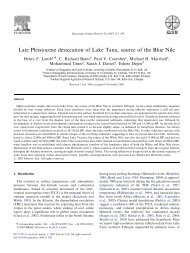


![[pdf] the council - Aberystwyth University](https://img.yumpu.com/8200062/1/184x260/pdf-the-council-aberystwyth-university.jpg?quality=85)